Lightwave Terahertz Quantum Manipulation of Non-equilibrium Superconductor Phases and their Collective Modes

Abstract

We present a gauge-invariant density matrix description of non-equilibrium superconductor (SC) states with spatial and temporal correlations driven by intense terahertz (THz) lightwaves. We derive superconductor Bloch–Maxwell equations of motion that extend Anderson pseudo-spin models to include the Cooper pair center-of-mass motion and electromagnetic propagation effects. We thus describe quantum control of dynamical phases, collective modes, quasi-particle coherence, and high nonlinearities during cycles of carrier wave oscillations, which relate to our recent experiments. Coherent photogeneration of a nonlinear supercurrent with dc component via condensate acceleration by an effective lightwave field dynamically breaks the equilibrium inversion symmetry. Experimental signatures include high harmonic light emission at equilibrium-symmetry-forbidden frequencies, Rabi–Higgs collective modes and quasi-particle coherence, and non-equilibrium moving condensate states tuned by few-cycle THz fields. We use such lightwaves as an oscillating accelerating force that drives strong nonlinearities and anisotropic quasi-particle populations to control and amplify different classes of collective modes, e.g., damped oscillations, persistent oscillations, and overdamped dynamics via Rabi flopping. Recent phase-coherent nonlinear spectroscopy experiments can be modeled by solving the full nonlinear quantum dynamics including self-consistent light–matter coupling.

I Introduction

Recent works have shown that ultrafast phase-coherent THz nonlinear spectroscopy Yang et al. (2019a); Vaswani et al. (2020a); Luo et al. (2017); Chu et al. (2020); Vaswani et al. (2020b) is a powerful tool for sensing and controlling non-equilibrium phases Mitrano et al. (2016); Fausti et al. (2011); Morrison et al. (2014); Porer et al. (2014); Li et al. (2013); Lingos et al. (2017); Shahbazyan et al. (2000a, b); Perakis et al. (1996); Shahbazyan et al. (2000c); Yang et al. (2018a, b) and collective modes Pekker and Varma (2015); Shimano and Tsuji (2020); Giorgianni et al. (2019); Krull et al. (2016); Kumar and Kemper (2019) of quantum materials. For example, the non-equilibrium dynamics of quasi-particles (QPs) in SCs has been characterized and controlled by THz pulses Matsunaga et al. (2013); Yang et al. (2019b). THz quantum quench of the SC order parameter by a single-cycle pulse yields access to a long-lived (10’s of ns) gapless quantum fluid phase of QPs hidden by superconductivity Yang et al. (2018b). By tuning multi-cycle THz pulses, the above QP state changes into non-equilibrium gapless SC, i. e., a moving condensate with gapless excitation spectrum, nearly unchanged macroscopic coherence, and infinite conductivity Yang et al. (2019a); Vaswani et al. (2020a). In all above cases, the dynamics over 100’s of ps is controlled by lightwave few-cycle fields that last for only few ps. Unlike photoexcitation at optical frequencies, THz lightwave electric fields acts as oscillating forces Langer et al. (2016); Hohenleutner et al. (2015); Reimann et al. (2018); Schubert et al. (2014) that accelerate the condensate and, in this way, control its excitation spectrum and order parameter as discussed here.

At the same time, intense efforts have focused on how to use ultrafast THz spectroscopy to detect the collective modes Anderson (1958); Nambu (1960); Bardasis and Schrieffer (1961); Pekker and Varma (2015); Littlewood and Varma (1981, 1982); Varma (2002); Sherman et al. (2015) that characterize quantum phases and symmetry breaking in superconductors Shimano and Tsuji (2020); Matsunaga et al. (2014). In BCS superconductors, the electronic collective modes cannot be probed straightforwardly with linear spectroscopy, as they require finite condensate momentum in order to couple to electromagnetic fields Podolsky et al. (2011); Pekker and Varma (2015). If charge-density order coexists with SC, the amplitude Higgs mode becomes observable with Raman spectroscopy Sooryakumar and Klein (1980); Littlewood and Varma (1981, 1982). Alternatively, with dc supercurrent injection, the Higgs mode can be detected with linear spectroscopy Nakamura et al. (2019); Moor et al. (2017). Identifying amplitude modes in the nonlinear response is possible via third harmonic generation in ultrafast THz spectroscopy, but this is challenging because charge-density fluctuations dominate over the Higgs mode within BCS theory in a clean system Matsunaga et al. (2014); Murotani et al. (2017); Udina et al. (2019). Nevertheless, recent studies argued that Higgs modes can still be observed if electron–phonon coupling or impurities are considered Cea et al. (2018); Murotani and Shimano (2019). Detection of purely electronic amplitude and phase collective modes and dynamical phases in clean superconductors remains an open challenge.

THz ultrafast spectroscopy experiments have been mainly interpreted so far in terms of Anderson pseudo-spin precessions based on Liouville/Bloch equations and nonlinear response functions Papenkort et al. (2007); Podolsky et al. (2011); Pekker and Varma (2015); Murotani et al. (2017); Chou et al. (2017); Udina et al. (2019). However, THz lightwave acceleration  Langer et al. (2016); Hohenleutner et al. (2015); Reimann et al. (2018); Schubert et al. (2014) of the condensate during cycles of carrier wave oscillations and electromagnetic propagation effects have been mostly neglected. Recent experimental observations of high harmonic generation (HHG) at equilibrium-symmetry forbidden frequencies together with long-lived gapless quantum states Yang et al. (2019a); Vaswani et al. (2020a); Yang et al. (2018b) confirmed the importance of Cooper pair center-of-mass momentum. However, such quantum transport effects during THz sub-cycle timescales Yang et al. (2019a); Vaswani et al. (2020a); Langer et al. (2016); Hohenleutner et al. (2015); Reimann et al. (2018); Schubert et al. (2014) require an extension of Anderson pseudo-spin precession models Papenkort et al. (2007); Murotani et al. (2017); Chou et al. (2017); Yu and Wu (2017); Yang and Wu (2019).

In this paper, we discuss a model for analyzing THz phase-coherent nonlinear spectroscopy experiments in quantum materials. This model is based on THz dynamical symmetry breaking during cycles of lightwave oscillations via lightwave condensate acceleration and electromagnetic propagation effects, as well as high Anderson pseudo-spin nonlinearities. For this, we derive a gauge-invariant, non-adiabatic density matrix theory for treating both temporal and spatial fluctuations in combination with Maxwell’s equations. Our theory extends previous studies of quantum transport Stephen (1965); Yu and Wu (2017); Haug and Jauho (2008) and HHG Murotani et al. (2017); Cea et al. (2018) by including the nonlinear dynamics due to self-consistent light–matter electromagnetic coupling. We use this theory to interpret recent experiments Yang et al. (2019a); Vaswani et al. (2020a); Yang et al. (2018b) in terms of THz dynamical symmetry-breaking via nonlinear supercurrent coherent photogeneration. We first present the full nonlinear quantum kinetic theory, which treats spatial and temporal fluctuations, finite Cooper pair center-of-mass condensate momentum $\mathbf{p}_{\mathrm{S}}(t)$, and SC phase dynamics while observing gauge invariance. We then apply a spatial gradient expansion of the full equations that allows the separation of the condensate center-of-mass and Cooper pair relative motions analogous to the theory of ultrafast nonlinear quantum transport in semiconductors Haug and Jauho (2008). We illustrate how a dc nonlinear photocurrent component can be controlled by the cycles of oscillation and the fluence of the pump pulse, as well as by the thickness of a SC film. We also compare the manifestations of charge-density fluctuations and collective modes in the highly nonlinear regime for a one-band BCS model. As a new application of gauge invariant non-perturbative treatment of coupled pseudo-spin precession, lightwave condensate acceleration, and electrodynamics, we demonstrate selective driving and control, by tuning few-cycle THz transient fields, of different classes of collective modes of the SC order parameter, including damped oscillations, persistent (undamped) oscillations, overdamped dynamics, amplified Higgs modes, etc. For example, we demonstrate lightwave coherent control of all three dynamical phases predicted theoretically by “sudden quench” of the SC order parameter Yuzbashyan et al. (2006). We also show that Rabi–Higgs collective modes can be driven by Rabi flopping, which modifies the nonlinear light emission spectrum. The strength of such Rabi–Higgs oscillations is enhanced by the interference between forward-moving and reflected lightwaves inside a nonlinear SC thin film. Explicit calculations of multi-dimensional THz coherent nonlinear spectra will be presented elsewhere. Here we make the point that the nonlinear interplay of Anderson pseudospin precession, Cooper pair quantum transport due to condensate lightwave acceleration, and electromagnetic field propagation effects must be treated self-consistently in the time domain in order to interpret phase-coherent THz nonlinear spectroscopy experiments with well-characterized, phase-coherent, intense THz pulses  Yang et al. (2019a); Vaswani et al. (2020a); Yang et al. (2018b); Langer et al. (2016); Hohenleutner et al. (2015); Reimann et al. (2018); Schubert et al. (2014).

Figure 1 illustrates one of the points made by this paper: Nonlinear photoexcitation of the SC system together with lightwave propagation inside a superconductor thin film results in THz dynamical breaking of the equilibrium inversion symmetry, by photoinducing a dc supercurrent component through nonlinear processes. Of course, the electric field from any physical source does not contain any zero-frequency dc component Kozlov et al. (2011), as a consequence of Maxwell’s equations: $\int_{-\infty}^{\infty}\mathrm{d}t\,E_{\mathrm{THz}}(t)=0$. However, reflected and transmitted electric fields can show a temporal asymmetry and static component after interacting with a nonlinear medium Kozlov et al. (2011). Here, we describe such a process in superconductors and discuss its interplay with pseudo-spin nonlinearities and lightwave sub-cycle condensate acceleration. Our calculations demonstrate nonlinear coherent photogeneration of a dynamical broken-symmetry dc supercurrent, which occurs via the following two steps: (1) THz excitation of the SC film with pump electric field $E_{\mathrm{THz}}(t)$ (red line, Fig. 1(a)) induces a nonlinear ac photocurrent $J_{\mathrm{NL}}(t)$ (yellow line, Fig. 1(b)). (2) Analogous to four-wave mixing, this photocurrent interferes with both forward- and reflected-propagating THz lightwaves inside the SC, which results in coherent photogeneration of a $\omega=0$ component via a third-order nonlinear process. The latter dc component leads to generation of temporally asymmetric reflected ($E_{\mathrm{ref}}(t)$, red line Fig. 1(b)) and transmitted ($E_{\mathrm{trans}}(t)$) electric field pulses with $\int_{-\infty}^{\infty}\mathrm{d}t\,E_{\mathrm{ref},\mathrm{trans}}(t)\neq 0$. Such effective fields in turn drive a dynamically induced condensate flow via lightwave acceleration, which breaks the equilibrium inversion symmetry of the SC system. This THz dynamical symmetry breaking was observed experimentally Yang et al. (2019a); Vaswani et al. (2020a) via high harmonic emission at equilibrium-symmetry forbidden frequencies, particularly at the second harmonic of the THz lightwave driving frequency (red line, Fig. 1(c)). Condensate lightwave acceleration also drives gapless SC non-equilibrium states and collective modes that last longer than the THz pulse, which can be controlled during cycles of carrier wave oscillations.

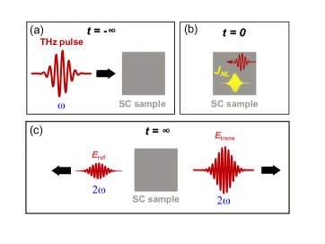
Figure 1: (Color online) Schematic representation of dc supercurrent coherent nonlinear photogeneration leading to equilibrium-symmetry-forbidden second harmonic emission, non-equilibrium gapless SC, and Higgs collective modes via THz dynamical symmetry breaking .

This paper is organized as follows: In Sec. II we present the details of our gauge-invariant density-matrix quantum kinetic theory and the resulting gauge-invariant SC Bloch equations. The self-consistent coupling of the THz-driven SC nonlinearities to the propagating lightwave fields is discussed in Sec. III. In Sec. IV we apply our theory to demonstrate coherent nonlinear photogeneration of a supercurrent with $\omega=0$ component, which controls moving condensate non-equilibrium states with highly nonlinear responses. The experimental detection of such dynamical broken-symmetry supercurrent photogeneration via high-harmonic generation is demonstrated in Sec. V. The selective excitation and sensing of different classes of collective modes of the SC order parameter, coherently controlled by intense THz multi-cycle lightwaves, is presented in Sec. VI. We end with conclusions.

II Gauge-invariant non-adiabatic theory of non-equilibrium superconductivity

In this section, we derive the gauge-invariant density matrix theory that describes the non-equilibrium SC states driven by lightwaves. Here we consider the spatially-dependent Boguliobov–de Gennes Hamiltonian for $s$-wave superconductors Stephen (1965):

$$H=\sum_{\alpha}\int\mathrm{d}^{3}\mathbf{x}\,\psi_{\alpha}^{\dagger}(\mathbf{x})\left[\xi(\mathbf{p}+e\mathbf{A}(\mathbf{x},t))-\mu-e\phi(\mathbf{x},t)\right.$$

$$\left.\qquad\qquad\qquad\qquad\quad+\mu_{\mathrm{H}}(\mathbf{x})+\mu^{\alpha}_{\mathrm{F}}(\mathbf{x})\right]\psi_{\alpha}(\mathbf{x})$$

$$\quad-\int\mathrm{d}^{3}\mathbf{x}\left[\Delta(\mathbf{x})\psi^{\dagger}_{\uparrow}(\mathbf{x})\psi^{\dagger}_{\downarrow}(\mathbf{x})+\mathrm{h.c.}\right]\,,$$ (1)

where the Fermionic field operators $\psi_{\sigma}^{\dagger}(\mathbf{x})$ and $\psi_{\sigma}(\mathbf{x})$ create and annihilate an electron with spin index $\sigma$ and the electromagnetic field is described by the vector potential $\mathbf{A}(\mathbf{x},t)$ and the scalar potential $\phi(\mathbf{x},t)$. $\xi(\mathbf{p}+e\mathbf{A}(\mathbf{x},t))$ is the band dispersion, with momentum operator $\mathbf{p}=-\mathrm{i}\nabla_{\mathbf{x}}$ and electron charge $-e$ ($\hbar$=1). $\mu$ is the chemical potential. The SC order parameter is defined as

$$\Delta(\mathbf{x})=-2\,g\langle\psi_{\downarrow}(\mathbf{x})\psi_{\uparrow}(\mathbf{x})\rangle=|\Delta(\mathbf{x})|\mathrm{e}^{\mathrm{i}\theta(\mathbf{x})}\,,$$ (2)

while

$$\mu_{\mathrm{H}}(\mathbf{x})=2\sum_{\sigma}\int\mathrm{d}^{3}\mathbf{x}^{\prime}\,V(\mathbf{x}-\mathbf{x}^{\prime})n_{\sigma}(\mathbf{x}^{\prime})$$ (3)

is the Hartree energy and

$$\mu^{\alpha}_{\mathrm{F}}(\mathbf{x})=-g\,n_{\alpha}(\mathbf{x})$$ (4)

is the Fock energy, where

$$n_{\sigma}(\mathbf{x})=\langle\psi^{\dagger}_{\sigma}(\mathbf{x})\psi_{\sigma}(\mathbf{x})\rangle$$ (5)

describes the spin-dependent electron populations. Here, $V(\mathbf{x})$ denotes the Coulomb potential, whose Fourier transformation is given by $V_{\mathbf{q}}=e^{2}/(\varepsilon_{0}q^{2})$, and $g$ describes the effective electron–electron pairing interaction in the BCS theory. The Hartree term moves the in-gap Nambu–Goldstone mode up to the plasma frequency due to the long-range Coulomb interaction according to the Anderson–Higgs mechanism Anderson (1958). The Fock energy $\mu^{\alpha}_{\mathrm{F}}(\mathbf{x})$ yields charge conservation of the SC system.

II.1 Gauge-invariant density matrix equations of motion

Gauge invariance of Hamiltonian (II) under the general gauge transformation Nambu (1960)

$$\Psi(\mathbf{x})\,\rightarrow\,\mathrm{e}^{\mathrm{i}\tau_{3}\Lambda(\mathbf{x})/2}\Psi(\mathbf{x})\,,$$ (6)

with the field operator in Nambu space $\Psi(\mathbf{x})=(\psi_{\uparrow}(\mathbf{x}),\psi_{\downarrow}^{\dagger}(\mathbf{x}))^{T}$ and the Pauli spin matrix $\tau_{3}=\begin{pmatrix}1&0\\ 0&-1\end{pmatrix}$, is satisfied when vector potential, scalar potential and SC phase transform as

$$\mathbf{A}(\mathbf{x})\,\rightarrow\,\mathbf{A}(\mathbf{x})+\frac{c}{2e}\nabla\Lambda(\mathbf{x})\,,$$

$$\phi(\mathbf{x})\,\rightarrow\,\phi(\mathbf{x})-\frac{1}{2e}\frac{\partial}{\partial t}\Lambda(\mathbf{x})\,,$$

$$\zeta(\mathbf{x})\,\rightarrow\,\zeta(\mathbf{x})+\Lambda(\mathbf{x})\,.$$ (7)

The density matrix $\rho(\mathbf{x},\mathbf{x}^{\prime})=\langle\Psi(\mathbf{x})^{\dagger}\Psi(\mathbf{x}^{\prime})\rangle$, however, depends on the specific choice of gauge. To define a gauge invariant density matrix, we introduce center-of-mass and relative coordinates $\mathbf{R}=(\mathbf{x}+\mathbf{x}^{\prime})/2$ and $\mathbf{r}=\mathbf{x}-\mathbf{x}^{\prime}$ and introduce a new density matrix Stephen (1965); Yu and Wu (2017); Haug and Jauho (2008)

$$\tilde{\rho}(\mathbf{r},\mathbf{R})= \mathrm{exp}\left[-\mathrm{i}e\int_{0}^{\frac{1}{2}}\mathrm{d}\lambda\,\mathbf{A}(\mathbf{R}+\lambda\,\mathbf{r},t)\cdot\mathbf{r}\,\tau_{3}\right]\,\rho(\mathbf{r},\mathbf{R})$$

$$\times\mathrm{exp}\left[-\mathrm{i}e\int^{0}_{-\frac{1}{2}}\mathrm{d}\lambda\,\mathbf{A}(\mathbf{R}+\lambda\,\mathbf{r},t)\cdot\mathbf{r}\,\tau_{3}\right]\,,$$ (8)

where $\rho(\mathbf{r},\mathbf{R})=\langle\Psi^{\dagger}(\mathbf{R}+\frac{\mathbf{r}}{2})\Psi(\mathbf{R}-\frac{\mathbf{r}}{2}))\rangle$ is the Wigner function. By applying the gauge transformation (6), $\tilde{\rho}(\mathbf{r},\mathbf{R})$ transforms as Yu and Wu (2017)

$$\tilde{\rho}(\mathbf{r},\mathbf{R})\,\rightarrow\,\mathrm{exp}\left[\mathrm{i}\tau_{3}\Lambda(\mathbf{R})/2\right]\tilde{\rho}(\mathbf{r},\mathbf{R})\mathrm{exp}\left[-\mathrm{i}\tau_{3}\Lambda(\mathbf{R})/2\right]\,.$$ (9)

Unlike for the transformed phase of $\rho(\mathbf{r},\mathbf{R})$, which is generally a function of both coordinates $\mathbf{R}$ and $\mathbf{r}$, the phase $\Lambda({\bf R})$ in Eq. (9) depends only on the center-of-mass coordinate. This allows for a gauge-invariant density matrix description of non-equilibrium SC dynamics.

The time evolution of the density matrix (II.1) is obtained by using the Heisenberg equation of motion

$$\mathrm{i}\frac{\partial}{\partial t}\tilde{\rho}=\langle\left[\tilde{\rho},H\right]\rangle\,.$$ (10)

We apply the Fourier transformation with respect to the relative coordinate $\mathbf{r}$,

$$\tilde{\rho}(\mathbf{k},\mathbf{R})=\int\mathrm{d}^{3}\mathbf{r}\,\tilde{\rho}(\mathbf{r},\mathbf{R})\,\mathrm{e}^{-\mathrm{i}\mathbf{k}\cdot\mathbf{r}}\,.$$ (11)

The equation of motion for $\tilde{\rho}(\mathbf{k},\mathbf{R})$ has contributions of the form $\Delta(\mathbf{R}+\frac{\mathrm{i}}{2}\nabla_{\mathbf{k}})\tilde{\rho}(\mathbf{k},\mathbf{R})$, which are evaluated by applying the gradient expansion

$$\Delta(\mathbf{R}+\frac{\mathrm{i}}{2}\nabla_{\mathbf{k}})=\sum_{n=0}^{\infty}\left(\frac{\mathrm{i}}{2}\right)^{n}\frac{(\nabla_{\mathbf{R}}\cdot\nabla_{\mathbf{k}})^{n}}{n!}\Delta(\mathbf{R})\,.$$ (12)

Similar to Ginzburg–Landau theory, this expansion in powers of $\nabla_{\mathbf{R}}\cdot\nabla_{\mathbf{k}}$ can be truncated when the characteristic length for spatial variation of the SC condensate (center of mass) exceeds the coherence length of the Cooper pair (relative motion). To simplify the equations of motion, we also apply the gauge transformation

$$\tilde{\rho}(\mathbf{k},\mathbf{R})=\mathrm{e}^{-\mathrm{i}\tau_{3}\theta(\mathbf{R})/2}\tilde{\rho}(\mathbf{k},\mathbf{R})\mathrm{e}^{\mathrm{i}\tau_{3}\theta(\mathbf{R})/2}\,,$$ (13)

which eliminates the phase of the SC order parameter in the equations of motion. After applying the above gradient expansion and the unitary transformation (13), we obtain the following exact gauge-invariant spatially-dependent SC Bloch equations:

$$\mathrm{i}\frac{\partial}{\partial t}\tilde{\rho}_{1,1}(\mathbf{k},\mathbf{R}) =\left[\xi\left(-\mathbf{k}-\frac{\mathrm{i}}{2}\nabla_{\mathbf{R}}+\mathrm{i}\frac{e}{2}\sum_{n=0}^{\infty}\left(-\frac{1}{4}\right)^{n}\frac{(\nabla_{\mathbf{k}}\cdot\nabla_{\mathbf{R}})^{2n}}{(2n+1)!}\nabla_{\mathbf{k}}\times\mathbf{B}(\mathbf{R})\right.\right.$$

$$\left.\left.\qquad\quad\;-e\sum_{n=1}^{\infty}2n\left(-\frac{1}{4}\right)^{n}\frac{(\nabla_{\mathbf{k}}\cdot\nabla_{\mathbf{R}})^{2n-1}}{(2n+1)!}\nabla_{\mathbf{k}}\times\mathbf{B}(\mathbf{R})\right)\right.$$

$$\quad\;\;\left.-\xi\left(-\mathbf{k}+\frac{\mathrm{i}}{2}\nabla_{\mathbf{R}}-\mathrm{i}\frac{e}{2}\sum_{n=0}^{\infty}\left(-\frac{1}{4}\right)^{n}\frac{(\nabla_{\mathbf{k}}\cdot\nabla_{\mathbf{R}})^{2n}}{(2n+1)!}\nabla_{\mathbf{k}}\times\mathbf{B}(\mathbf{R})\right.\right.$$

$$\left.\left.\qquad\quad\;-e\sum_{n=1}^{\infty}2n\left(-\frac{1}{4}\right)^{n}\frac{(\nabla_{\mathbf{k}}\cdot\nabla_{\mathbf{R}})^{2n-1}}{(2n+1)!}\nabla_{\mathbf{k}}\times\mathbf{B}(\mathbf{R})\right)\right.$$

$$\quad\;\;\left.-2\sum_{n=0}^{\infty}\frac{\left(\frac{\mathrm{i}}{2}\right)^{2n+1}(\nabla_{\mathbf{k}}\cdot\nabla_{\mathbf{R}})^{2n+1}}{(2n+1)!}\left(\mu_{\mathrm{H}}(\mathbf{R})+\mu_{\mathrm{F}}^{\uparrow}(\mathbf{R})\right)\right.$$

$$\quad\;\;\left.-\mathrm{i}e\sum_{n=0}^{\infty}\frac{(\nabla_{\mathbf{k}}\cdot\nabla_{\mathbf{R}})^{2n}}{(2n+1)!}\left(-\frac{1}{4}\right)^{n}\,\mathbf{E}(\mathbf{R})\cdot\nabla_{\mathbf{k}}\right]\tilde{\rho}_{1,1}(\mathbf{k},\mathbf{R})$$

$$+\mathrm{exp}\left[\frac{\mathrm{i}}{2}\nabla_{\mathbf{R}}\cdot\nabla_{\mathbf{k}}\right]|\Delta(\mathbf{R})|\;\mathrm{exp}\left[-\frac{1}{2}\sum_{n=0}^{\infty}\frac{(\nabla_{\mathbf{k}}\cdot\nabla_{\mathbf{R}})^{n}}{(n+1)!}\left(\frac{\mathrm{i}}{2}\right)^{n}\,\mathbf{p}_{\mathrm{S}}(\mathbf{R})\cdot\nabla_{\mathbf{k}}\right]\tilde{\rho}_{2,1}(\mathbf{k},\mathbf{R})$$

$$-\mathrm{exp}\left[-\frac{\mathrm{i}}{2}\nabla_{\mathbf{R}}\cdot\nabla_{\mathbf{k}}\right]|\Delta(\mathbf{R})|\;\mathrm{exp}\left[-\frac{1}{2}\sum_{n=0}^{\infty}\frac{(\nabla_{\mathbf{k}}\cdot\nabla_{\mathbf{R}})^{n}}{(n+1)!}\left(-\frac{\mathrm{i}}{2}\right)^{n}\,\mathbf{p}_{\mathrm{S}}(\mathbf{R})\cdot\nabla_{\mathbf{k}}\right]\tilde{\rho}_{1,2}(\mathbf{k},\mathbf{R})\,,$$ (14)

$$\mathrm{i}\frac{\partial}{\partial t}\tilde{\rho}_{2,2}(\mathbf{k},\mathbf{R}) =\left[\xi\left(\mathbf{k}-\frac{\mathrm{i}}{2}\nabla_{\mathbf{R}}-\mathrm{i}\frac{e}{2}\sum_{n=0}^{\infty}\left(-\frac{1}{4}\right)^{n}\frac{(\nabla_{\mathbf{k}}\cdot\nabla_{\mathbf{R}})^{2n}}{(2n+1)!}\nabla_{\mathbf{k}}\times\mathbf{B}(\mathbf{R})\right.\right.$$

$$\left.\left.\qquad\quad\;+e\sum_{n=1}^{\infty}2n\left(-\frac{1}{4}\right)^{n}\frac{(\nabla_{\mathbf{k}}\cdot\nabla_{\mathbf{R}})^{2n-1}}{(2n+1)!}\nabla_{\mathbf{k}}\times\mathbf{B}(\mathbf{R})\right)\right.$$

$$\quad\;\;\left.-\xi\left(\mathbf{k}+\frac{\mathrm{i}}{2}\nabla_{\mathbf{R}}+\mathrm{i}\frac{e}{2}\sum_{n=0}^{\infty}\left(-\frac{1}{4}\right)^{n}\frac{(\nabla_{\mathbf{k}}\cdot\nabla_{\mathbf{R}})^{2n}}{(2n+1)!}\nabla_{\mathbf{k}}\times\mathbf{B}(\mathbf{R})\right.\right.$$

$$\left.\left.\qquad\quad\;+e\sum_{n=1}^{\infty}2n\left(-\frac{1}{4}\right)^{n}\frac{(\nabla_{\mathbf{k}}\cdot\nabla_{\mathbf{R}})^{2n-1}}{(2n+1)!}\nabla_{\mathbf{k}}\times\mathbf{B}(\mathbf{R})\right)\right.$$

$$\quad\;\;\left.+2\sum_{n=0}^{\infty}\frac{\left(\frac{\mathrm{i}}{2}\right)^{2n+1}(\nabla_{\mathbf{k}}\cdot\nabla_{\mathbf{R}})^{2n+1}}{(2n+1)!}\left(\mu_{\mathrm{H}}(\mathbf{R})+\mu_{\mathrm{F}}^{\downarrow}(\mathbf{R})\right)\right.$$

$$\quad\;\;\left.+\mathrm{i}e\sum_{n=0}^{\infty}\frac{(\nabla_{\mathbf{k}}\cdot\nabla_{\mathbf{R}})^{2n}}{(2n+1)!}\left(-\frac{1}{4}\right)^{n}\,\mathbf{E}(\mathbf{R})\cdot\nabla_{\mathbf{k}}\right]\tilde{\rho}_{2,2}(\mathbf{k},\mathbf{R})$$

$$-\mathrm{exp}\left[-\frac{\mathrm{i}}{2}\nabla_{\mathbf{R}}\cdot\nabla_{\mathbf{k}}\right]|\Delta(\mathbf{R})|\;\mathrm{exp}\left[\frac{1}{2}\sum_{n=0}^{\infty}\frac{(\nabla_{\mathbf{k}}\cdot\nabla_{\mathbf{R}})^{n}}{(n+1)!}\left(-\frac{\mathrm{i}}{2}\right)^{n}\,\mathbf{p}_{\mathrm{S}}(\mathbf{R})\cdot\nabla_{\mathbf{k}}\right]\tilde{\rho}_{2,1}(\mathbf{k},\mathbf{R})$$

$$+\mathrm{exp}\left[\frac{\mathrm{i}}{2}\nabla_{\mathbf{R}}\cdot\nabla_{\mathbf{k}}\right]|\Delta(\mathbf{R})|\;\mathrm{exp}\left[\frac{1}{2}\sum_{n=0}^{\infty}\frac{(\nabla_{\mathbf{k}}\cdot\nabla_{\mathbf{R}})^{n}}{(n+1)!}\left(\frac{\mathrm{i}}{2}\right)^{n}\,\mathbf{p}_{\mathrm{S}}(\mathbf{R})\cdot\nabla_{\mathbf{k}}\right]\tilde{\rho}_{1,2}(\mathbf{k},\mathbf{R})\,,$$ (15)

$$\mathrm{i}\frac{\partial}{\partial t}\tilde{\rho}_{1,2}(\mathbf{k},\mathbf{R}) =\left[-\xi\left(-\mathbf{k}+\frac{\mathrm{i}}{2}\nabla_{\mathbf{R}}-e\sum_{n=0}^{\infty}(2n+1)\left(\frac{\mathrm{i}}{2}\right)^{2n+1}\frac{(\nabla_{\mathbf{k}}\cdot\nabla_{\mathbf{R}})^{2n}}{(2n+2)!}\nabla_{\mathbf{k}}\times\mathbf{B}(\mathbf{R})\right.\right.$$

$$\qquad\qquad\left.\left.-\mathrm{i}\frac{e}{2}\sum_{n=0}^{\infty}\left(\frac{\mathrm{i}}{2}\right)^{2n+1}\frac{(\nabla_{\mathbf{k}}\cdot\nabla_{\mathbf{R}})^{2n+1}}{(2n+2)!}\nabla_{\mathbf{k}}\times\mathbf{B}(\mathbf{R})-\mathbf{p}_{\mathrm{S}}^{\nu_{0}}(\mathbf{R})/2\right)\right.$$

$$\quad\;\;\left.-\xi\left(\mathbf{k}+\frac{\mathrm{i}}{2}\nabla_{\mathbf{R}}+e\sum_{n=0}^{\infty}(2n+1)\left(\frac{\mathrm{i}}{2}\right)^{2n+1}\frac{(\nabla_{\mathbf{k}}\cdot\nabla_{\mathbf{R}})^{2n}}{(2n+2)!}\nabla_{\mathbf{k}}\times\mathbf{B}(\mathbf{R})\right.\right.$$

$$\qquad\qquad\left.\left.+\mathrm{i}\frac{e}{2}\sum_{n=0}^{\infty}\left(\frac{\mathrm{i}}{2}\right)^{2n+1}\frac{(\nabla_{\mathbf{k}}\cdot\nabla_{\mathbf{R}})^{2n+1}}{(2n+2)!}\nabla_{\mathbf{k}}\times\mathbf{B}(\mathbf{R})-\mathbf{p}_{\mathrm{S}}^{\nu_{0}}(\mathbf{R})/2\right)-2\mu_{\mathrm{eff}}(\mathbf{R})\right.$$

$$\quad\;\;\left.-2\sum_{n=0}^{\infty}\frac{\left(\frac{\mathrm{i}}{2}\right)^{2n}(\nabla_{\mathbf{k}}\cdot\nabla_{\mathbf{R}})^{2n}}{(2n)!}\mu_{\mathrm{H}}(\mathbf{R})-\sum_{n=0}^{\infty}\frac{\left(-\frac{\mathrm{i}}{2}\right)^{n}(\nabla_{\mathbf{k}}\cdot\nabla_{\mathbf{R}})^{n}}{n!}\left(\mu_{\mathrm{F}}^{\downarrow}(\mathbf{R})+(-1)^{n}\mu_{\mathrm{F}}^{\uparrow}(\mathbf{R})\right)\right.$$

$$\quad\;\;\left.-\mathrm{i}\,e\,\sum_{n=0}^{\infty}\frac{(\nabla_{\mathbf{k}}\cdot\nabla_{\mathbf{R}})^{2n+1}}{(2n+2)!}\left(\frac{\mathrm{i}}{2}\right)^{2n+1}\,\mathbf{E}(\mathbf{R})\cdot\nabla_{\mathbf{k}}\right]\tilde{\rho}_{1,2}(\mathbf{k},\mathbf{R})$$

$$+\mathrm{exp}\left[\frac{\mathrm{i}}{2}\nabla_{\mathbf{R}}\cdot\nabla_{\mathbf{k}}\right]|\Delta(\mathbf{R})|\mathrm{exp}\left[-\frac{1}{2}\sum_{n=0}^{\infty}\frac{(\nabla_{\mathbf{k}}\cdot\nabla_{\mathbf{R}})^{n}}{(n+1)!}\left(\frac{\mathrm{i}}{2}\right)^{n}\,\mathbf{p}_{\mathrm{S}}(\mathbf{R})\cdot\nabla_{\mathbf{k}}\right]\tilde{\rho}_{2,2}(\mathbf{k},\mathbf{R})$$

$$-\mathrm{exp}\left[-\frac{\mathrm{i}}{2}\nabla_{\mathbf{R}}\cdot\nabla_{\mathbf{k}}\right]|\Delta(\mathbf{R})|\mathrm{exp}\left[\frac{1}{2}\sum_{n=0}^{\infty}\frac{(\nabla_{\mathbf{k}}\cdot\nabla_{\mathbf{R}})^{n}}{(n+1)!}\left(-\frac{\mathrm{i}}{2}\right)^{n}\,\mathbf{p}_{\mathrm{S}}(\mathbf{R})\cdot\nabla_{\mathbf{k}}\right]\tilde{\rho}_{1,1}(\mathbf{k},\mathbf{R})\,.$$ (16)

Here we introduced the gauge-invariant superfluid momentum and effective chemical potential

$$\mathbf{p}_{\mathrm{S}}(\mathbf{R},t)=\nabla_{\mathbf{R}}\theta(\mathbf{R},t)-2e\mathbf{A}(\mathbf{R},t)\,,$$

$$\mu_{\mathrm{eff}}(\mathbf{R},t)=e\,\phi(\mathbf{R},t)+\frac{1}{2}\frac{\partial}{\partial t}\theta(\mathbf{R},t)-\mu\,,$$ (17)

and identified the electric and magnetic fields

$$\mathbf{E}(\mathbf{R})=-\nabla_{\mathbf{R}}\phi(\mathbf{R})-\frac{\partial}{\partial t}\mathbf{A}(\mathbf{R})\,,\quad\mathbf{B}(\mathbf{R})=\nabla_{\mathbf{R}}\times\mathbf{A}(\mathbf{R})\,.$$ (18)

The Higgs collective mode corresponds to amplitude fluctuations of the SC order parameter

$$\Delta(\mathbf{R})=-2g\sum_{\mathbf{k}}\mathrm{exp}\left[e\sum_{n=0}^{\infty}\left(\frac{\mathrm{i}}{2}\right)^{2n+1}\frac{(\nabla_{\mathbf{k}}\cdot\nabla_{\mathbf{R}})^{2n+1}}{(2n+2)!}\mathbf{p}_{\mathrm{S}}(\mathbf{R})\cdot\nabla_{\mathbf{k}}\right]\tilde{\rho}_{2,1}(\mathbf{k},\mathbf{R})\,.$$ (19)

The light-driven dynamics of the phase of the SC order parameter $\Delta(\mathbf{R})$ is determined by the equation of motion

$$\frac{\partial}{\partial t}\theta(\mathbf{R}) =-2\left(e\,\phi(\mathbf{R})-\,\mu-\mu_{\mathrm{H}}(\mathbf{R})-\frac{1}{2}(\mu_{\mathrm{F}}^{\uparrow}(\mathbf{R})+\mu_{\mathrm{F}}^{\downarrow}(\mathbf{R}))\right)$$

$$+\frac{g}{|\Delta(\mathbf{R})|}\sum_{\mathbf{k}}\left(\left[\xi(\mathbf{k}+\frac{\mathrm{i}}{2}\nabla_{\mathbf{R}}-\mathbf{p}_{\mathrm{S}}(\mathbf{R})/2)+\xi(\mathbf{k}-\frac{\mathrm{i}}{2}\nabla_{\mathbf{R}}+\mathbf{p}_{\mathrm{S}}(\mathbf{R})/2)\right]\tilde{\rho}_{1,2}(\mathbf{k},\mathbf{R})\right.$$

$$\left.\qquad\qquad\qquad\qquad\quad+\left[\xi(\mathbf{k}-\frac{\mathrm{i}}{2}\nabla_{\mathbf{R}}-\mathbf{p}_{\mathrm{S}}(\mathbf{R})/2)+\xi(\mathbf{k}+\frac{\mathrm{i}}{2}\nabla_{\mathbf{R}}+\mathbf{p}_{\mathrm{S}}(\mathbf{R})/2)\right]\tilde{\rho}_{2,1}(\mathbf{k},\mathbf{R})\right)$$

$$+\frac{2g}{|\Delta(\mathbf{R})|}\sum_{\mathbf{k}}|\Delta(\mathbf{R})|\left[\tilde{\rho}_{1,1}(\mathbf{k},\mathbf{R})-\tilde{\rho}_{2,2}(\mathbf{k},\mathbf{R})\right]\,.$$ (20)

The lightwave field accelerates the center-of-mass of the Cooper-pairs with gauge-invariant momentum determined by the electric field and by spatial fluctuations:

$$\frac{\partial}{\partial t}\mathbf{p}_{\mathrm{S}}(\mathbf{R},t) =2\nabla_{\mathbf{R}}\mu_{\rm{eff}}({\bf R},t)+2e\,\mathbf{E}(\mathbf{R},t).\,$$ (21)

As seen from Eq. (17), the time-dependent changes in the SC order parameter phase are included in the above equation of motion and determine the condensate center-of-mass momentum $\mathbf{p}_{\mathrm{S}}({\bf R},t)$. The latter develops here as a result of lightwave acceleration of the macroscopic Cooper pair state. This acceleration is strong in the case of intense THz fields available today and therefore we include $\mathbf{p}_{\mathrm{S}}({\bf R},t)$ in the above density matrix equations of motion without perturbative expansions. For example, lightwave acceleration displaces the populations and coherences in momentum space by $\mathbf{p}_{\mathrm{S}}(t)/2$, which unlike in previous works are treated exactly here. In this way, we describe the breaking of the equilibrium inversion symmetry of electron ($\tilde{\rho}_{1,1}(\mathbf{k},\mathbf{R})$) and hole ($\tilde{\rho}_{2,2}(\mathbf{k},\mathbf{R})$) populations, as the condensate momentum vector defines a preferred direction. The lightwave condensate acceleration is described by quantum transport terms of the form $\mathbf{E}(\mathbf{R})\cdot\nabla_{\mathbf{k}}\tilde{\rho}(\mathbf{k},\mathbf{R})$ in the equations of motion (II.1)–(II.1). The latter are absent in the pseudo-spin precession model Chou et al. (2017) and lead to linear couplings of the electric field. Higher orders in the spatial gradient expansion, e. g. the first ($\mathcal{O}(\nabla_{\mathbf{k}}\cdot\nabla_{\mathbf{R}})$) and second order terms ($\mathcal{O}((\nabla_{\mathbf{k}}\cdot\nabla_{\mathbf{R}})^{2})$), contain the kinetic terms in the Ginzburg–Landau equation Yang and Wu (2018). Such spatial contributions can be expanded as in Ginzburg–Landau theory.

The Fock energies in the above gauge-invariant density matrix equations of motion,

$$\mu_{\mathrm{F}}^{\uparrow}(\mathbf{R})=-g\sum_{\mathbf{k}} \mathrm{exp}\left[e\sum_{n=0}^{\infty}\left(\frac{\mathrm{i}}{2}\right)^{2n}\frac{(\nabla_{\mathbf{k}}\cdot\nabla_{\mathbf{R}})^{2n}}{(2n+1)!}\mathbf{p}_{\mathrm{S}}(\mathbf{R})\cdot\nabla_{\mathbf{k}}\right]\tilde{\rho}_{1,1}(\mathbf{k},\mathbf{R})\,,$$

$$\mu_{\mathrm{F}}^{\downarrow}(\mathbf{R})=-g\sum_{\mathbf{k}} \left(1-\mathrm{exp}\left[-e\sum_{n=0}^{\infty}\left(\frac{\mathrm{i}}{2}\right)^{2n}\frac{(\nabla_{\mathbf{k}}\cdot\nabla_{\mathbf{R}})^{2n}}{(2n+1)!}\mathbf{p}_{\mathrm{S}}(\mathbf{R})\cdot\nabla_{\mathbf{k}}\right]\tilde{\rho}_{2,2}(\mathbf{k},\mathbf{R})\right)\,,$$ (22)

ensure charge conservation of the SC system. In particular, the gauge-invariant current,

$$\mathbf{J}(\mathbf{R})=e\sum_{\mathbf{k}}\nabla_{\mathbf{k}}\xi(\mathbf{k})\left[\tilde{\rho}_{1,1}(\mathbf{k},\mathbf{R})+\tilde{\rho}_{2,2}(\mathbf{k},\mathbf{R})\right]\,,$$ (23)

and electron density,

$$n(\mathbf{R})=\sum_{\mathbf{k}}\left[1+\tilde{\rho}_{1,1}(\mathbf{k},\mathbf{R})-\tilde{\rho}_{2,2}(\mathbf{k},\mathbf{R})\right]\,,$$ (24)

explicitly satisfy the continuity equation

$$e\frac{\partial}{\partial t}n(\mathbf{R})+\nabla_{\mathbf{R}}\cdot\mathbf{J}(\mathbf{R})=0\,,$$ (25)

which is a direct consequence of the gauge invariance of the equations of motion (II.1)–(II.1). The SC phase and amplitude dynamics as well as spatial dependence are thus treated consistently.

II.2 Homogeneous SC system

For weak spatial dependence and homogeneous excitation conditions, we neglect all terms of order $\mathcal{O}(\nabla_{\mathbf{k}}\cdot\nabla_{\mathbf{R}})$ and higher in the gradient expansion (12), as well as the $\mathbf{R}$-dependence of $\mathbf{E}$- and $\mathbf{B}$-fields, in the equations of motion (II.1)–(II.1). We then obtain the gauge-invariant homogenous SC Bloch equations valid for any condensate center-of-mass momentum ${\bf p}_{\mathrm{S}}(t)$:

$$\mathrm{i}\frac{\partial}{\partial t}\tilde{\rho}_{1,1}(\mathbf{k})=-\mathrm{i}\,e\,\mathbf{E}(t)\cdot\nabla_{\mathbf{k}}\tilde{\rho}_{1,1}(\mathbf{k})-|\Delta|\left[\tilde{\rho}_{1,2}(\mathbf{k}-\mathbf{p}_{\mathrm{S}}/2)-\tilde{\rho}_{2,1}(\mathbf{k}-\mathbf{p}_{\mathrm{S}}/2)\right]\,,$$

$$\mathrm{i}\frac{\partial}{\partial t}\tilde{\rho}_{2,2}(\mathbf{k})=\mathrm{i}\,e\,\mathbf{E}(t)\cdot\nabla_{\mathbf{k}}\tilde{\rho}_{2,2}(\mathbf{k})+|\Delta|\left[\tilde{\rho}_{1,2}(\mathbf{k}+\mathbf{p}_{\mathrm{S}}/2)-\tilde{\rho}_{2,1}(\mathbf{k}+\mathbf{p}_{\mathrm{S}}/2)\right]\,,$$

$$\mathrm{i}\frac{\partial}{\partial t}\tilde{\rho}_{1,2}(\mathbf{k})=-[\xi(\mathbf{k}-\mathbf{p}_{\mathrm{S}}/2)+\xi(-\mathbf{k}-\mathbf{p}_{\mathrm{S}}/2)+2(\mu_{\mathrm{eff}}+\mu_{\mathrm{F}})]\tilde{\rho}_{1,2}(\mathbf{k})$$

$$\qquad\qquad\quad\;\;+|\Delta|\left[\tilde{\rho}_{2,2}(\mathbf{k}-\mathbf{p}_{\mathrm{S}}/2)-\tilde{\rho}_{1,1}(\mathbf{k}+\mathbf{p}_{\mathrm{S}}/2)\right]\,,$$ (26)

where

$$\mathbf{p}_{\mathrm{S}}=-2\,e\,\mathbf{A}\,,\quad\mu_{\mathrm{eff}}=e\,\phi+\frac{1}{2}\frac{\partial}{\partial t}\theta-\mu\,,$$

$$|\Delta|=-2g\sum_{\mathbf{k}}\tilde{\rho}_{2,1}(\mathbf{k})\,,$$

$$\mu_{\mathrm{F}}\equiv\frac{1}{2}\left(\mu^{\downarrow}_{\mathrm{F}}+\mu^{\uparrow}_{\mathrm{F}}\right)=-g\sum_{\mathbf{k}}\left[1+\tilde{\rho}_{1,1}(\mathbf{k})-\tilde{\rho}_{2,2}(\mathbf{k})\right]\,.$$ (27)

The equations of motion for condensate momentum $\mathbf{p}_{\mathrm{S}}$ and SC order parameter phase $\theta$ simplify to

$$\frac{\partial}{\partial t}\mathbf{p}_{\mathrm{S}}=2e\,\mathbf{E}\,$$ (28)

and

$$\frac{\partial}{\partial t}\theta=-2\left(e\,\phi-\,\mu-\mu_{\mathrm{F}}\right)$$

$$+\frac{g}{|\Delta|}\sum_{\mathbf{k}}\left[\xi(\mathbf{k}-\mathbf{p}_{\mathrm{S}}/2)+\xi(\mathbf{k}+\mathbf{p}_{\mathrm{S}}/2)\right]\left(\tilde{\rho}_{1,2}(\mathbf{k})+\tilde{\rho}_{2,1}(\mathbf{k})\right)$$

$$+\frac{2g}{|\Delta|}\sum_{\mathbf{k}}|\Delta|\left[\tilde{\rho}_{1,1}(\mathbf{k})-\tilde{\rho}_{2,2}(\mathbf{k})\right].$$ (29)

The gauge-invariant Bloch equations Eq. (II.2) reduce to the Anderson pseudo-spin precession model by omitting the transport terms $\propto\mathbf{E}(t)$, the ${\bf p}_{\mathrm{S}}(t)/2$-displacement of populations and coherences, and the SC phase and Fock contributions to the chemical potential.

There are three ways in which the lightwave fields couple to the SC in Eq. (II.2) in the spatially homogeneous limit: (1) First, the familiar minimal coupling, $\xi(\mathbf{k}-\mathbf{p}_{\mathrm{S}}/2)+\xi(-\mathbf{k}-\mathbf{p}_{\mathrm{S}}/2)$, drives even-order nonlinearities of the SC order parameter. This coupling depends on the electron band dispersion non-parabolicity and can be expanded in $\mathcal{O}(p_{s}^{2n})$=$\mathcal{O}(A^{2n})$ even terms  Matsunaga et al. (2014). This coupling does not contribute to the linear response Pekker and Varma (2015) and has been studied before in the context of the Anderson pseudo-spin precession model. (2) Second, the condensate acceleration by the lightwave effective field results in SC order parameter nonlinearities that are of odd order in the electric field. These THz nonlinear quantum transport contributions come from terms of the form $\mathrm{i}\,e\mathbf{E}(t)\cdot\nabla_{\mathbf{k}}\tilde{\rho}(\mathbf{k})$ in Eq. (II.2). (3) Third, for accelerated condensate with finite center-of-mass momentum, the population and coherence displacements in momentum space by $\pm\mathbf{p}_{\mathrm{S}}/2$ are treated non-perturbatively for intense THz fields. In particular, with lightwave acceleration, we thus describe a non-equilibrium moving condensate consisting of Cooper pairs formed by $({\bf k}+\mathbf{p}_{\mathrm{S}}(t)/2,\uparrow)$ and $(-{\bf k}+\mathbf{p}_{\mathrm{S}}(t)/2,\downarrow)$ electrons. A large momentum ${\bf p}_{\mathrm{S}}(t)$ then leads to a lightwave-induced anisotropy in momentum space, which results in new non-perturbative contributions for $\Delta\neq 0$. Note that ${\bf p}_{\mathrm{S}}(t)$ is determined by self-consistent non-perturbative coupling between the propagating electromagnetic fields and the nonlinear supercurrent, discussed next.

III Self-consistent coupling between propagating electromagnetic field and nonlinear supercurrent

To include lightwave propagation effects, we use from Maxwell’s wave equation for the electric field Zhou (1991); Hirsch (2004)

$$\left[\nabla_{\mathbf{r}}^{2}-\frac{n(\mathbf{r})^{2}}{c^{2}}\frac{\partial^{2}}{\partial t^{2}}\right]\mathbf{E}(\mathbf{r},t)=-\mu_{0}\frac{\partial}{\partial t}\mathbf{J}(\mathbf{r},t)\,$$ (30)

for background refractive index $n(\mathbf{r})$. The above equation describes the effective lightwave field that drives the SC condensate, which is modified as compared to the applied laser field due to the coupling with the nonlinear supercurrent Eq. (23). By decomposing the electric field into components parallel and perpendicular ($z$-direction) to the SC film, $\mathbf{E}=\mathbf{E}_{\perp}+\mathbf{E}_{\parallel}$, and applying Fourier transformation with respect to the in-plane coordinates $(x,y)={\bf\rho}$,

$$\mathbf{E}(\rho,z,t)=\frac{1}{S}\sum_{\mathbf{q}_{\parallel}}\mathrm{e}^{\mathrm{i}\mathbf{q}_{\parallel}\cdot\rho}\mathbf{E}(\mathbf{q}_{\parallel},z,t)\,,$$ (31)

we transform the wave equation for the in-plane electric field into

$$\left[\frac{\partial^{2}}{\partial z^{2}}-q_{\parallel}^{2}-\frac{n(z)^{2}}{c^{2}}\frac{\partial^{2}}{\partial t^{2}}\right]\mathbf{E}_{\parallel}(\mathbf{q}_{\parallel},z,t)=-\mu_{0}\frac{\partial}{\partial t}\mathbf{J}_{\parallel}(\mathbf{q}_{\parallel},z,t)\,.$$ (32)

We next assume that the externally applied electric field propagates perpendicular to the film, such that the wave vector parallel to the film vanishes, i. e. $\mathbf{q}_{\parallel}=0$, and there is only $z$-dependence. As a result, lightwave propagation inside the SC film can be described by the one-dimensional wave equation

$$\left[\frac{\partial^{2}}{\partial z^{2}}-\frac{n(z)^{2}}{c^{2}}\frac{\partial^{2}}{\partial t^{2}}\right]\mathbf{E}_{\parallel}(z,t)=-\mu_{0}\frac{\partial}{\partial t}\mathbf{J}_{\parallel}(z,t)\,.$$ (33)

When the wavelength of the applied laser field exceeds the thickness of the SC film, we can approximate the $z$-dependence of the current by $\mathbf{J}_{\parallel}(z,t)=\delta(z)\mathbf{J}_{\parallel}(t)$, such that the wave equation becomes

$$\left[\frac{\partial^{2}}{\partial z^{2}}-\frac{n(z)^{2}}{c^{2}}\frac{\partial^{2}}{\partial t^{2}}\right]\mathbf{E}_{\parallel}(z,t)=-\mu_{0}\frac{\partial}{\partial t}\delta(z)\mathbf{J}_{\parallel}(t)\,.$$ (34)

Assuming that substrate and SC film have comparable background refractive index $n$, Eq. (34) can be solved analytically, yielding the self-consistent electric field Jahnke et al. (1997)

$$\mathbf{E}(z,t)=\mathbf{E}_{0}(z,t)-\mu_{0}\frac{c}{2n}\mathbf{J}_{\parallel}(t-|nz|/c)\,,$$ (35)

where $\mathbf{E}_{0}(z,t)$ denotes the externally applied electric field, incident on the SC film from the left, i. e. $z<0$. The reflected and transmitted electric fields are given by  Jahnke et al. (1997)

$$\mathbf{E}_{\mathrm{ref}}(z,t)=-\mu_{0}\frac{c}{2n}\mathbf{J}_{\parallel}(t-|nz|/c)\,,\qquad z\leq 0\,,$$

$$\mathbf{E}_{\mathrm{trans}}(z,t)=\mathbf{E}_{0}(z,t)-\mu_{0}\frac{c}{2n}\mathbf{J}_{\parallel}(t-|nz|/c)\,,\qquad z\geq 0\,.$$ (36)

The effective field that drives ${\bf p}_{\mathrm{S}}(t)$, Eq. (21), is modified as compared to the incident field by the reflected field determined by the supercurrent. The latter, in turn, depends on the displaced populations and coherences determined by ${\bf p}_{\mathrm{S}}(t)$. The effects of this non-perturbative self-consistent coupling are discussed next.

IV Lightwave propagation effects on the non-equilibrium SC dynamics

In this section, we demonstrate that photo-excited SC nonlinearities, together with lightwave propagation inside a SC thin film system, can lead to coherent photogeneration of a nonlinear supercurrent with a dc component and a gapless moving condensate non-equilibrium state with tunable superfluid density. For our numerical calculations, we use the square lattice nearest-neighbor tight-binding dispersion $\xi(\mathbf{k})=-2\,J[\mathrm{cos}(k_{x}\,a)+\mathrm{cos}(k_{y}\,a)]+\mu$, with hopping parameter $J$, lattice constant $a$, and band-offset $\mu$. We only consider the half-filling limit $(\mu=0)$ where particle-hole symmetry is realized. As initial state, we take the BCS ground state with SC gap $2\Delta=5.1$  meV. To compute the dynamics of the gauge-invariant density matrix (11) without perturbative expansions, we self-consistently solve the SC Bloch equations (II.2) and the equations for the SC gap and the Fock energy (II.2) together with Eq. (35), using a fourth-order Runge–Kutta method. We excite the system with external THz electric field $\mathbf{E}_{\mathrm{THz}}(t)=E_{0}\,\mathbf{e}_{x}\,\mathrm{sin}(\omega_{0}\,t)\,\mathrm{exp}[-t^{2}/(2\,\sigma_{t}^{2})]$, where $E_{0}$ is the field amplitude that defines its strength, $\omega_{0}$ corresponds to the central frequency, and $\sigma_{t}$ determines the duration of the applied $\mathbf{E}$-field. The external pump $\mathbf{E}$-field satisfies the condition $\int_{-\infty}^{\infty}\mathrm{d}t\,\mathbf{E}_{\mathrm{THz}}(t)=0$, i.e. $\mathbf{E}_{\mathrm{THz}}(t)$ does not contain any zero-frequency dc component. This is a condition which every physical source of electromagnetic waves must satisfy according to Maxwell’s equations.

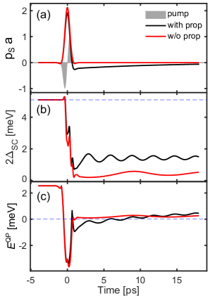
Figure 2: Time evolution of BCS state into a gapless non-equilibrium SC state after strong THz quantum quench. (a) Dynamics of THz-light-induced superfluid momentum $p_{\mathrm{S}}(t)$. We compare the calculations with electromagnetic propagation effects (black line, effective driving field differs from external field) and without (red line, driving field coincides with external field), together with a representative single-cycle 0.5 THz pump electric field (shaded area). The effective driving field, determined self-consistently by Maxwell’s equations and the nonlinear supercurrent, accelerates the condensate, with a center-of-mass momentum that decays slowly in time. (b) The corresponding dynamics of the SC order parameter; horizontal dashed line indicates the equilibrium value of the SC order parameter. The condensate density remains finite after the pulse when electromagnetic propagation effects are included. (c) The corresponding dynamics of the minimum QP excitation energy. A gapless QP anisotropic spectrum with finite order parameter is obtained after the pulse when electromagnetic propagation effects are included.

Figure 2(a) shows the dynamics of the superfluid momentum $\mathbf{p}_{\mathrm{S}}(t)$ driven by a short 0.5 THz pulse (shaded area). We compare our calculations without (red line) and with electromagnetic propagation effects (black line). The latter leads to an effective electric field whose temporal profile differs from the external THz pulse. The SC time evolution is driven by this effective field, which depends self-consistently on the nonlinear photocurrent. Such excitation of the SC system induces a superfluid momentum during the pulse, which persists after the pulse only when the electromagnetic propagation effects are included. The condensate center-of-mass momentum decays in time due to radiative damping, which is a consequence of the self-consistent coupling between the nonlinear photocurrent and the lightwave $\mathbf{E}$-field. The calculated momentum relaxation rate $\Gamma$, derived in Appendix A, depends on the details of the bandstructure and is stronger for superconductors with a large density of states at the Fermi surface Vaswani et al. (2020a).

Due to the condensate motion, ${\bf p}_{\mathrm{S}}\neq 0$, the SC order parameter 2$\Delta$ no longer coincides with the QP excitation gap. The dynamics of $\Delta(t)$ and the QP excitation energy are plotted in Figs. 2(b) and (c). Here the QP excitation energy is defined as the minimum of the QP energy $E^{\mathrm{QP}}_{\mathbf{k}}$ among all $\mathbf{k}$ around the Fermi surface, with $E^{\mathrm{QP}}_{\mathbf{k}}$ given by Eq. (48). The results of our calculations with or without electromagnetic propagation effects both show a quench of the SC order parameter followed by Higgs oscillations. At the same time, the QP excitation spectrum can transiently become gapless during the pulse for sufficiently high fields, i.e. $E^{\mathrm{QP}}\leq 0$ for some $\mathbf{k}$. However, for the calculation where electromagnetic propagation effects are included, we obtain a non-equilibrium state where the QP excitation spectrum is also gapless after the pulse for sufficiently strong fields. Despite this gapless excitation spectrum, the SC order parameter remains finite, which corresponds to a gapless condensate non-equilibrium state consistent with recent experimental observations Yang et al. (2019a). The above controllable gapless non-equilibrium quantum state arises from THz dynamical symmetry breaking in a moving condensate, which is absent for the standard Anderson pseudo-spin model. With lightwave acceleration during cycles of carrier wave oscillations, we can thus non-adiabatically drive a gapless SC quantum phase with finite condensate coherence in a SC thin film. For this quantum state, $\Delta>0$ while $E^{\mathrm{QP}}_{\mathbf{k}}\leq 0$ for several $\mathbf{k}$-points. For the same pump electric field, a quenched SC state with $\Delta>0$ and $E^{\mathrm{QP}}_{\mathbf{k}}>0$ is obtained if the electromagnetic propagation effects are neglected.

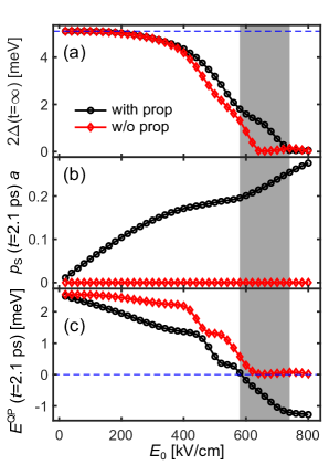
Figure 3: Control of THz-driven non-equilibrium SC state by pump electric field strength. (a) Pump field amplitude dependence of the steady state SC order parameter reached after the pulse. We compare the calculations with electromagnetic propagation effects (black line, effective driving field differs from external pulse) and without (red line, driving field coincides with external THz laser pulse). Shaded area indicates phase (II) with finite condensate density but gapless excitation spectrum. (b), (c) The corresponding $E_{0}$-field dependence of the superfluid momentum and QP excitation energy.

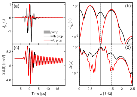
Figure 4: Detection of THz dynamical inversion symmetry breaking by HHG. (a) Dynamics of THz-light-induced nonlinear current $\mathbf{J}_{\mathrm{NL}}(t)$ for a calculation with (black line) and without electromagnetic propagation effects (red line), shown together with a representative 0.5 THz electric pump field used in the calculations (shaded area). (b) The corresponding supercurrent spectra in semi-logarithmic scale. Vertical solid (dashed) lines indicate equilibrium-symmetry allowed (forbidden) harmonics. (c), (d) The corresponding dynamics and spectra of the SC order parameter.

Figure 3 illustrates our conclusion that THz lightwave propagation inside the SC system can selectively drive three different non-equilibrium quantum phases (I)-(III) after the pulse. This result opens up possibilities for coherent control, as the calculated light-tunable transient quantum states define a systematic initial condition for post-quench long-time dynamics that is consistent with recent experiments Yang et al. (2018b); Vaswani et al. (2020a). The $E_{0}$-field dependence of the steady state SC order parameter reached after the pulse (Fig. 3(a)), the laser-induced superfluid momentum (Fig. 3(b)), and the QP excitation energy slightly after the pump pulse (Fig. 3(c)) are shown for a calculation with (black line) and without (red line) propagation effects. Without lightwave propagation inside the SC system, increasing the pump field amplitude $E_{0}$ can only drive a quenched SC state with $\Delta>0$ and $E^{\mathrm{QP}}>0$ (regime I) or a gapless QP state with $\Delta=0$ and $E^{\mathrm{QP}}=0$ (regime III). In this case, $\mathbf{p}_{\mathrm{S}}\neq 0$ only during the electromagnetic pulse. The steady states after the pulse are then similar to the quantum states obtained after “sudden quench” of the order parameter Yuzbashyan et al. (2006); Chou et al. (2017). Compared to that, photo-excited nonlinearities together with lightwave propagation inside the superconductor lead to a finite center-of-mass momentum of the accelerated condensate after the pulse, which can drive a gapless SC state with finite coherence (order parameter) across a wide range of $E_{0}$ (shaded area, regime II). This result is consistent with the experimental observations in Ref. Yang et al. (2019a) and cannot be obtained by using the standard Anderson pseudo-spin Hamiltonian without including the lightwave quantum transport effects. Lightwave sub-cycle acceleration results in an oscillating condensate center-of-mass momentum $\mathbf{p}_{\mathrm{S}}$ that remains finite after the pulse due to THz dynamical symmetry breaking in a thin film geometry. This lightwave acceleration modulates the SC excitation spectrum, which can transiently close and reopen during cycles of carrier wave oscillations. In addition to coherently controlling gapless non-equilibrium SC, the above THz dynamical symmetry breaking and coherent nonlinear supercurrent photogeneration manifest themselves in HHG at equilibrium-symmetry-forbidden frequencies, discussed next.

V Experimental detection of lightwave dynamical symmetry breaking: coherent control of high-harmonics generation

As shown in the previous section, photo-excited SC nonlinearities together with lightwave propagation effects can lead to coherent photogeneration of a nonlinear supercurrent with a $\omega\approx 0$ component. In addition to driving gapless SC states after the pulse, such THz dynamical inversion symmetry breaking allows us to coherently control HHG in the nonlinear response via the momentum and excitations of the moving condensate state during cycles of carrier wave oscillation. For a driving field with $\int_{-\infty}^{\infty}\mathrm{d}t\,\mathbf{E}_{\mathrm{THz}}(t)=0$, the condensate center-of-mass momentum $\mathbf{p}_{\mathrm{S}}(t)$ oscillates symmetrically in time with the pump laser’s frequency $\omega_{\mathrm{0}}$. $\mathcal{O}(\mathbf{p}_{\mathrm{S}}^{2})$ terms in the equations of motion (II.2) then drive a temporal evolution of the density matrix $\tilde{\rho}(\mathbf{k})$ with symmetry-allowed frequency oscillations at $2\omega_{\mathrm{0}}$. The nonlinear contributions to the equations of motion also produce higher even harmonics $4\omega_{\mathrm{0}},\,6\omega_{\mathrm{0}},\dots$ in the density matrix time evolution. As a result, the current $\mathbf{J}$ (order parameter $\Delta$) shows odd (even) harmonics of the pump laser pulse’s frequency. The above situation changes, however, when electromagnetic propagation effects are included to obtain the real driving field. As discussed in the previous sections, the latter can lead to inversion symmetry breaking of the electron and hole distributions in momentum space that persists after the pulse. The spectrum of $\mathbf{p}_{\mathrm{S}}(\omega)$ now shows a small zero-frequency light-induced nonlinear component, in addition to the peak at $\omega_{0}$. Such dc contribution results from the effective electric field that accelerates ${\bf p}_{\mathrm{S}}(t)$, which is modified from the external field by the oscillating nonlinear supercurrent. As a result of THz dynamical symmetry breaking, the Fourier transformation of $\mathbf{J}$ ($\Delta$) will exhibit equilibrium-symmetry forbidden even (odd) harmonics, in addition to the well-known odd (even) harmonics. While the Anderson pseudo-spin model predicts third harmonic generation studied in the past, THz dynamical symmetry breaking during cycles of lightwave oscillations leads to forbidden HHG modes recently observed experimentally Vaswani et al. (2020a).

To test the above perspective, we plot in Fig. 4(a) the dynamics of THz-light-induced nonlinear supercurrent $\mathbf{J}_{\mathrm{NL}}(t)$ for a calculation with (black line) and without (red line) electromagnetic propagation effects. Here, the SC system is excited with a 8 ps THz pulse (shaded area). Since a linear photocurrent only produces a $\omega_{\mathrm{0}}$-frequency contribution, we focus on the nonlinear photocurrent. The latter exhibits third harmonic oscillations, i. e. oscillates with $3\,\omega_{0}$, higher harmonics, and a small dc component $J_{\mathrm{dc}}$ that decays slowly with a rate $\Gamma$ calculated in appendix A. Also, $\mathbf{J}_{\mathrm{NL}}$ shows pronounced amplitude Higgs oscillations due to the photoinduced $J_{\mathrm{dc}}$ that breaks the symmetry. A Fourier transformation of the nonlinear current temporal profile allows us to disentangle the different nonlinear optical processes contributing to $\mathbf{J}_{\mathrm{NL}}(t)$. The calculated emission spectrum, $I(\omega)=|\mathbf{J}_{\mathrm{NL}}(\omega)|^{2}$, at energy $\hbar\omega$ is presented in Fig. 4(b) in semi-logarithmic scale. While the spectrum resulting from the calculation without propagation effects shows only odd harmonics (solid vertical lines), the result of the full calculation yields odd as well as even harmonics (dashed vertical lines). To confirm that the broken inversion symmetry of the non-equilibrium state can be detected by HHG, Figs. 4(c) and (d) present the corresponding dynamics and spectra of the SC order parameter. Without electromagnetic propagation effects, $\Delta(\omega)$ only shows even harmonics, while lightwave propagation inside the SC system leads also to the generation of equilibrium-symmetry-forbidden odd harmonics. The latter demonstrates that THz dynamical inversion symmetry breaking induced by nonlinear supercurrent coherent photogeneration is directly detectable by HHG. Such nonlinear response presents a direct experimental verification of the theoretically predicted effect, confirmed in Ref. Vaswani et al. (2020a), and can be coherently controlled by tuning the applied few-cycle field.

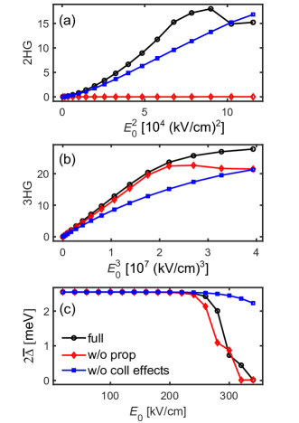
Figure 5: Electric field strength $E_{0}$ dependence of HHG. (a) Second harmonic emission as a function of electric field strength; the full calculation (black line) is compared with a calculation where electromagnetic propagation effects (red line) and light-induced changes in the collective effects (blue line) are switched off. (b), (c) The corresponding $E_{0}$-dependence of third harmonic generation and the average value of the SC order parameter in the steady state after the THz pulse, $\bar{\Delta}$.

We next investigate the electric field strength dependence of HHG and identify the nonlinearities contributing to each different HHG peak by applying a switch-off analysis. Figures 5(a) and (b) show the electric field strength dependence of second (forbidden) harmonic and third harmonic generation, respectively, while the average value of the SC order parameter in the steady state after the THz pulse, $\bar{\Delta}$, is plotted in Fig. 5(c). The full calculation (black line) is compared with a calculation where electromagnetic propagation effects (red line) and light-induced changes in collective effects (blue line) are switched off. The role of light-induced collective effects and corresponding interaction-induced nonlinearities is revealed by replacing $\Delta(t)$ by the equilibrium SC gap $\Delta_{0}$ on the right-hand side of the equation of motions Anderson (1958). In this case, the fluctuations, $\delta\Delta(t)=\Delta(t)-\Delta_{0}$, of the SC order parameter are neglected, so the response is fully determined by charge-density fluctuations. For the full calculation, the emitted intensity of second (third) harmonics grows linearly as a function of $E_{0}^{2}$ ($E_{0}^{3}$) at low pump fields, before saturating at elevated $E_{0}$, where the SC order parameter becomes quenched (Fig. 5(c)). While switching off propagation effects only slightly reduces the third harmonic emission, second harmonic emission is zero in this case, due to persisting inversion symmetry. Compared to charge fluctuations, collective effects affect the nonlinear emission in the non-perturbative regime, where one observes deviations from the linear behavior expected from susceptibility expansions. In particular, collective effects in the order parameter time-dependence, coming from the light-induced $\delta\Delta(t)$, enhance both the second and third harmonic emission in the nonlinear regime. However, charge fluctuations dominate in the linear regime described by susceptibility expansions, as in earlier studies  Cea et al. (2016). For such small fields, the quench of the SC order parameter from equilibrium is small (Fig. 3(c)). The effect of Fermi sea pockets on the above result will be discussed elsewhere.

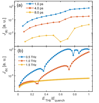
Figure 6: Coherent control of nonlinear dc supercurrent photogeneration. (a) Electric field strength dependence of the THz light-induced dc supercurrent for three different pulse durations with fixed frequency, for fields up to complete quench of the SC order parameter. $E_{\mathrm{quench}}$ denotes the peak electric field needed to completely quench $\Delta$. (b) Electric field strength dependence of $J_{\mathrm{dc}}$ for three different pump frequencies with fixed duration.

Figure 6 demonstrates the nonlinear origin of the symmetry-breaking $J_{\mathrm{dc}}$. The latter can be controlled by tuning the multi-cycle THz field temporal profile, i.e., the number of cycles of oscillation and frequency $\omega_{0}$. Figure 6(a) shows the pump fluence-dependence of the THz-lightwave-induced dc supercurrent for three different pulse durations with fixed $\omega_{0}$. We consider field strengths up to complete quench of the SC order parameter ($E_{\mathrm{quench}}$). The photoinduced $J_{\mathrm{dc}}$, which characterizes the THz dynamical symmetry breaking, increases with decreasing pulse duration, i.e., with fewer cycles of oscillations. In this case, $\int_{-\infty}^{\infty}\mathrm{d}t\,J(t)$ is larger such that the forward and backward propagating electromagnetic fields (35) inside the SC film become more asymmetric which leads to a larger $J_{\mathrm{dc}}$. The pump-frequency dependence of the supercurrent for fixed pulse duration is shown in Fig. 6(b), which demonstrates that $J_{\mathrm{dc}}$ is stronger for the lower-frequency pulses, which again corresponds to fewer cycles of oscillation.

The photogeneration of dc nonlinear supercurrent component and the resulting second harmonic symmetry-forbidden light emission also depend on the bandstructure, especially on the density of states, and can also be controlled by varying the thickness of the SC film Vaswani et al. (2020a). The film thickness dependence of $J_{dc}$ is illustrated in Fig. 7. The latter dependence is dominated by the interference inside the SC film of the light-induced nonlinear current, the incident $E$-field, and the reflected $E$-field, analogous to four-wave mixing. For small film thicknesses, $J_{\mathrm{dc}}$ grows nonlinearly up to roughly 2$\lambda_{0}$, where $\lambda_{0}$ is the wavelength of the pump. In this regime, the region within the SC film where all three waves interfere during the nonlinear dynamics increases with thickness, which results in the increase of the dc supercurrent. With increasing film thickness, the time delay between current and reflected THz lightwave field grows. As a result, the interference between both fields is reduced in some regions within the SC film, due to radiative damping of the current. At the same time, the photoinduced dc supercurrent quenches the SC order parameter. Both effects lead first to a decrease of the dc photocurrent, before $J_{\mathrm{dc}}$ saturates at larger film thicknesses.

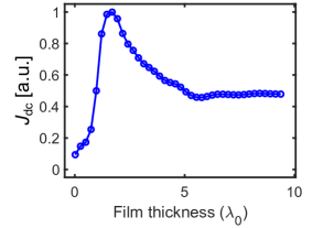
Figure 7: Effect of SC film thickness on dc supercurrent photogeneration for 20 ps-long pump pulse with field strength of 10.0 kV/cm; $\lambda_{0}$ denotes the wavelength of the pump.

VI Nonlinear collective mode phase-coherent spectroscopy

In this section, we focus on the collective mode dynamics of the THz-light-driven SC state. We explore, in particular, ways in which we can control the various dynamical phases that can evolve in time from the SC ground state by tuning the interplay of THz quantum quench, lightwave condensate acceleration, and THz dynamical symmetry breaking. Figure 8(a) shows the changes in the time evolution of the SC order parameter for various pump fields. To characterize the oscillations, we plot the corresponding spectra obtained by Fourier transformation of the order parameter time dependence in Fig. 8(b). Here we show results when the system is driven by a few-cycle 0.5 THz pulse which, as discussed in the previous section, maximizes the $\omega=0$ component of the nonlinear supercurrent. Figure 8(a) demonstrates four different amplitude collective modes selectively excited by such field: (I) In the low excitation regime, $\Delta(t)$ shows damped oscillations (blue line) with frequency $2\Delta_{\infty}>0$. This Higgs amplitude mode Papenkort et al. (2007); Yuzbashyan et al. (2006); Chou et al. (2017) decays as $t^{-1/2}$ (for one-band superconductors) to the steady state order parameter value $\Delta_{\infty}$, as a result of Landau damping due to energy transfer of the collective mode to QPs. $2\Delta_{\infty}=4.2$ meV coincides with the position of the peak in the $\Delta(\omega)$ spectrum (blue line in Fig. 8(b)). (II) By increasing the field strength until we quench the order parameter, $\Delta_{\infty}\approx 0$, we obtain a number of highly nonlinear gapless dynamical phases, whose behavior changes by varying the field strength (Rabi energy) as well as the cycles of oscillation. In regime II, the order parameter displays strong persistent oscillations around the steady state value $\Delta_{\infty}$=0, with multiple frequencies (red line, Fig. 8(b)). This undamped collective mode is due to a synchronization of QP Rabi oscillations excited by the pulse, in a non-equilibrium quantum state with $\Delta_{\infty}=0$ but with a time-dependent coherence Barankov et al. (2004); Collado et al. (2018). (III) Further increase of the pump field amplitude in this highly nonlinear regime with finite condensate momentum leads to excitation of anharmonic damped oscillations of a finite order parameter (yellow line, Fig. 8(a)). The corresponding spectrum (yellow line, Fig. 8(b)) shows a main peak at $0.7$ meV, while high harmonics arise due to the anharmonicity of the order parameter oscillation. This new mode is a consequence of the anisotropic electron and hole distributions driven by the lightwave condensate acceleration, which are displaced in ${\bf k}$ space by ${\bf p}_{\mathrm{S}}(t)$. Such dynamical phase is not accessible by the isotropic order parameter sudden quench or by using the standard Anderson pseudo-spin precession models. In our theory, the electronic distribution is angle-dependent due to THz dynamical symmetry breaking determined by the direction of ${\bf p}_{\mathrm{S}}(t)$, which can be controlled by the lightwave polarization. (IV) In the extreme nonlinear regime, the dynamics becomes over-damped and the order parameter decays exponentially to $\Delta_{\infty}=0$ (purple line, Fig. 8(a)) Yuzbashyan and Dzero (2006); Barankov and Levitov (2006). We conclude that THz dynamical symmetry breaking and ${\bf k}$ space anisotropy controlled via lightwave condensate acceleration allows us to selectively drive dynamical phases (II) and (III), in addition to the familiar phases (I) and (IV). While Phase (II) is also accessible by periodic modulation of Hamiltonian parameters Collado et al. (2018), here we obtain multiple frequencies due to the anisotropic distributions induced by ${\bf p}_{\mathrm{S}}(t)$. Furthermore, the time evolution depends on the synchronization between the pump and Rabi oscillations.

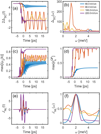
Figure 8: Selective driving of different collective modes of the SC order parameter. (a), (b) Dynamics and spectra of the SC order parameter for various electric field strengths. (c), (d), (e) The corresponding dynamics of the maximum of $\delta\tilde{\rho}_{3}(\mathbf{k})$ among all wavevectors $\mathbf{k}$, the maximum of the QP distributions among all $\mathbf{k}$, and the nonlinear current. (f) The corresponding spectra of the nonlinear current.

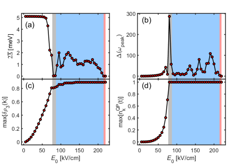
Figure 9: Control of collective amplitude modes by the pump field. Electric field strength dependence of (a) the average value of the order parameter in the non-equilibrium state, $\bar{\Delta}$, (b) the oscillation amplitude of the main peak in $\Delta(\omega)$ spectra, $\Delta(\omega_{\textbf{peak}})$, (c) population inversion $\textrm{max}[\delta\tilde{\rho}_{3}(\mathbf{k})]$, and (d) quasi-particle distribution $\textrm{max}[n^{\textrm{QP}}_{\textbf{k}}]$. Non-equilibrium phase (II) ((III)) is indicated by a gray (blue) shaded area, while phase (IV) is denoted by a red shaded area.

To investigate the systematic lightwave driving of the different non-equilibrium quantum phases, we study the dynamical change of the population inversion $\delta\tilde{\rho}_{3}(\mathbf{k})$, defined in Eq. (A), in more detail. Figure 8(c) shows the dynamics of the maximum of $\delta\tilde{\rho}_{3}(\mathbf{k})$ among all wavevectors $\mathbf{k}$ for the four different dynamical phases in Fig. 8(a). We observe strong population inversion oscillations during the pulse, i.e., Rabi–Higgs oscillations Collado et al. (2018). This population inversion occurs during cycles of lightwave oscillations and defines the initial condition during the pulse for driving collective mode dynamics after the pulse. While for mode (I) $\delta\tilde{\rho}_{3}(\mathbf{k})<0.5$ is small after the pulse, in which case we recover previous non-equilibrium states also obtained within the Anderson pseudo-spin model, phases (II)–(IV) emerge in the extreme nonlinear excitation regime, where the pseudo-spin populations are inverted as compared to the BCS ground state, i.e. $\delta\tilde{\rho}_{3}(\mathbf{k})>0.5$ for some $\mathbf{k}$. To study the emergence of these light-induced dynamical phases by controlling the population inversion in more detail, Fig. 8(d) shows the dynamics of the maximum of the QP distributions among all $\mathbf{k}$, $\textrm{max}[n^{\textrm{QP}}_{\textbf{k}}]$, for the four different phases. For (II)–(IV), THz excitation has created large QP populations with QP distributions close to one, i.e. $\rho_{1,1}^{\mathrm{qp}}(\mathbf{k})=\rho_{2,2}^{\mathrm{qp}}(\mathbf{k})=1$ for some $\mathbf{k}$. These inverted populations remain fully occupied after the pulse for modes (III)–(IV). In particular, as a result of THz dynamical symmetry breaking by ${\bf p}_{\mathrm{S}}(t)$, $\mathbf{k}$-space is separated into two coexisting regions: a SC region and a blocking region. The latter consists of ${\bf k}$ points where Cooper pairs are broken and QP states are fully occupied. The blocking region of ${\bf k}$-space leads to a strong suppression of the anomalous expectation values and the SC order parameter determined by ${\bf p}_{\mathrm{S}}(t)$, such that excitation of collective modes (II)–(IV) becomes possible. The latter is achieved via the anisotropy in ${\bf k}$-space introduced by THz dynamical symmetry breaking for a moving condensate, which results in multiple frequencies for (II) and (III). The dynamical quantum phases driven by the pronounced Rabi–Higgs oscillations modify the light emission spectrum, which makes them experimentally observable. The dynamics and spectra of the nonlinear current $J_{\mathrm{NL}}$ for the four different amplitude modes are shown in Figs. 8(e) and (f). The collective modes (II) and (III) lead to sideband generation around the fundamental harmonic at $\omega_{0}=0.5$ THz. The energy of these sidebands matches the fundamental frequency of the dynamical mode observable in the $\Delta(\omega)$-spectra in Fig. 8(b), so the predicted quantum phases are detectable by looking at the emission spectrum and are controlled by ${\bf p}_{\mathrm{S}}(t)$.

The pump field dependence of the above driven non-equilibrium phases is analyzed in Fig. 9. There we show as a function of the pump field (a) the average value of the order parameter in the non-equilibrium state, $\bar{\Delta}$, and (b) the oscillation amplitude of the main peak in the $\Delta(\omega)$ spectra, $\Delta(\omega_{\textbf{peak}})$. For low pump fields $E_{0}<75$ kV/cm, i.e. prior to strong SC quench, the SC order parameter shows damped oscillations with frequency $2\Delta_{\infty}=2\bar{\Delta}$ (phase (I)). At the same time, the oscillation amplitude monotonically increases analogous to the interaction quench result Yuzbashyan et al. (2006). With increasing $E_{0}$, the system enters dynamical phase (II) (gray shaded area), where $\bar{\Delta}=0$ (quenched SC order) but $\Delta(\omega_{\mathrm{peak}})>0$ (quantum fluctuations). Here, the order parameter shows the strongest oscillation amplitude (quantum fluctuations), i.e the collective mode is amplified (see gray area in Fig. 9(b)). A further increase of $E_{0}$ leads to anharmonic damped oscillations (phase (III), (blue shaded area)) across a wide range of pump fields. For $E_{0}$ exceeding $215$ kV/cm, the system evolves towards phase (IV) (red shaded area) after THz-driven quench where $\bar{\Delta}$=$\Delta(\omega_{\textbf{peak}})$=0. The corresponding field-dependence of the population inversion and QP occupations after the pulse, plotted in Figs. 9(c) and (d), demonstrate that the collective modes (II)–(IV) only emerge in the extreme nonlinear regime, where strong Rabi flopping $\delta\tilde{\rho}_{3}(\mathbf{k})>0.5$ and large QP densities $\rho_{1,1}^{\mathrm{qp}}(\mathbf{k})=\rho_{2,2}^{\mathrm{qp}}(\mathbf{k})=1$ are present.

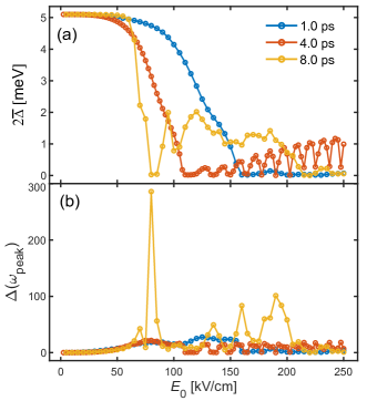
Figure 10: THz temporal profile dependence of driven collective mode phases. Electric field strength dependence of (a) the average value of the order parameter in the non-equilibrium state, $\bar{\Delta}$, and (b) the oscillation amplitude of the main peak in $\Delta(\omega)$ spectra, $\Delta(\omega_{\textbf{peak}})$, for three different pump pulse durations.

The collective modes of the SC order parameter are not only controllable by the pump field strength as above, but also by its temporal profile, i.e., by the cycles of oscillation (frequency and duration) that determine the electromagnetic driving. This is illustrated in Figs. 10(a) and (b), where the pump field dependence of $2\bar{\Delta}$ and $\Delta(\omega_{\textbf{peak}})$ are shown for different number of cycles, obtained by fixing the frequency and varying the excitation duration: $1$ ps (blue line), $4$ ps (red line), and $8$ ps (yellow line). For short pump driving (blue line), the system cannot perform a full Rabi flop required for phases (II) and (III). In this case, one can only access phases (I) and (IV) similar to the sudden quench of the SC order parameter. However, in contrast to sudden quench, $\Delta(\omega_{\textbf{peak}})$ does not monotonically increase within phase (I) up to the transition to phase (IV) (blue line in Fig. 10(b)). In particular, $\Delta(\omega_{\textbf{peak}})$ starts to saturate and then slightly decreases when the pump pulse frequency becomes resonant to $2\Delta(t)$, as the latter deviates from its equilibrium value with time in the non-perturbative regime. Close to the transition to phase (IV), $\Delta(\omega_{\textbf{peak}})$ grows again, before dropping to zero in phase (IV). The situation changes for intermediate excitation durations with increasing number of cycles, in which case phase (III) becomes accessible via Rabi–Higgs oscillations. More specifically, we obtain several transitions between phases (III) and (IV) in the extreme nonlinear regime (red curve). For pulse durations longer than one Rabi flop (8 ps, yellow line), one can also excite phase (II), by adjusting the pump electric field (yellow curve). In this case, we obtain a strong amplification of the Higgs mode strength (yellow curve in Fig. 10(b)) as we quench the order parameter and transition to dynamical phase (II).

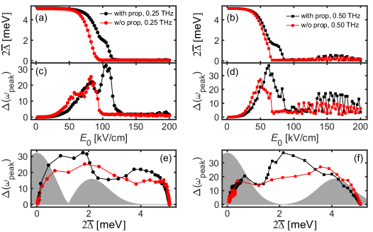
Figure 11: Effect of electromagnetic propagation on collective modes. (a) Electric field strength dependence of the average value of the order parameter in the non-equilibrium state, $\bar{\Delta}$, for a calculation with (black line) and without propagation effects (red line); the SC system has been excited with a 0.25 THz pump field. (c) The corresponding electric field strength dependence of the oscillation amplitude of the main peak in $\Delta(\omega)$ spectra, $\Delta(\omega_{\textbf{peak}})$. (e) $\Delta(\omega_{\textbf{peak}})$ as a function of $2\bar{\Delta}$; the Fourier transform of $E^{2}_{\mathrm{THz}}(t)$ is shown as a shaded area. (b), (d), (f) The corresponding results for a 0.5 THz pump field.

Finally, Figure 11 demonstrates that electromagnetic propagation effects do not only lead to photogeneration of a dc current via THz dynamical symmetry breaking, but can also be used to amplify the oscillation amplitude of the different collective modes. The latter is controlled by the carrier wave cycles of oscillation, which are tuned here by varying the frequency and duration of the applied THz field. We can achieve coherent control by synchronizing the cycles of lightwave oscillations with the SC order parameter and QP dynamics. Figures 11(a) and (c) present the pump field dependence of $2\bar{\Delta}$ and $\Delta(\omega_{\textbf{peak}})$ for the full calculation (black line) and the calculation without electromagnetic propagation effects (red line) for a 0.25 THz pump pulse. Figure 11(e) shows $\Delta(\omega_{\textbf{peak}})$ as a function of $2\bar{\Delta}$, together with the Fourier transform of $E^{2}_{\mathrm{THz}}(t)$ (shaded area). The corresponding results for a 0.5 THz pump pulse are plotted in Figs. 11(b), (d), and (f). Electromagnetic propagation enhances the collective mode oscillations when the pumping, $E_{\mathrm{THz}}^{2}$, is off-resonant with respect to $2\bar{\Delta}$ (Figure 11(e) and (f)). In this case, the finite superfluid momentum $\mathbf{p}_{\mathrm{S}}$ after the pulse leads to a larger blocking region in the anisotropic ${\bf k}$ distribution of pseudo-spins. The condensate motion thus results in much stronger suppression of the anomalous expectation values at certain ${\bf k}$ points in the blocking region. As a result, the amplitude modes of the SC order parameter are more strongly excited, which produces larger oscillation amplitudes (collective mode amplification). The situation changes when $E_{\mathrm{THz}}^{2}$ oscillates at a frequency close to $2\bar{\Delta}$. Here, the lightwave field becomes resonant to $2\Delta$ during the order parameter quench dynamics, such that resonant Higgs mode excitation dominates In particular, the oscillation amplitude is reduced when lightwave propagation is included. We conclude that the Higgs mode can be amplified by lightwave propagation and by tuning the pump frequency.

VII Conclusions

In this paper, we developed a microscopic gauge-invariant density matrix approach and used it to study the non-adiabatic nonlinear dynamics of superconductors driven by lightwave electric fields with few cycles of oscillations. In particular, we generalized the Anderson pseudo-spin precession models used in the literature by non-perturbatively including the Cooper pair’s center-of-mass motion and the condensate spatial variations. We also extended previous SC transport theories by including the non-perturbative coupling of the lightwave oscillating strong field determined by Maxwell’s equations and the nonlinear photocurrent, which we showed can break inversion symmetry after the pulse, thus leading to gapless non-equilibrium SC and new collective modes. The obtained gauge-invariant SC Bloch equations, together with Maxwell’s wave equation, describe the nonlinear dynamical interplay between lightwave acceleration of the Cooper-pair condensate, Anderson pseudo-spin nonlinear precession, QP Rabi oscillations as well as population inversion, spatial dependence, and electromagnetic pulse propagation effects. Our theory allows us to treat both amplitude and phase dynamics, driven during cycles of lightwave oscillations, in a gauge-invariant way. Such theory can be extended to treat topological phase ultrafast dynamics.

We have applied the above comprehensive model to demonstrate that coherent nonlinearities driven by realistic few-cycle THz laser pulses, together with lightwave propagation effects inside a nonlinear SC thin film system, can photogenerate a nonlinear supercurrent with a dc component. Such nonlinear supercurrent breaks the equilibrium inversion symmetry of the SC system, which can be detected experimentally via high-harmonic generation at equilibrium-forbidden frequencies, formation of gapless SC non-equilibrium phases, and Rabi–Higgs collective modes with amplitude amplification. The above nonlinear effects can be tuned, e.g., by adjusting the thickness of the SC film and the cycles of lightwave oscillation. We have also shown that THz driven Rabi–Higgs flopping and population inversion for sufficiently strong fields can selectively excite and coherently control different classes of collective modes of the SC order parameter. More specifically, we have shown that, with lightwave condensate acceleration, one can access, in the extreme nonlinear excitation regime, damped harmonic and anharmonic order parameter amplitude oscillations, persisting oscillations, and an overdamped phase. Differences from quantum quench of the SC order parameter studied before arise since the THz electric field breaks inversion symmetry of electron and hole distributions due to lightwave acceleration of the condensate during cycles of oscillation. We thus obtain order-parameter oscillations with multiple frequencies, leading to controllable and broad high harmonic generation. In particular, the lightwave-driven damped anharmonic oscillating mode (phase III) and persisting oscillations (phase II) modify the light emission spectrum by producing sideband generation around the fundamental harmonic. Finally we have demonstrated that lightwave propagation inside the SC film can significantly amplify the collective mode oscillations. Such amplification also occurs by driving phase II of persisting order parameter oscillations, i.e., quantum fluctuations due to synchronized Rabi oscillations at the threshold field for quenching the SC order parameter to zero.

The theoretical approach presented here is not restricted to BCS superconductors with a single order parameter. It can be extended, for example, to study the THz-driven non-equilibrium dynamics in multi-band superconductors, in SC systems with multiple coupled order parameters, such as iron-based superconductors Patz et al. (2014, 2017), or in $d$-wave or topological SCs that can be tuned via ${\bf p}_{\mathrm{S}}(t)$. In this connection, one expects to see a rich spectrum of non-equilibrium phases and phase/amplitude collective modes in the non-equilibrium SC dynamics and the extreme nonlinear optics regime, to be explored elsewhere. As possible new directions, the derived Bloch–Maxwell equations can be applied to study lightwave propagation effects in SC metamaterials, as well as to analyze and predict new multi-dimensional THz coherent nonlinear spectroscopy experiments in superconductors and topological materials. For example, in SCs, such experiments provide a way to distinguish between charge-density fluctuations and collective mode signatures, study quantum interference and nonlinear wave-mixing effects in quantum states, and generate light-controlled collective mode hybridization. Topological order also leads to analogous effects determined by the quantum mechanical phase, to be studied elsewhere. Phase dynamics in SCs can play an important role when spatial variations are considered. We conclude that THz dynamical symmetry breaking during cycles of coherence oscillations is a powerful concept for addressing quantum sensing and coherent control of different quantum materials Li et al. (2013); Patz et al. (2015); Kapetanakis et al. (2009); Chovan et al. (2006); Chovan and Perakis (2008); Lingos et al. (2015); Liu et al. (2020) and topological phase transitions Luo et al. (2019); Yang et al. (2020) at the ultimate sub-cycle speed limit necessary for lightwave quantum electronics and magneto-electronics.

Appendix A Radiative damping

To study the radiative damping predicted by our theory, we express the density matrix $\tilde{\rho}(\mathbf{k})$ in terms of the Anderson pseudo-spins at each ${\bf k}$ point,

$$\tilde{\rho}(\mathbf{k})=\sum_{n=0}^{3}\tilde{\rho}_{n}(\mathbf{k})\sigma_{n}\,,$$ (37)

where $\sigma_{n}$ are the Pauli spin matrices and

$$\tilde{\rho}_{0}=\frac{\tilde{\rho}_{1,1}(\mathbf{k})+\tilde{\rho}_{2,2}(\mathbf{k})}{2}\,,\quad\tilde{\rho}_{1}=\frac{\tilde{\rho}_{1,2}(\mathbf{k})+\tilde{\rho}_{2,1}(\mathbf{k})}{2}\,,$$

$$\tilde{\rho}_{2}=\mathrm{i}\frac{\tilde{\rho}_{1,2}(\mathbf{k})-\tilde{\rho}_{2,1}(\mathbf{k})}{2}\,,\quad\tilde{\rho}_{3}=\frac{\tilde{\rho}_{1,1}(\mathbf{k})-\tilde{\rho}_{2,2}(\mathbf{k})}{2}\,,$$ (38)

are the components of the Anderson pseudo-spin. The equations of motion of the pseudo-spin components are

$$\frac{\partial}{\partial t}\tilde{\rho}_{0}(\mathbf{k})=-e\mathbf{E}\cdot\nabla_{\mathbf{k}}\tilde{\rho}_{3}(\mathbf{k})-2|\Delta|\sum_{n=0}^{\infty}\frac{(\mathbf{p}_{\mathrm{S}}\cdot\nabla_{\mathbf{k}})^{2n+1}}{(2n+1)!}\tilde{\rho}_{2}(\mathbf{k})\,,$$

$$\frac{\partial}{\partial t}\tilde{\rho}_{1}(\mathbf{k})=\left[\xi(\mathbf{k}-\mathbf{p}_{\mathrm{S}})+\xi(\mathbf{k}+\mathbf{p}_{\mathrm{S}})-2\,\mu_{\mathrm{eff}}-2\mu_{\mathrm{F}}\right]\tilde{\rho}_{2}(\mathbf{k})\,,$$

$$\frac{\partial}{\partial t}\tilde{\rho}_{2}(\mathbf{k})=-\left[\xi(\mathbf{k}-\mathbf{p}_{\mathrm{S}})+\xi(\mathbf{k}+\mathbf{p}_{\mathrm{S}})-2\,\mu_{\mathrm{eff}}-2\mu_{\mathrm{F}}\right]\tilde{\rho}_{1}(\mathbf{k})$$

$$\qquad+2|\Delta|\sum_{n=0}^{\infty}\left[\frac{(\mathbf{p}_{\mathrm{S}}\cdot\nabla_{\mathbf{k}})^{2n}}{(2n)!}\tilde{\rho}_{3}(\mathbf{k})-\frac{(\mathbf{p}_{\mathrm{S}}\cdot\nabla_{\mathbf{k}})^{2n+1}}{(2n+1)!}\tilde{\rho}_{0}(\mathbf{k})\right]\,,$$

$$\frac{\partial}{\partial t}\tilde{\rho}_{3}(\mathbf{k})=-e\mathbf{E}\cdot\nabla_{\mathbf{k}}\tilde{\rho}_{0}(\mathbf{k})+2|\Delta|\sum_{n=0}^{\infty}\frac{(\mathbf{p}_{\mathrm{S}}\cdot\nabla_{\mathbf{k}})^{2n}}{(2n)!}\tilde{\rho}_{2}(\mathbf{k})\,.$$ (39)

We then linearize the equations of motion (A) with respect to deviations from equilibrium yielding

$$\frac{\partial}{\partial t}\delta\tilde{\rho}_{0}(\mathbf{k})=-e\mathbf{E}\cdot\nabla_{\mathbf{k}}\tilde{\rho}_{3}^{(0)}(\mathbf{k})\,,$$

$$\frac{\partial}{\partial t}\delta\tilde{\rho}_{1}(\mathbf{k})=2\xi(\mathbf{k})\delta\tilde{\rho}_{2}(\mathbf{k})\,,$$

$$\frac{\partial}{\partial t}\delta\tilde{\rho}_{2}(\mathbf{k})=2\xi(\mathbf{k})\delta\tilde{\rho}_{1}(\mathbf{k})-2\delta\mu_{\mathrm{eff}}\tilde{\rho}_{1}^{(0)}$$

$$\qquad+2\Delta_{0}\delta\tilde{\rho}_{3}(\mathbf{k})+2\delta\Delta\tilde{\rho}_{3}^{(0)}(\mathbf{k})\,,$$

$$\frac{\partial}{\partial t}\delta\tilde{\rho}_{3}(\mathbf{k})=2\Delta_{0}\delta\tilde{\rho}_{2}(\mathbf{k})\,,$$ (40)

where

$$\delta\tilde{\rho}_{n}(\mathbf{k})=\tilde{\rho}_{n}(\mathbf{k})-\tilde{\rho}^{(0)}_{n}(\mathbf{k})\,,\quad\delta\mu_{\mathrm{eff}}=\frac{\mathrm{i}}{2}\frac{\partial}{\partial t}\theta+e\phi+\delta\mu_{\mathrm{F}}\,,$$

$$\delta\delta\mu_{\mathrm{F}}=g\sum_{\mathbf{k}}\delta\tilde{\rho}_{3}(\mathbf{k})\,,\quad\delta\Delta=\Delta(t)-\Delta_{0}\,,$$ (41)

with equilibrium pseudo-spin components

$$\tilde{\rho}^{(0)}_{0}(\mathbf{k})=1\,,\quad\tilde{\rho}^{(0)}_{1}(\mathbf{k})=\frac{\Delta_{0}}{\sqrt{\xi(\mathbf{k})^{2}+\Delta_{0}^{2}}}\,,$$

$$\tilde{\rho}^{(0)}_{2}(\mathbf{k})=0\,,\quad\tilde{\rho}^{(0)}_{3}(\mathbf{k})=-\frac{\xi(\mathbf{k})}{\sqrt{\xi(\mathbf{k})^{2}+\Delta_{0}^{2}}}\,.$$ (42)

Here we applied perturbation theory with respect to linear order in the electric field $\mathbf{E}$, i. e. we have neglected all contributions of order $\mathcal{O}(\mathbf{E}^{2})$ and higher. We next Fourier transform Eq. (A) and insert the result into the Fourier transformation of the current (23). By combining the result with the Fourier transformation of Eq. (35), we find

$$|J(\omega)|^{2}=4n^{2}\varepsilon_{0}^{2}\Gamma^{2}\frac{|\mathbf{E}_{0}(\omega)|^{2}}{\omega^{2}+\Gamma^{2}}\,,$$ (43)

where we introduced the radiative coupling constant

$$\Gamma=\frac{e^{2}}{S\hbar^{2}}\frac{1}{2n\varepsilon_{0}c}\sum_{\mathbf{k}}\frac{\partial}{\partial k_{x}}\xi(\mathbf{k})\frac{\partial}{\partial k_{x}}\tilde{\rho}_{3}^{(0)}(\mathbf{k})\,,$$ (44)

after assuming that the applied electric field $\mathbf{E}_{0}$ is polarized in $x$-direction. The self-consistent coupling between the photoexcited current and the lightwave field thus induces a radiative damping, which is given by Eq. (44) in linear order perturbation theory.

The transformation from particle space to quasi-particle space is performed using the unitary Bogoliubov transformation

$$\rho^{\mathrm{qp}}(\mathbf{k})=\mathcal{U}_{\mathbf{k}}\,\tilde{\rho}(\mathbf{k})\,\mathcal{U}_{\mathbf{k}}^{\dagger}\,,\quad\mathcal{U}_{\mathbf{k}}=\begin{pmatrix}u_{\mathbf{k}}&v_{\mathbf{k}}\\ -v_{\mathbf{k}}&u_{\mathbf{k}}\end{pmatrix}\,,$$ (45)

with coherence factors

$$u_{\mathbf{k}}=\sqrt{\frac{1}{2}\left(1+\frac{\varepsilon_{\mathbf{k}}}{E_{\mathbf{k}}}\right)}\,,\quad v_{\mathbf{k}}=\sqrt{\frac{1}{2}\left(1-\frac{\varepsilon_{\mathbf{k}}}{E_{\mathbf{k}}}\right)}\,,$$ (46)

where

$$\varepsilon_{\mathbf{k}}=\frac{\xi(\mathbf{k}+\mathbf{p}_{\mathrm{S}}/2)+\xi(\mathbf{k}-\mathbf{p}_{\mathrm{S}}/2)}{2}\,,\quad E_{\mathbf{k}}=\sqrt{\varepsilon_{\mathbf{k}}^{2}+|\Delta|^{2}}\,.$$ (47)

Here we have chosen an instantaneous quasi-particle basis with time-dependent coherence factors (46), which diagonalizes the time-dependent homogeneous Hamiltonian. The corresponding quasi-particle energies are given by

$$E^{\mathrm{qp}}_{\mathbf{k},\pm}=\frac{\xi(\mathbf{k}+\mathbf{p}_{\mathrm{S}}/2)-\xi(\mathbf{k}-\mathbf{p}_{\mathrm{S}}/2)}{2}\pm E_{\mathbf{k}}\,.$$ (48)