Reinforcement Learning Control of Robotic Knee with Human in the Loop by Flexible Policy Iteration

Abstract

We are motivated by the real challenges presented in a human-robot system to develop new designs that are efficient at data level and with performance guarantees such as stability and optimality at systems level. Existing approximate/adaptive dynamic programming (ADP) results that consider system performance theoretically are not readily providing practically useful learning control algorithms for this problem; and reinforcement learning (RL) algorithms that address the issue of data efficiency usually do not have performance guarantees for the controlled system. This study fills these important voids by introducing innovative features to the policy iteration algorithm. We introduce flexible policy iteration (FPI), which can flexibly and organically integrate experience replay and supplemental values from prior experience into the RL controller. We show system level performances including convergence of the approximate value function, (sub)optimality of the solution, and stability of the system. We demonstrate the effectiveness of the FPI via realistic simulations of the human-robot system. It is noted that the problem we face in this study may be difficult to address by design methods based on classical control theory as it is nearly impossible to obtain a customized mathematical model of a human-robot system either online or offline. The results we have obtained also indicate the great potential of RL control to solving realistic and challenging problems with high dimensional control inputs.

I Introduction

Robotic knees are wearable robots that assist individuals with lower limb amputation to regain the ability of walking [1, 2]. This type of robotic prosthesis relies on mimicking how biological joints generate torques to enable the robotic knee motion for an amputee user. The device is programmed to adjust the knee joint impedance values according to the mechanical sensors in the prosthesis. The intrinsic controllers embedded in the devices provide baseline automatic control of joint torques. As human users differ from weight to size and are of different life-style needs, extrinsic control in the form of providing impedance parameter settings are required to customize the device to meet individual user’s physical and life style needs.

Related Approaches. While such new powered device signifies the future of rehabilitation, and it has brought excitement into the biomechanics fields, fitting the device to a human user automatically remains a major challenge to unleash the full potential of the robotic device. Few technologies are currently available. The only functioning solution relies on multiple sessions of manually tuning a small subset of the impedance parameters one at a time, unable to account for the interacting effects of the parameters during each tuning session. This highly heuristic approach is time consuming, costly, and not scalable to reaching the full potential of this powerful robotic device.

Some research has gone into reducing the intensity of labor for parameter tuning. One such idea directly reduces the number of configurable parameters [3, 4]. In return, significant domain knowledge and tuning time are still required, and it is not clear if such an approach will remain effective for each unique individual of the amputee population. In [5], an expert system was developed to hard code the prosthetists’ tuning decisions into configuring the control parameters. This open-loop control approach is not expected to scale well to more joints or to more tasks. Other approaches include estimating the control impedance parameters with either a musculoskeletal model [6] or measurements of biological joint impedance [7, 8]. These methods have not been validated and it is questionable if they are feasible as the biomechanics and the joint activities of amputees are fundamentally different from those of the able-bodied population. A recent continuous tracking approach was proposed based on extremum seeking, aka a convex optimization solution, for seeking impedance parameters [9]. The idea applied as a concept to knee and ankle joints by automatically tuning the proportion gain of a PD controller. It is yet to see direct results of leg motion performance either in simulation or by human testing.

As those methods all have their fundamental limitations in principled ways, new approaches of configuring the prosthesis control parameters are needed. Even though controlling exoskeleton is not quite the same problem as configuring prosthesis control parameters because of the fundamental and physiological differences between able-bodied and amputee populations, it is still worth mentioning that several optimization techniques have been proposed for the former. In [10], the authors used gradient descent method to determine an optimal control onset time of an ankle exoskeleton device. Their goal was to minimize the metabolic effort from respiratory measurements and thus improve gait efficiency. The authors of [11] also studied ankle exoskeleton towards minimizing the metabolic effort, where in the study, they used an evolution strategy to optimize four control parameters in the ankle device. Ding et al. [12] applied Bayesian optimization to place two control parameters of hip extension assistance. While this idea and those discussed are interesting for exoskeleton, they may not extend to robotic prosthesis parameter tuning problem as these algorithms have only been demonstrated for less or equal to a 5-dimensional control parameter space. In addition to scalability, they have not shown feasibility in addressing challenges such as adapting to user’s changing physical condition or change in use environments. Additionally, the metabolic cost objective used in control design of exoskeletons for able bodied individuals is unlikely useful for amputees using a prosthetic device.

Problem Challenges. Several unique characteristics of the human-robot system are responsible for the challenges we face when configuring the robotic devices. First, fundamental principles and mechanisms of how the human and prosthesis interact still is not known. Therefore, it is not feasible to apply control design approaches that rely on a mathematical description of the human-prosthesis dynamics. Second, lower limb prosthesis tuning is commonly implemented in a finite state machine impedance control (FS-IC) framework [13] because studies have suggested that humans actually control the joint impedance of the leg when walking [14, 15]. The FS-IC involves multiple configurable parameters or control inputs, from 12 to 15 for knee prosthesis for level ground walking [1, 2, 16], and the number of parameters grows rapidly for increased number of joints and locomotion modes up to multiple dozens. Third, the impedance control design has to ensure the safety and stability of the human user at all times. Additionally, because of a human user is in the loop during the tuning process, it is highly desirable for the control design approach to be data and time efficient to reduce the discomfort caused by adjusting the control parameters. Addressing these challenges simultaneously requires us to look beyond classical control systems theory and control systems engineering as well as the state-of-the-art robotics science and engineering that have been successful at controlling mechanical robots.

Reinforcement Learning and Adaptive Dynamic Programming. The reinforcement learning (RL) based adaptive optimal control is naturally appealing to solve the above described challenges. As is well known, deep RL, including several policy search methods and Deep Q-Network (DQN), have shown unprecedented successes in solving difficult, sequential decision-making problems, such as those in robotics applications [17], Atari games [18], the game of Go [19, 20] and energy efficient data center [21]. Yet, a few challenges remain if these results are to be extended to situations where there is no abundance of data, the problems involve continuous state and control variables, uncertainties as well as sensor and actuator noise are inevitable, and system performances such as optimality and stability have to be satisfied. RL based adaptive optimal control approaches, or adaptive/approximate dynamic programming (ADP) [22, 23], is a promising alternative as they have demonstrated their capability of learning from data measurements in an online or offline manner in several realistic application problems including large-scale control problems, such as power system stability enhancement [24]-[26], and Apache helicopter control [27, 28]. Note however, those problems do not face the data and time efficiency challenge.

At the heart of the ADP methods is the idea of providing approximating solutions to the Bellman equation of optimal control problems. In our previous work [29]-[31], we demonstrated the feasibility of ADP, specifically direct heuristic dynamic programming (dHDP) [32], for personalizing robotic knee control, to address similar challenges we face here. The dHDP is an online RL algorithm based on stochastic gradient descent, which in its generic form, is not optimized for fast learning [33]. It is also worth mentioning that, the generic dHDP without imposing further conditions [34] have not shown its control law to be stable during learning. It is therefore necessary to take these limitations into design considerations especially for the current application.

Policy Iteration RL Control. AlphaGo Zero [20] is a policy iteration-based reinforcement learning algorithm. It started tabula rasa, achieved superhuman performance after only a few days of training. This result is inspiring. Yet, how to make a classic policy iteration algorithm applicable to solving controls problem that requires data and time efficiency as well as system stability and optimal performance remains a challenge. ADP is a promising adaptive optimal control framework to address general nonlinear control problems. But few results are available to demonstrate successful applications to real controls problems while meeting the data and time efficiency requirements. Some motivating and important theoretical works are as follows, but they do not directly involve data-level design approaches to solving realistic and complex problems. In [35]-[37], the authors examined continuous time systems of different constraining nonlinearity forms (affine systems, for example) under respective state and control conditions. For discrete-time systems, [38] deals with a class of linear systems, [39] deals with an affine nonlinear system with learning convergence proof, [40] deals with nonlinear systems with learning convergence proof and optimality performance, However, system stability was not provided in [39, 40]. Stable iterative control policies of PI have been studied in [41]-[44] for discrete-time nonlinear systems of different forms. However, only within the generic PI formulation without any consideration of integrating prior knowledge. Clearly, we need a practical, data level design algorithm that is useful for applications while retaining important, system level performance properties such as optimality and stability.

Using Prior Information. Two design ideas to account for data and time efficiency are intuitively useful – experience replay and value function shaping. We innovatively develop both ideas and organically integrate them into our FPI algorithms.

Experience replay (ER) [45] is a practically effective approach to improving sample efficiency for off-policy RL methods. In ER, past experiences (samples) generated under different behavior policies are stored in a memory buffer and selected repeatedly for evaluating the approximated value function. Even though ER has been adopted and analyzed extensively, shown below, current results do not simultaneously fulfill our design requirement of data level efficiency and performance guarantee simultaneously. Empirical studies have demonstrated successes of several ER algorithms. Selective experience replay (SER) [46], prioritized experience replay (PER) [47, 48] and hindsight experience replay (HER) [49] have shown their capability in improving sample efficiency in deep RL. Specifically, SER strategically selects which experiences will be stored so that the distribution on the memory buffer can match the global distribution in the training dataset. In contrast, PER selects which experiences to be replayed in the memory buffer. That is to say, the important samples will be replayed more frequently. For multi-goal RL, HER reutilizes past failure experiences which may benefit for another goal, so that the overall multi-goal performance can be improved.The ER idea has also been considered in ADP in different capacities [50]-[56]. Beyond the results in [45]-[49], the works in [50] and [51] also empirically demonstrated that the simple experience replay idea, without prioritization or other means of selecting samples, can be implemented with Q-learning and actor-critic ADP algorithms to improve sample efficiency. Some analytical studies [52]-[56] about ER have carried out for specific systems and under specific conditions, which are not sufficiently general to be applied to our human-robot system. Specifically, ER, or concurrent learning, was proposed to replace the persistence of excitation (PE) condition for uncertain linear dynamical systems [52], partially unknown constrained input systems [53], known deterministic nonlinear systems [54], non-zero sum games based on model identifiers of the game systems [55] and decentralized event-triggered control of interconnected systems in affine form with uncertain interconnections [56]. Apparently, existing results are not readily extended to address the challenges just discussed in the above.

The idea of using prior experience to bootstrap learning is intuitive as it intends to capture knowledge from a related task to help save data and learning time. Research has shown significant improvement in data and time efficiency by using prior experience as compared to learning from scratch [57, 58, 59]. At present, most approaches rely on identifying and applying a good initial policy or initial value function to “guide” learning in order to reduce the policy search space as a means of reducing data complexity and saving learning time [60, 61, 62, 63]. A handful of results attempted formal treatment of utilizing prior knowledge to boost learning, yet they are only for special considerations. [64] is an early work that considered boosting the value function or shaping the reward function. But the focus was to ensure policy invariance, not from a perspective of saving data and training time. [65] provided a theoretical sample complexity framework, yet it is unclear how the results could directly impact the development of practically useful algorithms. [58] proved a probably approximately correct (PAC) guarantee for a scheme that uses an optimistic value function initialization, and the authors only demonstrated their approach using simple examples.

Contributions and Significance. From the above discussions, it is clear that practical, data level design algorithms with important, system level performance properties are still lacking. In this study, we introduce flexible policy iteration (FPI) to address the challenges. The flexibility of our proposed FPI is within the following three aspects. First, the way it collects and uses data, i.e., data preparation (Table I), to permit learning from samples generated from either current behavior policies or different policies within an experience replay framework. Second, the way it deals with prior knowledge is flexible as it allows learning from prior knowledge in the form of a supplemental value based on previous data collection experiments. Third, the implementation of FPI is flexible as the approximate value function can be obtained by a conventional least-square solution or by a weighted least-square solution with or without prioritized samples. With such a flexible framework, a designer of an adaptive optimal controller can customize his/her algorithmic approach to fit specific applications needs.

In summary, we are motivated by the real challenges presented in a human-robot system to develop new designs that are efficient at data level and with performance guarantees at systems level. Successful applications of policy iteration, such as AlphaGo Zero, are inspiring but did not account for either data efficiency or system stability. Existing ADP results that consider system performance theoretically are not readily providing practically useful learning control algorithms. This study fills these important voids. Specifically, our contributions are as follows.

• First, based on the classic policy iteration framework, we introduce several flexibilities at data level, each or all of which can be customized to meet the design and problem solving needs. Our innovative development of experience replay and supplemental values, and organic integration of them into the policy evaluation, have provided practically useful design tools.

• Second, we not only introduce FPI as an iterative learning procedure, but we also provide qualitative analysis of FPI for its stabilizing control laws, convergence of the value function and achieving Bellman optimality approximately.

• Third, we provide extensive simulation studies to validate what we intended for the FPI: to automatically configure 12 impedance parameters as prosthesis control inputs to enable continuous walking of amputee subjects.

It is noted that, what we have obtained in this study would have been difficult or impossible for designs based on classic control theory. Our results reported here represent the state of the art in automatic configuration of powered prosthetic knee devices. This result may potentially lead to practical use of the FPI in clinics. In turn, this can significantly reduce health care cost and improve the quality of life for the transfemoral amputee population in the world.

The remaining of this paper is organized as follows. Section II describes the human-prosthesis system and formulates the human-prosthesis tuning/configuration problem. Section III presents the FPI framework for online control of prosthetic knee. Section IV analyzes the converging properties of FPI. Section V presents the experimental results of the FPI-tuner under different configurations, and a comprehensive comparison to other existing RL methods. Discussions and conclusion are presented in Section VI.

II Human-Robot System

In this study, RL is applied to automatically adjust impedance parameter settings within a finite state impedance control (FS-IC) framework, where a gait cycle is divided into four phases to represent different modes of stance and swing [1, 7, 16] (Fig. 1(b)): stance flexion phase (STF, $m=1$), stance extension phase (STE, $m=2$), swing flexion (SWF, $m=3$) and swing extension (SWE, $m=4$). Transitions between phases are triggered by the ground reaction force (GRF), knee joint angle, and knee joint angular velocity measured from the prosthesis. Variance in a certain phase will affect the subsequent phases [66]. Fig. 1(a) shows an FS-IC based human-prosthesis system and how our proposed reinforcement learning control is integrated into the system. There are two control loops running at different frequencies. The intrinsic, impedance control (IC) loop generates knee joint torque $T$ at 300 Hz following the impedance control law (2), given an impedance control parameter setting defined in (1). For each of the gait phases $m=1,2,3,4,$ there is a respective FPI controller. In each gait cycle $k$ for each phase $m$, state $x_{k}$ is formed using peak knee angle $P_{k}$ and gait phase duration $D_{k}$ measures as shown in Fig. 1(b).

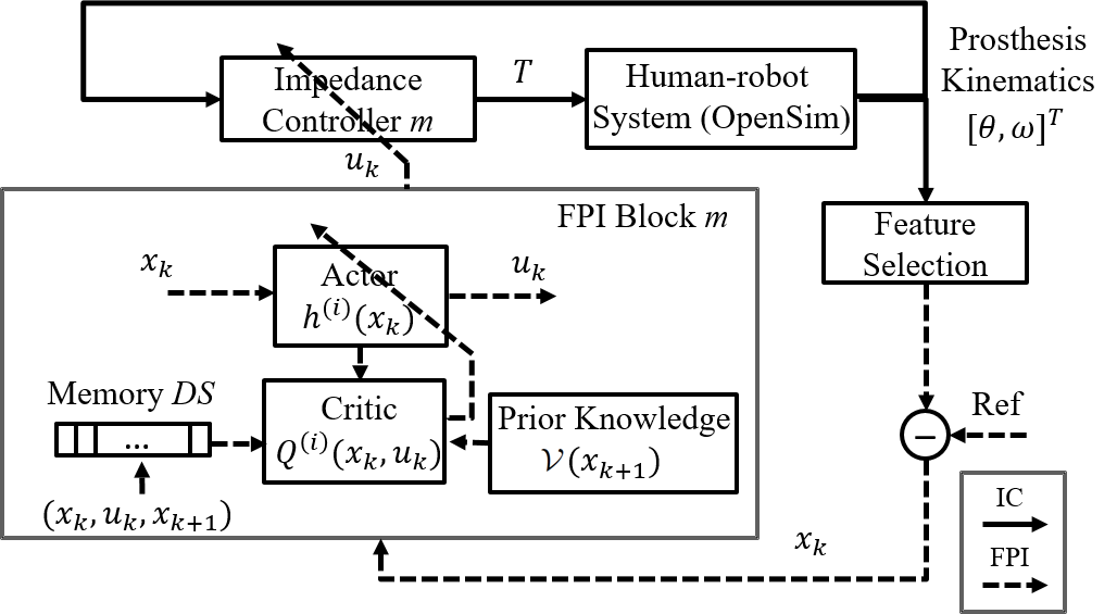
(a)

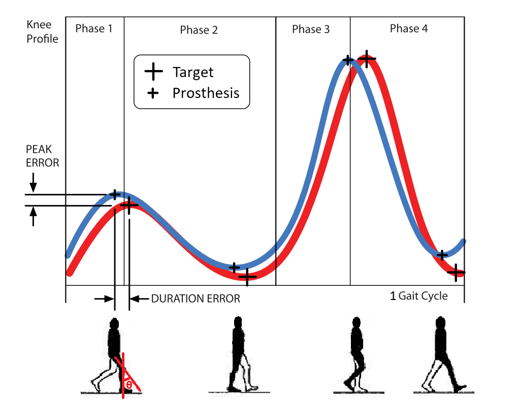
(b)

Figure 1: (a) Block diagram of the human-robot system with a RL controlled robotic knee. The impedance control loop (IC loop, top) generates torque $T$ according to (2). The FPI-based parameter update loop (FPI loop) adjusts impedance control parameters for each phase $m$ after every gait cycle $k$. Four identical RL blocks ($m=1,2,3,4$) are needed for the four IC control phases. (b) Illustration of the four phases of a gait cycle: the differences between the target and prosthesis knee profiles form the states peak error and duration error of the four respective phases.

II-A The Intrinsic Impedance Control Loop

Refer to the top IC control loop of Fig. 1(a). During gait cycle $k$, for each FS-IC control phase $m$ $(m=1,2,3,4)$, robotic knee control requires three control parameters, namely stiffness $K_{m,k}$, damping coefficient $B_{m,k}$ and equilibrium position $(\theta_{e})_{m,k}$. In vector form, the control parameter settings are represented as

$$I_{m,k}=[K_{m,k},B_{m,k},(\theta_{e})_{m,k}]^{T}\in\mathbb{R}^{3}.$$ (1)

The prosthetic knee motor generates a knee joint torque $T\in\mathbb{R}$ from the knee joint angle $\theta$ and angular velocity $\omega$ according to the following impedance control law

$$T_{k}=K_{k}(\theta-(\theta_{e})_{k})+B_{k}\omega.$$ (2)

Without loss of generality, we drop the subscript $m$ in the rest of the paper because all four impedance controllers and their respective FPI blocks share the same structure, although RL controller for each phase has its own coefficients to generate impedance control settings (1). The FPI controller then updates the IC parameter settings (1) for the next gait cycle $k+1$ as

$$I_{k+1}=I_{k}+u_{k},$$ (3)

where $u_{k}\in\mathbb{R}^{3}$ is the control input generated from the FPI block.

II-B Impedance Parameter Update Loop by FPI

Refer to the bottom control loop of Fig. 1(b). For each phase $m$ during gait cycle $k$, the $m$th FPI controllers is enabled to update the IC parameters. After each gait cycle $k$, the peak knee angle $P_{k}\in\mathbb{R}$ and phase duration $D_{k}\in\mathbb{R}$ are selected by the feature selection module. Specifically, peak knee angle $P_{k}$ is the maximum or minimum knee angle in each phase, and phase duration $D_{k}$ is the time interval between two consecutive peaks (Fig. 1(b)). A reference trajectory of the knee joint that resembles a normal human walking pattern [1, 67] is used in this study. Subsequently we can also determine target peak angle $P_{k}^{{}^{\prime}}\in\mathbb{R}$ and phase duration $D_{k}^{{}^{\prime}}\in\mathbb{R}$. For each RL controller in a respective phase, its state variable $x_{k}$ is defined using peak error $\Delta P_{k}\in\mathbb{R}$ and duration error $\Delta D_{k}\in\mathbb{R}$ as

$$x_{k}=[\text{$\Delta$}P_{k},\text{$\Delta$}D_{k}]{}^{T}=[P_{k}-P_{k}^{{}^{\prime}},D_{k}-D_{k}^{{}^{\prime}}]{}^{T},$$ (4)

and its control $u_{k}$ consists of increments to the IC parameters,

$$u_{k}=[\Delta K_{k},\Delta B_{k},(\text{$\Delta$}\theta_{e}\text{)}{}_{k}]^{T}.$$ (5)

III Flexible Policy Iteration

Consider the human-robot, i.e., the amputee-prosthesis, system as a discrete time nonlinear system with unknown dynamics,

$$x_{k+1}=F(x_{k},u_{k}),\hphantom{}k=0,1,2,\text{\ldots}$$ (6)

where action $u_{k}$ of the form described in (5) is determined according to policy $h$ as

$$u_{k}=h(x_{k}).$$ (7)

In (6), the domain of $F(x_{k},u_{k})$ is denoted as $\mathcal{D}\triangleq\{(x,u)|x\in\mathfrak{\mathcal{X}},u\in\mathcal{U}\}$, where $\mathcal{X}$ and $\mathcal{U}$ are compact sets with dimensions of $N_{x}$ and $N_{u}$, respectively. In the human-robot system under consideration, $F$ represents the kinematics of the robotic knee, which is affected by both the human wearer and also the RL controller. Because of a human in-the-loop, an explicit mathematical model as (6) is intractable or impossible to obtain.

III-A The Policy Iteration Framework

To assist our development of the proposed flexible policy iteration (FPI), we summarize the notation and the basic framework of a standard policy iteration algorithm for discrete time systems next.

The RL control design objective is to derive an optimal control law via learning from observed data along the human-robot system dynamics. Consider a control policy $h(x_{k})$, we define the state-action Q-value function as

$$\check{Q}(x_{k},u_{k})=\check{U}(x_{k},u_{k})+\sum_{j=1}^{\infty}\check{U}(x_{k+j},h(x_{k+j}))$$ (8)

where $\check{U}(x_{k},u_{k})$ is the stage cost or instantaneous cost function. Note that the $\check{Q}(x_{k},u_{k})$ value is a performance measure when action $u_{k}$ is applied at state $x_{k}$ and the control policy $h$ is followed thereafter. The form of $\check{Q}(x_{k},u_{k})$ in (8) implies that we formulate the optimal control problem of robotic knee as a discrete time, infinite horizon and undiscounted optimization problem. Our solution framework is data-driven, not model-based.

Our design approach requires the following assumption.

Assumption 1.

The system $F(x_{k},u_{k})$ (6) is controllable; the system state $x_{k}=0$ is an equilibrium state of system (6) under the control $u_{k}=0$, i.e., $F(0,0)=0$; the feedback control $u_{k}=h(x_{k})$ satisfies $u_{k}=h(x_{k})=0$ for $x_{k}=0$; the stage cost function $\check{U}(x_{k},u_{k})$ in $x_{k}$ and $u_{k}$ is positive definite.

Assumption 1 is satisfied in the robotic knee control problem due to our construction of the system states and RL control (3) based on the biomechanics of human locomotion.

The Q-value function in (8) satisfies the following Bellman equation,

$$\check{Q}(x_{k},u_{k})=\check{U}(x_{k},u_{k})+\check{Q}(x_{k+1},h(x_{k+1})).$$ (9)

An optimal control is the one that stabilizes the system in (6) while minimizing the value function (8) according to Bellman optimality. The optimal value function is therefore of the form

$$Q^{*}(x_{k},u_{k})=\check{U}(x_{k},u_{k})+\underset{u_{k+1}}{\min}Q^{*}(x_{k+1},u_{k+1})$$ (10)

or

$$h^{*}(x_{k})=\underset{u_{k}}{\arg\min}Q^{*}(x_{k},u_{k}),$$ (11)

$$Q^{*}(x_{k},u_{k})=\check{U}(x_{k},u_{k})+Q^{*}(x_{k+1},h^{*}(x_{k+1})),$$ (12)

where $h^{*}(x_{k})$ denotes the optimal control policy.

Consider an iterative value function $\check{Q}^{(i)}(x_{k},u_{k})$ and a control policy $\check{h}^{(i)}(x_{k})$, the policy iteration algorithm proceeds by iterating the follow two steps for $i=0,1,2,\ldots$:

Policy Evaluation

$$\check{Q}^{(i)}(x_{k},u_{k})= \check{U}(x_{k},u_{k})+\check{Q}^{(i)}(x_{k+1},\check{h}^{(i)}(x_{k+1})).$$ (13)

The above policy evaluation step (13) is based on the Bellman equation (9).

Policy Improvement

$$\check{h}^{(i+1)}(x_{k})=\underset{u_{k}}{\arg\min}\check{Q}^{(i)}(x_{k},u_{k}).$$ (14)

Motivated by the favorable properties of policy iteration in MDP problems, such as monotonically decreasing value, and demonstrated feasibility in solving realistic engineering problems [25, 26], we further develop the policy evaluation step to achieve data efficiency, easy implementation, and importantly, effectively solving realistic and complex problems.

III-B Flexible Policy Iteration with Supplemental Value

We first consider a flexible use of prior information, which we expect to improve learning efficiency in data and time. Our approach entails a supplemental value $\mathcal{V}(x_{k})$ which can be obtained from an FPI solution based on past experience such as a robotic knee control experiment involving a similar subject(s) previously. For $i=0,1,2,\ldots$ we define a new augmented cost-to-go $Q^{(i)}(x_{k},u_{k})$ based on a supplemental value $\mathcal{V}(x_{k})$,

$$Q^{(i)}(x_{k},u_{k})= \check{U}(x_{k},u_{k})+\sum_{j=1}^{\infty}\check{U}(x_{k+j},h^{(i)}(x_{k+j}))$$ (15)

$$+\sum_{j=0}^{\infty}\alpha_{i}\mathcal{V}(x_{k+j}).$$

We need the following assumption.

Assumption 2.

The supplemental coefficient $\alpha_{i}$ satisfies $0\leq\alpha_{i+1}<\alpha_{i}<1,$ and $\lim_{i\rightarrow\infty}\alpha_{i}=0.$ $\mathcal{V}(x_{k})$ in (15) is finite and positive definite in $x_{k}$.

Note that the major difference between $Q^{(i)}(x_{k},u_{k})$ in (15) and the original $\check{Q}^{(i)}(x_{k},u_{k})$ in (13) is an extra term $\sum_{j=0}^{\infty}\alpha_{i}\mathcal{V}(x_{k+j})$. In fact, (15) can be rewritten as

$$Q^{(i)}(x_{k},u_{k})= \check{U}(x_{k},u_{k})+\alpha_{0}\mathcal{V}(x_{k})$$ (16)

$$+\sum_{j=1}^{\infty}[\check{U}(x_{k+j},h^{(i)}(x_{k+j}))+\alpha_{i}\mathcal{V}(x_{k+j})].$$

We can see that the stage cost $\check{U}(x_{k},u_{k})$ is supplemented by $\mathcal{V}(x_{k})$. This augmented value $Q^{(i)}(x_{k},u_{k})$ is no longer the same as $\check{Q}^{(i)}(x_{k},u_{k})$ in the regular formulation of policy iteration (13). With this additional supplemental value, the learning agent receives guidance to shape the sequence of stage costs $\check{U}$.

With such an augmented Q-value formulation in (16), the policy evaluation step (13) and policy improvement step (14) becomes:

Policy Evaluation with Supplemental Value

$$Q^{(i)}(x_{k},u_{k})= U^{(i)}(x_{k},u_{k})+Q^{(i)}(x_{k+1},h^{(i)}(x_{k+1}))$$

$$,i=0,1,2,\ldots$$ (17)

where $U^{(i)}(x_{k},u_{k})=\check{U}(x_{k},u_{k})+\alpha_{i}\mathcal{V}(x_{k}).$

Policy Improvement

$$h^{(i+1)}(x_{k})=\underset{u_{k}}{\arg\min}Q^{(i)}(x_{k},u_{k}),i=0,1,2,\ldots$$ (18)

Remark 1.

The term $\mathcal{V}$ represents a supplemental value obtained from a previous experiment where $\mathcal{V}(x_{k})=\underset{u_{k}}{\min}Q_{f}(x_{k},u_{k})$. In the above, $Q_{f}(x_{k},u_{k})$ is a converged value function from applying a naive FPI without any supplemental value $\mathcal{V}$ (Algorithm 1) or just PI. The supplemental value $\mathcal{V}(x_{k})$ so formulated from a previous experiment of a similar human subject can capture essential information represented in the value $\mathcal{V}$ for state $x_{k}$. When this information is used in a new experiment, the $Q^{(i)}(x_{k},u_{k})$ value has previously obtained information embedded into the current learning. Note, however, that both experiments must use the same stage cost and cost-to-go function constructs.

Similar to regular policy evaluation (13) and (14), we need the following assumption for the initial control law $h^{(0)}(x)$ in (17) and (18):

Assumption 3.

The initial control law $h^{(0)}(x)$ is admissible.

Definition 1.

(Admissible Control [41]) : A control policy $h(x)$ is admissible with respect to the value function $\check{Q}(x,u)$ (15) if $h(x)$ is continuous on $\mathcal{X}$, $h(0)=0$ and it stabilizes system (6), and the corresponding value function $\check{Q}(x,u)$ (15) is finite for $\forall x\in\mathcal{X}$.

An initially feasible set of impedance control parameters are available from the prosthesis manufacturers and/or trained technicians/experimenters who can customize the prosthesis for individual patients. After all, manual tuning of the impedance parameters is the current practice in clinics. In Theorem 3, given an initially admissible control law $h^{(0)}(x)$, we will show that the iterative control law $h^{(i)}(x)$ is also admissible for $i=1,2,\ldots$ .

Solving (17) and (18) to obtain closed-form optimal solutions $Q^{*}(x_{k},u_{k})$ and $h^{*}(x_{k})$ are difficult or nearly impossible. A value function approximation (VFA) scheme replaces the exact value function in (17) with a function approximator such as neural networks. Such approximation based approaches to solving the Bellman equation, or RL approaches, usually utilize an actor-critic structure where the critic evaluates the performance of a control policy and the actor improves the control policy based on the critic evaluation. Both the actor and the critic work together iteratively and learning takes place forward-in-time to approximately solve the Bellman equation.

Our next strategy to improve policy evaluation efficiency is to innovatively utilize experience replay.

III-C Flexible Sampling with Experience Replay

In policy evaluation (17), the value function $Q^{(i)}$ is to be evaluated with multiple samples of $s_{k}=(x_{k},u_{k},x_{k+1})$. How many samples to use and how to select the samples directly impact policy evaluation. We propose the following options to flexibly select the number of samples and/or prioritize the samples in order to improve policy evaluation.

Let $DS=\{s_{k}\}_{N}$ of size $N$ be a memory buffer. When there is no abundance of data, it would be natural to perform a policy evaluation of (17) using not only newly available sample but also all those samples already in the memory buffer $DS$ which may include off-policy samples, on-policy samples, or both.

Next, samples in $DS$ can be assigned with different priorities so that the important samples are more likely to be reused. In this work, the importance of sample $s_{k}$ is measured by the temporal difference (TD) error from a transition [47], which indicates how surprising or unexpected the transition is: specifically, how far the value is from its next-step bootstrap estimate.

Let $\delta_{k}^{(i)}$ be the TD error of sample $s_{k}$ in $DS$ under policy $h^{(i)}$. The rank $\zeta_{k}^{(i)}$ (ordinals from 1, which corresponds to the largest TD error) of sample $s_{k}$ is obtained from sorting the memory buffer $DS$ according to $|\delta_{k}^{(i)}|$ in a descending order. Then each sample $s_{k}$ is assigned a weight $\bar{\lambda}_{k}^{(i)}$ as

$$\bar{\lambda}_{k}^{(i)}=\frac{1}{\zeta_{k}^{(i)}},\textrm{for }\forall k,$$ (19)

and $\bar{\lambda}_{k}^{(i)}$ can be normalized to a value between 0 and 1 as

$$\lambda_{k}^{(i)}=\frac{\bar{\lambda}_{k}^{(i)}}{\sum\bar{\lambda}_{k}^{(i)}},\textrm{for }\forall k.$$ (20)

The $\lambda_{k}^{(i)}$ can then provide a flexibility for weighing the samples when solving the Bellman equation.

III-D Approximate Policy Evaluation with Flexibility

To implement the policy evaluation step (17), a function approximator $\hat{Q}^{(i)}(x_{k},u_{k})$ is used for $Q^{(i)}(x_{k},u_{k})$. We use a universal function approximator such that:

$$\hat{Q}^{(i)}(x_{k},u_{k})=W^{(i)T}\phi(x_{k},u_{k})=\sum_{j=1}^{L}w_{j}^{(i)}\varphi_{j}(x_{k},u_{k})$$ (21)

where $W^{(i)}\in\mathbb{R}^{L}$ is a weight vector and $\phi(x_{k},u_{k}):\mathbb{R}^{N_{x}}\times\mathbb{R}^{N_{u}}\rightarrow\mathbb{R}^{L}$ is a vector of the basis functions $\varphi_{j}(x_{k},u_{k}),k=1\ldots L$. The basis functions $\varphi_{j}(x_{k},u_{k})$ can be neural networks, polynomial functions, radial basis functions, etc. In our implementations (Section V), we employ polynomial basis, the associated universal approximation property can be shown by the Stone-Weierstrass theorem.

The policy evaluation step (17) then becomes

$$\hat{Q}^{(i)}(x_{k},u_{k})$$ (22)

$$=U^{(i)}(x_{k},u_{k})+\hat{Q}^{(i)}(x_{k+1},h^{(i)}(x_{k+1})).$$

Substituting (21) into (22), we have

$$W^{(i)T}[\text{$\phi$}(x_{k},u_{k}) -\text{$\phi$}(x_{k+1},h^{(i)}(x_{k+1}))]$$ (23)

$$=U^{(i)}(x_{k},u_{k}).$$

Equation (22) can be seen as an approximated policy evaluation step in terms of a weight vector that is to be determined from solving $L$ linear equations. At iteration $i$, two column vectors $X^{(i)}\in\mathbb{R}^{N\text{\texttimes}L}$ and $Y^{(i)}\in\mathbb{R}^{N}$, are formed by the term $\text{$\phi$}(x_{k},u_{k})-\text{$\phi$}(x_{k+1},h^{(i)}(x_{k+1}))$ and $U^{(i)}(x_{k},u_{k})$, respectively, in each row. In other words, (23) can be rewritten as

$$W^{(i)T}X^{(i)}=Y^{(i)}.$$ (24)

The TD error $\delta_{k}^{(i)}$ can be computed as

$$\delta_{k}^{(i)}= U^{(i)}(x_{k},u_{k})+\hat{Q}^{(i-1)}(x_{k+1},h^{(i)}(x_{k+1}))$$ (25)

$$-\hat{Q}^{(i-1)}(x_{k},u_{k}),\textrm{for }i=0,1,2,\ldots$$

Then the weight $\lambda_{k}^{(i)}$ of a sample can be obtained from (20). For $i=0$, assign weights $\lambda_{k}^{(0)}=1$. When the policy evaluation with function approximation (22) is carried out with sample $s_{k}=(x_{k},u_{k},x_{k+1}),$ it can be weighted by $\lambda_{k}^{(i)}$. Hence, the weight vector $W^{(i)}$ can be computed from (24) as a weighted least squares solution using $N$ weighted samples

$$W^{(i)}=(X^{(i)^{T}}\Lambda^{(i)}X^{(i)}){}^{\dagger}(X^{(i)^{T}}\Lambda^{(i)}Y^{(i)})^{T},$$ (26)

where $\Lambda^{(i)}\text{$\in$}\mathbb{R}^{N}$ is a vector of $\lambda_{k}^{(i)}$ and ^† is the Moore-Penrose pseudoinverse. Once $W^{(i)}$ is obtained, the approximated value function $\hat{Q}^{(i)}(x_{k},u_{k})$ can be obtained using (21).

Note that, in (24) to (26) we use $N$ samples to estimate the weight vector $W^{(i)}\in\mathbb{R}^{L}.$ For $\hat{Q}^{(i)}$ to be convergent, we need the following PE-like condition.

Condition 1.

The vector $X^{(i)}$ formed by $N$ samples in $DS$ contains as many linear independent elements as the unknown parameters in the weight vector $W^{(i)}$, i.e., $rank(X^{(i)})=L$.

Remark 2.

The number of samples $N$ in the memory buffer can be fixed or adaptive with $N>L$ satisfied necessarily. Unlike PE, Condition 1 can be checked in real time easily. Adding a small Guassian noise (for example, 1% of initial impedance value) to the impedance values $u_{k}=h^{(i)}(x_{k})$ suffices for meeting Condition 1.

Algorithm 1 Flexible Policy Iteration (FPI)

Initialization by

Random initial state $x_{0}\in\mathfrak{\mathcal{X}}$, initial batch size $N_{b}$ (if in batch mode), memory buffer $DS=\emptyset$, initially admissible control policy $h^{(0)}$. Let the approximated policy $\hat{h}^{(0)}=h^{(0)}.$

Data Preparation for Iteration $i$

1a: (Batch Data Collection) Collect $N_{b}$ samples $\{(x_{k},u_{k},x_{k+1})\}_{N_{b}}$ from system (6) following policy $\hat{h}^{(i)}$from gait cycle $k$, $N\leftarrow N_{b}$ (Setting 2(A) in Table I).

1b: (Incremental Data Collection) Collect a sample $(x_{k},u_{k},x_{k+1})$ from system (6) following policy $\hat{h}^{(i)}$, and add it to $DS$, $N\leftarrow N+1$ (Setting 2(B) in Table I).

2: (Set Batch Size) Either use a fixed or adaptive $N_{b}$ (Setting 1 in Table I) if under batch mode (Setting 2(A) in Table I).

3: (Set Other Parameters) Determine $\lambda_{k}^{(i)}$ (Setting 3 in Table I) and $\alpha_{i}$ (Setting 4 in Table I).

Policy Evaluation/Update for Iteration $i$

4: (Policy Evaluation) Evaluate policy $\hat{h}^{(i)}$ by solving (22) for $\hat{Q}^{(i)}$ using (26), for example, and by using all samples in $DS$.

5: (Policy Update) Update policy $\hat{h}^{(i+1)}$ by (28) and (29).

TABLE I: Data Preparation and Parameter Settings in Algorithm 1

Setting		Description
1	(A) $N_{b}$ is fixed	Fixed
	(B) $N_{b}\leftarrow N_{b}+5$	Adaptive
2	(A) $N\leftarrow N_{b}$	Batch mode
	(B) $N\leftarrow N+1$	Incremental mode
3	(A) $\lambda_{k}^{(i)}=1$	No prioritization
	(B) $\lambda_{k}^{(i)}$ from (20)	With prioritization
4	(A) $\alpha_{i}=0$	No supplemental value
	(B) $\alpha_{i}=0.9^{i}$	With supplemental value

III-E Policy Improvement in FPI

After the approximated value function $\hat{Q}^{(i)}(x_{k},u_{k})$ is obtained, the next policy $h^{(i+1)}(x_{k})$ from (18) is,

$$h^{(i+1)}(x_{k})=\underset{u_{k}}{\arg\min}\hat{Q}^{(i)}(x_{k},u_{k}).$$ (27)

We employ another linear-in-parameter universal function approximator $\hat{h}^{(i+1)}(x_{k})$ for $h^{(i+1)}(x_{k})$,

$$\hat{h}^{(i+1)}(x_{k})=(\mathcal{K}^{(i+1)})^{T}\sigma(x_{k}),$$ (28)

where $\mathcal{K}^{(i+1)}$ is a weight vector and $\sigma(x_{k})$ is a basis function vector. The weight vector $\mathcal{K}^{(i+1)}$ is updated iteratively using the gradient of the approximate value function $\hat{Q}^{(i)}(x_{k},u_{k})$,

$$\mathcal{K}_{j+1}^{(i+1)}=\mathcal{K}_{j}^{(i+1)}-l\dfrac{\partial\hat{Q}^{(i)}(x_{k},(\mathcal{K}_{j}^{(i+1)})^{T}\sigma(x_{k}))}{\partial\mathcal{K}_{j}^{(i+1)}}$$ (29)

where $l$ is the learning rate ($0<l<1$), $j$ is the iteration step within a policy iteration step.

III-F Implementation of FPI

Algorithm 1 and Table I together describe our proposed FPI algorithm. The terminating condition in Algorithm 1 can be, for example, policy iteration index $i=i_{max}$ where $i_{max}$ is some positive number, or $|\hat{Q}^{(i)}(x_{k},u_{k})-\hat{Q}^{(i-1)}(x_{k},u_{k})|<\varepsilon$ where $\varepsilon$ is a small positive number. Note that there are four settings in Algorithm 1 (Table I). FPI can run in batch mode or incremental mode (Setting 2). In batch mode, only samples (of length $N_{b}$) generated under the same policy are used in policy evaluation, thus no sample reuse is allowed in this mode. In incremental mode, previous samples of length $N$ in the $DS$ that are generated under different policies, plus a newly acquired sample, can be reused to evaluate a new policy. In batch mode, an extra parameter batch size $N_{b}$ need to be set (Setting 1 in Table I), while such parameter is not required under incremental mode. In addition, Setting 3 describes how the priorities $\lambda_{k}^{(i)}$ of the samples are assigned and Setting 4 describes how the supplemental value is used at iteration $i$ through the parameter of $\alpha_{i}$ .

Note that in batch mode, FPI can choose the number of samples for policy evaluation adaptively. FPI starts with a small $N_{b}$. A newly generated policy is tested with one or more gait cycles to determine if the policy can lower the stage cost. If not, a larger set of samples (e.g. $N_{b}\leftarrow N_{b}+5$) is used.

This adaptive approach is based on our observations as follows. Given a continuous state and control problem such as the control of a robotic knee, we constructed a quadratic stage cost $(x_{k},u_{k})$ in (52) which is common in control system design. As a decreasing stage cost can be viewed as necessary toward an improved value during each iteration, it thus becomes a natural choice for such a selection criterion. For example, Fig. 2 depicts stage cost for the uniformly sampled IC parameter space in our human-robot application, where the color of each sample point represents a stage cost. Fig. 3 was generated under the setting of (A)(A)(A)(A) in Table I and $N_{b}=20$. Fig. 3 shows the trajectories of the IC parameters tuned by FPI starting from some random initial IC parameters. Apparently, the points with minimum stage cost in Fig. 2 coincides with the converging planes found by FPI in Fig. 3.

IV Qualitative Properties of FPI

Policy iteration based RL has been shown possessing several important properties, such as convergence of policy iteration, approximately reaching Bellman optimality, and stabilizing control [40], [41]-[44]. We now address the question of whether these properties still hold under our proposed FPI framework especially when our formulation includes a supplemental value.

Lemma 1.

Let $i=0,1,...$ be the iteration number and let $Q^{(i)}(x_{k},u_{k})$ and $h^{(i)}(x_{k})$ be updated by (17)-(18). Under Assumption 1, the stage cost $U^{(i)}(x_{k},u_{k})$ and iterative value function $Q^{(i)}(x_{k},u_{k})$ in (17) are positive definite for $x_{k}$ and $u_{k}$.

Proof:

For $i=0$, according to Assumption 1, we have $h^{(0)}(x_{k})=0$ as $x_{k}=0$. As $\check{U}(x_{k},u_{k})$ is positive definite for $x_{k}$ and $u_{k}$, we have that $\sum_{j=0}^{\infty}\check{U}(x_{k+j},h^{(0)}(x_{k+j}))=0$ as $x_{k}=0,$ and $\sum_{j=0}^{\infty}\check{U}(x_{k+j},h^{(0)}(x_{k+j}))>0$ for any $x_{k}\neq 0$. Hence $\sum_{j=0}^{\infty}\check{U}(x_{k+j},h^{(0)}(x_{k+j}))$ is a positive definite function for $x_{k}$. Since $\mathcal{V}(x_{k})$ is also positive definite for $x_{k}$, it is easy to get $U^{(i)}(x_{k},u_{k})$ is positive definite for $x_{k}$ and $u_{k}$. According to (15), if $x_{k}=u_{k}=0$, $Q^{(0)}(x_{k},u_{k})=0$; if $|x_{k}|+|u_{k}|\neq 0$, $Q^{(0)}(x_{k},u_{k})>0$, which proves that $Q^{(0)}(x_{k},u_{k})$ is positive definite for $x_{k}$ and $u_{k}.$ Based on this idea, we can prove that the iterative function $Q^{(i)}(x_{k},u_{k}),i=0,1,...,$ is positive definite for $x_{k}$ and $u_{k}.$ ∎

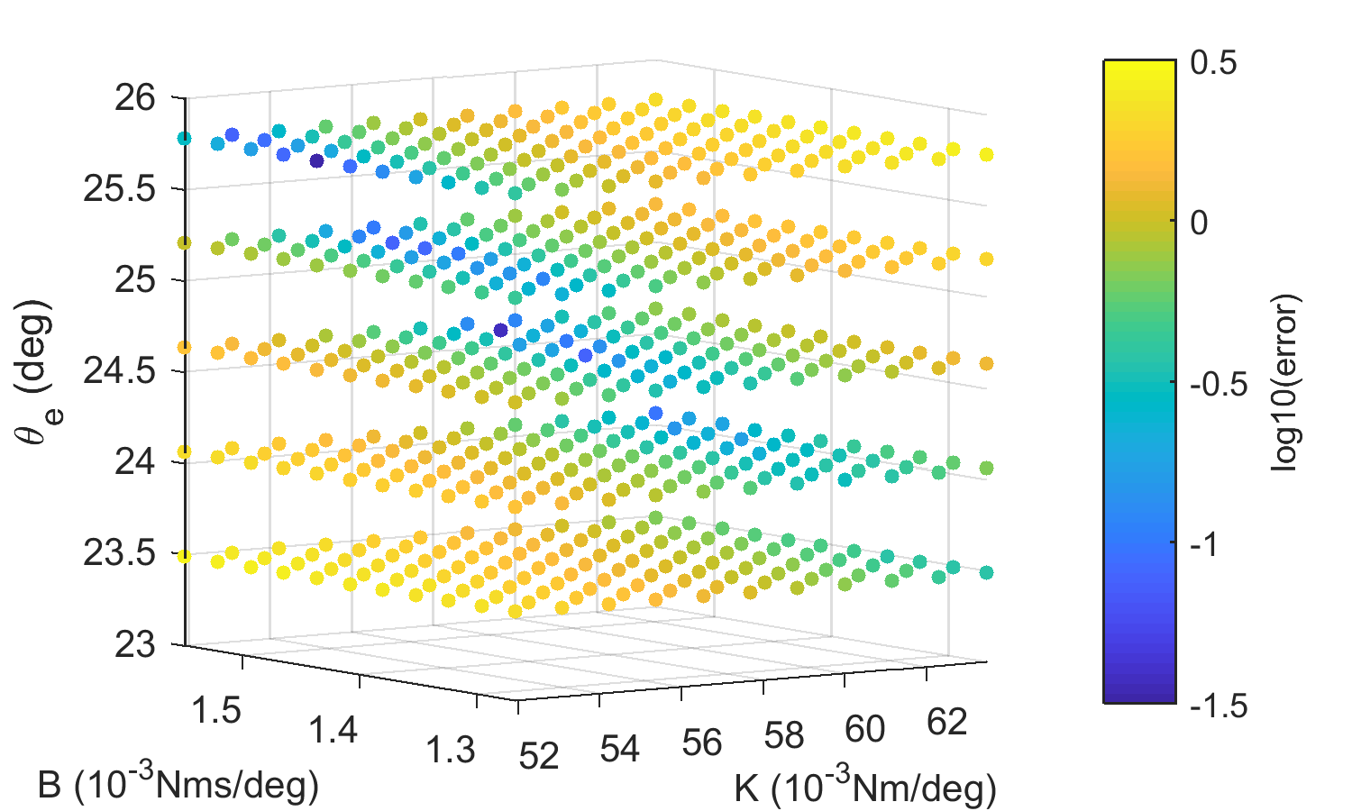
(a) Phase 1

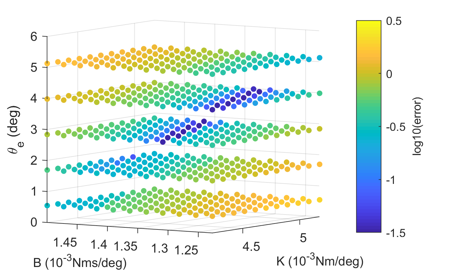
(b) Phase 2

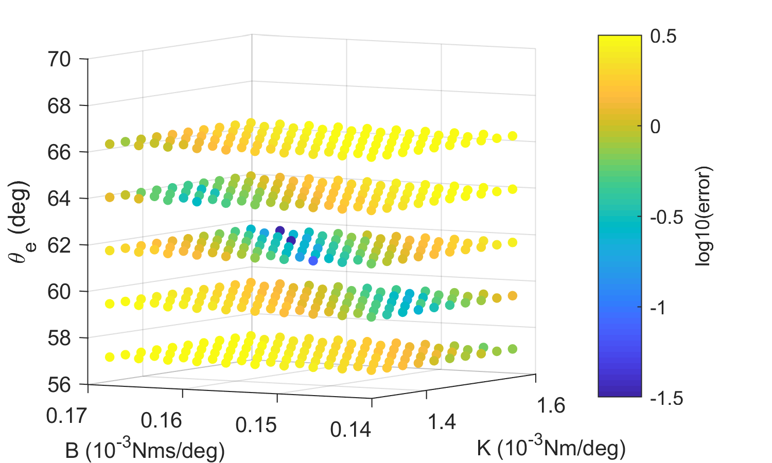
(c) Phase 3

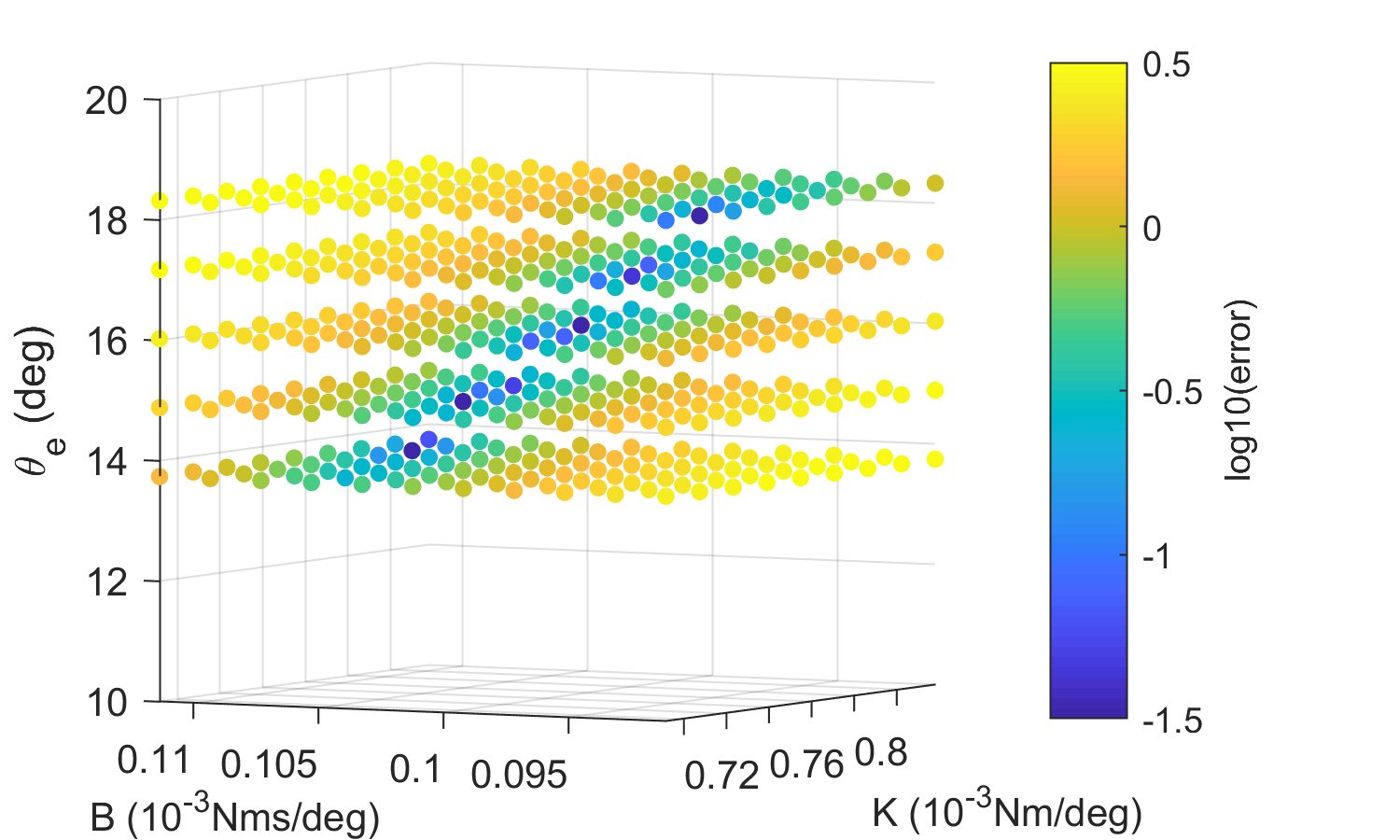
(d) Phase 4

Figure 2: The stage cost in peak error and duration error as in equation (52).

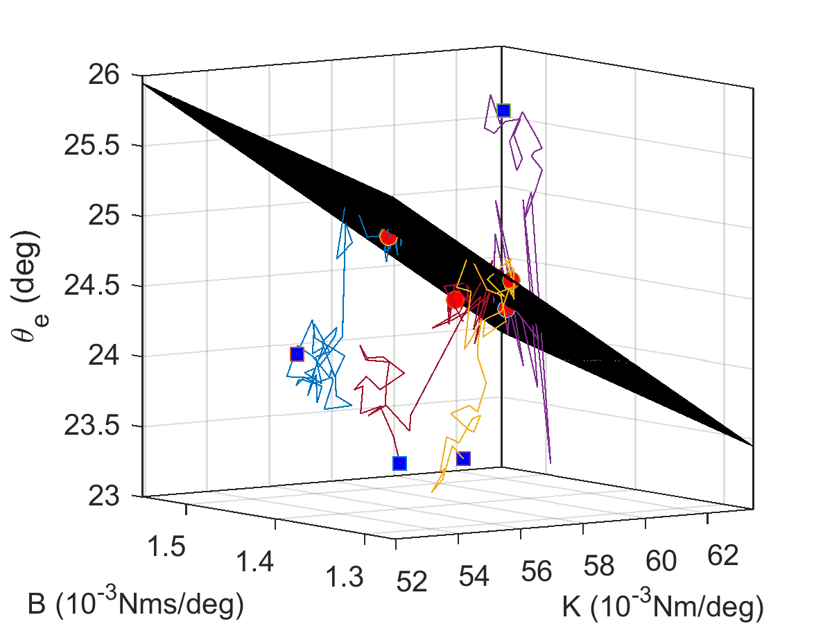
(a) Phase 1

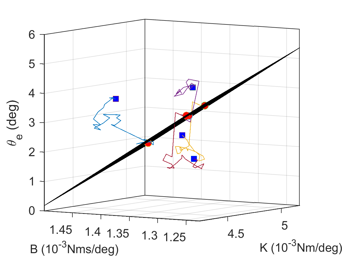
(b) Phase 2

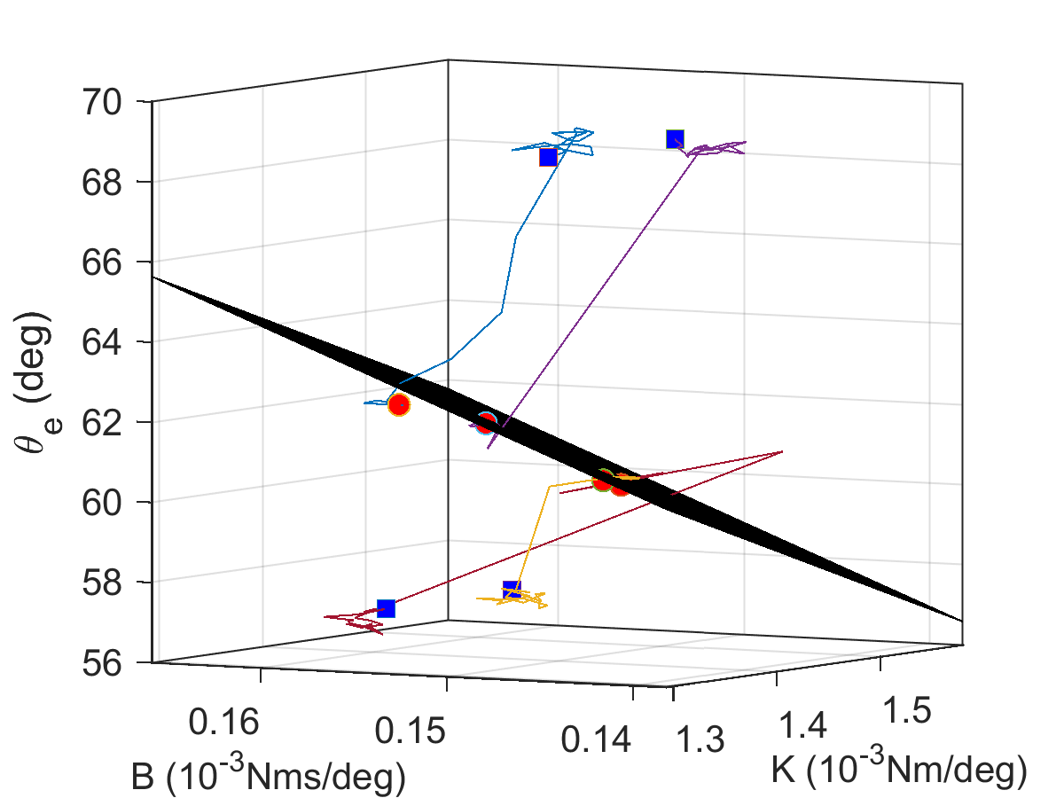
(c) Phase 3

(d) Phase 4

Figure 3: Illustration of the converging process of the IC parameters during FPI tuning: from randomly initialized IC parameters (four trials for illustration here, shown in blue squares) to the final parameters (shown in red dots), which are fitted with a regression response surface.

Theorem 1.

Let Assumptions 1-3 hold. Let $Q^{(i)}(x_{k},u_{k})$ and $h^{(i)}$ be updated by (17)-(18). Then, for $i=0,1,2,...,$ $h^{(i)}$ stabilizes the system (6).

Proof:

Consider the case when $x_{k}\neq 0$, we have $U^{(i)}(x_{k},h^{(i)}(x_{k}))>0$ and $\alpha_{i}(x_{k+1})\geq 0.$ From (17), and $i=0,1,\ldots,$

$$Q^{(i)}(x_{k},h^{(i)}(x_{k}))-Q^{(i)}(x_{k+1},h^{(i)}(x_{k+1}))$$ (30)

$$=U^{(i)}(x_{k},h^{(i)}(x_{k}))>0.$$

Next, consider the case when $x_{k}=0$, according to Assumption 1 we can get $h^{(i)}(x_{k})=0$ and thus $U^{(i)}(x_{k},h^{(i)}(x_{k}))=0$, which imply $Q^{(i)}(x_{k},h^{(i)}(x_{k}))-Q^{(i)}(x_{k+1},h^{(i)}(x_{k+1}))=0.$ According to Lemma 1 and Assumption 1, the function $Q^{(i)}(x_{k},h^{(i)}(x_{k}))$ is positive definite for $x_{k}$. Then $Q^{(i)}(x_{k},h^{(i)}(x_{k}))$ is a Lyapunov function. Thus $h^{(i)}$ stabilizes the system (6). ∎

Remark 3.

Theorem 1 shows that the Lyapunov stability can be guaranteed under iterative policy $h^{(i)}(x_{k})$ under the augmented value formulation of (15). Additionally, embedded safety constraints on the knee joint angles and angular velocities [31] ensure the states and the controls are within the domain $D$ of the system dynamics $F(x_{k},u_{k})$ in (6). Human subjects are therefore guaranteed to be practically stable.

Theorem 2.

Let Assumptions 1-3 hold. Let the value function $Q^{(i)}(x_{k},u_{k})$ and the control policy $h^{(i)}(x_{k})$ be obtained from (17) and (18), respectively. Then $Q^{(i+1)}(x_{k},u_{k})\leq Q^{(i)}(x_{k},u_{k})$ holds for $i=0,1,2,\ldots$ and $\forall(x_{k},u_{k})\in\mathcal{D}.$

Proof:

For convenience, we will use the following short hand notations in the derivations, e.g., $U^{(i)}(x_{k},h^{(i)})$ for $U^{(i)}(x_{k},h^{(i)}(x_{k}))$. According to (15), we can define $V(x_{k})$ as

$$V^{(i)}(x_{k})=Q^{(i)}(x_{k},h^{(i)})=\sum_{j=k}^{\infty}U^{(i)}(x_{j},h^{(i)}).$$ (31)

Based on (18), we have

$$Q^{(i)}(x_{k},h^{(i+1)}) =\underset{u_{k}}{\min}Q^{(i)}(x_{k},u_{k})$$

$$\leq Q^{(i)}(x_{k},h^{(i)}).$$ (32)

Based on (17) we have

$$V^{(i)}(x_{k}) =Q^{(i)}(x_{k},h^{(i)})$$

$$\geq Q^{(i)}(x_{k},h^{(i+1)})$$

$$=U^{(i)}(x_{k},h^{(i+1)})+V^{(i)}(x_{k+1})$$

$$\geq U^{(i)}(x_{k},h^{(i+1)})+V^{(i)}(x_{k+1}).$$ (33)

Hence

$$V^{(i)}(x_{k})-V^{(i)}(x_{k+1}) \geq U^{(i)}(x_{k},h^{(i+1)})$$

$$V^{(i)}(x_{k+1})- V^{(i)}(x_{k+2})$$

$$\geq U^{(i)}(x_{k+1},h^{(i+1)})$$

$$\vdots$$

$$V^{(i)}(x_{k+L})- V^{(i)}(x_{k+L+1})$$

$$\geq U^{(i)}(x_{k+L},h^{(i+1)}).$$ (34)

Summing up the left and the right hand sides of (34) respectively,

$$V^{(i)}(x_{k})- V^{(i)}(x_{k+L+1})$$ (35)

$$\geq\sum_{j=k}^{k+L}U^{(i)}(x_{j},h^{(i+1)})$$

$$\geq 0,$$

where $L$ is a positive integer corresponding to gait cycles in this paper. Hence, (35) yields

$$V^{(i)}(x_{k})\geq V^{(i+1)}(x_{k}).$$ (36)

According to (17) and (36), we can obtain

$$Q^{(i+1)}(x_{k},u_{k}) =U^{(i)}(x_{k},u_{k})+V^{(i+1)}(x_{k+1})$$

$$\leq U^{(i)}(x_{k},u_{k})+V^{(i)}(x_{k+1})$$

$$=Q^{(i)}(x_{k},u_{k}).$$ (37)

∎

Theorem 3.

Let Assumptions 1-3 hold. Let $Q^{(i)}(x_{k},u_{k})$ and $h^{(i)}$ be updated by (17)-(18), respectively. Then for $i=0,1,2,\ldots,$ $h^{(i)}$ is an admissible control policy.

Proof:

From (15) and Theorem 2 we have

$$Q^{(0)}(x_{k},u_{k}) \geq Q^{(1)}(x_{k},u_{k})$$ (38)

$$=U^{(1)}(x_{k},u_{k})+\sum_{j=1}^{\infty}U^{(1)}(x_{k+j},h^{(1)}(x_{k+j}))$$

As $Q^{(0)}(x_{k},u_{k})$ is finite given $h^{(0)}$ is admissible for $x_{k}$, $u_{k}$, we have $Q^{(1)}(x_{k},u_{k})$ is also finite for $x_{k}$, $u_{k}$, and thus $\sum_{j=1}^{\infty}U^{(1)}(x_{k+j},h^{(1)}(x_{k+j}))<\infty$. Given Assumption 1 and Theorem 1, we can conclude that $h^{(1)}$ is admissible. By mathematical induction, we can prove $h^{(i)}$ is admissible for $i=0,1,2,\ldots.$ ∎

Theorem 4.

Let Assumptions 1-3 hold. Let the iterative value function $Q^{(i)}(x_{k},u_{k})$ and the control policy $h^{(i)}(x_{k})$ be obtained from (17) and (18), respectively, and the optimal value function $Q^{*}(x_{k},u_{k})$ and the optimal policy be defined in (10) and (11), respectively. Then $Q^{(i)}(x_{k},u_{k})\rightarrow Q^{*}(x_{k},u_{k})$ and $h^{(i)}(x_{k})\rightarrow h^{*}(x_{k})$ as $i\rightarrow\infty$, $\forall(x_{k},u_{k})\in\mathcal{D}$.

Proof:

By definition, $Q^{*}(x_{k},u_{k})\leq Q^{(i)}(x_{k},u_{k})$ holds for any $i$, and from Theorem 2, $\left\{Q^{(i)}(x_{k},u_{k})\right\}$ is a non-increasing sequence that is bounded by $Q^{*}(x_{k},u_{k})$. Hence $\left\{Q^{(i)}(x_{k},u_{k})\right\}$ must have a limit as $i\rightarrow\infty.$ Denote this limit as $Q^{(\infty)}(x_{k},u_{k})\triangleq\lim_{i\rightarrow\infty}Q^{(i)}(x_{k},u_{k})$ and $h^{(\infty)}(x_{k})\triangleq\lim_{i\rightarrow\infty}h^{(i)}(x_{k})$. Note that $\lim_{i\rightarrow\infty}U^{(\infty)}(x_{k},u_{k})=\check{U}(x_{k},u_{k}),$ take the limits in (17) and (18) as $i\rightarrow\infty,$

$$Q^{(\infty)}(x_{k},u_{k})=\check{U}(x_{k},u_{k})+Q^{(\infty)}(x_{k+1},h^{(\infty)}(x_{k})),$$ (39)

$$h^{(\infty)}(x_{k})=\underset{u_{k}}{\arg\min}Q^{(\infty)}(x_{k},u_{k}).$$ (40)

The Bellman optimality equation for $V(x_{k})$ is

$$V^{*}(x_{k})=\underset{h(.)}{\min}\left[\check{U}(x_{k},h(x_{k}))+V^{*}(x_{k+1})\right].$$ (41)

When $i\rightarrow\infty$, $u_{k}=h^{(\infty)}(x_{k}),$ so from (39) and (40) we can get

$$V^{(\infty)}(x_{k}) = Q^{(\infty)}(x_{k},h^{(\infty)}(x_{k}))$$ (42)

$$= \underset{u_{k}}{\min}\left[\check{U}(x_{k},u_{k})+Q^{(\infty)}(x_{k+1},h^{(\infty)}(x_{k}))\right]$$

$$= \underset{u_{k}}{\min}\left[\check{U}(x_{k},u_{k})+V^{(\infty)}(x_{k+1})\right].$$

Equation (42) satisfies the Bellman optimality equation (41), thus $V^{(\infty)}(x_{k})=V^{*}(x_{k})$. From (39) we can obtain

$$Q^{(\infty)}(x_{k},u_{k}) =\check{U}(x_{k},u_{k})+V^{(\infty)}(x_{k+1})$$

$$=\check{U}(x_{k},u_{k})+V^{*}(x_{k+1})$$

$$=Q^{*}(x_{k},u_{k}).$$ (43)

Therefore $h^{(\infty)}(x_{k})=h^{*}(x_{k})$ can be obtained from (40). ∎

Next, we consider the case of different types of errors that may affect the Q-function, such as value function approximation errors, policy approximation errors and errors from using $N$ samples to evaluate the $i$th policy during policy iteration. We show an error bound analysis of FPI while taking into account approximation errors.

We need the following assumption to proceed.

Assumption 4.

There exists a finite positive constant $\gamma$ that makes the condition $\underset{u_{k+1}}{\min}Q^{*}(x_{k+1},u_{k+1})\leq\gamma\check{U}(x_{k},u_{k})$ hold uniformly on $\mathfrak{\mathcal{X}}$.

For most nonlinear systems, it is easy to find a sufficiently large number $\gamma$ to satisfy this assumption as $Q^{*}(\cdotp)$ and $U(\cdotp)$ are finite.

Define a value function $\bar{Q}^{(i)}$ as

$$\bar{Q}^{(i)}(x_{k},u_{k})=\check{U}(x_{k},u_{k})+\hat{Q}^{(i-1)}(x_{k+1},h^{(i)}(x_{k+1}))$$

for $i=1,2,\ldots$ and $\bar{Q}^{(0)}=Q^{(0)}.$ Given the existence of universal approximators, the total approximation error can be considered finite during a single iteration, and therefore

$$\xi Q^{(i)}\leq\hat{Q}^{(i)}\leq\eta\bar{Q}^{(i)}$$ (44)

holds uniformly for $i$ as well as $x_{k}$ and $u_{k}$, where $0<\xi\leq 1$ and $\eta\geq 1$ are constants, $\hat{Q}^{(i)}(x_{k},u_{k})$ is defined by (22) and $Q^{(i)}$ is defined by (15).

Theorem 5.

Let Assumptions 1-4 hold. Let $\hat{Q}^{(i)}(x_{k},u_{k})$ be defined by (22) and $Q^{(i)}$ be defined by (15). Given $1\leq\beta<\infty$ that makes $Q^{*}\leq Q^{(0)}\leq\beta Q^{*}$ hold uniformly for $x_{k},u_{k}.$ Let the approximate Q-function $\hat{Q}^{(i)}$ satisfies the iterative error condition (44). If the following condition is satisfied

$$\eta<\frac{\gamma+1}{\gamma},$$ (45)

then the iterative approximate Q-function $\hat{Q}^{(i)}$ is bounded by

$$\xi Q^{*}\leq\hat{Q}^{(i)}$$ (46)

$$\leq\left[\eta\beta(\frac{\eta\gamma}{1+\gamma})^{i}+(1-(\frac{\eta\gamma}{1+\gamma})^{i})\frac{\eta}{1+\gamma-\eta\gamma}\right]Q^{*}.$$

Moreover, as $i\rightarrow\infty$, the approximate Q-function sequence $\{\hat{Q}^{(i)}\}$ approaches $Q^{*}$ bounded by:

$$\xi Q^{*}\leq\hat{Q}^{(\infty)}\leq\frac{\eta}{1+\gamma-\eta\gamma}Q^{*}.$$ (47)

Proof:

The left-hand side of (46) can be easily obtained according to (44) and Theorem 3.

The right-hand side of (46) is proven by mathematical induction as follows.

First, for $i=0$, $\hat{Q}^{(0)}\leq\eta\bar{Q}^{(0)}=\eta Q^{(0)}\leq\eta\beta Q^{*}$ holds according to (44) and the conditions in Theorem 5. Thus (46) holds for $i=0$.

Assuming that (46) holds for $i\geq 0$, then for $i+1$ we have

$$\bar{Q}^{(i+1)}(x_{k},u_{k})$$ (48)

$$=U^{(i)}(x_{k},u_{k})+\hat{Q}^{(i)}(x_{k+1},h^{(i+1)}(x_{k+1}))$$

$$=U^{(i)}(x_{k},u_{k})+\underset{u_{k+1}}{\min}\hat{Q}^{(i)}(x_{k+1},u_{k+1})$$

$$\leq U^{(i)}(x_{k},u_{k})+\underset{u_{k+1}}{\min}P_{i}Q^{*}(x_{k+1},u_{k+1}),$$

where

$$P_{i}=\eta\beta(\frac{\eta\gamma}{1+\gamma})^{i}+(1-(\frac{\eta\gamma}{1+\gamma})^{i})\frac{\eta}{1+\gamma-\eta\gamma}.$$ (49)

According to Assumption 4, (48) yields

$$\bar{Q}^{(i+1)}(x_{k},u_{k})$$

$$\leq(1+\gamma\frac{P_{i}-1}{\gamma+1})U^{(i)}(x_{k},u_{k})$$

$$\qquad+(P_{i}-\frac{P_{i}-1}{\gamma+1})\underset{u_{k+1}}{\min}Q^{*}(x_{k+1},u_{k+1})$$

$$=\frac{1}{\eta}\left[\eta\beta(\frac{\eta\gamma}{1+\gamma})^{i+1}+(1-(\frac{\eta\gamma}{1+\gamma})^{i+1})\frac{\eta}{1+\gamma-\eta\gamma}\right]$$

$$\qquad\left[U^{(i)}(x_{k},u_{k})+\underset{u_{k+1}}{\min}Q^{*}(x_{k+1},u_{k+1})\right]$$

$$=\frac{1}{\eta}\left[\eta\beta(\frac{\eta\gamma}{1+\gamma})^{i+1}+(1-(\frac{\eta\gamma}{1+\gamma})^{i+1})\frac{\eta}{1+\gamma-\eta\gamma}\right]$$ (50)

$$\qquad\times Q^{*}(x_{k},u_{k}).$$

On the other hand, according to (44), there is $\hat{Q}^{(i+1)}\leq\eta\bar{Q}^{(i+1)}$. Thus (46) holds for $i+1.$ By mathematical induction, the proof for (46) is completed.

Considering (44) and (46), we can easily obtain

$$\hat{Q}^{(\infty)}\leq\frac{\eta}{1+\gamma-\eta\gamma}Q^{*}$$ (51)

as $i\rightarrow\infty.$ Thus (47) holds. ∎

Remark 4.

Condition (45) ensures that the upper bound in (47) is finite and positive. When $\xi=1$ and $\eta=1$, there is $Q^{*}\leq\hat{Q}^{(\infty)}\leq Q^{*}$ according to Theorem 5. Hence, $\hat{Q}^{(\infty)}=Q^{*}$. This means when $\xi=1$ and $\eta=1$, the sequence of $\hat{Q}^{(i)}$ converges to $Q^{*}$ as $i\rightarrow\infty$.

V Robotic Knee Impedance Control By FPI

We are now in a position to apply FPI to solving the robotic knee impedance control parameter tuning problem that originally motivated our development of the FPI. Refer to Fig. 1. At the start of a gait cycle, an initially feasible set of impedance parameters as those in (1) are applied to FS-IC (top of Fig. 1(a), the IC loop) so that OpenSim can provide a simulated knee angle dynamic trajectory of a complete gait cycle including four gait phases (Fig. 1(b)). States as in (4) are then obtained for each of the 4 phases. The actor and critic networks are initialized with random weights, which are updated iteratively by (17) and (18) according to Algorithm 1 while data preparation and FPI parameter settings are specified by the designer according to Table I. Control policy from each iteration is used to update the impedance parameter setting as in (3) and (5), which in turn, result in control torques (2) that interact with the FS-IC. The next gait cycle repeats the same stimulation process. Note that the four RL controllers are of the same structure (i.e., there are four independent FPI blocks in Fig. 1 but the initial state of phase $i+1$ is the end state of phase $i,i=1,2,3$).

We used OpenSim (https://simtk.org/) to simulate the dynamics of the human-prosthesis system. OpenSim is a widely accepted simulator of human movements. To simulate walking patterns of a unilateral above-knee amputee, the right knee was treated as a prosthetic knee and controlled by FS-IC, while the other joints in the model (left hip, right hip and left knee) were set to follow prescribed motions.

The OpenSim walking model is deterministic, various noise patterns (including real noise from human measurements) were added into the simulations to realistically reflect a human-robot system. In Subsection V-C, noise was either generated by a random number generator (the sensor noise and actuator noise cases in Table III), or by gait-to-gait variances captured from two amputee subjects walking with prosthesis (case TF1 and TF2 in Table III). For the latter case, data were collected from another study [68] where the experiments were approved by the Institutional Review Board at the University of North Carolina at Chapel Hill. To apply real gait-to-gait variance in simulation, a total of 120 gait cycles of the intact knee joint movement trajectories were used to compute deviations from the average joint motions and then applied to the prescribed joint motions in the OpenSim model accordingly.

V-A Algorithm and Experiment Settings

We summarize the parameters of the FPI in OpenSim simulations as follows. Algorithm 1 was applied to phases $m=1,2,3,4$ sequentially. The stage cost $\check{U}(x_{k},u_{k})$ is a quadratic form of state $x_{k}$ and action $u_{k}$:

$$\check{U}(x_{k},u_{k})=x_{k}^{T}R_{x}x_{k}+u_{k}^{T}R_{u}u_{k},$$ (52)

where $R_{x}\in\mathbb{R}^{2}$ and $R_{u}\in\mathbb{R}^{3}$ were positive definite matrices. Specifically, $R_{x}=diag(1,1)$ and $R_{u}=diag(0.1,0.2,0.1)$ were used in our implementation. In the experimental results we chose a quadratic stage cost (52), which meets the requirement of Assumption 1. But note however, our results in previous sections apply to more general forms of stage cost functions. The minimum memory buffer size $N_{b}$ was 20. During training, a small Gaussian noise ($1\%$ of the initial impedance) was added to the action output $u_{k}=h^{(i)}(x_{k})$ to create samples to solve (17). The basis functions are $\phi(x_{k},u_{k})=[x(1)_{k}^{2},x(1)_{k}x(2)_{k},x(1)_{k}u(1)_{k},x(1)_{k}u(2)_{k},x(1)_{k}u(3)_{k},\allowbreak$$x(2)_{k}^{2},x(2)_{k}u(1)_{k},x(2)_{k}u(2)_{k},x(2)_{k}u(3)_{k},u(1)_{k}^{2},u(2)_{k}^{2},\allowbreak u(3)_{k}^{2},x(1)_{k}^{2}x(2)_{k},x(1)_{k}^{2}u(1)_{k},x(1)_{k}^{2}u(2)_{k}]^{T},$ where $x(1)_{k}$ denotes the first element of $x_{k}$, and so on.

We define an experimental trial as follows. A trial started from gait cycle $k=0$ until a success or failure status was reached. At the beginning of each trial, the FS-IC was assigned with random initial IC parameter $I_{0}$ as in (1). The adaptive optimal control objective for FPI is to make state $x_{k}$ approach zero, i.e., the peak error $\text{$\Delta$}P_{k}$ and duration error $\text{$\Delta$}D_{k}$ for all four phases approach zero. We define upper bounds $P^{u}$ and $D^{u}$ and lower bounds $P^{l}$ and $D^{l}$, and their values are identical to those in [30, Table I]. Specifically, upper bounds $P^{u}$ and $D^{u}$ are safety bounds for the robotic knee, i.e., $|\Delta P_{k}|\leq P^{u}$ and $|\Delta D_{k}|\leq D^{u}$ must hold during tuning. Lower bounds $P^{l}$ and $D^{l}$ were used to determine whether a trial was successful: the current trial is successful if $|\Delta P_{k}|<P^{l}$ and $|\Delta D_{k}|<D^{l}$ hold for 10 consecutive gait cycles before reaching the limit of 500 gait cycles; otherwise it is failed. The maximum memory buffer size $N$ in Algorithm 1 was 100. The results in Subsections V-B and V-C are based on 30 simulation trials. The success rate was the percentage of successful trials out of 30 trials.

We used two performance metrics in the experiments: the learning success rate as defined in Subsection V-A, and tuning time measured by the number of gait cycles (samples) needed for a trial to meet success criteria. Tuning time also reflects on data efficiency.

In summary, we conducted 30 testing trials following the procedure below for each configuration of FPI to evaluate its learning performance as reported in Tables II, III and IV.

TABLE II: FPI Tuner Performance under Batch Mode

$N_{b}$	Options*	Success Rate	Tuning Time (gait cycles)
20 (Fixed)	(A)(A)(A)(A)	76% (23/30)	93.4±13.6
40 (Fixed)		87% (26/30)	170.5±22.8
100 (Fixed)		100% (30/30)	428.6±52.2
20-40 (Ad.)	(B)(A)(A)(A)	93% (28/30)	107.6±12.4
40-100 (Ad.)		100% (30/30)	268.0±22.5

*refer to Table I. Ad.: adaptive.

TABLE III: Performance Comparisons of prosthesis control

	FPI		GPI [69]		NFQCA [70]		dHDP [30]
	SR	TT	SR	TT	SR	TT	SR	TT
Noise free	93% (28/30)	107±12	53% (16/30)	384±33	47% (14/30)	213±48	73% (22/30)	323±136
Uniform 5% actuator	90% (27/30)	106±17	53% (16/30)	402±37	47% (14/30)	218±48	70% (21/30)	332±124
Uniform 10% actuator	83% (25/30)	112±19	53% (16/30)	401±36	40% (12/30)	226±54	73% (22/30)	348±141
Uniform 5% sensor	83% (25/30)	105±15	50% (15/30)	384±33	43% (13/30)	220±50	73% (22/30)	326±122
Uniform 10% sensor	80% (24/30)	128±21	43% (13/30)	421±28	33% (10/30)	223±51	70% (21/30)	342±138
TF Human Subject 1	77% (23/30)	147±22	43% (13/30)	459±32	30% (9/30)	225±47	70% (21/30)	350±126
TF Human Subject 2	80% (24/30)	142±17	40% (12/30)	456±41	36% (11/30)	245±53	70% (21/30)	361±129

FPI: proposed flexible policy iteration; GPI: generalized policy iteration; NFQCA: neural fitted Q with continuous actions; dHDP: direct heuristic dynamic programming; SR: Success rate for 30 trials; TT: Tuning Time, which is the number of gait cycles to success.

V-B FPI Batch Mode Evaluation

We first evaluated the performance of FPI under its simplest form, the batch mode where the entire batch ($N_{b}$ samples) was generated under the policy to be evaluated (Setting 2(A) in Table I), and neither PER nor supplemental value was considered. Table II summarizes the performance of FPI in batch mode with different batch sizes. In our experiments we observed that the both the success rate and tuning time rose as more samples (i.e. larger batch size $N_{b}$) are used for policy evaluation. Table II also shows that, under Setting 2(A), adaptive batch mode improves both success rates and tuning time over fixed batch mode.

V-C Comparisons with Other Methods

We now conduct a comparison study between FPI and three other popular RL algorithms. These RL algorithms include generalized policy iteration (GPI) [69], neural fitted Q with continuous action (NFQCA) [70] and our previous direct heuristic dynamic programming (dHDP) implementation [30]. GPI is an iterative RL algorithm that contains policy iteration and value iteration as special cases. To be specific, when the max value update index $N_{i}=0$, it reduces to value iteration; when $N_{i}\rightarrow\infty$, it becomes policy iteration. NFQCA and dHDP are two configurations similar in the sense that both have features resemble SARSA and TD learning. According to [70], NFQCA can be seen as the batch version of dHDP.

To make a fair comparison between FPI and the other three RL algorithms, we made FPI run under batch mode with neither PER nor supplemental value involved. Specifically, results in Table III were based on an adaptive batch size $N_{b}$ between 20 and 40 (i.e., Settings (B)(A)(A)(A) in Table I), and results in Fig. 4 used a fixed $N_{b}$ of either 20 or 40 (i.e., Settings (A)(A)(A)(A) in Table I).

Before the comparison study, we first validated our implementations of GPI, NFQCA and dHDP using examples from [30, 70, 69], respectively. We were able to reproduce the reported results in the respective papers. For GPI, $N$ and $N_{i}$ were set equal to $p$ and $N_{i}$ as described in [69], respectively. GPI’s critic network (CNN) and the action network (ANN) were chosen as three-layer back-propagation networks with the structures of 2–8–1 and 2-8-3, respectively. For NFQCA, $N$ was equivalent to the pattern set size $\#D$ in [70]. For both NFQCA and dHDP, CNN and ANN were chosen as 5-8-1 and 2-8-3 respectively. Notice that the number of neurons at the input layers are different, because NFQCA and dHDP approximate the state action value function $Q(x_{k},u_{k})$ while GPI approximates $V(x_{k})$. To summarize, an effort was made to make the comparisons fair. For example, FPI’s batch sample size $N_{b}$ was equivalent to GPI’s and NFQCA’s $N$, thus the maximum $N_{b}$ (FPI), $N$ (GPI) and $N$ (NFQCA) were all set to 40 gait cycles in Table III.

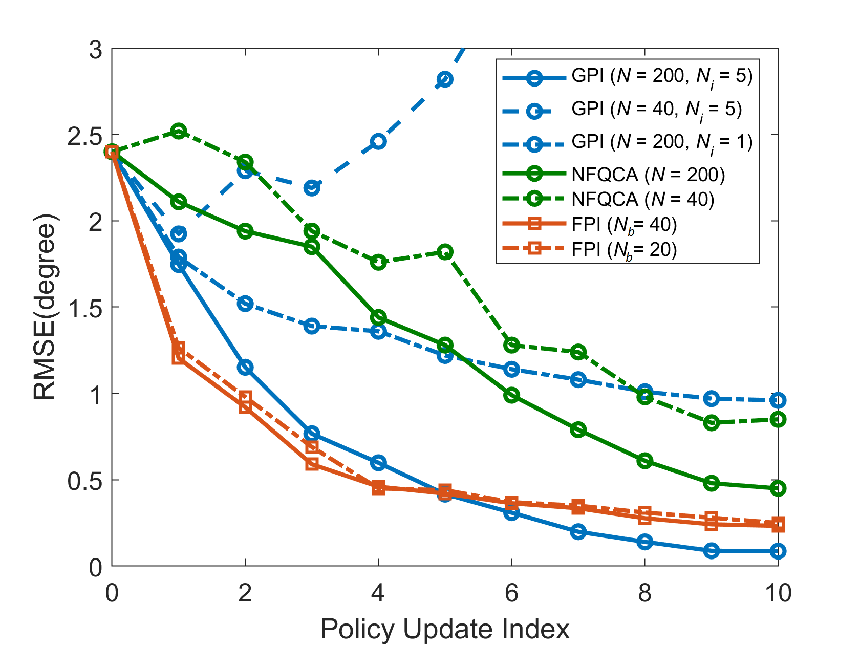
Figure 4: Comparison of the RMSEs between controlled knee profiles and target profiles using FPI, GPI and NFQCA under the same stage cost (52).

Table III shows a systematic comparison of the four algorithms under various noise conditions. Artificially generated noise and noise based on variations of human subject movement profiles were used in the comparisons. To be specific, sensor noise and actuator noise are uniform noise that are added to the states $x_{k}$ and actions $u_{k}$, respectively. In the last two rows, human variances collected from two amputee subjects TF1 and TF2 were introduced to the simulations, which would affect the states $x_{k}$. Under all noise conditions, FPI outperformed the other three existing algorithms in terms of both success rate and tuning time.

Fig. 4 compares the root-mean-square errors (RMSEs) between target knee angle profile and actual knee angle profile using FPI, GPI and NFQCA. Note that when we used a suggested parameter setting of ($N=40,N_{i}=5$) in GPI [69], the RMSE increased after a few iterations. Also note from Fig. 4 that, GPI may achieve a similar performance as the FPI but it required a much larger sample size of $N=200$ than FPI’s.

V-D FPI Incremental Mode Evaluation

We now evaluate FPI under incremental mode to further study FPI’s data and time efficiency. Both PER and learning from supplemental value, two of the innovative features of FPI, can be employed in this mode.

To obtain supplemental value $\mathcal{V}$ in (15) for the last row result in Table IV, we trained an FPI agent for just one trial in OpenSim under the same settings as those in the first row of Table (II) (Settings (A)(A)(A)(A) in Table I and $N_{b}=20$). Then supplemental value $\mathcal{V}$ is obtained from $(x_{k})=\underset{u_{k}}{\min}Q_{f}(x_{k},u_{k})$ where $Q_{f}(x_{k},u_{k})$ the final approximate value function after Algorithm 1 is terminated.

TABLE IV: FPI Tuner Performance under Incremental Mode

Configuration	Options*	Success Rate	Tuning Time (gait cycles)
ER	(A)(B)(A)(A)	83% (25/30)	134.4±21.6
PER	(A)(B)(B)(A)	83% (25/30)	127.6±25.8
PER+Supp value	(A)(B)(B)(B)	90% (27/30)	103.3±15.1

*refer to Table I. ER: Experience Replay; PER: Prioritized Experience Replay.

Table IV summarizes the performance of FPI in incremental mode under three different configurations. ER or PER reutilized past samples from the current trial for policy iteration (Settings 2(B) in Table I). The first configuration is the ER case without sample prioritization, i.e., $\lambda_{k}^{(i)}=1$ for all $k$. The second configurations prioritized the samples before performing the policy evaluation. In both the first and the second configurations (the first two rows in Table IV), no supplemental value was used, i.e., $\mathcal{V}(x_{k})=0$ for all $x_{k}.$ The third configuration (the third row in Table IV) utilized both prioritized samples and supplemental value. The supplemental value $\mathcal{V}(x_{k})$ was obtained from training FPI with a previous trial. In Table IV, the success rate increases from 83% to 90% as the algorithm gets more complex with PER and supplemental value. The results also suggest that the introduction of sample prioritization and supplemental value improves the data efficiency. Note that if the maximum number of gait cycles was extended from 500 to 1000, then the success rate of all simulation results in Table IV will be 100%.

A statistical summary of a 30 randomly initialized trials based on the condition in row 1 of Table IV is provided in Fig. 5 (bottom half panel). As shown, after tuning, the proposed FPI algorithm successfully reduced gait peak and duration errors.

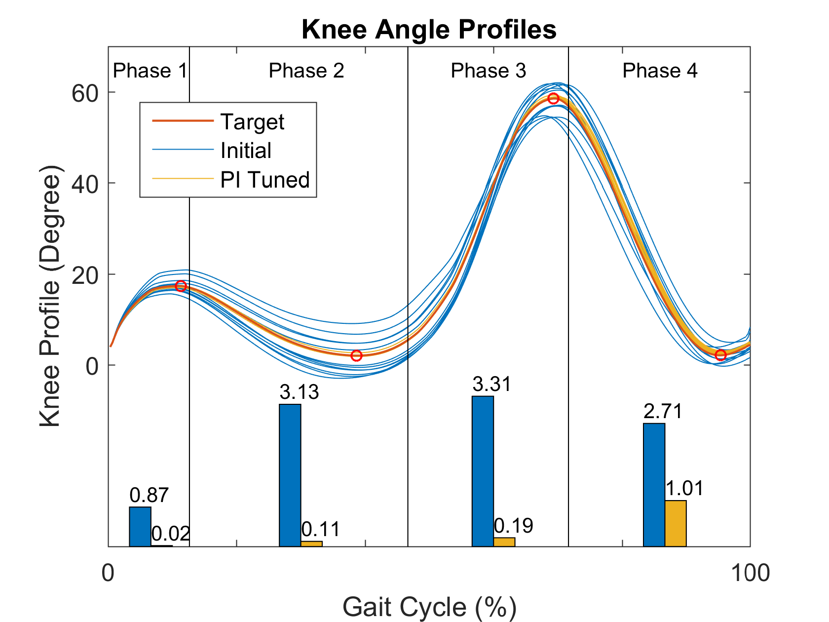
Figure 5: Before-and-after FPI tuning of knee profiles of 15 randomly selected trials. Top half: FPI enabled initial knee profiles (blue) approach the target knee profile (red), with FPI enabled, final knee profiles shown in yellow. Bottom half: The blue bars are the RMSEs between the initial knee angle profiles and the target knee profile, and the yellow bars are the RMSEs between the FPI tuned knee profiles and the target profile.

VI Conclusion

We have proposed a new flexible policy iteration (FPI) algorithm aimed at providing data and time efficient, high-dimensional control inputs to configure a robotic knee with human in the loop. The FPI incorporates previous samples and supplemental values during learning using prioritized experience replay and an augmented policy evaluation. Our results not only show qualitative properties of FPI as a stabilizing controller and that it approaches approximate (sub)optimal solution, but also include extensive simulation evaluations of control performance of FPI under different implementation conditions. We also compared FPI with other comparable algorithms, such as dHDP, NFQCA and GPI, which further demonstrates the efficacy of FPI as a data and time efficient learning controller. The FPI under batch mode became more efficient when utilizing (prioritized) experience replay and previous knowledge. Even though our application does not render itself as a big data problem, but our results show that FPI has the capability of efficiently working with a tight data budget. Specifically, FPI is capable of successfully tuning the control parameters within 100’s gait cycles under various conditions (Tables II and III), which is an equivalent of only a few minutes of walking time. Our results reported here represent the state of the art in automatic configuration of powered prosthetic knee devices. This result can potentially lead to practical use of the FPI in clinics. In turn, this can significantly reduce health care cost and improve the quality of life for the transfemoral amputee population in the world.

References

- [1] F. Sup et al., “Preliminary evaluations of a self-contained anthropomorphic transfemoral prosthesis,” IEEE/ASME Trans. Mechatronics, vol. 14, no. 6, pp. 667–676, Dec. 2009.
- [2] E. J. Rouse, L. M. Mooney, and H. M. Herr, “Clutchable series-elastic actuator: Implications for prosthetic knee design,” The International Journal of Robotics Research, vol. 33, no. 13, pp. 1611–1625, 2014.
- [3] A. M. Simon et al., “Configuring a powered knee and ankle prosthesis for transfemoral amputees within five specific ambulation modes,” PLoS One, vol. 9, no. 6, p. e99387, Jun. 2014.
- [4] R. D. Gregg, T. Lenzi, L. J. Hargrove, and J. W. Sensinger, “Virtual constraint control of a powered prosthetic leg: From simulation to experiments with transfemoral amputees,” IEEE Trans. Robot., vol. 30, no. 6, pp. 1455–1471, Dec. 2014.
- [5] H. Huang et al., “A cyber expert system for auto-tuning powered prosthesis impedance control parameters,” Ann. Biomed. Eng., vol. 44, no. 5, pp. 1613–1624, May 2016.
- [6] S. Pfeifer, H. Vallery, M. Hardegger, R. Riener, and E. J. Perreault, “Model-based estimation of knee stiffness,” IEEE Transactions on Biomedical Engineering, vol. 59, no. 9, pp. 2604–2612, 2012.
- [7] E. J. Rouse, L. J. Hargrove, E. J. Perreault, and T. a. Kuiken, “Estimation of human ankle impedance during the stance phase of walking,” IEEE Trans. Neural Syst. Rehabil. Eng., vol. 22, no. 4, pp. 870–878, Jul. 2014.
- [8] M. R. Tucker et al., “Design and characterization of an exoskeleton for perturbing the knee during gait,” IEEE Trans. Biomed. Eng., vol. 64, no. 10, pp. 2331–2343, Oct. 2017.
- [9] S. Kumar et al., “Extremum seeking control for model-free auto-tuning of powered prosthetic legs,” IEEE Transactions on Control Systems Technology, vol. 28, no. 6, pp. 2120–2135, 2020.
- [10] J. R. Koller et al., “’body-in-the-loop’ optimization of assistive robotic devices: A validation study,” in Proceedings of Robotics: Science and Systems, AnnArbor, Michigan, June 2016.
- [11] J. Zhang et al., “Human-in-the-loop optimization of exoskeleton assistance during walking,” Science, vol. 356, pp. 1280 – 1284, 2017.
- [12] Y. Ding, M. Kim, S. Kuindersma, and C. Walsh, “Human-in-the-loop optimization of hip assistance with a soft exosuit during walking,” Science Robotics, vol. 3, p. eaar5438, 02 2018.
- [13] N. Hogan, “Impedance control: An approach to manipulation: Applications,” J. Dyn. Syst. Meas. Control, vol. 107, no. 1, p. 17, Mar. 1985.
- [14] H. Geyer, A. Seyfarth, and R. Blickhan, “Positive force feedback in bouncing gaits?” Proceedings. Biological sciences / The Royal Society, vol. 270, pp. 2173–83, 11 2003.
- [15] K. Shamaei, G. S. Sawicki, and A. M. Dollar, “Estimation of quasi-stiffness of the human knee in the stance phase of walking,” PLOS ONE, vol. 8, no. 3, pp. 1–10, 03 2013.
- [16] M. Liu, F. Zhang, P. Datseris, and H. Huang, “Improving Finite State Impedance Control of Active-Transfemoral Prosthesis Using Dempster-Shafer Based State Transition Rules,” J. Intell. Robot. Syst. Theory Appl., vol. 76, no. 3-4, pp. 461–474, dec 2014.
- [17] S. Levine, C. Finn, T. Darrell, and P. Abbeel, “End-to-end training of deep visuomotor policies,” J. Mach. Learn. Res., vol. 17, no. 1, pp. 1334–1373, Jan. 2016.
- [18] V. Mnih et al., “Human-level control through deep reinforcement learning,” Nature, vol. 518, no. 7540, pp. 529–533, Feb. 2015.
- [19] D. Silver et al., “Mastering the game of go with deep neural networks and tree search,” Nature, vol. 529, no. 7587, pp. 484–489, 2016.
- [20] ——, “Mastering the game of go without human knowledge,” Nature, vol. 550, no. 7676, pp. 354–359, 2017.
- [21] F. Farahnakian, P. Liljeberg, and J. Plosila, “Energy-efficient virtual machines consolidation in cloud data centers using reinforcement learning,” in Euromicro Int. Conf. Parallel, Distrib. Network-Based Process. IEEE, Feb. 2014, pp. 500–507.
- [22] J. Si, A. G. Barto, W. B. Powell, and D. C. Wunsch, Handbook of learning and approximate dynamic programming. IEEE Press, 2004.
- [23] L. Frank and D. Liu, Eds., Reinforcement learning and approximate dynamic programming for feedback control. Piscataway, NJ: John Wiley & Sons, 2012.
- [24] C. Lu, J. Si, and X. Xie, “Direct heuristic dynamic programming for damping oscillations in a large power system,” IEEE Trans. Syst. Man, Cybern. Part B Cybern., vol. 38, no. 4, pp. 1008–1013, Aug. 2008.
- [25] W. Guo, F. Liu, J. Si, D. He, R. Harley, and S. Mei, “Approximate dynamic programming based supplementary reactive power control for dfig wind farm to enhance power system stability,” Neurocomputing, vol. 170, pp. 417–427, Dec. 2015.
- [26] ——, “Online supplementary adp learning controller design and application to power system frequency control with large-scale wind energy integration,” IEEE Trans. Neural Networks Learn. Syst., vol. 27, no. 8, pp. 1748–1761, 2016.
- [27] R. Enns and J. Si, “Apache helicopter stabilization using neural dynamic programming,” J. Guid. Control. Dyn., vol. 25, no. 1, pp. 19–25, Jan. 2002.
- [28] ——, “Helicopter trimming and tracking control using direct neural dynamic programming,” IEEE Trans. Neural Networks, vol. 14, no. 4, pp. 929–939, Jul. 2003.
- [29] Y. Wen, M. Liu, J. Si, and H. Huang, “Adaptive control of powered transfemoral prostheses based on adaptive dynamic programming,” Proc. Annu. Int. Conf. IEEE EMBS, pp. 5071–5074, 2016.
- [30] Y. Wen, J. Si, X. Gao, S. Huang, and H. Huang, “A New Powered Lower Limb Prosthesis Control Framework Based on Adaptive Dynamic Programming,” IEEE Trans. Neural Networks Learn. Syst., vol. 28, no. 9, pp. 2215–2220, sep 2017.
- [31] Y. Wen, J. Si, A. Brandt, X. Gao, and H. Huang, “Online Reinforcement Learning Control for the Personalization of a Robotic Knee Prosthesis,” IEEE Trans. Cybern., pp. 1–11, jan 2019.
- [32] J. Si and Y. T. Wang, “On-line learning control by association and reinforcement,” IEEE Trans. Neural Networks, vol. 12, no. 2, pp. 264–76, mar 2001.
- [33] M. G. Lagoudakis and R. Parr, “Least-squares policy iteration,” J. Mach. Learn. Res., vol. 4, no. 6, pp. 1107–1149, Dec. 2003.
- [34] F. Liu, J. Sun, J. Si, W. Guo, and S. Mei, “A boundedness result for the direct heuristic dynamic programming,” Neural Networks, vol. 32, pp. 229–235, Aug. 2012.
- [35] W. Gao and Z. Jiang, “Learning-based adaptive optimal tracking control of strict-feedback nonlinear systems,” IEEE Transactions on Neural Networks and Learning Systems, vol. 29, no. 6, pp. 2614–2624, 2018.
- [36] Y. Jiang and Z. Jiang, “Global adaptive dynamic programming for continuous-time nonlinear systems,” IEEE Transactions on Automatic Control, vol. 60, no. 11, pp. 2917–2929, 2015.
- [37] T. Bian, Y. Jiang, and Z. Jiang, “Adaptive dynamic programming and optimal control of nonlinear nonaffine systems,” Automatica, vol. 50, no. 10, pp. 2624 – 2632, 2014.
- [38] Y. Jiang, J. Fan, T. Chai, and F. L. Lewis, “Dual-rate operational optimal control for flotation industrial process with unknown operational model,” IEEE Trans. Ind. Elects., vol. 66, no. 6, pp. 4587–4599, 2019.
- [39] A. Al-Tamimi, F. L. Lewis, and M. Abu-Khalaf, “Discrete-time nonlinear HJB solution using approximate dynamic programming: Convergence proof,” IEEE Trans. Syst. Man, Cybern. Part B Cybern., vol. 38, no. 4, pp. 943–949, jun 2008.
- [40] C. Mu, D. Wang, and H. He, “Novel iterative neural dynamic programming for data-based approximate optimal control design,” Automatica, vol. 81, pp. 240 – 252, 2017.
- [41] D. Liu and Q. Wei, “Policy iteration adaptive dynamic programming algorithm for discrete-time nonlinear systems,” IEEE Trans. Neural Networks Learn. Syst., vol. 25, no. 3, pp. 621–634, Mar. 2014.
- [42] Q. Wei and D. Liu, “A novel policy iteration based deterministic q-learning for discrete-time nonlinear systems,” Sci. China Inf. Sci., vol. 58, no. 12, pp. 1–15, Dec. 2015.
- [43] Q. Wei, D. Liu, Q. Lin, and R. Song, “Discrete-time optimal control via local policy iteration adaptive dynamic programming,” IEEE Trans. Cybern., vol. 47, no. 10, pp. 3367–3379, Oct. 2017.
- [44] W. Guo, J. Si, F. Liu, and S. Mei, “Policy approximation in policy iteration approximate dynamic programming for discrete-time nonlinear systems,” IEEE Trans. Neural Networks Learn. Syst., vol. 29, no. 7, pp. 2794 – 2807, Jul. 2018.
- [45] L. J. Lin, “Self-improving reactive agents based on reinforcement learning, planning and teaching,” Mach. Learn., vol. 8, no. 3, pp. 293–321, 1992.
- [46] D. Isele and A. Cosgun, “Selective experience replay for lifelong learning,” in AAAI Conf. Artif. Intell., 2018, pp. 3302–3309.
- [47] T. Schaul, J. Quan, I. Antonoglou, and D. Silver, “Prioritized experience replay,” in Proc. Int. Conf. Learn. Represent., Nov. 2015.
- [48] D. Horgan et al., “Distributed prioritized experience replay,” in Int. Conf. Learn. Represent., Mar. 2018.
- [49] M. Andrychowicz et al., “Hindsight experience replay,” in Adv. Neural Inf. Process. Syst., 2017.
- [50] S. Adam, L. Busoniu, and R. Babuska, “Experience replay for real-time reinforcement learning control,” IEEE Trans. Syst. Man Cybern. Part C Appl. Rev., vol. 42, no. 2, pp. 201–212, Mar. 2012.
- [51] B. Luo, Y. Yang, and D. Liu, “Adaptive q-learning for data-based optimal output regulation with experience replay,” IEEE Trans. Cybern., vol. 48, no. 12, pp. 3337–3348, Mar. 2018.
- [52] G. Chowdhary et al., “Concurrent learning adaptive control of linear systems with exponentially convergent bounds,” Int. J. Adapt. Ctrl and Sig. Proc., vol. 27, no. 4, pp. 280–301, 2013.
- [53] H. Modares, F. L. Lewis, and M. B. Naghibi-Sistani, “Integral reinforcement learning and experience replay for adaptive optimal control of partially-unknown constrained-input continuous-time systems,” Automatica, vol. 50, pp. 193–202, 2014.
- [54] K. G. Vamvoudakis, M. F. Miranda, and J. P. Hespanha, “Asymptotically stable adaptive optimal control algorithm with saturating actuators and relaxed persistence of excitation,” IEEE Transactions on Neural Networks, vol. 27, no. 11, pp. 2386–2398, 2016.
- [55] D. Zhao, Q. Zhang, D. Wang, and Y. Zhu, “Experience Replay for Optimal Control of Nonzero-Sum Game Systems with Unknown Dynamics,” IEEE Trans. Cybern., vol. 46, no. 3, pp. 854–865, mar 2016.
- [56] X. Yang and H. He, “Adaptive critic learning and experience replay for decentralized event-triggered control of nonlinear interconnected systems,” IEEE Trans. Syst. Man, Cybern. Syst., pp. 1–13, 2019.
- [57] M. E. Taylor and P. Stone, “Transfer Learning for Reinforcement Learning Domains : A Survey,” J. Mach. Learn. Res., vol. 10, pp. 1633–1685, 2009.
- [58] D. Abel et al., “Policy and Value Transfer in Lifelong Reinforcement Learning,” in Int. Conf. Mach. Learn., 2018, pp. 20–29.
- [59] A. Lazaric, “Transfer in reinforcement learning: A framework and a survey,” in Reinf. Learn. Adapt. Learn. Optim., Wiering M. and v. O. M., Eds. Springer, 2012, ch. 12, pp. 143–173.
- [60] M. E. Taylor and P. Stone, “Behavior transfer for value-function-based reinforcement learning,” in Proc. Int. Conf. Auton. Agents, 2005.
- [61] F. Fernández and M. Veloso, “Probabilistic policy reuse in a reinforcement learning agent,” in Proc. Int. Conf. Auton. Agents, 2006.
- [62] S. Griffith et al., “Policy shaping: Integrating human feedback with Reinforcement Learning,” in Adv. Neural Inf. Process. Syst., 2013.
- [63] G. Konidaris and A. Barto, “Autonomous shaping: knowledge transfer in reinforcement learning,” in Proc. 23rd Int. Conf. Mach. Learn. - ICML ’06. New York, New York, USA: ACM Press, 2006, pp. 489–496.
- [64] A. Y. Ng, D. Harada, and S. Russell, “Policy invariance under reward transformations : Theory and application to reward shaping,” in Int. Conf. Mach. Learn., 1999, pp. 278–287.
- [65] T. Mann et al., “Directed exploration in reinforcement learning with transferred knowledge,” Journal of Machine Learning Research: Workshop & Conference Proceedings, vol. 24, pp. 59–75, 01 2012.
- [66] Y. Wen, A. Brandt, M. Liu, H. Helen, and J. Si, “Comparing parallel and sequential control parameter tuning for a powered knee prosthesis,” in IEEE Int., Conf. Sys., Man Cybern., 2017, pp. 1716–1721.
- [67] E. C. Martinez-villalpando and H. Herr, “Agonist-antagonist active knee prosthesis: A preliminary study in level-ground walking,” J. Rehabil. Res. Dev., vol. 46, no. 3, pp. 361–373, Feb. 2009.
- [68] A. Brandt, Y. Wen, M. Liu, J. Stallings, and H. Huang, “Interactions between transfemoral amputees and a powered knee prosthesis during load carriage,” Sci. Rep., vol. 7, no. 1, Nov. 2017.
- [69] D. Liu, Q. Wei, and P. Yan, “Generalized policy iteration adaptive dynamic programming for discrete-time nonlinear systems,” IEEE Trans. Syst. Man, Cybern. Syst., vol. 45, no. 12, pp. 1577–1591, May 2015.
- [70] R. Hafner and M. Riedmiller, “Reinforcement learning in feedback control : Challenges and benchmarks from technical process control,” Mach. Learn., vol. 84, no. 1-2, pp. 137–169, Jul. 2011.