Provable Training Set Debugging for Linear Regression

Abstract

We investigate problems in penalized $M$-estimation, inspired by applications in machine learning debugging. Data are collected from two pools, one containing data with possibly contaminated labels, and the other which is known to contain only cleanly labeled points. We first formulate a general statistical algorithm for identifying buggy points and provide rigorous theoretical guarantees when the data follow a linear model. We then propose an algorithm for tuning parameter selection of our Lasso-based algorithm with theoretical guarantees. Finally, we consider a two-person “game" played between a bug generator and a debugger, where the debugger can augment the contaminated data set with cleanly labeled versions of points in the original data pool. We develop and analyze a debugging strategy in terms of a Mixed Integer Linear Programming (MILP). Finally, we provide empirical results to verify our theoretical results and the utility of the MILP strategy.

Keywords Robust Statistics  $\cdot$ Outlier Detection  $\cdot$ Tuning Parameter Selection  $\cdot$ Optimization

1 Introduction

Modern machine learning systems are extremely sensitive to training set contamination. Since sources of error and noise are unavoidable in real-world data (e.g., due to Mechanical Turkers, selection bias, or adversarial attacks), an urgent need has arisen to perform automatic debugging of large data sets. Cadamuro et al. [cadamuro2016debugging] and Zhang et al. [zhang2018training] proposed a method called “machine learning debugging” to identify training set errors by introducing new clean data. Consider the following real-world scenario: Company A collects movie ratings for users on a media platform, from which it learns relationships between features of movies and ratings in order to perform future recommendations. A competing company B knows A’s learning method and hires some users to provide malicious ratings. Company A could employ a robust method for learning contaminated data—but in the long run, it would be more effective for company A to identify the adversarial users and prevent them from submitting additional buggy ratings in the future. This distinguishes debugging from classical learning. The debugging problem also assumes that company A can hire an expert to help rate movies, from which it obtains a second trusted data set which is generally smaller than the original data set due to budget limitations. In this paper, we will study a theoretical framework for the machine learning debugging problem in a linear regression setting, where the main goal is to identify bugs in the data. We will also discuss theory and algorithms for selecting the trusted data set.

Our first contribution is to provide a rigorous theoretical framework explaining how to identify errors in the “buggy" data pool. Specifically, we embed a squared loss term applied to the trusted data pool into the extended Lasso algorithm proposed by Nguyen and Tran [nguyen2013robust], and reformulate the objective to better service the debugging task. Borrowing techniques from robust statistics [huber2009robust, she2011outlier, nguyen2013robust, foygel2014corrupted, slawski2017linear] and leveraging results on support recovery analysis [wainwright2009sharp, meinshausen2009lasso], we provide sufficient conditions for successful debugging in linear regression. We emphasize that our setting, involving data coming from multiple pools, has not been studied in any of the earlier papers.

The work of Nguyen and Tran [nguyen2013robust] and Foygel and Mackey [foygel2014corrupted] (and more recently, Sasai and Fujisawa [sasai2020robust]) provided results for the extended Lasso with a theoretically optimal choice of tuning parameter, which depends on the unknown noise variance in the linear model. Our second contribution is to discuss a rigorous procedure for tuning parameter selection which does not require such an assumption. Specifically, our algorithm starts from a sufficiently large initial tuning parameter that produces the all-zeros vector as an estimator. Assuming the sufficient conditions for successful support recovery are met, this tuning parameter selection algorithm is guaranteed to terminate with a correct choice of tuning parameter after a logarithmic number of steps. Note that when outliers exist in the training data set, it is improper to use cross-validation to select the tuning parameter due to possible outliers in the validation data set.

Our third contribution considers how to design a second clean data pool, which is an important but previously unstudied problem in machine learning debugging. We consider a two-player “game" between a bug generator and debugger, where the bug generator performs adversarial attacks [chakraborty2018adversarial], and the debugger applies Lasso-based linear regression to the augmented data set. On the theoretical side, we establish a sufficient condition under which the debugger can always beat the bug generator, and show how to translate this condition into a debugging strategy based on mixed integer linear programming. Our theory is only derived in the “noiseless” setting; nonetheless, empirical simulations show that our debugging strategy also performs well in the noisy setting. We experimentally compare our method to two other algorithms motivated by the machine learning literature, which involve designing two neural networks, one to correct labels and one to fit cleaned data [veit2017learning]; and a method based on semi-supervised learning that weights the noisy and clean datasets differently and employs a similarity matrix based on the graph Laplacian [fergus2009semi].

The remainder of the paper is organized as follows: Section 2 introduces our novel framework for machine learning debugging using weighted $M$-estimators. Section 3 provides theoretical guarantees for recovery of buggy data points. Section 4 presents our algorithm for tuning parameter selection and corresponding theoretical guarantees. Section 5 discusses strategies for designing the second pool. Section 6 provides experimental results. Section 7 concludes the paper.

Notation: We write $\Lambda_{\min}(A)$ and $\Lambda_{\max}(A)$ to denote the minimum and maximum eigenvalues, respectively, of a matrix $A$. We use $Null(A)$ to denote the nullspace of $A$. For subsets of row and column indices $S$ and $T$, we write $A_{S,T}$ to denote the corresponding submatrix of $A$. We write $\|A\|_{\max}$ to denote the elementwise $\ell_{\infty}$-norm, $\|A\|_{2}$ to denote the spectral norm, and $\|A\|_{\infty}$ to denote the $\ell_{\infty}$-operator norm. For a vector $v\in{}^{n}$, we write $\operatorname{supp}(v)\subseteq\{1,\dots,n\}$ to denote the support of $v$, and $\|v\|_{\infty}=\max|v_{i}|$ to denote the maximum absolute entry. We write $\|v\|_{p}$ to denote the $\ell_{p}$-norm, for $p\geq 1$. We write $\operatorname{diag}(v)$ to denote the $n\times n$ diagonal matrix with entries equal to the components of $v$. For $S\subseteq\{1,\dots,n\}$, we write $v_{S}$ to denote the $|S|$-dimensional vector obtained by restricting $v$ to $S$. We write $[n]$ as shorthand for $\{1,\dots,n\}$.

2 PROBLEM FORMULATION

We first formalize the data-generating models analyzed in this paper. Suppose we have observation pairs $\{(x_{i},y_{i})\}_{i=1}^{n}$ from the contaminated linear model

$$y_{i}=x_{i}^{\top}\beta^{*}+\gamma^{*}_{i}+\epsilon_{i},\qquad 1\leq i\leq n,$$ (1)

where $\beta^{*}\in{}^{p}$ is the unknown regression vector, $\gamma^{*}\in{}^{n}$ represents possible contamination in the labels, and the $\epsilon_{i}$’s are i.i.d. sub-Gaussian noise variables with variance parameter $\sigma^{2}$. We also assume the $x_{i}$’s are i.i.d. and $x_{i}\perp\!\!\!\perp\epsilon_{i}$. This constitutes the “first pool." Note that the vector $\gamma^{*}$ is unknown and may be generated by some adversary. If $\gamma^{*}_{i}=0$, the $i^{\text{th}}$ point is uncontaminated and follows the usual linear model; if $\gamma^{*}_{i}\neq 0$, the $i^{\text{th}}$ point is contaminated/buggy. Let $T:=\operatorname{supp}(\gamma^{*})$ denote the indices of the buggy points, and let $t:=|T|$ denote the number of bugs.

We also assume we have a clean data set which we call the “second pool." We observe $\{(\widetilde{x}_{i},\widetilde{y}_{i})\}_{i=1}^{m}$ satisfying

$$\widetilde{y}_{i}=\widetilde{x}_{i}^{\top}\beta^{*}+\widetilde{\epsilon}_{i},\qquad 1\leq i\leq m,$$ (2)

where the $\widetilde{\epsilon}_{i}$’s are i.i.d. sub-Gaussian noise variables with parameter $\widetilde{\sigma}^{2}$. Let $L:=\frac{\sigma}{\widetilde{\sigma}}$, and suppose $L\geq 1$. Unlike the first pool, the data points in the second pool are all known to be uncontaminated.

For notational convenience, we also use $X\in{}^{n\times p}$, $y\in{}^{n}$, and $\epsilon\in{}^{m}$ to denote the matrix/vectors containing the $x_{i}$’s, $y_{i}$’s, and $\epsilon_{i}$’s, respectively. Similarly, we define the matrices $\widetilde{X}\in{}^{m\times p},\widetilde{y}\in{}^{m}$, and $\widetilde{\epsilon}\in{}^{m}$. Note that $\beta^{*},\gamma^{*},T,t$, and the noise parameters $\sigma$ and $\widetilde{\sigma}$ are all assumed to be unknown to the debugger. In this paper, we will work in settings where $X^{\top}X$ is invertible.

Goal:

Upon observing $\{(x_{i},y_{i})\}_{i=1}^{n}$, the debugger is allowed to design $m$ points $\widetilde{X}$ in a stochastic or deterministic manner and query their corresponding labels $\widetilde{y}$, with the goal of recovering the support of $\gamma^{*}$. We have the following definitions:

Definition 1.

An estimator $\widehat{\gamma}$ satisfies subset support recovery if $\operatorname{supp}(\widehat{\gamma})\subseteq\operatorname{supp}(\gamma^{*})$. It satisfies exact support recovery if $\operatorname{supp}(\widehat{\gamma})=\operatorname{supp}(\gamma^{*})$.

In words, when $\widehat{\gamma}$ satisfies subset support recovery, all estimated bugs are true bugs. When $\widehat{\gamma}$ satisfies exact support recovery, the debugger correctly flags all bugs. We are primarily interested in exact support recovery.

Weighted $M$-estimation Algorithm: We propose to optimize the joint objective

$$\begin{split}(\widehat{\beta},\widehat{\gamma})\in&\arg\min_{\beta\in{}^{p},\gamma\in{}^{n}}\left\{\frac{1}{2n}\|y-X\beta-\gamma\|_{2}^{2}+\frac{\eta}{2m}\|\widetilde{y}-\widetilde{X}\beta\|_{2}^{2}+\lambda\|\gamma\|_{1}\right\},\end{split}$$ (3)

where the weight parameter $\eta>0$ determines the relative importance of the two data pools. The objective function applies the usual squared loss to the points in the second pool and introduces the additional variable $\gamma$ to help identify bugs in the first pool. Furthermore, the $\ell_{1}$-penalty encourages $\widehat{\gamma}$ to be sparse, since we are working in settings where the number of outliers is relatively small compared to the total number of data points. Note that the objective function (3) may equivalently be formulated as a weighted sum of $M$-estimators applied to the first and second pools, where the loss for the first pool is the robust Huber loss and the loss for the second pool is the squared loss (cf. Proposition LABEL:PropWeightedM in Appendix LABEL:sec:app-additional-discussion).

Lasso Reformulation: Recall that our main goal is to estimate (the support of) $\gamma^{*}$ rather than $\beta^{*}$. Thus, we will restrict our attention to $\gamma^{*}$ by reformulating the objectives appropriately. We first introduce some notation: Define the stacked vectors/matrices

$$X^{\prime}=\begin{pmatrix}X\\ \sqrt{\frac{\eta n}{m}}\widetilde{X}\end{pmatrix},y^{\prime}=\begin{pmatrix}y\\ \sqrt{\frac{\eta n}{m}}\widetilde{y}\end{pmatrix},\epsilon^{\prime}=\begin{pmatrix}\epsilon\\ \sqrt{\frac{\eta n}{m}}\tilde{\epsilon}\end{pmatrix},$$ (4)

where $X^{\prime}\in{}^{(m+n)\times p}$ and $y^{\prime},\epsilon^{\prime}\in{}^{m+n}$. For a matrix $A$, let $P_{A}=A(A^{\top}A)^{-1}A^{\top}$ and $P_{A}^{\perp}=I-A(A^{\top}A)^{-1}A^{\top}$ denote projection matrices onto the range of the column space of $A$ and its orthogonal complement, respectively. For a matrix $S\subseteq[n]$, let $M_{S}$ denote the $(n+m)\times|S|$ matrix with $i^{\text{th}}$ column equal to the canonical vector $e_{S(i)}$. Thus, right-multiplying by $M_{S}$ truncates a matrix to only include columns indexed by $S$. We have the following useful result:

Proposition 1.

The objective function

$$\widehat{\gamma}\in\arg\min_{\gamma\in{}^{n}}\Big{\{}\frac{1}{2n}\|P_{X^{\prime}}^{\perp}y^{\prime}-P_{X^{\prime}}^{\perp}M_{[n]}\gamma\|_{2}^{2}+\lambda\|\gamma\|_{1}\Big{\}}$$ (5)

shares the same solution for $\widehat{\gamma}$ with the objective function (3).

Proposition 1, proved in Appendix LABEL:AppSecFormu, translates the joint optimization problem (3) into an optimization problem only involving the parameter of interest $\gamma$. We provide a discussion regarding the corresponding solution $\widehat{\beta}$ in Appendix LABEL:sec:app-additional-discussion for the interested reader. Note that the optimization problem (5) corresponds to linear regression of the vector/matrix pairs $(P_{X^{\prime}}^{\perp}y^{\prime},P_{X^{\prime}}^{\perp}M_{[n]})$ with a Lasso penalty, inspiring us to borrow techniques from high-dimensional statistics.

3 SUPPORT RECOVERY

The reformulation (5) allows us to analyze the machine learning debugging framework through the lens of Lasso support recovery. The three key conditions we impose to ensure support recovery are provided below. Recall that we use $M_{T}$ to represent the truncation matrix indexed by $T$.

Assumption 1 (Minimum Eigenvalue).

Assume that there is a positive number $b^{\prime}_{\min}$ such that

$$\Lambda_{\min}\left(M_{T}^{\top}P_{X^{\prime}}^{\perp}M_{T}\right)\geq b^{\prime}_{\min}.$$ (6)

Assumption 2 (Mutual Incoherence).

Assume that there is a number $\alpha^{\prime}\in[0,1)$ such that

$$\|M_{T^{c}}^{\top}P_{X^{\prime}}^{\perp}M_{T}(M_{T}^{\top}P_{X^{\prime}}^{\perp}M_{T})^{-1}\|_{\infty}\leq\alpha^{\prime}.$$ (7)

Assumption 3 (Gamma-Min).

Assume that

$$\begin{split}\min_{i\in T}|\gamma^{*}_{i}|>G^{\prime}&:=\|(M_{T}^{\top}P_{X^{\prime}}^{\perp}M_{T})^{-1}M_{T}^{\top}P_{X^{\prime}}^{\perp}\epsilon^{\prime}\|_{\infty}+n\lambda\left|\!\left|\!\left|{(M_{T}^{\top}P_{X^{\prime}}^{\perp}M_{T})^{-1}}\right|\!\right|\!\right|_{\infty}.\end{split}$$ (8)

Assumption 1 comes from a primal-dual witness argument [wainwright2009sharp] to guarantee that the minimizer $\widehat{\gamma}$ is unique. Assumption 2 measures a relationship between the sets $T^{c}$ and $T$, indicating that the large number of nonbuggy covariates (i.e., $T^{c}$) cannot exert an overly strong effect on the subset of buggy covariates [ravikumar2010high]. To aid intuition, consider an orthogonal design, where $X=\begin{bmatrix}cI_{[t],[p]}\\ c^{\prime}I_{p\times p}\end{bmatrix}$ and $\widetilde{X}=c^{\prime\prime}I_{p\times p}$, for some $t<p$, and $c,c^{\prime},c^{\prime\prime}>0$. We use the notation $I_{[t],[p]}$ to denote a submatrix of $I_{p\times p}$ with rows indexed by the set $[t]$. Suppose the first $t$ points are bugs, and for simplicity, let $\eta=m/n$. Then the mutual incoherence condition requires $c<c^{\prime}+\frac{(c^{\prime\prime})^{2}}{c^{\prime}}$, meaning that in every direction $e_{i}$, the component of buggy data cannot be too large compared to the nonbuggy data and the clean data. Assumption 3 lower-bounds the minimum absolute value of elements of $\gamma$. Note that $\lambda$ is chosen based on $\epsilon^{\prime}$, so the right-hand expression is a function of $\epsilon^{\prime}$. This assumption indeed captures the intuition that the signal-to-noise ratio, $\frac{\min_{i\in T}{|\gamma^{*}_{i}|}}{\sigma}$, needs to be sufficiently large.

We now provide two general theorems regarding subset support recovery and exact support recovery.

Theorem 2 (Subset support recovery).

Suppose $P_{X^{\prime}}^{\perp}$ satisfies Assumptions 1 and 2. If the tuning parameter satisfies

$$\begin{split}\lambda&\geq\frac{2}{1-\alpha^{\prime}}\Big{\|}M_{T^{c}}P_{X^{\prime}}^{\perp}\Big{(}I-P_{X^{\prime}}^{\perp}M_{T}(M_{T}^{\top}P_{X^{\prime}}^{\perp}M_{T})^{-1}M_{T}^{\top}P_{X^{\prime}}^{\perp}\Big{)}\frac{\epsilon^{\prime}}{n}\Big{\|}_{\infty},\end{split}$$ (9)

then the objective (5) has a unique optimal solution $\widehat{\gamma}$, satisfying $\operatorname{supp}(\widehat{\gamma})\subseteq\operatorname{supp}(\gamma^{*})$ and $\left\lVert\widehat{\gamma}-\gamma^{*}\right\rVert_{\infty}\leq G^{\prime}$.

Theorem 3 (Exact support recovery).

In addition to the assumptions in Theorem 2, suppose Assumption 3 holds. Then we have a unique optimal solution $\widehat{\gamma}$, which satisfies exact support recovery.

Note that we additionally need Assumption 3 to guarantee exact support recovery. This follows the aforementioned intuition regarding the assumption. In particular, recall that $\epsilon$ and $\widetilde{\epsilon}$ are sub-Gaussian vectors with parameters $\sigma^{2}$ and $\sigma^{2}/L$, respectively, where $L\geq 1$ (i.e., the clean data pool has smaller noise). The minimum signal strength $\min_{i\in T}{|\gamma^{*}_{i}|}$ needs to be at least $\Theta(\sigma\sqrt{\log n})$, since $\mathbb{E}\left[\max_{i\in[n]}|\epsilon_{i}|\right]\leq\sigma\sqrt{2\log(2n)}$. Intuitively, if $\min_{i\in T}{|\gamma^{*}_{i}|}$ is of constant order, it is difficult for the debugger to distinguish between random noise and intentional contamination.

We now present two special cases to illustrate the theoretical benefits of including a second data pool. Although Theorems 2 and 3 are stated in terms of deterministic design matrices and error vectors $\epsilon$ and $\widetilde{\epsilon}$, the assumptions can be shown to hold with high probability in the example. We provide formal statements of the associated results in Appendix LABEL:app:ortho-design and Appendix LABEL:app:subgaussian-design.

Example 4 (Orthogonal design).

Suppose $Q$ is an orthogonal matrix with columns $q_{1},q_{2},\dots,q_{p}$, and consider the setting where $X_{T}=RQ^{\top}\in{}^{t\times p}$ and $X_{T^{c}}=FQ^{\top}\in{}^{p\times p}$, where $R=\left[\operatorname{diag}(\{r_{i}\}_{i=1}^{t})\mid\bm{0}_{t\times(p-t)}\right]$ and $F=\operatorname{diag}(\{f_{i}\}_{i=1}^{p})$. Thus, points in the contaminated first pool correspond to orthogonal vectors. Similarly, suppose the second pool consists of (rescaled) columns of $Q$, so $\widetilde{X}=WQ^{\top}\in{}^{m\times p}$, where $W=\operatorname{diag}(\{w_{i}\}_{i=1}^{p})$. (To visualize this setting, one can consider $Q=I$ as a special case.) The mutual incoherence parameter is $\alpha^{\prime}=\max_{1\leq i\leq t}\left|\frac{r_{i}f_{i}}{f_{i}^{2}+\eta\frac{n}{m}w_{i}^{2}}\right|$. Hence, $\alpha^{\prime}<1$ if the weight of a contaminated point dominates the weight of a clean point in any direction, e.g., when $|r_{i}|>|f_{i}|$ and $w_{i}=0$; in contrast, if the second pool includes clean points $w_{i}q_{i}$ with sufficiently large $|w_{i}|$, we can guarantee that $\alpha^{\prime}<1$. Furthermore,

$$G^{\prime}\approx\sigma\left(\sqrt{2\log t}+c\right)\sqrt{1+\max_{1\leq i\leq t}\frac{r_{i}^{2}(Lf_{i}^{2}+\frac{\eta n}{m}w_{i}^{2})}{L(f_{i}^{2}+\frac{\eta n}{m}w_{i}^{2})^{2}}}+\frac{2\sigma}{1-\alpha^{\prime}}\left(\sqrt{\log 2(n-t)}+C\right)\left(1+\max_{1\leq i\leq t}\frac{r_{i}^{2}}{f_{i}^{2}+\frac{\eta n}{m}w_{i}^{2}}\right)$$

for some constant $C$. It is not hard to verify that $G^{\prime}$ decreases by adding a second pool. Further note that the behavior of the non-buggy subspace, $\mathrm{span}\{q_{t+1},\dots,q_{p}\}$, is not involved in any conditions or conclusions. Thus, our key observation is that the theoretical results for support recovery consistency only rely on the addition of second-pool points in buggy directions.

Example 5 (Random design).

Consider a random design setting where the rows of $X$ and $\widetilde{X}$ are drawn from a common sub-Gaussian distribution with covariance $\Sigma$. The conditions in Assumptions 1–3 are relaxed in the presence of a second data pool when $n$ and $m$ are large compared to $p$: First, $b_{\min}^{\prime}$ increases by adding a second pool. Second, $\alpha^{\prime}\approx\frac{\|X_{T^{c}}\Sigma^{-1}X_{T}\|_{\infty}}{n-t+\eta n}$, so the mutual incoherence parameter also decreases by adding a second pool. Third,

$$G^{\prime}\approx\frac{2\sigma\sqrt{\log t}}{b^{\prime}_{\min}}+\frac{2\sigma}{1-\alpha^{\prime}}\max\left\{1,\sqrt{\frac{\eta n}{mL}}\right\}\left\|(I_{t\times t}-\frac{X_{T}\Sigma^{-1}X_{T}^{\top}}{n+\eta n})^{-1}\right\|_{\infty},$$

where $X_{T}$ and $X_{T^{c}}$ represent the submatrices of $X$ with rows indexed by $T$ and $T^{c}$, respectively. Note that the one-pool case corresponds to $\eta=0$ and $\left\|(I_{t\times t}-\frac{X_{T}\Sigma^{-1}X_{T}^{\top}}{n+\eta n})^{-1}\right\|_{\infty}<\left\|(I_{t\times t}-\frac{X_{T}\Sigma^{-1}X_{T}^{\top}}{n})^{-1}\right\|_{\infty}$, so if we choose $\eta\leq\frac{mL}{n}$, then $G^{\prime}$ decreases by adding a second pool. Therefore, all three assumptions are relaxed by having a second pool, making it easier to achieve exact support recovery.

We also briefly discuss the three assumptions with respect to the weight parameter $\eta$: Increasing $\eta$ always relaxes the eigenvalue and mutual incoherence conditions, so placing more weight on the second pool generally helps with subset support recovery. However, the same trend does not necessarily hold for exact recovery. This is because a larger value of $\eta$ causes the lower bound (9) on $\lambda$ to increase, resulting in a stricter gamma-min condition. Therefore, there is a tradeoff for selecting $\eta$.

4 TUNING PARAMETER SELECTION

A drawback of the results in the previous section is that the proper choice of tuning parameter depends on a lower bound (9) which cannot be calculated without knowledge of the unknown parameters $(T,\alpha^{\prime},\epsilon^{\prime})$. The tuning parameter $\lambda$ determines how many outliers a debugger detects; if $\lambda$ is large, then $\widehat{\gamma}$ contains more zeros and the algorithm detects fewer bugs. A natural question arises: In settings where the conditions for exact support recovery hold, can we select a data-dependent tuning parameter that correctly identifies all bugs? In this section, we propose an algorithm which answers this question in the affirmative.

4.1 Algorithm and Theoretical Guarantees

Our tuning parameter selection algorithm is summarized in Algorithm 1, which searches through a range of parameter values for $\lambda$, starting from a large value $\lambda_{u}$ and then halving the parameter on each successive step until a stopping criterion is met. The intuition is as follows: First, let $\lambda^{*}$ be the right-hand expression of inequality (9). Suppose that for any value in $I=[\lambda^{*},2\lambda^{*}]$, support recovery holds. Then given $\lambda_{u}>\lambda^{*}$, the geometric series $\Lambda=\left\{\lambda_{u},\frac{\lambda_{u}}{2},\frac{\lambda_{u}}{4},\dots\right\}$ must contain at least one correct parameter for exact support recovery since $\Lambda\cap I\neq\emptyset$, guaranteeing that the algorithm stops. As for the stopping criterion, let $X_{S}$ denote the submatrix of $X$ with rows indexed by $S$ for $T^{c}\subseteq S\subseteq[n]$. We have $P_{X_{S}}^{\perp}\overset{|S|\to\infty}{\longrightarrow}\left(1-\frac{p}{|S|)}\right)I$ under some mild assumptions on $X$, in which case $P_{X_{S}}^{\perp}y_{S}\rightarrow\left(1-\frac{p}{|S|}\right)(\gamma^{*}_{S}+\epsilon_{S})$. When $\lambda$ is large and the conditions hold for subset support recovery but not exact recovery, we have $S\cap T\neq\emptyset$, so

$$\min|P_{X_{S}}^{\perp}y_{S}|\geq\left(1-\frac{p}{|S|}\right)\left(\min|\gamma^{*}_{T}|-\max_{i\in[n]}|\epsilon_{i}|\right).$$

In contrast, when $S=T^{c}$, we have

$$\min|P_{X_{S}}^{\perp}y_{S}|\leq\left(1-\frac{p}{|S|}\right)\max_{i\in[n]}|\epsilon_{i}|.$$

When $\min|\gamma^{*}_{T}|$ is large enough, the task then reduces to choosing a proper threshold to distinguish the error $|\epsilon_{T^{c}}|$ from the bug signal $|\gamma^{*}_{T}|$, which occurs when the threshold is chosen between $\max_{i}|\epsilon_{i}|$ and $\min_{i\in T}|\gamma^{*}_{i}|-\max_{i}|\epsilon_{i}|$.

Algorithm 1 Regularizer selection

Input: $\lambda_{u},\bar{c}$
      Output: $\hat{\lambda}^{k}$

1:$C=1,k=1,\hat{\lambda}^{k}=\lambda_{u}$.

2:while $C=1$ do

3:     $\widehat{\gamma}^{k}\in\arg\min_{\gamma\in{}^{n}}\big{\{}\frac{1}{2n}\|P_{X^{\prime}}^{\perp}y^{\prime}-P_{X^{\prime}}^{\perp}M_{[n]}\gamma\|_{2}^{2}+\hat{\lambda}^{k}\|\gamma\|_{1}\big{\}}.$

4:     Let $X^{(k)},y^{(k)}$ consist of $x_{i},y_{i}$ such that $i\notin\operatorname{supp}(\widehat{\gamma}^{k})$. Let $l^{(k)}$ be the length of $y^{(k)}$.

5:     $\widehat{\sigma}=\frac{l^{(k)}}{l^{(k)}-p}\cdot\mbox{median}\left(\left|P_{X^{(k)}}^{\perp}y^{(k)}\right|\right)$.

6:     $C=0$ if $\|P_{X^{(k)}}^{\perp}y^{(k)}\|_{\infty}\leq\frac{5}{2}\bar{c}^{-1}\sqrt{\log 2n}\,\widehat{\sigma}$.

7:     $k=k+1,\hat{\lambda}^{k}=\hat{\lambda}^{k-1}/2$.

8:end while

With the above intuition, we now state our main result concerning exact recovery guarantees for our algorithm. Recall that the $\epsilon_{i}$’s are sub-Gaussian with parameter $\sigma^{2}$.

Let $c_{t}:=\frac{t}{n}<\frac{1}{2}$ denote the fraction of outliers. We assume knowledge of a constant $\bar{c}$ that satisfies $c_{t}+\mathbb{P}[|\epsilon_{i}|\leq\bar{c}\sigma]<\frac{1}{2}$. Note that a priori knowledge of $\bar{c}$ is a less stringent assumption than knowing $\sigma$, since we can always choose $\bar{c}$ to be close to zero. For instance, if we know the $\epsilon_{i}$’s are Gaussian, we can choose $\bar{c}<\mathrm{erf}^{-1}(\frac{1}{2}-c_{t})$; in practice, we can usually estimate $c_{t}$ to be less than $\frac{1}{3}$, so we can take $\bar{c}=\mathrm{erf}^{-1}(\frac{1}{6})$. As shown later, the tradeoff is that having a larger value of $\bar{c}$ provides the desired guarantees under weaker requirements on the lower bound of $\min_{i\in T}|\gamma^{*}_{i}|$. Hence, if we know more about the shape of the error distribution, we can be guaranteed to detect bugs of smaller magnitudes. We will make the following assumption on the design matrix:

Assumption 4.

There exists a $p\times p$ positive definite matrix $\Sigma$, with bounded minimum and maximum eigenvalues, such that for all $X^{(k)}$ appearing in the while loop of Algorithm 1, we have

$$\left\|\frac{X^{(k)}\Sigma^{-1}X^{(k)\top}}{p}-I\right\|_{\max} \leq c\max\left\{\sqrt{\frac{\log l^{(k)}}{p}},\frac{\log l^{(k)}}{p}\right\},\qquad\left\lVert\frac{X^{(k)\top}X^{(k)}}{l^{(k)}}-\Sigma\right\rVert_{2} \leq\frac{\lambda_{\min}(\Sigma)}{2},$$ (10)

where $l^{(k)}$ is the number of rows of the matrix $X^{(k)}$ and $c$ is a universal constant.

This assumption is a type of concentration result, which we will show holds w.h.p. in some random design settings in the following proposition:

Proposition 6.

Suppose the $x_{i}$’s are i.i.d. and satisfy any of the following additional conditions:

• the $x_{i}$’s are Gaussian and the spectral norm of the covariance matrix is bounded;

• the $x_{i}$’s are sub-Gaussian with mean zero and independent coordinates, and the spectral norm of the covariance matrix is bounded; or

• the $x_{i}$’s satisfy the convex concentration property.

Then Assumption 4 holds with probability at least $1-O(n^{-1})$.

The $\Sigma$ matrix can be chosen as the covariance of $X$. In fact, Assumption 4 shows that $P_{X^{(k)}}^{\perp}$ is approximately a scalar matrix. We now introduce some additional notation: For $\nu>0$, define $c_{\nu}$ and $C_{\nu}$ such that $\nu=\mathbb{P}[|\epsilon_{i}|\leq c_{\nu}\sigma]$ and $\nu=\mathbb{P}[|\epsilon_{i}|\geq C_{\nu}\sigma]$. We write $G^{\prime}(\lambda)$ to denote the function of $\lambda$ in the right-hand expression of inequality (8). Proofs of the theoretical results in this section are provided in Appendix LABEL:AppSecTune.

Theorem 7.

Assume $\nu$ is a constant satisfying $\nu+c_{t}<\frac{1}{2}$. Suppose Assumption 4, the minimum eigenvalue condition, and the mutual incoherence condition hold. If

$$n\geq\max\left\{\left[\frac{24}{c_{\nu}}\right]^{\frac{1}{c_{n}}},\left[\frac{C\log 2n}{1-c_{t}}(p^{2}+\log^{2}n)\right]^{\frac{1}{1-2c_{n}}}\right\},$$ (11)

where $C$ is an absolute constant, and

$$\begin{split}\min_{i\in T}|\gamma^{*}_{i}|&>\max\Bigg{\{}G^{\prime}(2\lambda^{*}),4\sqrt{\log(2n)}\sigma,\frac{5}{4}\sqrt{\log(2n)}\frac{c_{\nu}+5C_{\nu}}{\bar{c}}\sigma\Bigg{\}},\\ \|\gamma^{*}\|_{\infty}&\leq\frac{\sqrt{C}c_{\nu}}{16\sqrt{2}}\sqrt{1-c_{t}}\sqrt{\log 2n}\,\frac{n^{1/2+c_{n}}}{t}\sigma,\end{split}$$ (12)

for some $c_{n}\in(0,\frac{1}{2})$, then Algorithm 1 with inputs $\bar{c}<c_{\nu}$ and $\lambda_{u}\geq\lambda^{*}$ will return a feasible $\widehat{\lambda}$ in at most $\log_{2}\left(\frac{\lambda_{u}}{\lambda^{*}}\right)$ iterations such that the Lasso estimator $\widehat{\gamma}$ based on $\widehat{\lambda}$ satisfies $\operatorname{supp}(\widehat{\gamma})=\operatorname{supp}(\gamma^{*})$, with probability at least

$$1-\frac{3\log_{2}\left(\frac{\lambda_{u}}{\lambda^{*}}\right)}{n-t}-2\log_{2}\left(\frac{\lambda_{u}}{\lambda^{*}}\right)\exp\left(-2\left(\frac{1}{2}-c_{t}-\nu\right)^{2}n\right).$$

Theorem 7 guarantees exact support recovery for the output of Algorithm 1 without knowing $\sigma$. Note that compared to the gamma-min condition (8) with $\lambda=\lambda^{*}$, the required lower bound (12) only differs by a constant factor. In fact, the constant 2 inside $G^{\prime}(2\lambda^{*})$ can be replaced by any constant $c>1$, but Algorithm 1 will then update $\hat{\lambda}^{k}=\hat{\lambda}^{k-1}/c$ and require $\log_{c}\left(\frac{\lambda_{u}}{\lambda^{*}}\right)$ iterations. Further note that larger values of $c_{t}$ translate into a larger sample size requirement, as $n=\Omega\left(\frac{1}{1-c_{t}}\right)$ for $c_{n}$ being close to 0. A limitation of the theorem is the upper bound on $\|\gamma^{*}\|_{\infty}$, where $t$ needs to be smaller than $n$ in a nonlinear relationship. Also, $n$ is required to be $\Omega(p^{2})$. These two conditions are imposed in our analysis in order to guarantee that $P_{X_{S}}^{\perp}y_{S}\rightarrow\left(1-\frac{p}{|S|}\right)(\gamma^{*}_{S}+\epsilon_{S})$. We now present a result indicating a practical choice of $\lambda_{u}$:

Corollary 8.

Define

$$\lambda(\sigma):=\frac{8\max\{1,\sqrt{\frac{\eta n}{Lm}}\}}{1-\alpha^{\prime}}\sqrt{\log 2(n-t)}\frac{\|P_{X,T^{c}}^{\perp}\|_{2}}{n}\cdot c\sigma.$$

Suppose Assumption 4, the minimum eigenvalue condition, and the mutual incoherence condition hold. Also assume conditions (11) and (12) hold when replacing $\lambda^{*}$ by $\lambda(\sigma)$. Taking the input $\lambda_{u}=\frac{2\|M_{[n]}P^{\perp}_{X^{\prime}}y^{\prime}\|_{\infty}}{n}$, Algorithm 1 outputs a parameter $\widehat{\lambda}$ in $O(\log n)$ iterations which provides exact support recovery, with probability at least

$$1-\frac{4\left(c^{\prime}\log_{2}n+\max\left\{0,\frac{1}{2}\log_{2}\frac{\eta n}{mL}\right\}\right)}{n-t}-2\left(c^{\prime}\log_{2}n+\frac{1}{2}\max\left\{0,\log_{2}\frac{\eta n}{mL}\right\}\right)e^{-2\left(\frac{1}{2}-c_{t}-\nu\right)^{2}n}.$$

Note that $\lambda_{u}$ can be calculated using the observed data set. Further note that the algorithm is guaranteed to stop after $O(\log n)$ iterations, meaning it is sufficient to test a relatively small number of candidate parameters in order to achieve exact recovery.

5 STRATEGY FOR SECOND POOL DESIGN

We now turn to the problem of designing a clean data pool. In the preceding sections, we have discussed how a second data pool can aid exact recovery under sub-Gaussian designs. In practice, however, it is often unreasonable to assume that new points can be drawn from an entirely different distribution. Specifically, recall the movie rating example discussed in Section 1: The expert can only rate movies in the movie pool, say $\{x_{i}\}_{i=1}^{n}$, whereas an arbitrarily designed $\widetilde{x}$, e.g., $\widetilde{x}=x_{1}/2$, is unlikely to correspond to an existing movie. Thus, we will focus on devising a debugging strategy where the debugger is allowed to choose points for the second pool which have the same covariates as points in the first pool.

In particular, we consider this problem in the “worst" case: suppose a bug generator can generate any $\gamma^{*}\in\Gamma:=\{\gamma\in{}^{n}:\operatorname{supp}(\gamma)|\leq t\}$ and add it to the correct labels $X\beta^{*}$. We will also suppose the bug generator knows the debugger’s strategy. The debugger attempts to add a second data pool which will ensure that all bugs are detected regardless of the choice of $\gamma^{*}$. Our theory is limited to the noiseless case, where $y=X\beta^{*}+\gamma^{*}$ and $\widetilde{y}=\widetilde{X}\beta^{*}$; the noisy case is studied empirically in Section 6.3.3.

5.1 Preliminary Analysis

We denote the debugger’s choice by $\widetilde{x}_{i}=X^{\top}e_{\nu(i)}$, for $i\in[m]$, where $e_{\nu(i)}\in{}^{n}$ is a canonical vector and $\nu:[m]\rightarrow[n]$ is injective. In matrix form, we write $\widetilde{X}=X_{D}$, where $D\subseteq[n]$ represents the indices selected by the debugger. Assume $m<p$, so the debugger cannot simply use the clean pool to obtain a good estimate of $\beta$. In the noiseless case, we can write the debugging algorithm as follows:

$$\begin{split}\min_{\beta\in{}^{p},\gamma\in{}^{n}}&\|\gamma\|_{1}\\ \mbox{subject to }&y=X\beta+\gamma,\ \widetilde{y}=\widetilde{X}\beta.\end{split}$$ (13)

Similar to Proposition 1, given a $\gamma$, we can pick $\beta$ to satisfy the constraints, specifically $\beta=\left(X^{\top}X+\widetilde{X}^{\top}\widetilde{X}\right)^{-1}\left(X^{\top}(y-\gamma)+\widetilde{X}^{\top}\widetilde{y}\right)$. Eliminating $\beta$, we obtain the optimization problem

$$\begin{split}\min_{\gamma\in{}^{n}}\ &\|\gamma\|_{1}\\ \mbox{subject to }&\begin{bmatrix}y\\ \widetilde{y}\end{bmatrix}=\begin{bmatrix}X\\ \widetilde{X}\end{bmatrix}\left(X^{\top}X+\widetilde{X}^{\top}\widetilde{X}\right)^{-1}\left(X^{\top}(y-\gamma)+\widetilde{X}^{\top}\widetilde{y}\right)+\begin{bmatrix}\gamma\\ \vec{0}\end{bmatrix}.\end{split}$$ (14)

Before presenting our results for support recovery, we introduce some definitions. Define the cone set $\mathbb{C}(K)$ for some subset $K\subseteq[n]$ and $|K|=t$:

$$\mathbb{C}(K):=\left\{\Delta\in{}^{n}:\|\Delta_{K^{c}}\|_{1}\leq\|\Delta_{K}\|_{1}\right\}.$$ (15)

Further let $\mathbb{C}^{A}=\cup_{K\subseteq[n],|K|=t}\mathbb{C}(K)$, and define

$$\makebox[0.0pt][l]{\hskip 2.05pt\rule[8.12498pt]{5.47105pt}{0.43057pt}}{P}(D)=\begin{bmatrix}I-X\left(X^{\top}X+X_{D}^{\top}X_{D}\right)^{-1}X^{\top}\\ X_{D}\left(X^{\top}X+X_{D}^{\top}X_{D}\right)^{-1}X^{\top}\end{bmatrix}.$$

Theorem 9.

Suppose

$$Null(\makebox[0.0pt][l]{\hskip 2.05pt\rule[8.12498pt]{5.47105pt}{0.43057pt}}{P}(D))\cap\mathbb{C}^{A}=\{\vec{0}\}.$$ (16)

Then a debugger who queries the points indexed by $D$ cannot be beaten by any bug generator who introduces at most $t$ bugs.

Theorem 9 suggests that equation (16) is a sufficient condition for support recovery for an omnipotent bug generator who knows the subset $D$. As a debugger, the consequent goal is to find such a subset $D$ which makes equation (16) true. Whether such a $D$ exists and how to find it will be discussed in Section 5.2.

Remark 10.

When $m=n$, we can verify that $Null(\makebox[0.0pt][l]{\hskip 2.05pt\rule[8.12498pt]{5.47105pt}{0.43057pt}}{P}(D))=\{\vec{0}\}$, which implies that equation (16) always holds. Indeed, in this case, we can simply take $\widetilde{X}=X$ and solve for $\beta^{*}$ explicitly to recover $\gamma^{*}$.

Remark 11.

As stated in Theorem 9, equation (16) is a sufficient condition for support recovery. In fact, it is an if-and-only-if condition for signed support recovery: When equation (16) holds, $\operatorname{sign}(\widehat{\gamma})=\operatorname{sign}(\gamma^{*})$; and when it does not hold, the bug generator can find a $\gamma^{*}$ with $\operatorname{supp}(\gamma^{*})\leq t$ such that $\operatorname{sign}(\widehat{\gamma})\neq\operatorname{sign}(\gamma^{*})$.

Remark 12.

We can also write $Null(\makebox[0.0pt][l]{\hskip 2.05pt\rule[8.12498pt]{5.47105pt}{0.43057pt}}{P}(D))$ as

$$\{u\in{}^{n}\mid\exists v\in{}^{p},\mbox{ s.t. }u=Xv,X_{D}v=0\}.$$

Let $\widehat{\beta}=\beta^{*}+v$ for some vector $v\in{}^{p}$. From the constraint-based algorithm, we obtain

$$y_{T} =X_{T}(\beta^{*}+v)+\widehat{\gamma}_{T},$$

$$y_{T^{c}} =X_{T^{c}}(\beta^{*}+v)+\widehat{\gamma}_{T^{c}},\ y_{D}=X_{D}(\beta^{*}+v),$$

which implies that $\widehat{\gamma}_{T}=\gamma^{*}_{T}-X_{T}v$ and $\widehat{\gamma}_{T^{c}}=-X_{T^{c}}v,\ X_{D}v=0$. Let $u=Xv$. Then we obtain $\widehat{\gamma}=\gamma^{*}-u$. As can be seen, equation (16) requires that $u=\vec{0}$, which essentially implies $\widehat{\gamma}=\gamma^{*}$, and thus $\operatorname{supp}(\widehat{\gamma})=\operatorname{supp}(\gamma^{*})$.

5.2 Optimal Debugger via MILP

The above analysis is also useful in practice for providing a method for designing $\widetilde{X}$. Consider the following optimization problem:

$$\max_{K\subseteq[n],|K|\leq t,u\in{}^{n},v\in{}^{d}}\|u_{K}\|_{1}-\|u_{K^{c}}\|_{1},$$ (17a)

$$\mbox{subject to }u=Xv,X_{D}v=0,\|u\|_{\infty}\leq 1.$$ (17b)

If the problem (17) has the unique solution $(u,v)=(\vec{0},\vec{0})$, then a debugger who queries the points indexed by $D$ cannot be beaten by a bug generator who introduces at most $t$ bugs.

Based on this argument, we can construct a bilevel optimization problem for the debugger to solve by further minimizing the objective (17a) with respect to $D\subseteq[n]$ such that $|D|\leq m$. The optimization problem can then be transformed into a minimax MILP:

$$\begin{split}\min_{\xi\in\{0,1\}^{n}}&\max_{\begin{subarray}{c}a,a^{+},a^{-}\in{}^{n},\\ u,u^{+},u^{-}\in{}^{n},v\in{}^{d},\\ z,w\in\{0,1\}^{n}\end{subarray}}\sum_{j=1}^{n}a_{j}^{+}-a_{j}^{-},\\ \mbox{subject to }&\Big{\{}u=Xv,u=u^{+}-u^{-},u^{+},u^{-}\geq 0,\\ &\quad a=u^{+}+u^{-},u^{+}\leq z,\ u^{-}\leq(\mathds{1}_{n}-z),\\ &\quad\sum_{i=1}^{n}w_{i}\leq t,a^{+}\leq Mw,\ a^{-}\leq M(\mathds{1}_{n}-w),\\ &\quad a=a^{+}+a^{-},a^{+}\geq 0,a^{-}\geq 0,\\ &\quad\sum_{i=1}^{n}\xi_{i}\leq m,u\leq(\mathds{1}_{n}-\xi),u\geq-(\mathds{1}_{n}-\xi).\Big{\}}\end{split}$$ (18)

Theorem 13 (MILP for debugging).

If the optimization problem (18) has the unique solution $(u,v)=(\vec{0},\vec{0})$, then the debugger can add $m$ points indexed by $D=\operatorname{supp}(\xi)$ to achieve support recovery.

Remark 14.

For more information on efficient algorithms for optimizing minimax MILPs, we refer the reader to the references [tang2016class], [xu2014exact], and [zeng2014solving].

6 EXPERIMENTS

In this section, we empirically validate our Lasso-based debugging method for support recovery. The section is organized as follows:

• Subsection 6.1, corresponding to Section 3, contains a number of experiments which investigate the performance of our proposed debugging formulation.

• Subsection 6.2, corresponding to Section 4, studies the proposed tuning parameter selection procedure.

• Subsection 6.3 studies the Lasso-based debugging method with a clean data pool, including the proposed MILP algorithm from Section 5.

We also compare our proposed method to alternative methods motivated by existing literature.

We begin with an outline of the experimental settings used in most of our experiments:

1. Generate the feature design matrix $X\in{}^{n\times p}$ by sampling each row i.i.d. from $\mathcal{N}(\vec{0}_{p},I_{p\times p})$.

2. Generate $\beta^{*}\in{}^{p}$, where each entry $\beta^{*}_{i}$ is drawn i.i.d. from $Unif(-1,1)$.

3. Generate $\epsilon\in{}^{n}$, where each entry $\epsilon_{i}$ is drawn i.i.d. from $\mathcal{N}(0,\sigma^{2})$.

4. Generate the bug vector $\gamma^{*}\in{}^{n}$, where we draw $\gamma^{*}_{i}=(10\sqrt{\log(2n)}\sigma+Unif(0,10))\cdot Bernoulli(\pm 1,0.5)$ for $i\in[t]$ and take $\gamma^{*}_{i}=0$ for the remaining positions.

5. Generate the labels by $y=X\beta^{*}+\epsilon+\gamma^{*}$.

These five steps produce a synthetic dataset $(X,y)$; we will specify the particular parameters $(n,p,t,\sigma)$ in each task. If we use a real dataset, the first step changes to [S1’]:

1. Given the whole data pool $X_{real}$, uniformly sample $n$ data points from it to construct $X$.

In the plot legends, we will refer to our Lasso-based debugging method as “debugging." We may also invoke a postprocessing step on top of debugging, called “debugging + postprocess," which first runs the Lasso optimization algorithm to obtain $\widehat{\gamma}$ and an estimated support set $\hat{T}$, then removes the points $(X_{\hat{T},\cdot},y_{\hat{T}})$ and runs ordinary least squares on the remaining points to obtain $\widehat{\beta}$.

6.1 Support Recovery

In this section, we design two experiments. The first experiment investigates the influence of the fraction of bugs $c_{t}:=\frac{t}{n}$ on the three assumptions imposed in our theory and the resulting recovery rates. We will vary the design of $X$ using different datasets. The second experiment compares debugging with four alternative regression methods, using the precision-recall metric. Note that we will take the tuning parameter $\lambda=2\frac{\sqrt{\log 2(n-t)}}{n}$ for these experiments, since the other outlier detection methods we use for comparison do not propose a way to perform parameter tuning. We will explore the performance of the proposed algorithm for parameter selection in the next subsection.

6.1.1 Number of Bugs vs. Different Measurements

Our first experiment involves four different datasets with different values of $n$ and $c_{t}$. We track the performance of the three assumptions (Assumptions 1–3) and the subset/exact recovery rates, which measure the fraction of experiments which result in subset/exact recovery. The first dataset is generated using the synthetic mechanism described at the beginning of Section 6, with $p=15$. The other three datasets are chosen from the UCI Machine Learning Repository: Combined Cycle Power Plant, temperature forecast, and YearPredictionMSD. They are all associated to regression tasks, with varying feature dimensions (4, 21, and 90, respectively). In the temperature forecast dataset, we remove the attribute of station and date from the original dataset, since they are discrete objects. For each of the UCI datasets, after randomly picking $n$ data points from the entire data pool, we normalize the subsampled dataset according to $X_{\cdot,j}=\frac{X_{\cdot,j}-\frac{1}{n}\sum_{i\in[n]}X_{i,j}}{std[X_{\cdot,j}]}$, where std represents the standard deviation.

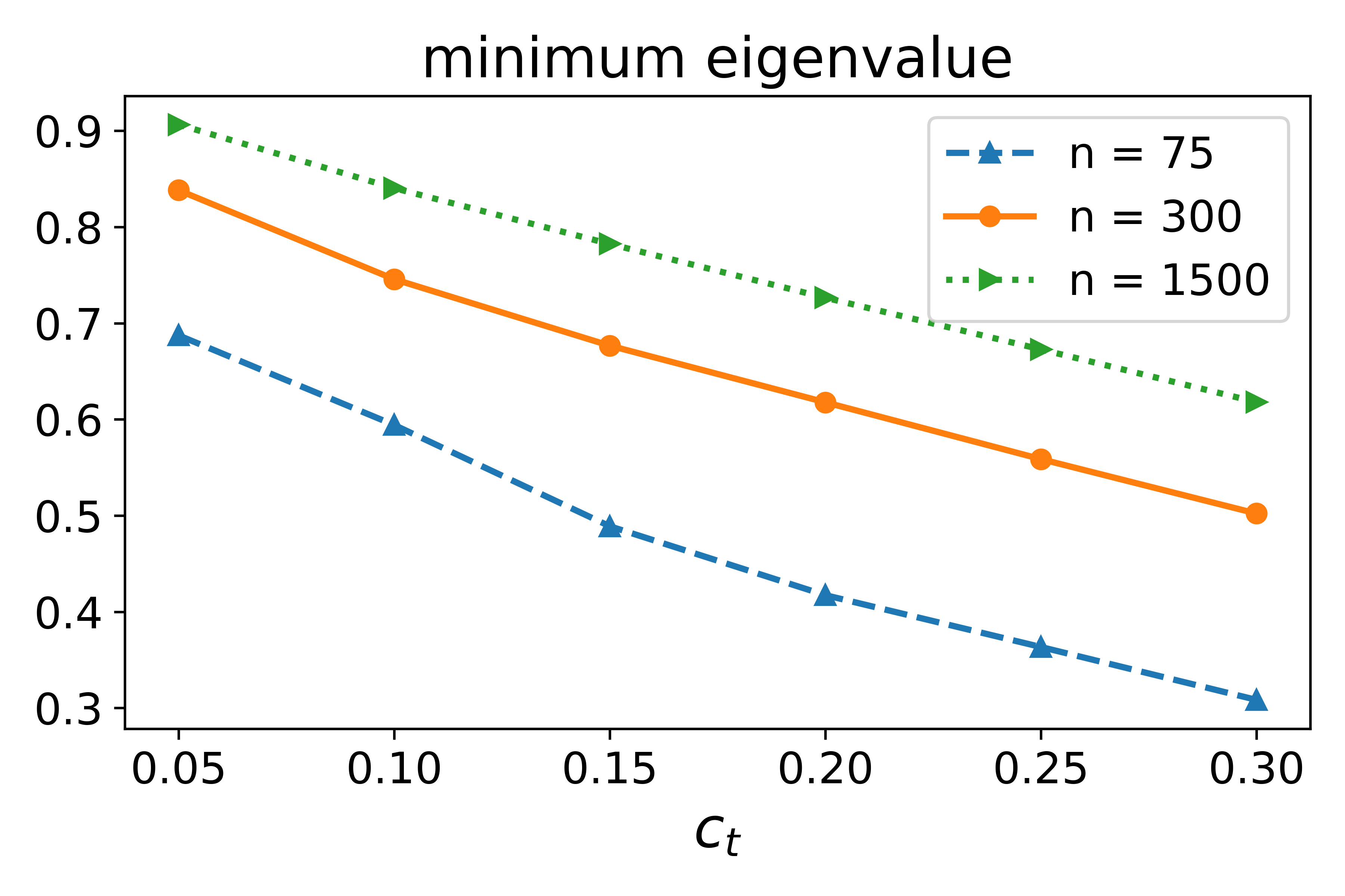
(a) Synthetic dataset

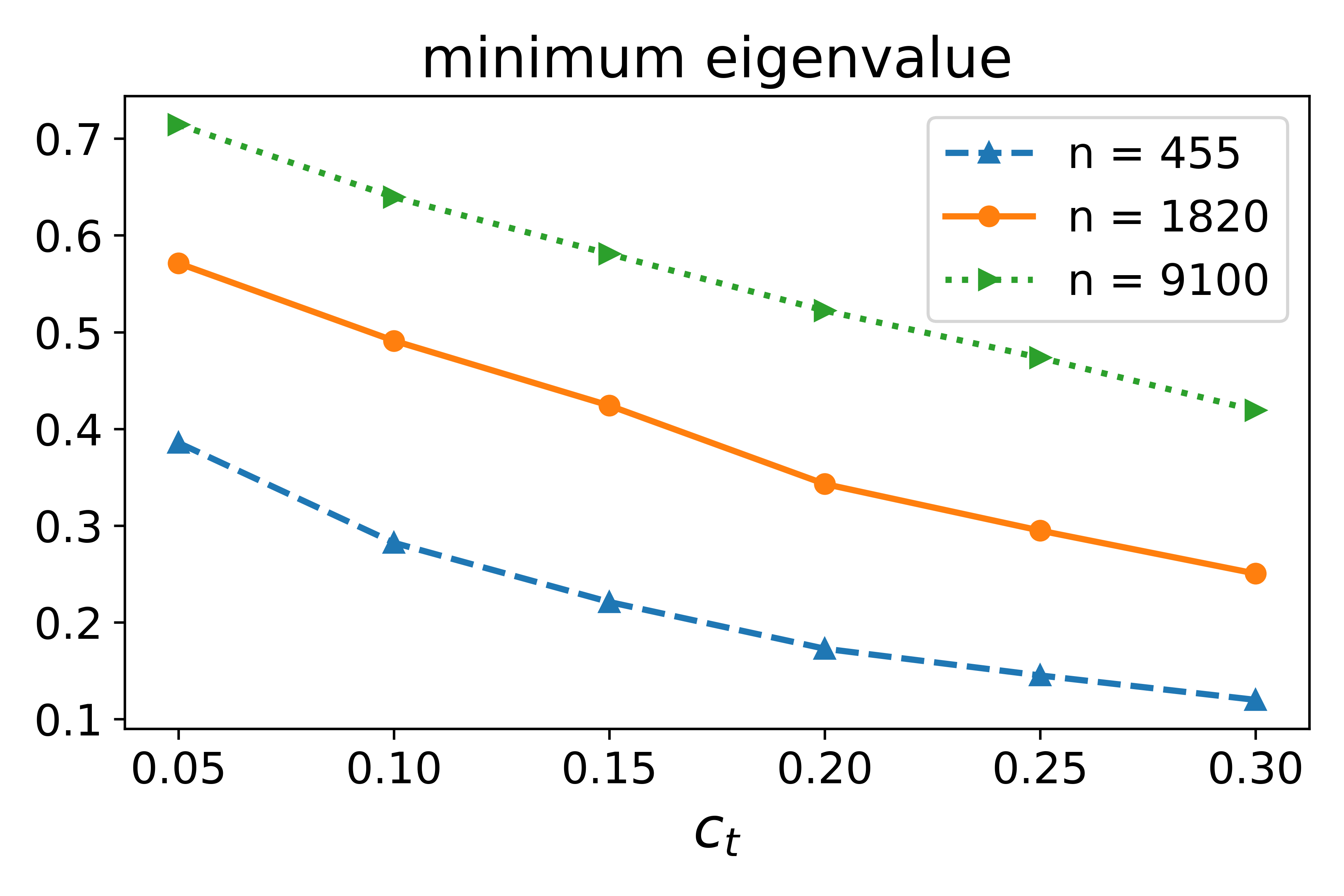
(b) YearPredictionMSD dataset

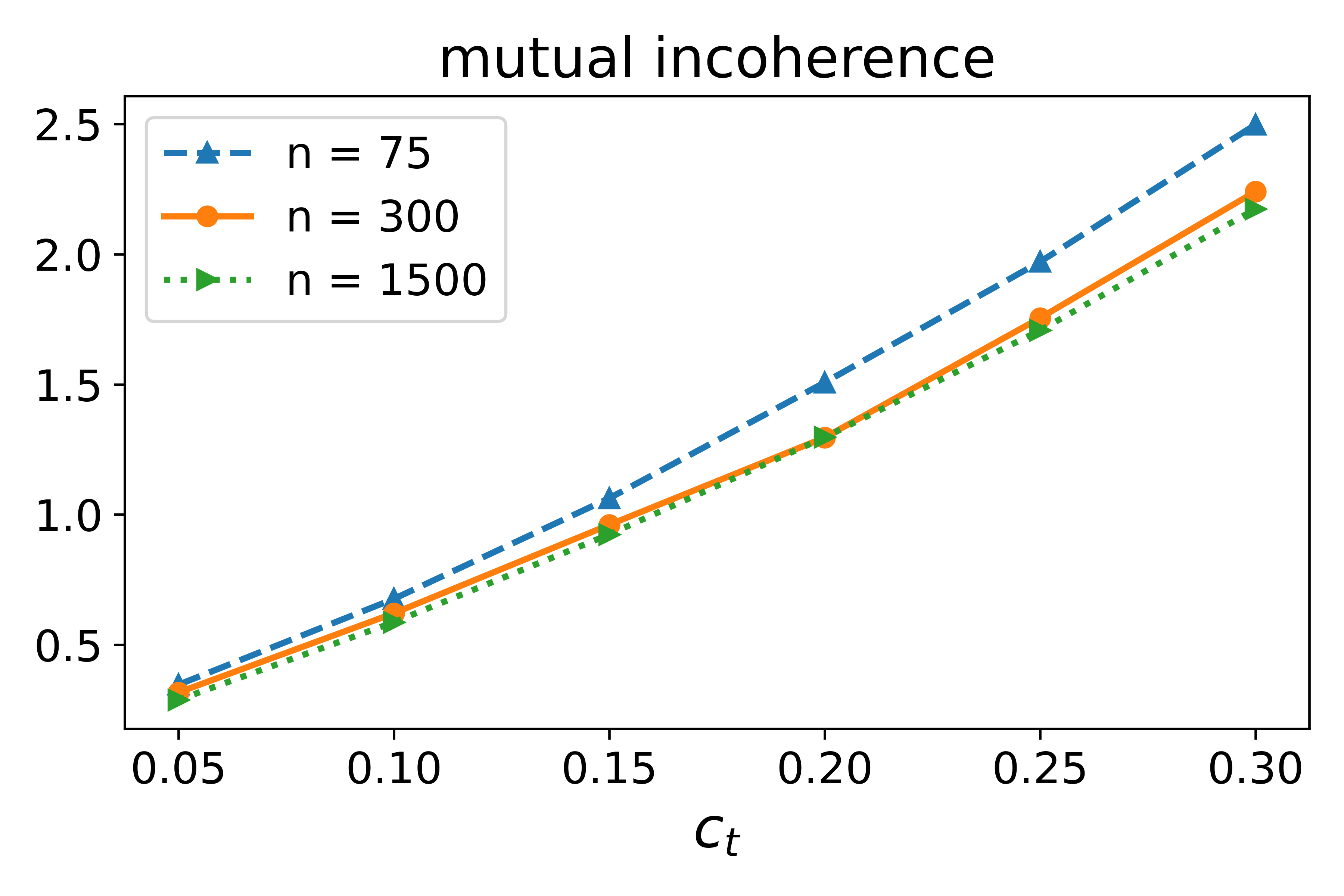
(c) Synthetic dataset

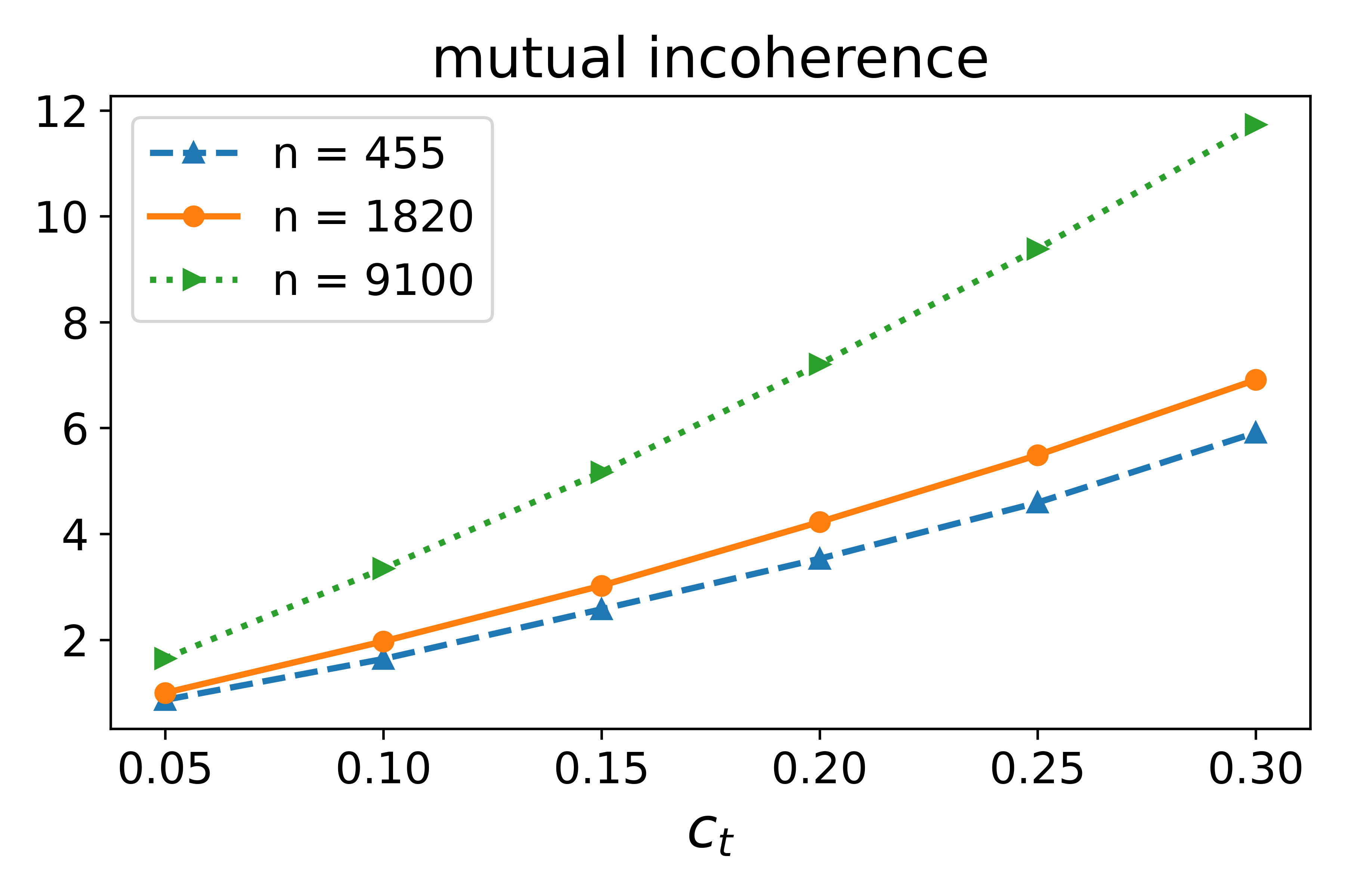
(d) YearPredictionMSD dataset

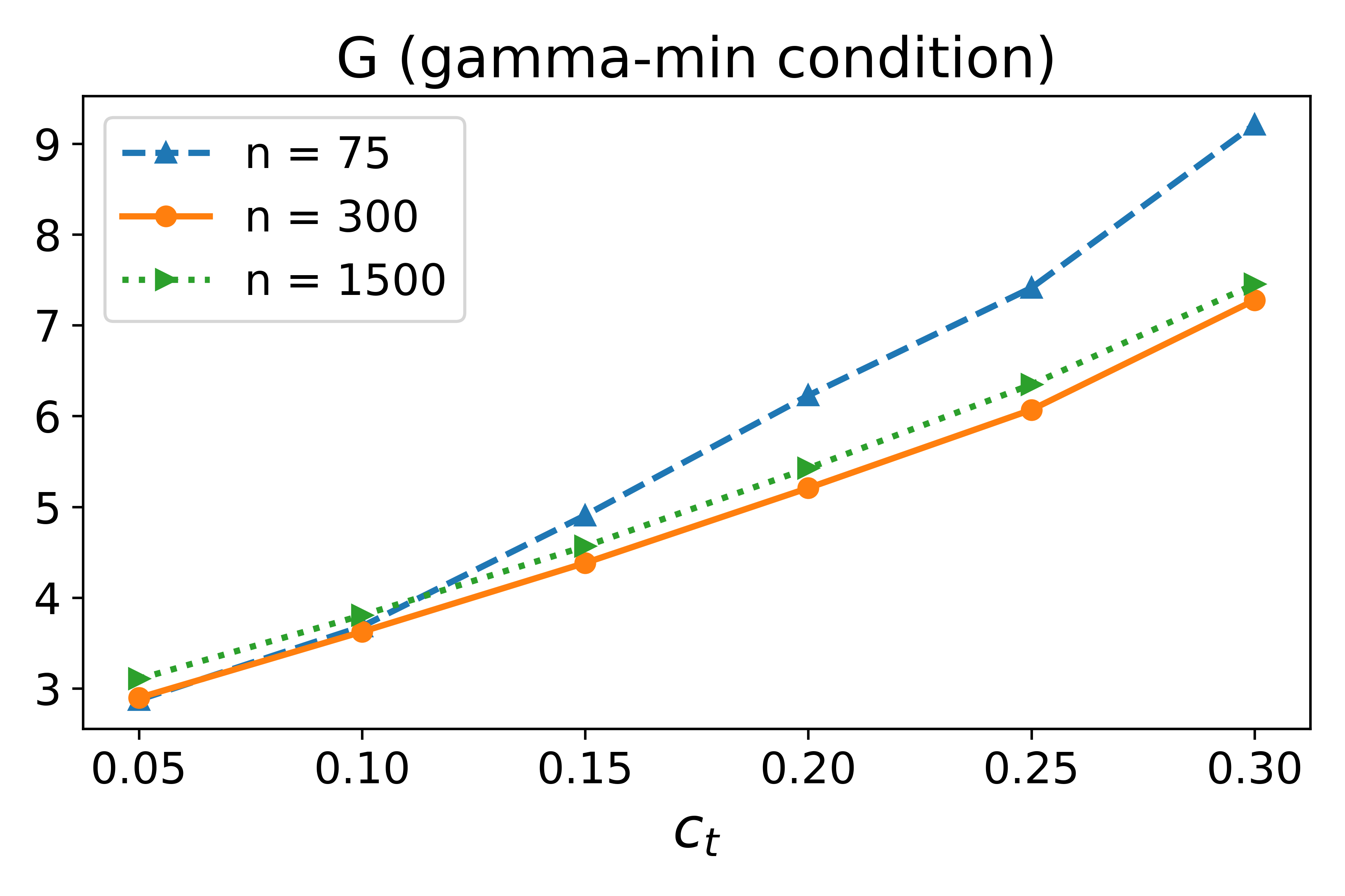
(e) Synthetic dataset

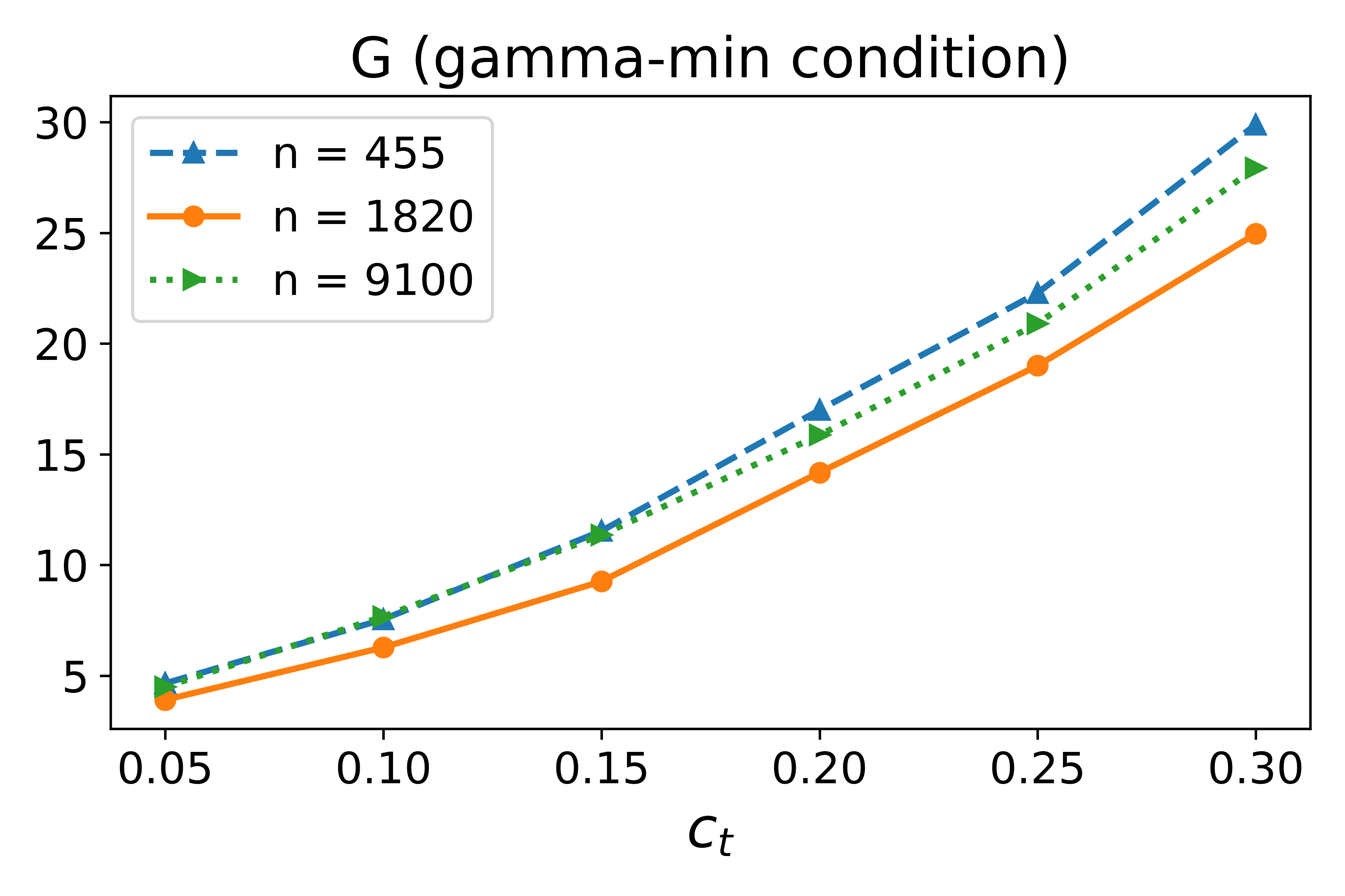
(f) YearPredictionMSD dataset

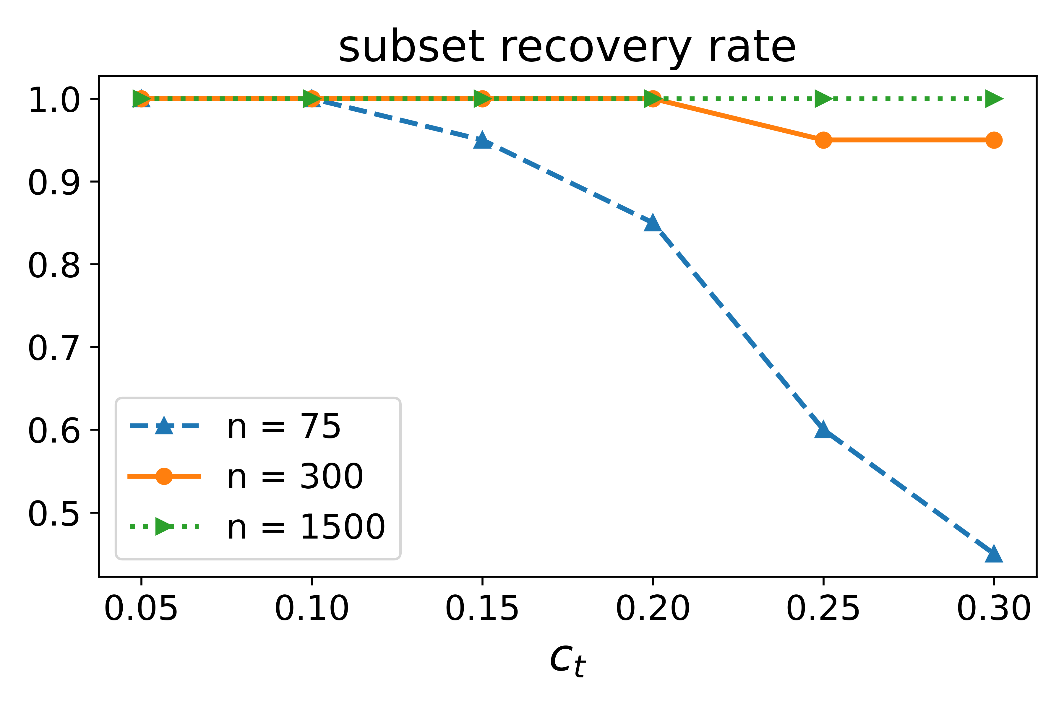
(g) Synthetic dataset

(h) YearPredictionMSD dataset

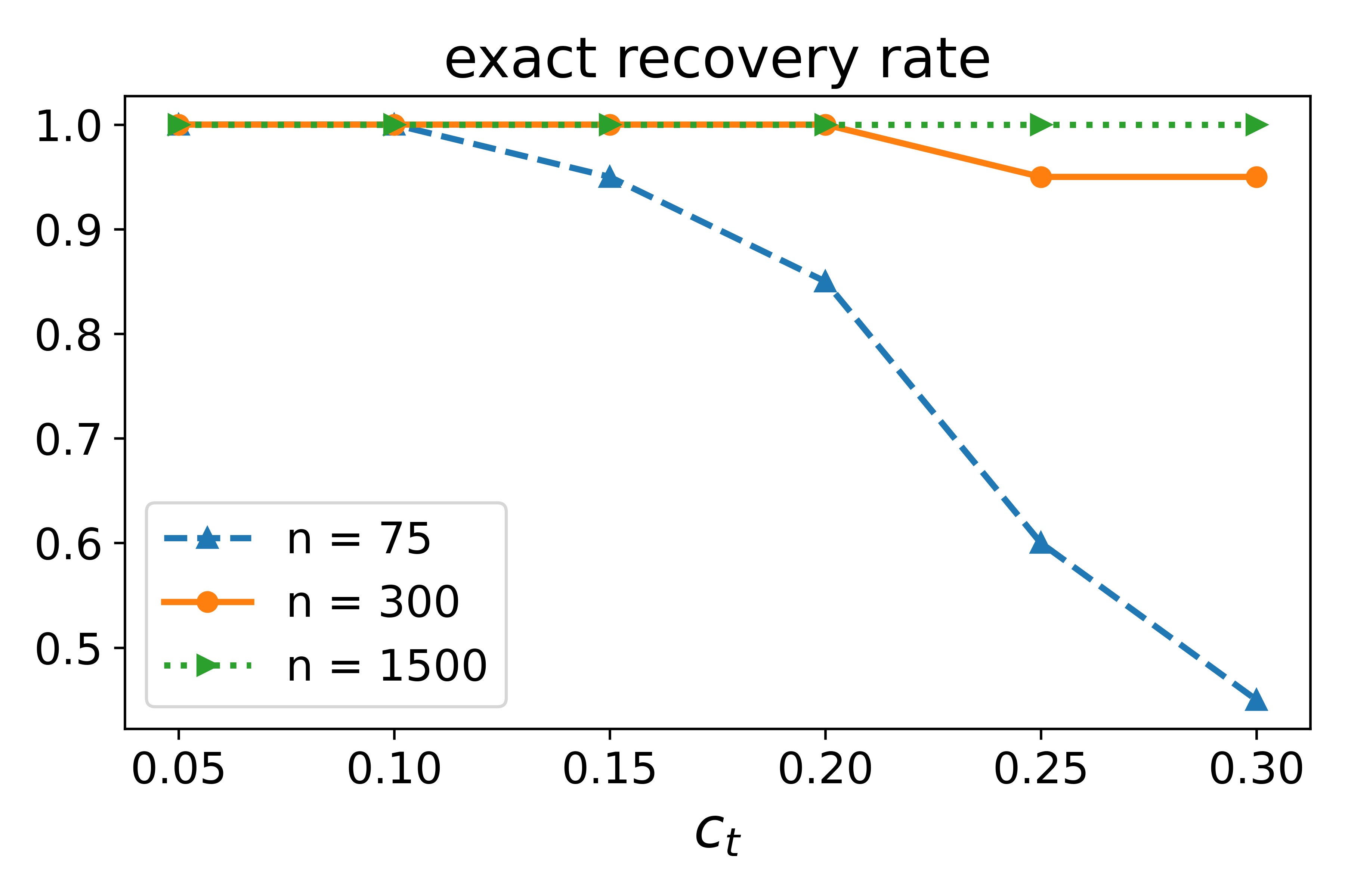
(i) Synthetic dataset

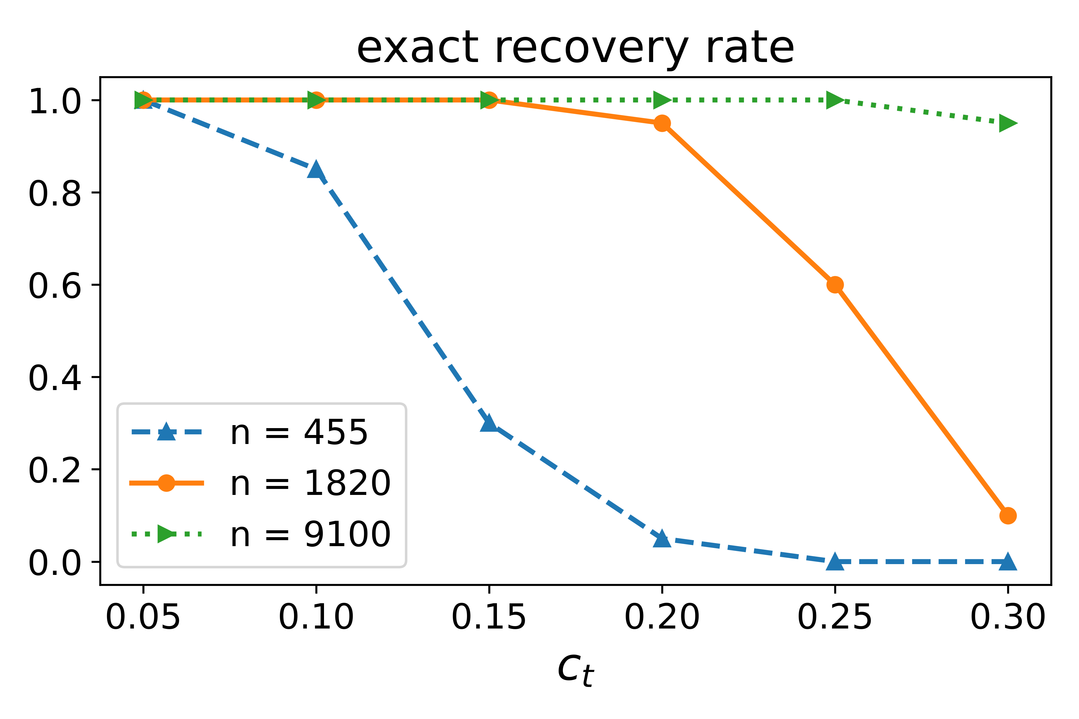
(j) YearPredictionMSD dataset

(a) Combined Cycle Power Plant dataset

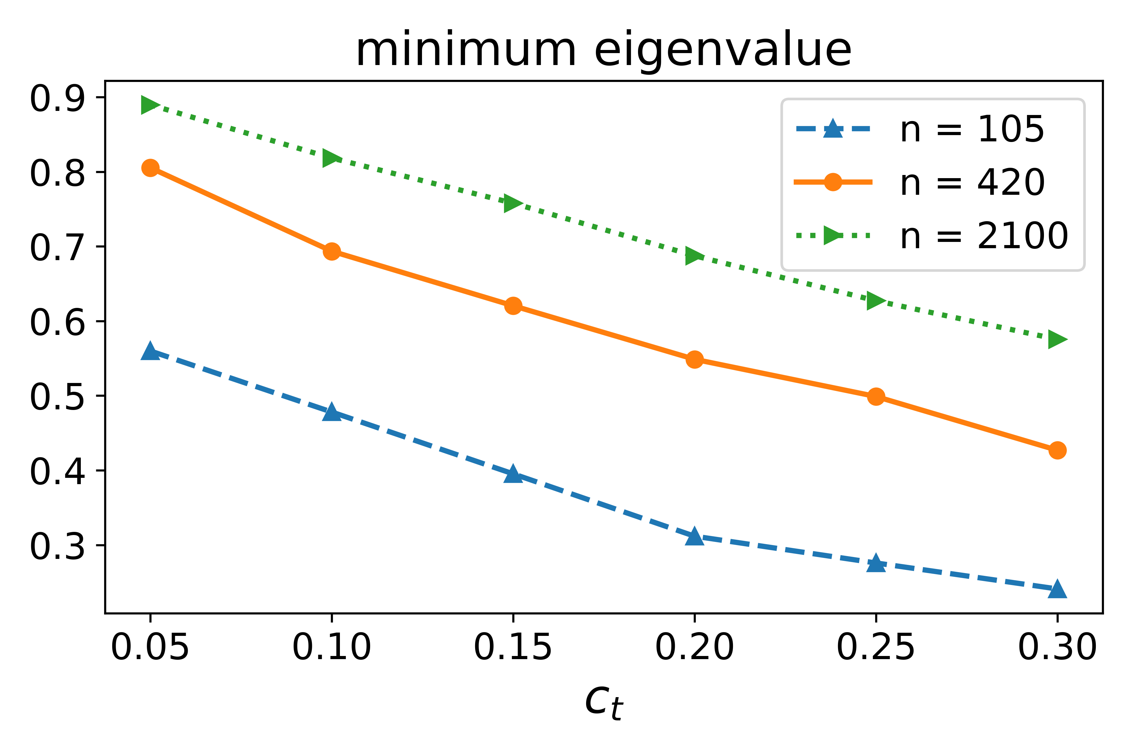
(b) Temperature forecast dataset

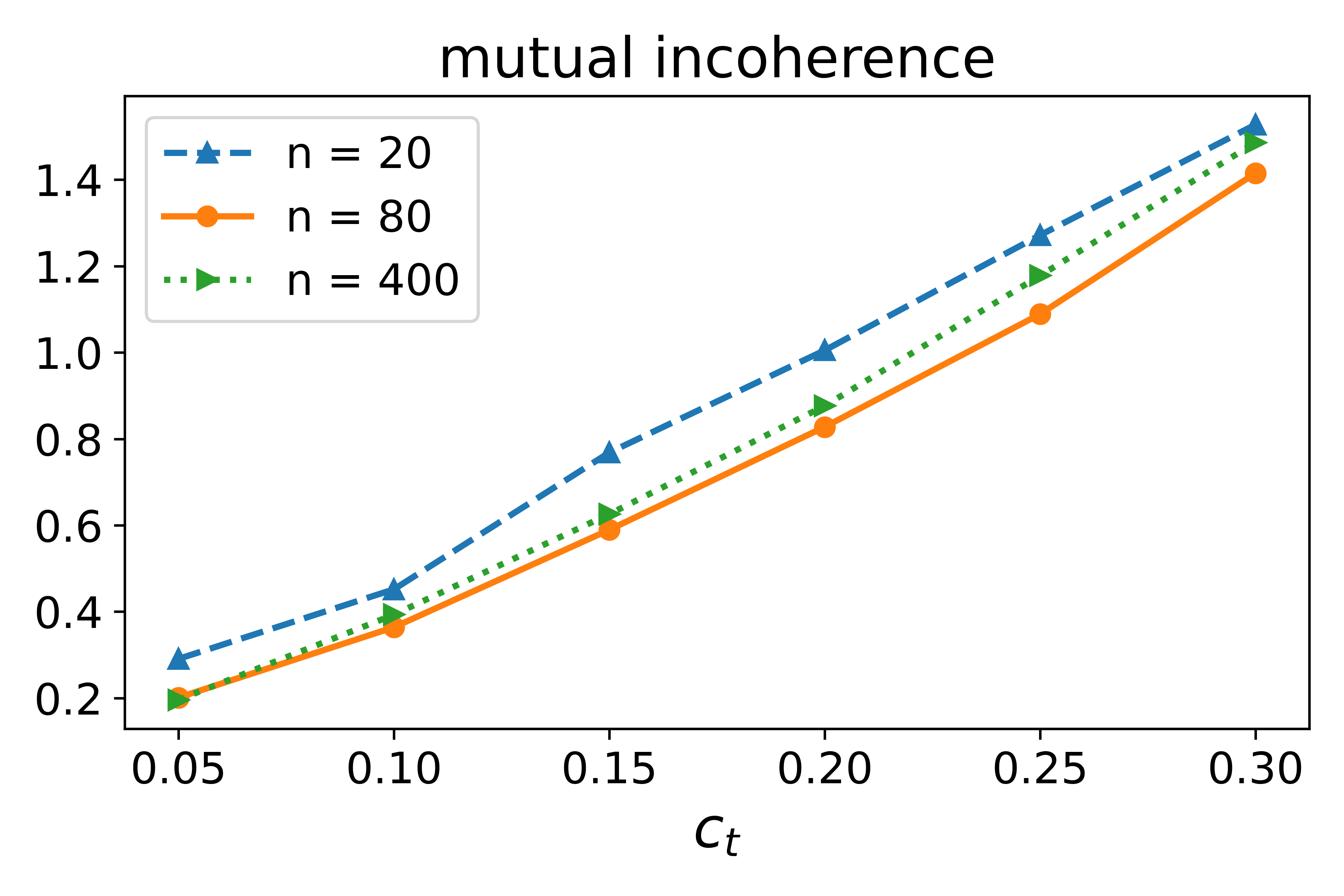
(c) Combined Cycle Power Plant dataset

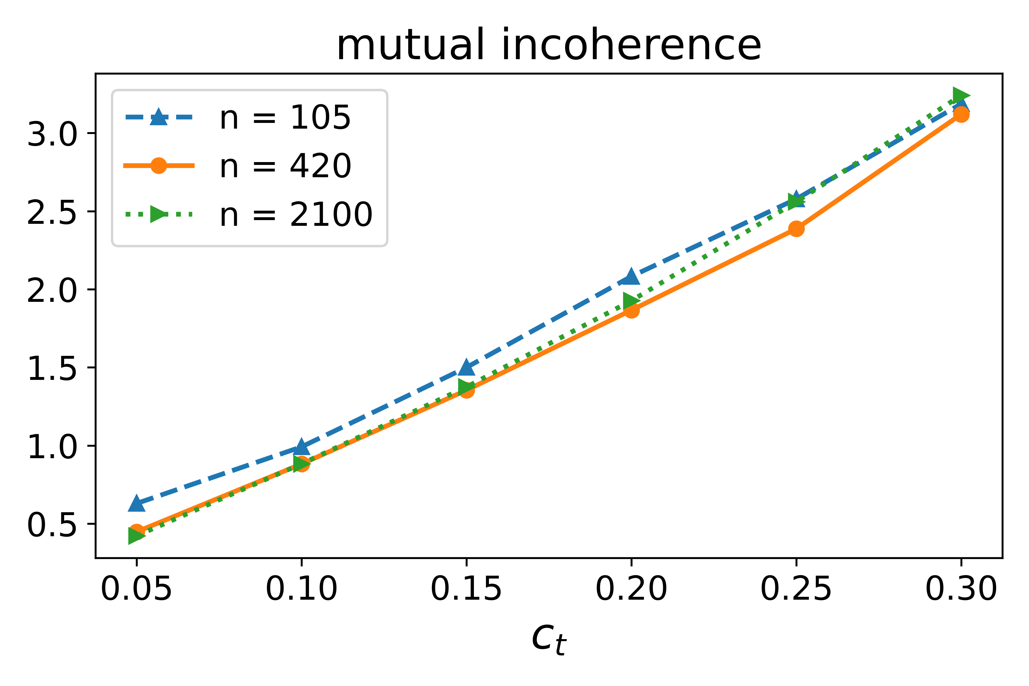
(d) Temperature forecast dataset

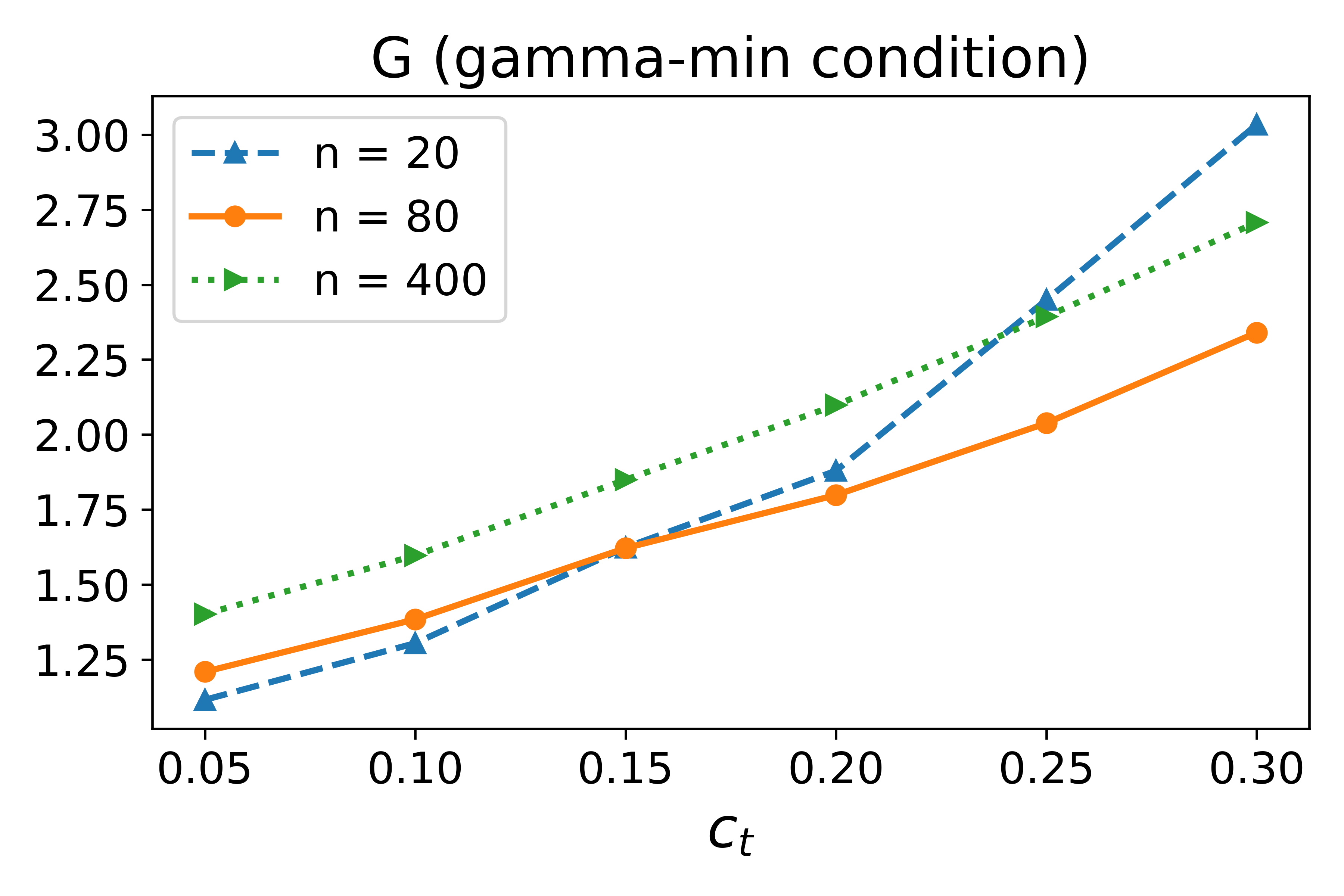
(e) Combined Cycle Power Plant dataset

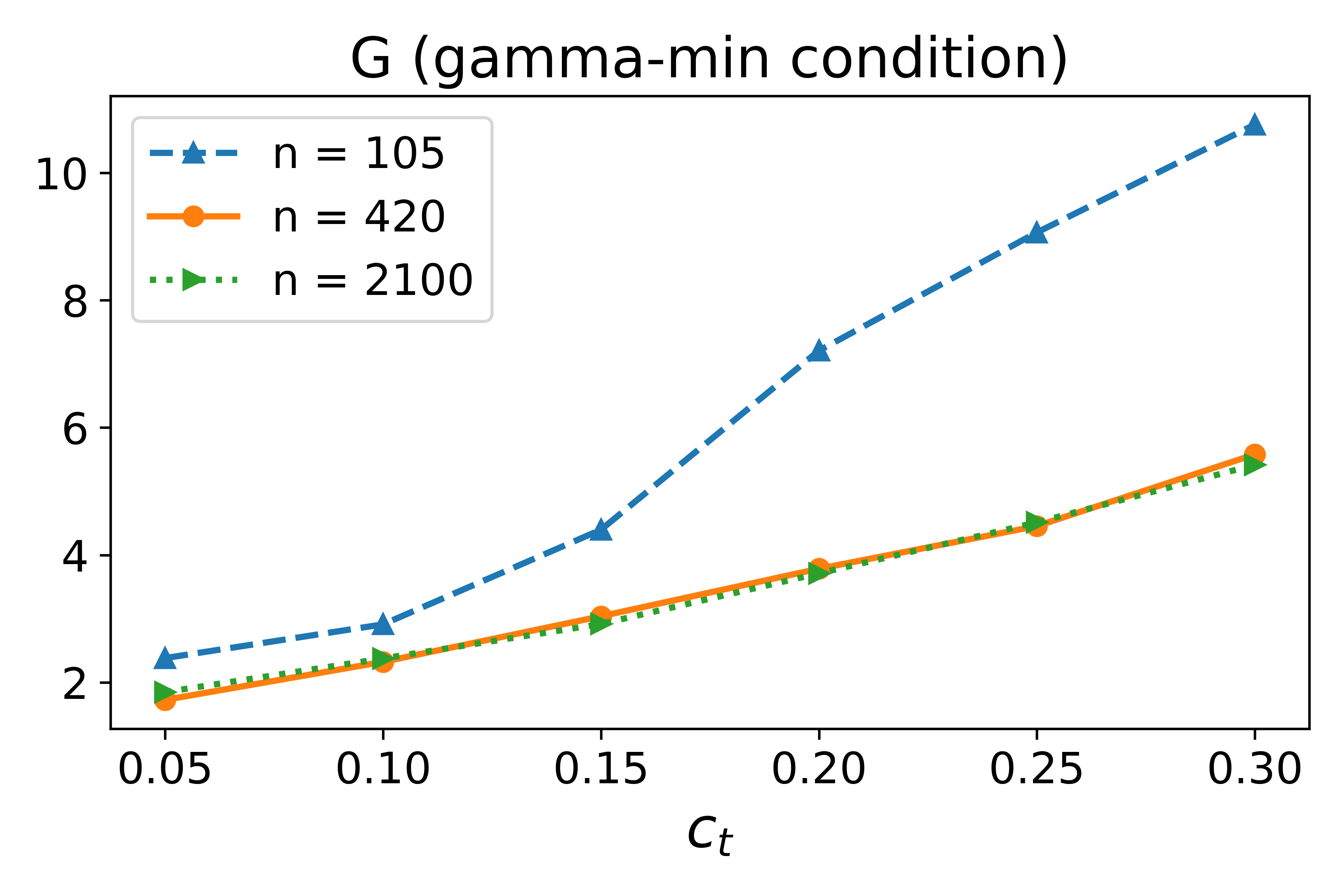
(f) Temperature forecast dataset

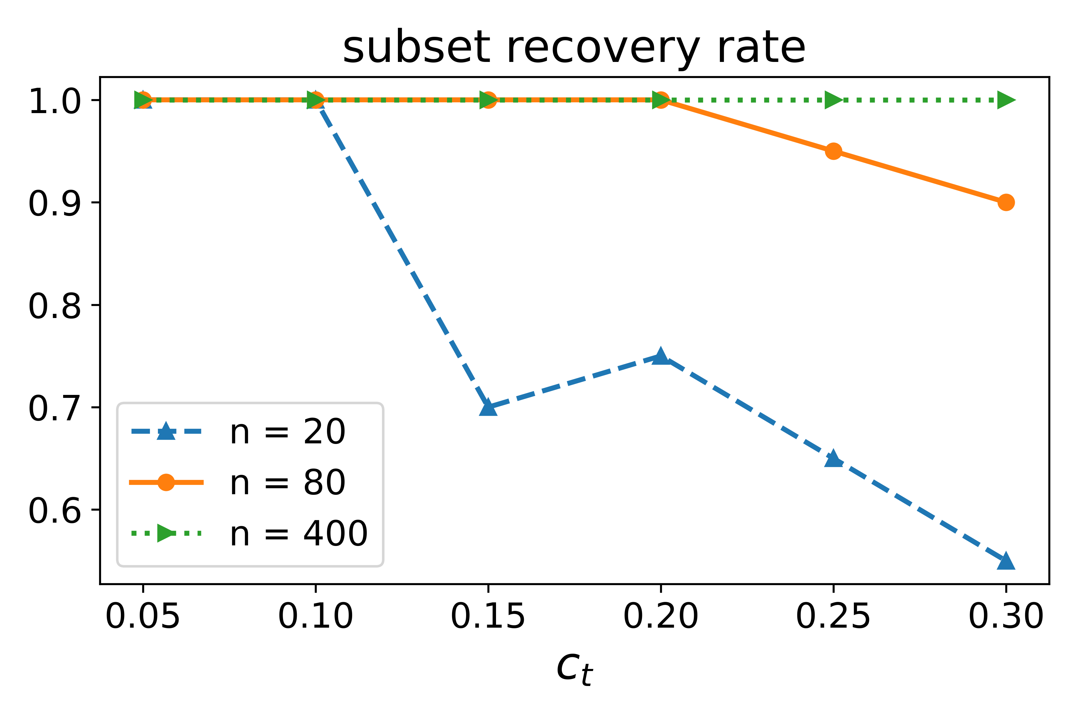
(g) Combined Cycle Power Plant dataset

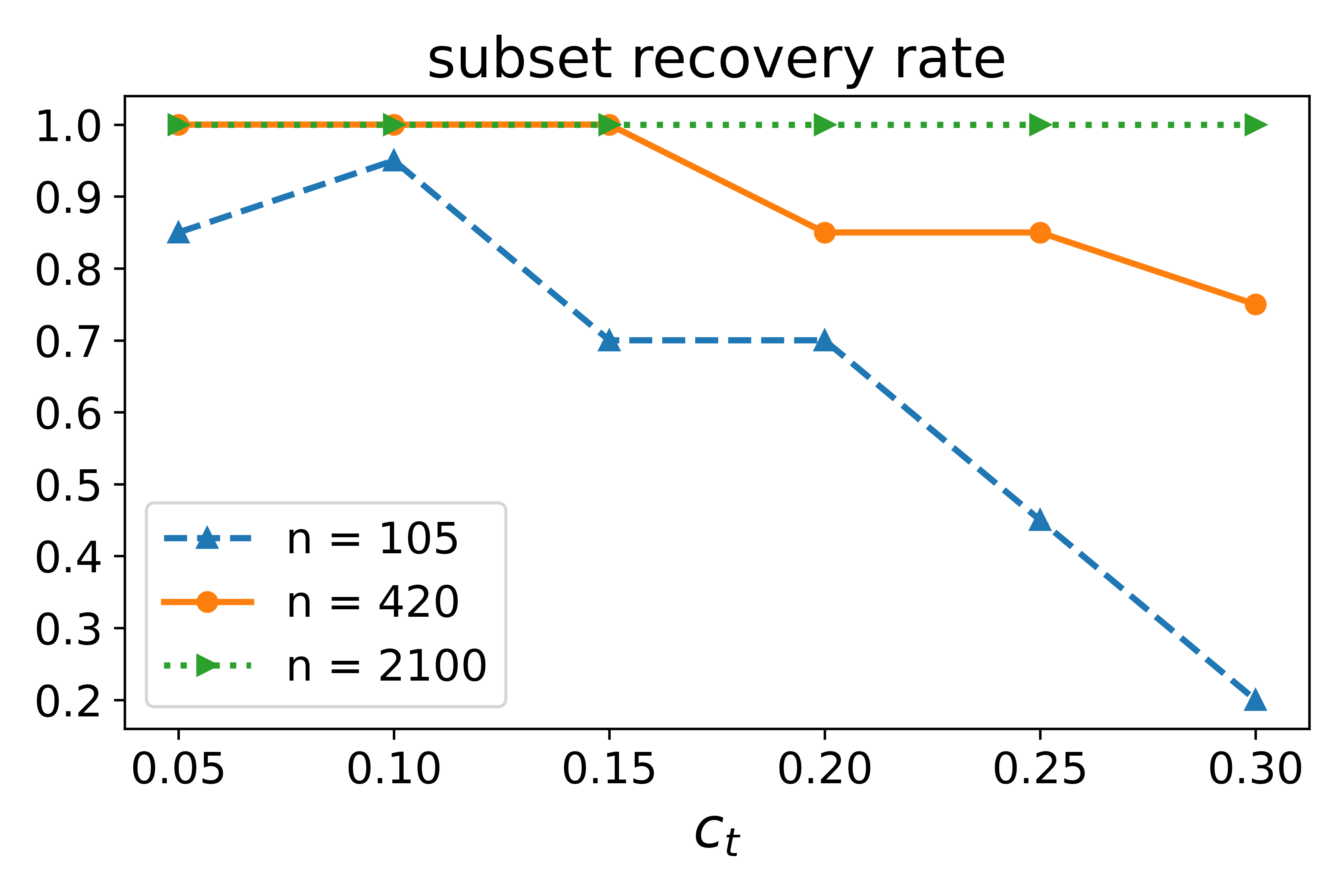
(h) Temperature forecast dataset

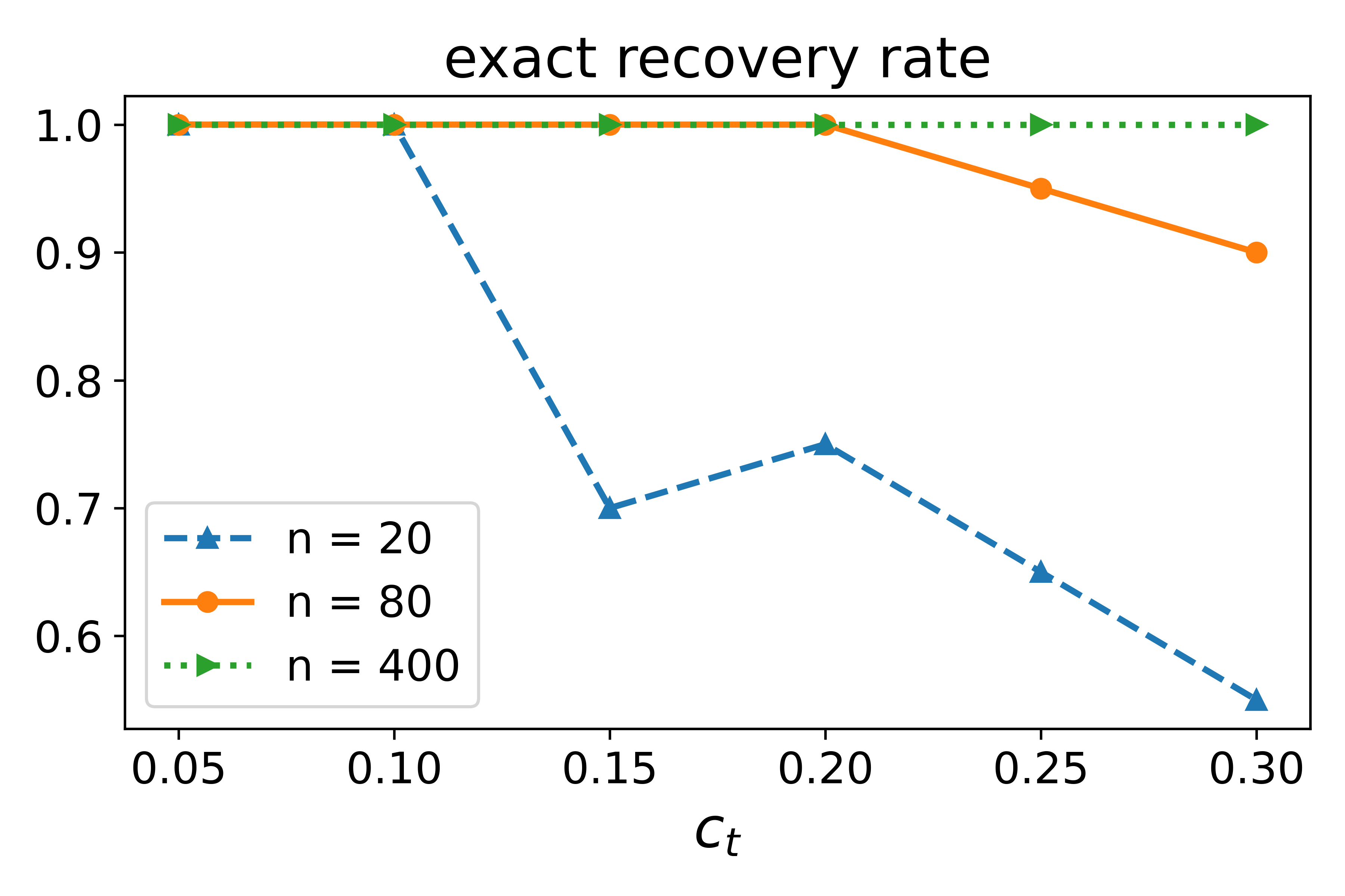
(i) Combined Cycle Power Plant dataset

(j) Temperature forecast dataset

Figure 2: Five Measurements on Four Datasets. Three different $n$’s are of values $5p,\ 20p$, and $100p$. The variance $\sigma$ is set to 0.1. The tuning parameter is set to $\lambda=2\frac{\sqrt{\log 2(n-t)}}{n}$. Each dot is an average value of 20 random trials.

The results are displayed in Figure 2. For the minimum eigenvalue assumption, a key observation from all datasets is that the minimum eigenvalue becomes larger (improves) as $n$ increases, and becomes smaller as $c_{t}$ increases. For the mutual incoherence assumption, the synthetic dataset satisfies the condition with less than 15% outliers. The Combined Cycle Power Plant dataset has mutual incoherence close to 1 when $c_{t}$ is approximately 20%-25%, and the mutual incoherence condition of the YearPredictionMSD dataset approaches 1 when $c_{t}$ is approximately 5%. Therefore, we see that the validity of the assumption highly depends on the design of $X$. For the gamma-min condition, as $c_{t}$ increases, we need more obvious (larger $\min_{i}|\gamma^{*}_{i}|$) outliers. Finally, with larger $n$ and smaller $c_{t}$, the subset/exact recovery rate improves.

6.1.2 Effectiveness for Recovery

The second experiment compares our debugging method to other proposed methods in the robust statistics literature. We compare our method with the Fast LTS [rousseeuw2006computing], E-lasso [nguyen2013robust], Simplified $\Theta$-IPOD [she2011outlier], and Least Squares methods. E-lasso is similar to our formulation, except it includes an additional penalty with $\beta$. The Simplified $\Theta$-IPOD method iteratively uses hard thresholding to eliminate the influence of outliers. For the experimental setup, we generate synthetic data with $n=2000,t=200,p=15$, and $\sigma=0.1$, but replace step [S4] by one of the following mechanisms for generating $\gamma^{*}$:

1. We generate $\gamma^{*}_{i},i\in T$ by $Bernoulli(\pm 1,0.5)\cdot(10\sqrt{\log(2n)\sigma}+Unif(0,10))$.

2. We generate $\beta^{\prime}$ elementwise from $Unif(-10,10)$ and take $\gamma^{*}_{i}=x_{i}^{\top}(\beta^{\prime}-\beta^{*}),i\in T$.

The first adversary is random, whereas the second adversary aims to attack the data by inducing the learner to fit another hyperplane. The precision/recall for Fast LTS and Least Squares are calculated by running the method once and applying various thresholds to clip $\widehat{\gamma}$. For the other three methods, we apply different tuning parameters, compute precision/recall for each result, and finally combine them to plot a macro precision-recall curve.

In the left panel of Figure 3, Least Squares and Fast LTS reach perfect AUC, while the other three methods have slightly lower scores. In the right panel of Figure 3, we see that debugging, E-lasso, and Fast LTS perform comparably well, and slightly better than Simplified $\Theta$-IPOD. Not surprisingly, Least Squares performs somewhat worse, since it is not a robust procedure.

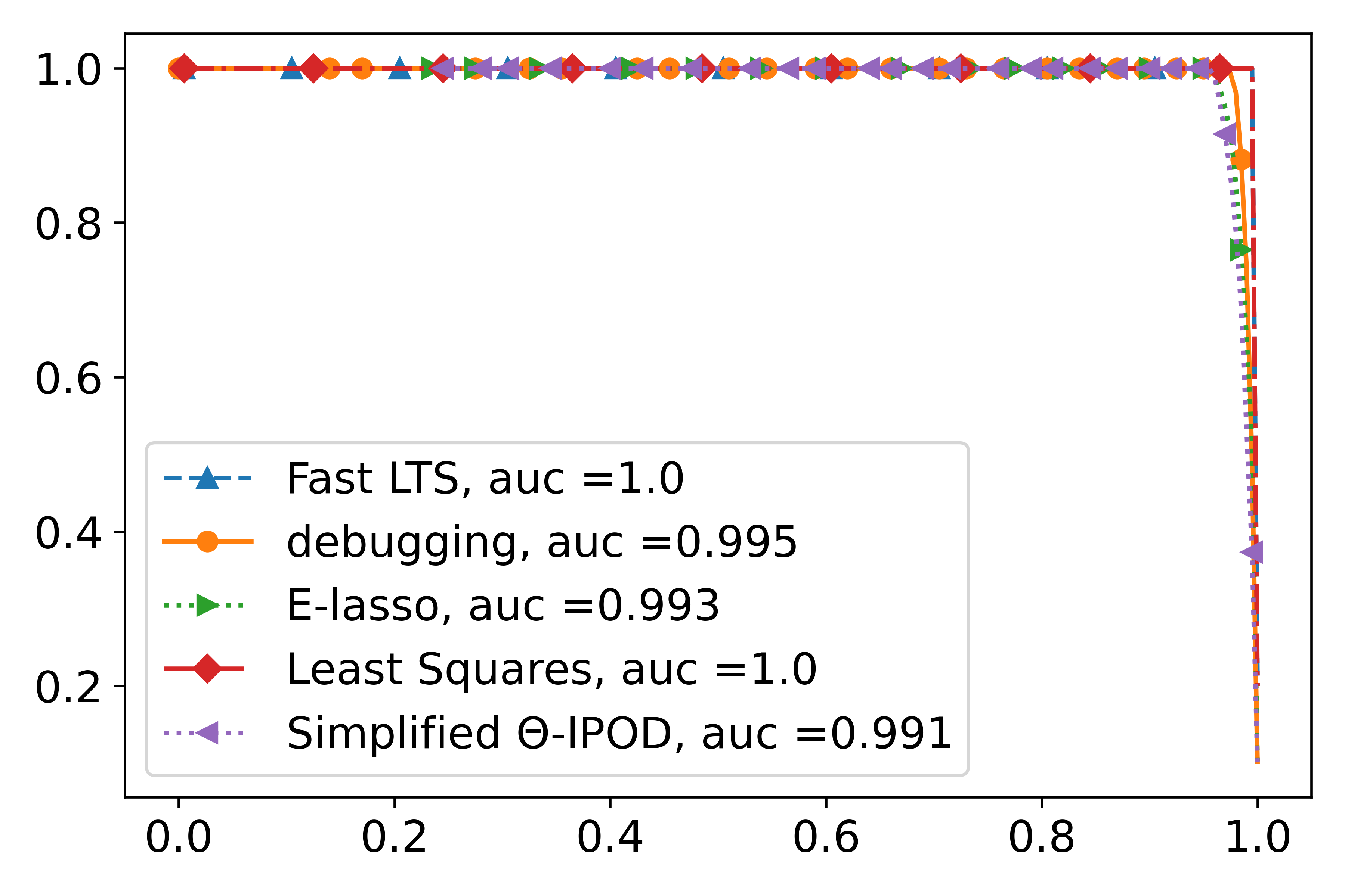
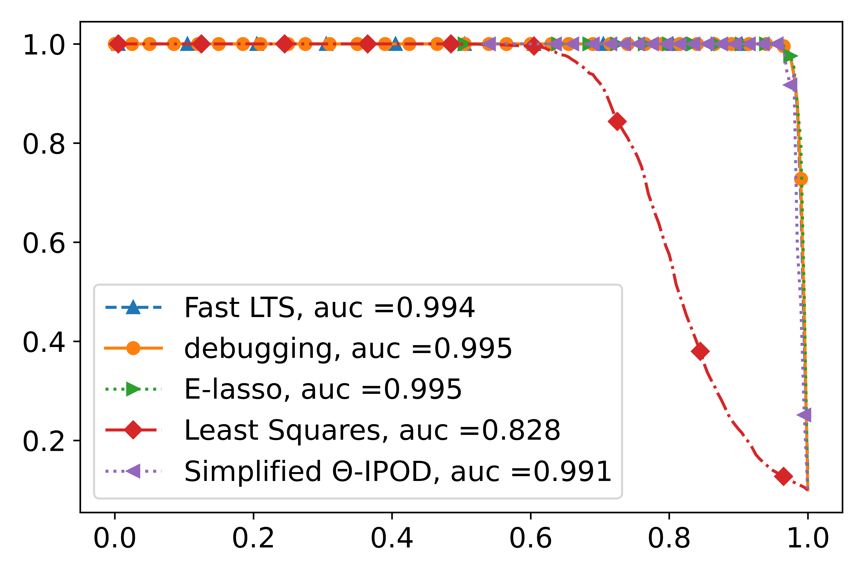
Figure 3: Precision Recall Curves over Different Regression Methods. The two plots correspond to the two settings described in the text for generating $\gamma^{*}$. To better view the curves, we only show the dots for every $c$ positions, where $c$ is an interger and different for different methods.

6.2 Tuning Parameter Selection

We now present two experimental designs for tuning parameter selection. The first experiment runs Algorithm 1 for both one- and two-pool cases. We will present the recovery rates for a range of $n$’s and $c_{t}$’s, showing the effectiveness of our algorithm in a variety of situations. The second experiment compares Algorithm 1 in one- and two-pool cases to cross-validation, which is a popular alternative for parameter tuning. Our results indicate that Algorithm 1 outperforms cross-validation in terms of support recovery performance.

We begin by describing the method used to generate the second data pool. Given the first data pool $(X,y)$ and the ground-truth parameters $(\beta^{*},\sigma)$, we describe two pipelines to generate the second pool. The first pipeline checks $m$ random points of the first pool, with steps [T1-T3]:

1. Select $m$ points uniformly at random from the first pool to construct $\widetilde{X}$ for the second pool.

2. Generate $\widetilde{\epsilon}\in{}^{m}$, where each entry $\widetilde{\epsilon}_{i}$ is drawn i.i.d. from $\mathcal{N}(0,\sigma^{2}/L)$.

3. Generate the labels by $\widetilde{y}=\widetilde{X}\beta^{*}+\widetilde{\epsilon}$.

When the debugger is able to query features of clean points from a distribution $\mathcal{P}_{X}$, we can use a second pipeline, where [T1] is replaced by [T1’]:

1. Independently draw $m$ points from $\mathcal{P}_{X}$ to construct $\widetilde{X}$.

6.2.1 Verification of Algorithm 1

We use the default procedure for generating the synthetic dataset, with parameters $p=15$, $\sigma=0.1$, and $t=c_{t}n$, where $c_{t}$ ranges from 0.05 to 0.4 in increments of 0.05. In all cases, we input $\bar{c}=0.2$ and $\lambda_{u}=\frac{2\|P_{X}^{\perp}y\|_{\infty}}{n}$ in Algorithm 1.

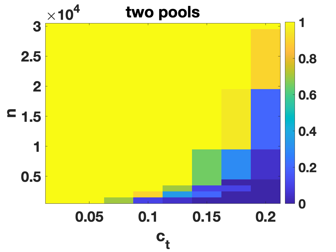
Figure 4: Exact Recovery Rate over 20 Trials. The recovery rate is shown in different cases varying by fraction of outliers $c_{t}$ and $n$. The left subfigure is for one-pool case and the right subfigure is for two-pool case. We set $m=100,L=5$ for the second pool.

Figure 4 displays the results for $n\in\{1,2,3,4,5,10,20,30\}\cdot 10^{3}$. First, we see that Algorithm 1 achieves exact support recovery in all 20 trials in the yellow area. Second, the exact recovery rate increases with increasing $n$ and decreasing $c_{t}$, showing that the algorithm is particularly useful for large-scale data sets. This trend can also be seen from the requirement on $n$ imposed in Theorem 7. In particular, we see that the contour curve for the exact recovery rate matches the curve of $\left(1-c_{t}\right)^{-\frac{1}{1-2c_{n}}}$ for some constant $c_{n}\in(0,\frac{1}{2})$. However, a downside of Algorithm 1 is that it does not fully take advantage of the second pool in the two-pool case, as the left panel and the right panel display similar results.

6.2.2 Effectiveness of Tuning Parameter Selection

We now compare our method for tuning parameter selection to cross-validation. We also use the postprocessing step described at the beginning of the section. Four measurements are presented, including two recovery rates, the $\ell_{2}$-error of $\widehat{\beta}$, and the runtime. In both the one- and two-pool cases, we use our default methods for generating synthetic data, and we set $\bar{c}=0.2$ for all the experiments.

The cross-validation method for the one-pool case splits the dataset into training and testing datasets with the ratio of $8:2$, then selects $\lambda$ with the smallest test error, $\|X_{test}\widehat{\beta}-y_{test}\|_{2}$. The procedure for the two-pool case is to run the Lasso-based debugging method with a list of candidate $\lambda$’s and test it on the second pool. Finally, we select the $\lambda$ value with the smallest test error, $\|\widetilde{X}\widehat{\beta}-\widetilde{y}\|_{2}$. We use 15 candidate values for $\lambda$, spaced evenly on a log scale between $10^{-6}$ and $\lambda_{u}=\frac{2\|P_{X}^{\perp}y\|_{\infty}}{n}$.

Figure 5 compares the results in the one-pool case. We note that cross-validation does not perform very well for all the measurements except $\|\widehat{\beta}-\beta^{*}\|_{2}$. Specifically, it does not work at all for subset support recovery, since cross-validation tends to choose very small $\lambda$ values. For the $\ell_{2}$-error, we see that for small values of $c_{t}$, our algorithm can select a suitable choice of $\lambda$, so that after removing outliers, we can fit the remaining points very well. This is why the debugging + postprecessing methods gives the lowest error. As $c_{t}$ increases, our debugging method shows poorer performance in terms of support recovery, resulting in larger $\ell_{2}$-error for $\widehat{\beta}$. Although cross-validation seems to perform well, carefully designed adversaries may still destroy the good performance of cross-validation, since its test dataset could be made to contain numerous buggy points.

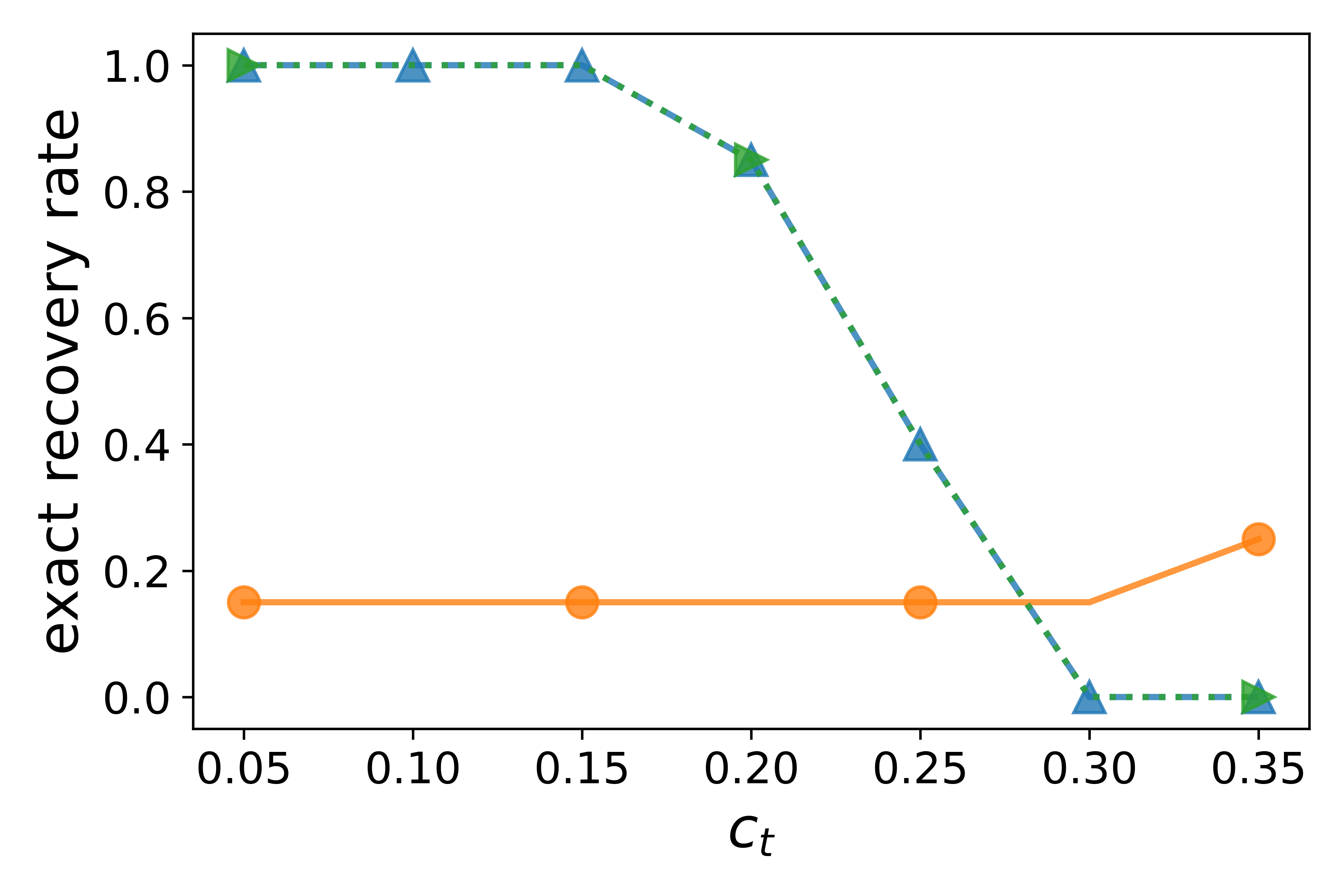
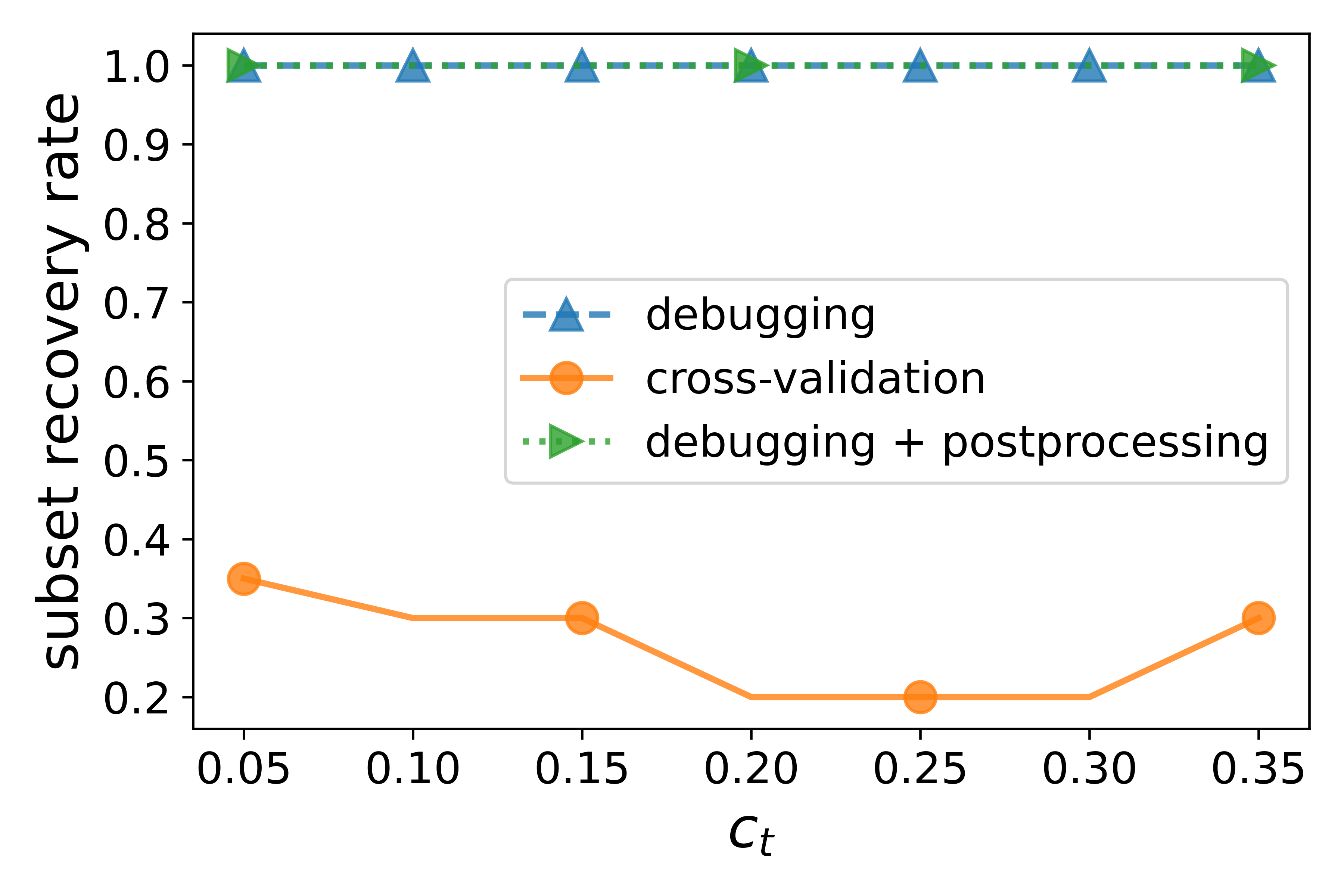
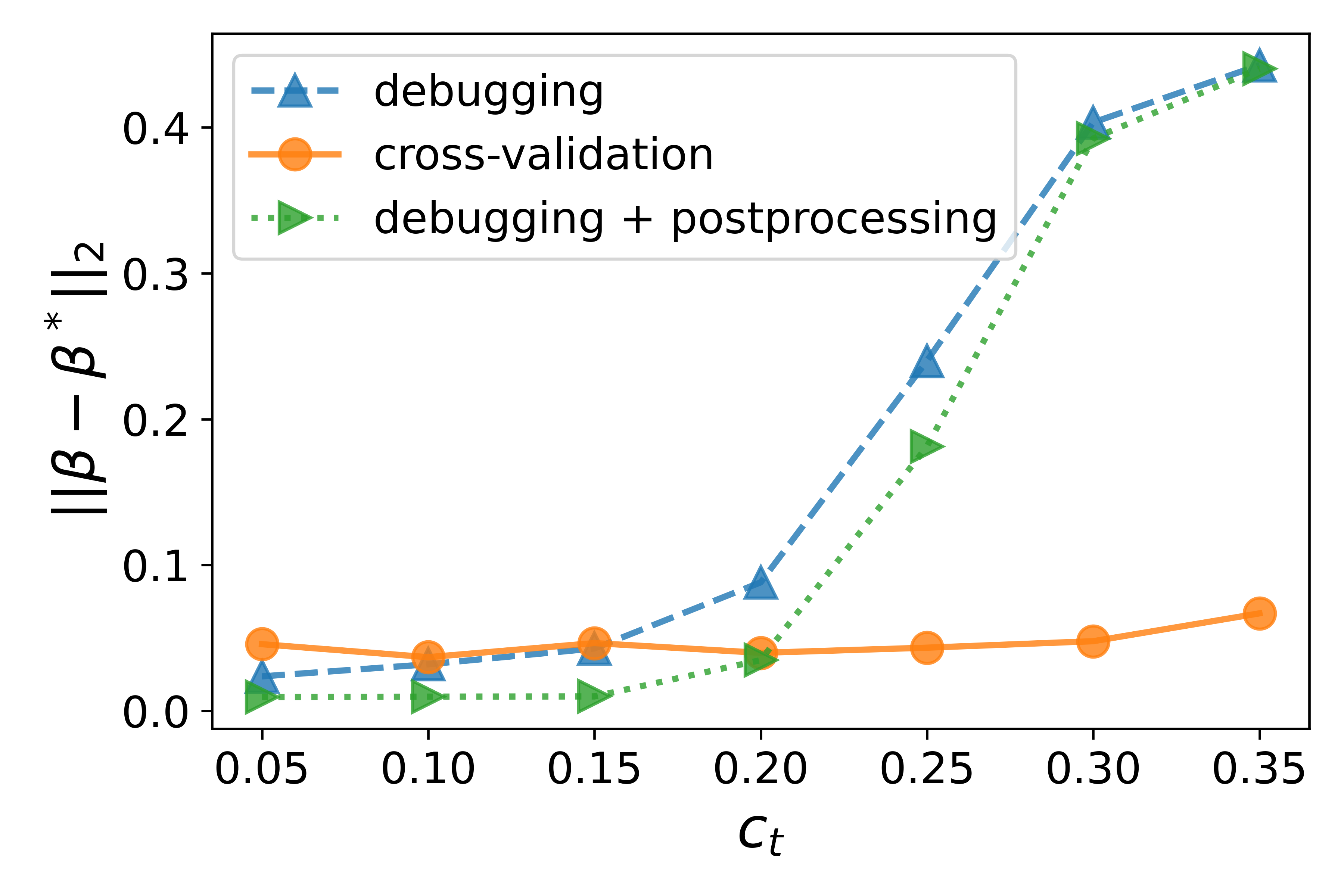
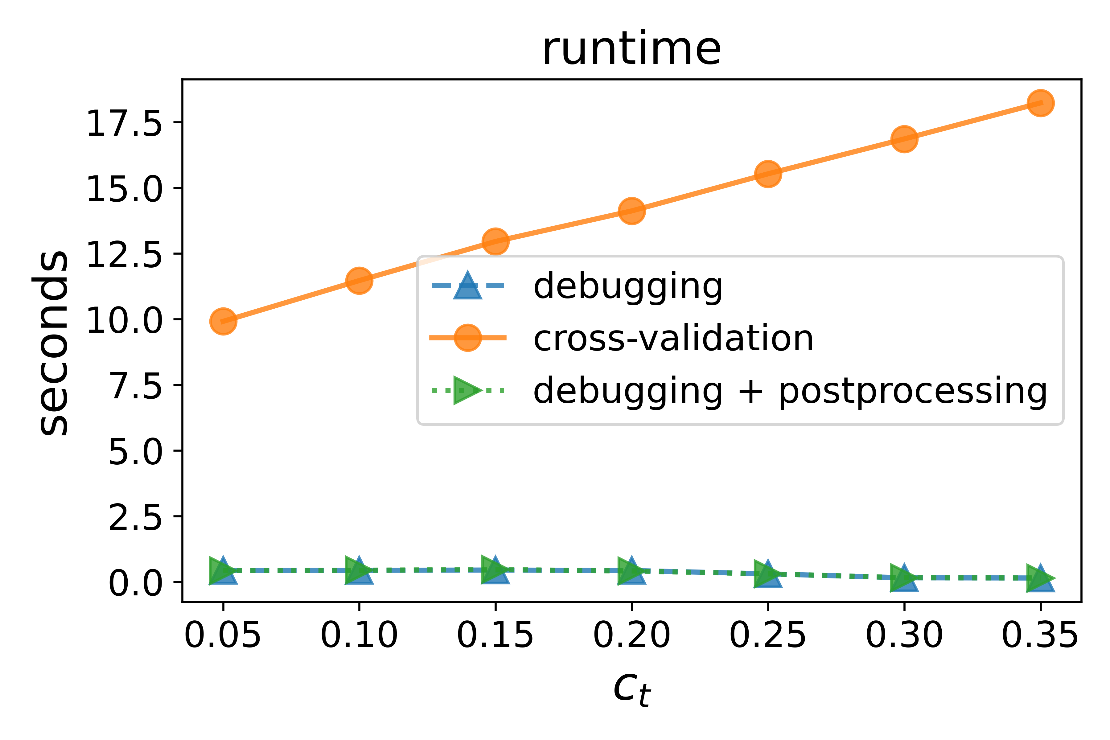
Figure 5: Effectiveness of Tuning Parameter Selection (One Pool). Each dot is the average result of 20 random trials. We set $n=2000,p=15$, and $\sigma=0.1$.

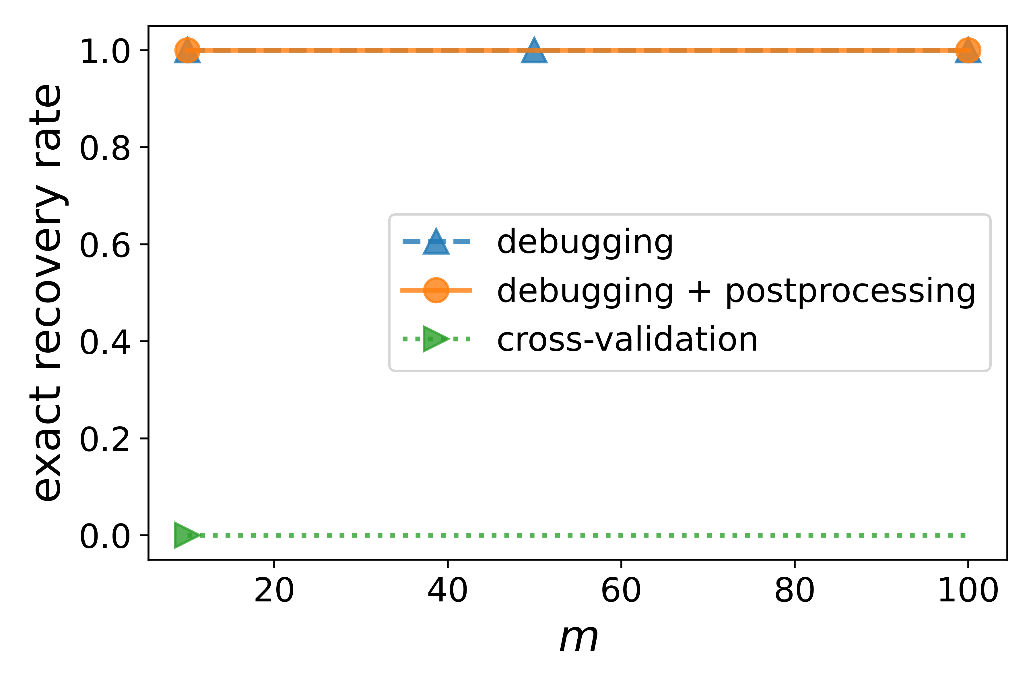
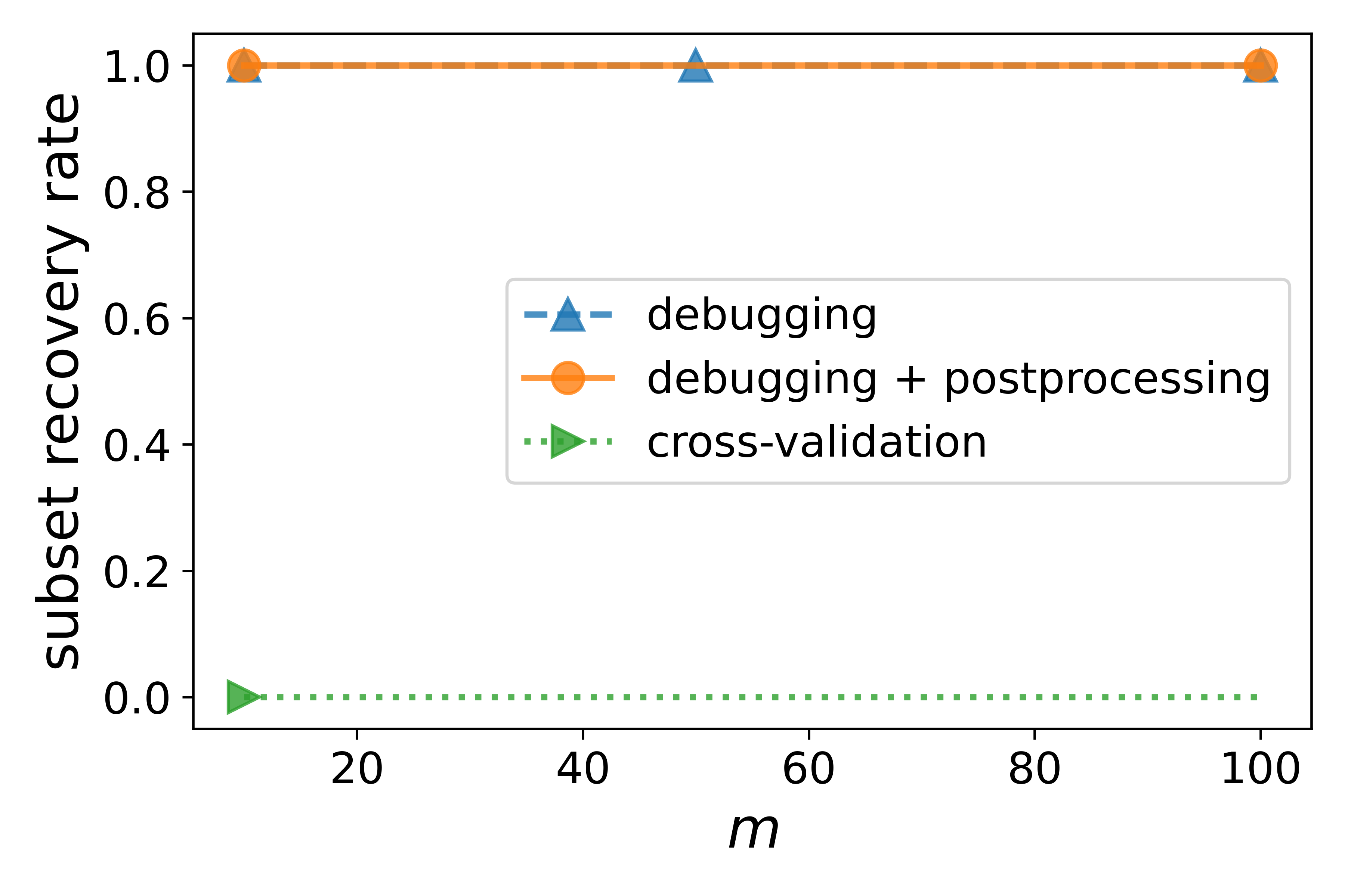
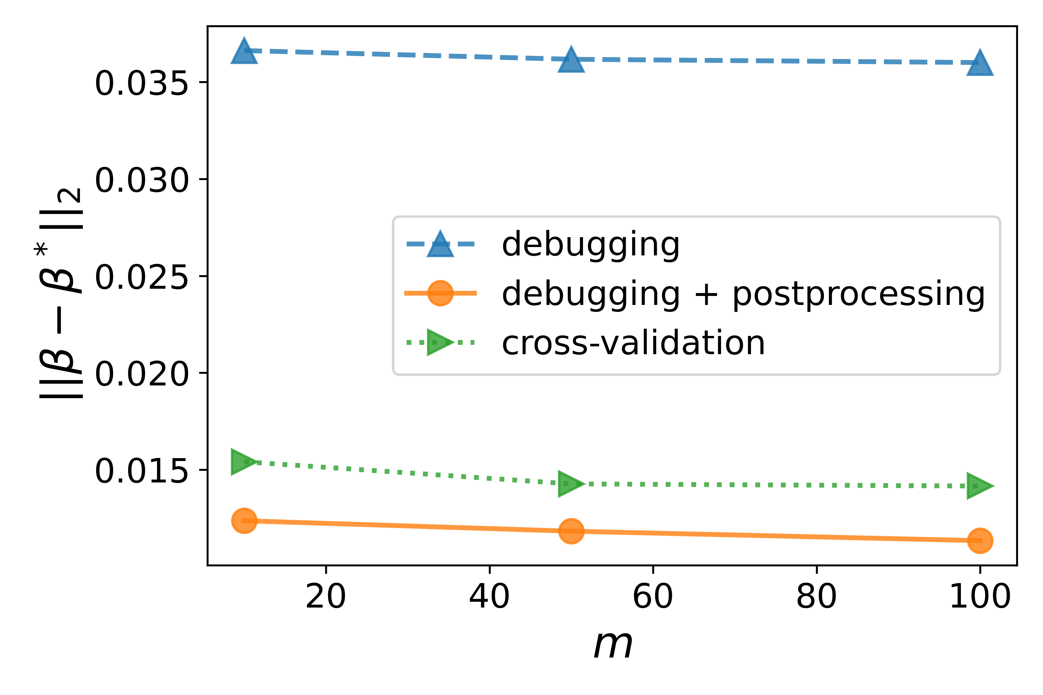
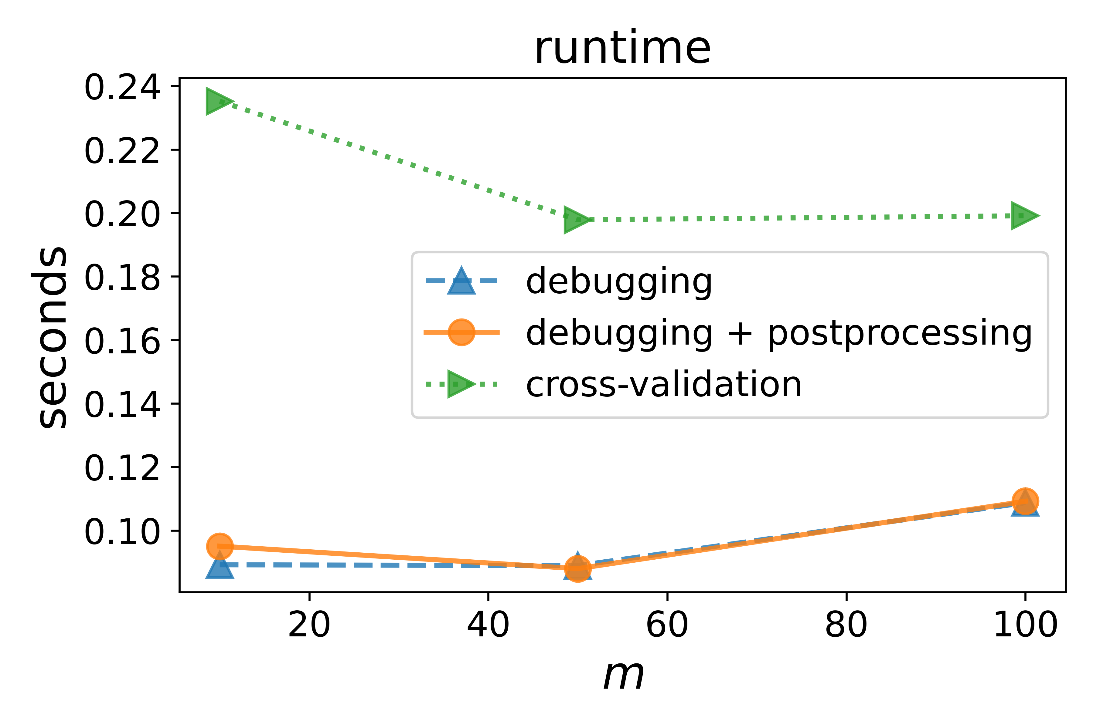
Figure 6: Effectiveness on Tuning Parameter Selection (Two Pools). Each dot is the average result of 20 random trials. We set $n=1000,p=15,t=100,L=5$, and $\sigma=0.1$.

Figure 6 displays the results for the two-pool experiments, which are qualitatively similar to the results of the one-pool experiments. We emphasize that our method works well for support recovery; furthermore, the methods exhibit comparable performance in terms of the $\ell_{2}$-error. The slightly larger error of our debugging method can be attributed to the bias which arises from using an $\ell_{1}$-norm instead of an $\ell_{0}$-norm.

6.3 Experiments with Clean Points

We now focus on debugging methods involving a second clean pool. We have three experimental designs: First, we study the influence of $m$ on support recovery. Second, we compare debugging with alternative methods suggested in the literature. Third, we study the performance of our proposed MILP debugger, where we compare it to three other simple strategies. Different strategies for selecting clean points correspond to changing step [T1] in the setup described above.

6.3.1 Number of Clean Points vs. Exact Recovery

In this subsection, we present two experiments involving synthetic and YearPredictionMSD datasets, respectively ,to see how $m$ affects the exact recovery rate. Recall that the pipeline for generating the first pool is described at the beginning of Section 6. For the second pool, we use steps [T’1, T2, T3] for the synthetic dataset, where we assume $\mathcal{P}_{X}$ is standard Gaussian. We take steps [T1-T3] for YearPredictionMSD to check the sample points in the first pool.

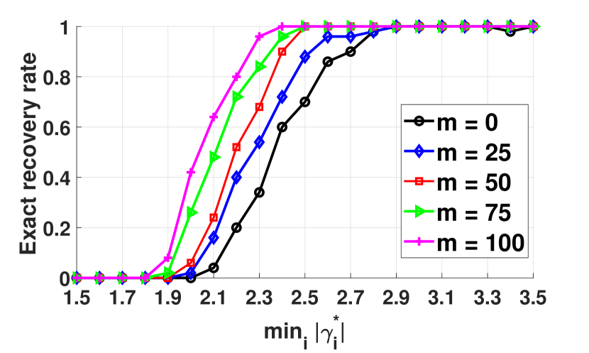
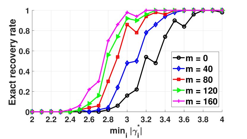
Figure 7: Minimal Gamma vs. Exact Recovery Rate on Synthetic Data. We run 50 trials for each dot and compute the average.

Recall that the YearPredictionMSD dataset is designed to predict the release year of a song from audio features. The dataset consists of 515,345 songs, each with 90 audio features. Therefore, for both experiments, we set $n=500,t=50,p=90,\sigma=0.1$, and $L=10$, and take $\lambda=2.5\frac{\sqrt{\log(n-t)}}{n}$.

From Figure 7, we see that the phenomena are similar for the two different design matrices. In particular, increasing the number of clean points helps with exact recovery. For instance, in the left subfigure, for $m=0$, when $\min_{i}|\gamma^{*}_{i}|>2.9$, the exact recovery rate goes to 1. For $m=100$, the exact recovery rate goes to 1 when $\min_{i}|\gamma^{*}_{i}|>2.4$. Also, the slope of the curve for larger $m$ is sharper. Thus, adding a second pool helps relax the gamma-min condition.

6.3.2 Comparisons to Methods with Clean Points

In this experiment, we compare the debugging method for two pools with other methods suggested by the machine learning literature. We generate synthetic data using the default first-pool setup with $n=1000,p=15,t=100$, and $\sigma=0.1$, and we run [T1-T3] to generate the second pool using different values of $m$. For our proposed debugging method, we use Algorithm 1 to select the tuning parameter. We compare the following methods: (1) debugging + postprocessing, (2) least squares, (3) simplified noisy neural network, and (4) semi-supervised eigvec. The least squares solution is applied using $\left\{\begin{pmatrix}X\\ \widetilde{X}\end{pmatrix},\begin{pmatrix}y\\ \widetilde{y}\end{pmatrix}\right\}$.

The simplified noisy neural network method borrows an idea from Veit et al. [veit2017learning], which is designed for image classification tasks for a datasets with noisy and clean points. This work introduced two kinds of networks and combines them together: the “Label Cleaning Network," used to correct the labels, and the “Image Classifier," which classifies images using CNN features as inputs and corrected labels as outputs. Each of them is associated with a loss, and the goal is to minimize the sum of the losses. Let $w\in\real,\beta_{1}\in{}^{d}$, and $\beta_{2}\in{}^{d}$ be the variables to be optimized. For our linear regression setting, we design the “Label Cleaning Network” by defining $\hat{c}_{i}=y_{i}w-x_{i}^{\top}\beta_{1}$ as the corrected labels for both noisy and clean datasets. Then we define the loss $\mathcal{L}_{clean}=\sum_{i\in cleanset}|\tilde{y}_{i}-y_{i}w-x_{i}^{\top}\beta_{1}|$. The “Image Classifier" is modified to the regression setting using predictions of $x_{i}^{\top}\beta_{2}$ and the squared loss. Therefore, the classification loss can be formalized as $\mathcal{L}_{classify}=\sum_{i\in cleanset}(x_{i}^{\top}\beta_{2}-\tilde{y}_{i})^{2}+\sum_{i\in noisyset}(x_{i}^{\top}\beta_{2}-\hat{c}_{i})$. Together, the optimization problem becomes

$$\min_{\stackrel{{\scriptstyle\beta_{1}\in{}^{d},\beta_{2}\in{}^{d}}}{{w\in\real}}}\sum_{i\in cleanset}\{(x_{i}^{\top}\beta_{2}-\tilde{y}_{i})^{2}+|\tilde{y}_{i}-wy_{i}-x_{i}^{\top}\beta_{1}|\}+\sum_{i\in noisyset}(x_{i}^{\top}\beta_{2}-wy_{i}-x_{i}^{\top}\beta_{1})^{2}.$$

We use gradient descent to do the optimization, and initialize it with $w=0$ and $\beta_{1}=\beta_{2}=\beta_{ls}$. The optimizer $\widehat{\beta}_{2}$ is used for further predictions. We then calculate $\widehat{\gamma}=y-X\widehat{\beta}_{2}$. For gradient descent, we will validate multiple step sizes and choose the one with the best performance on the squared loss of the clean pool.

The method “semi-supervised eigvec" is from Fergus et al. [fergus2009semi], and is designed for the semi-supervised classification problem. It also contains an experimental setting that involves noisy and clean data. To further apply the ideas in our linear regression setting, we make the following modifications: Define the loss function as

$$J(f)=f^{\top}Lf+\left(f-\begin{pmatrix}y\\ \tilde{y}\end{pmatrix}\right)^{\top}\Lambda\left(f-\begin{pmatrix}y\\ \tilde{y}\end{pmatrix}\right),$$

where $L=D-W(\varepsilon)$ is the graph Laplacian matrix and $\Lambda$ is a diagonal matrix whose diagonal elements are $\Lambda_{ii}=\lambda$ for clean points and $\Lambda_{ii}=\frac{\lambda}{c}$ for noisy points. In the classification setting, $f\in{}^{n+m}$ is to be optimized. The idea is to constrain the elements of $f$ by injecting smoothness/similarity using the Laplacian matrix $L$. Since we assume the linear regression model, we can further plug in $f=\begin{pmatrix}X\\ \tilde{X}\end{pmatrix}\beta$. Our goal is then to estimate $\beta$ by minimizing $J(\beta)$. As suggested in the original paper, we use the range of values $\varepsilon\in[0,1,1,5],c\in[1,10,50]$, and $\lambda\in[1,10,100]$. We will evaluate all 36 possible combinations and pick the one with the smallest squared loss on the clean pool.

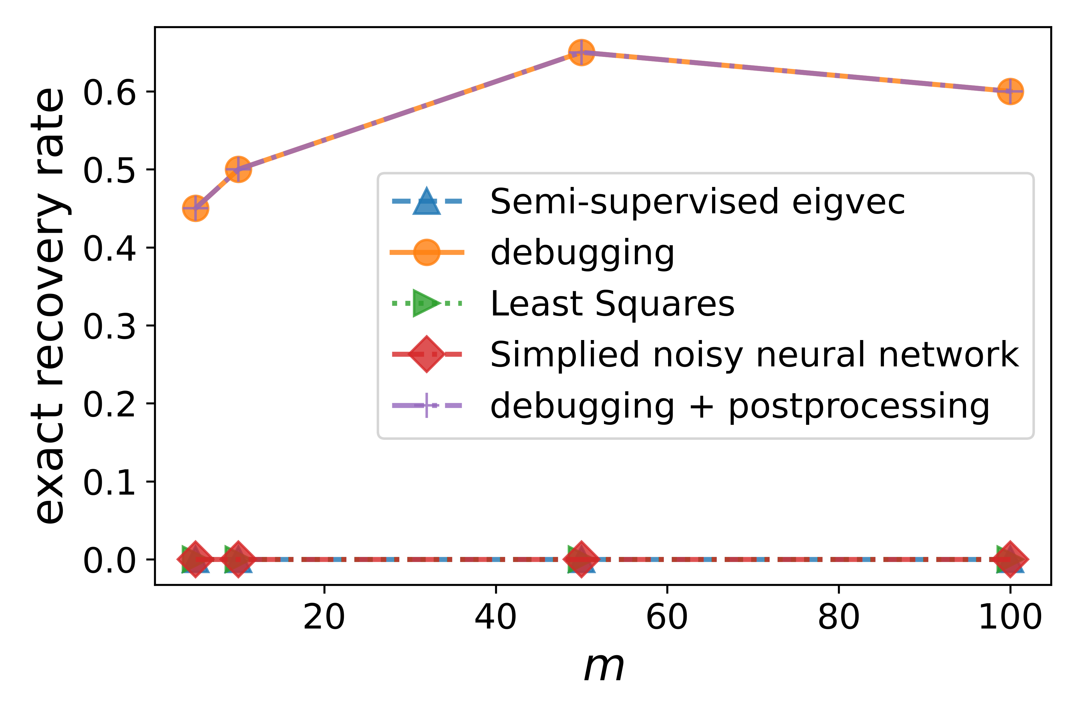
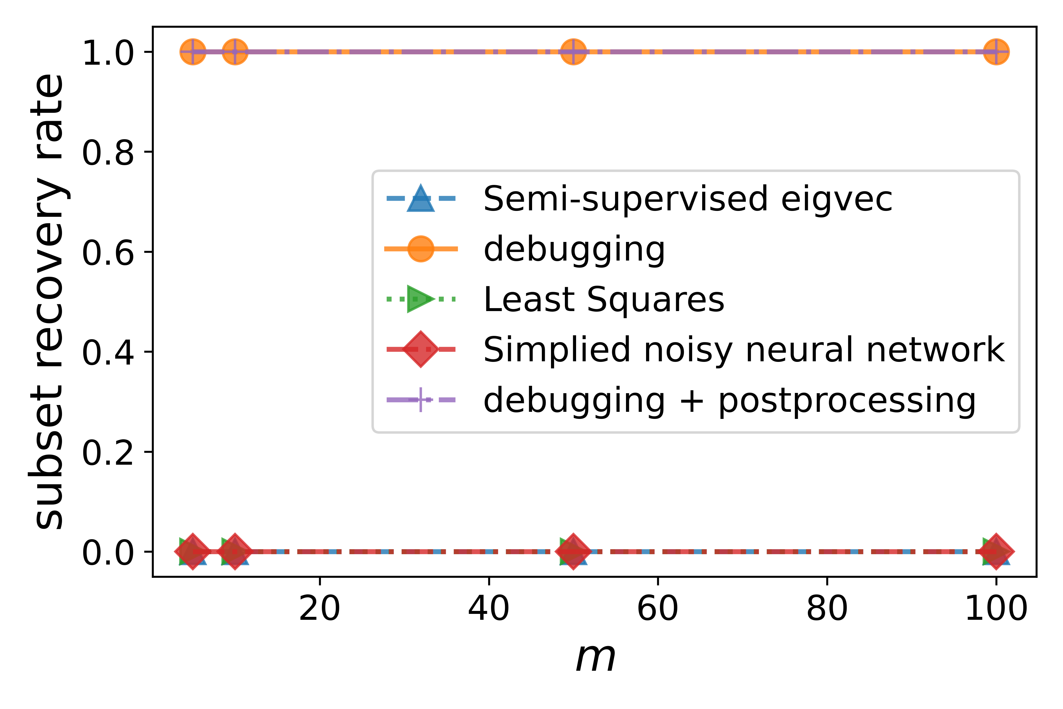
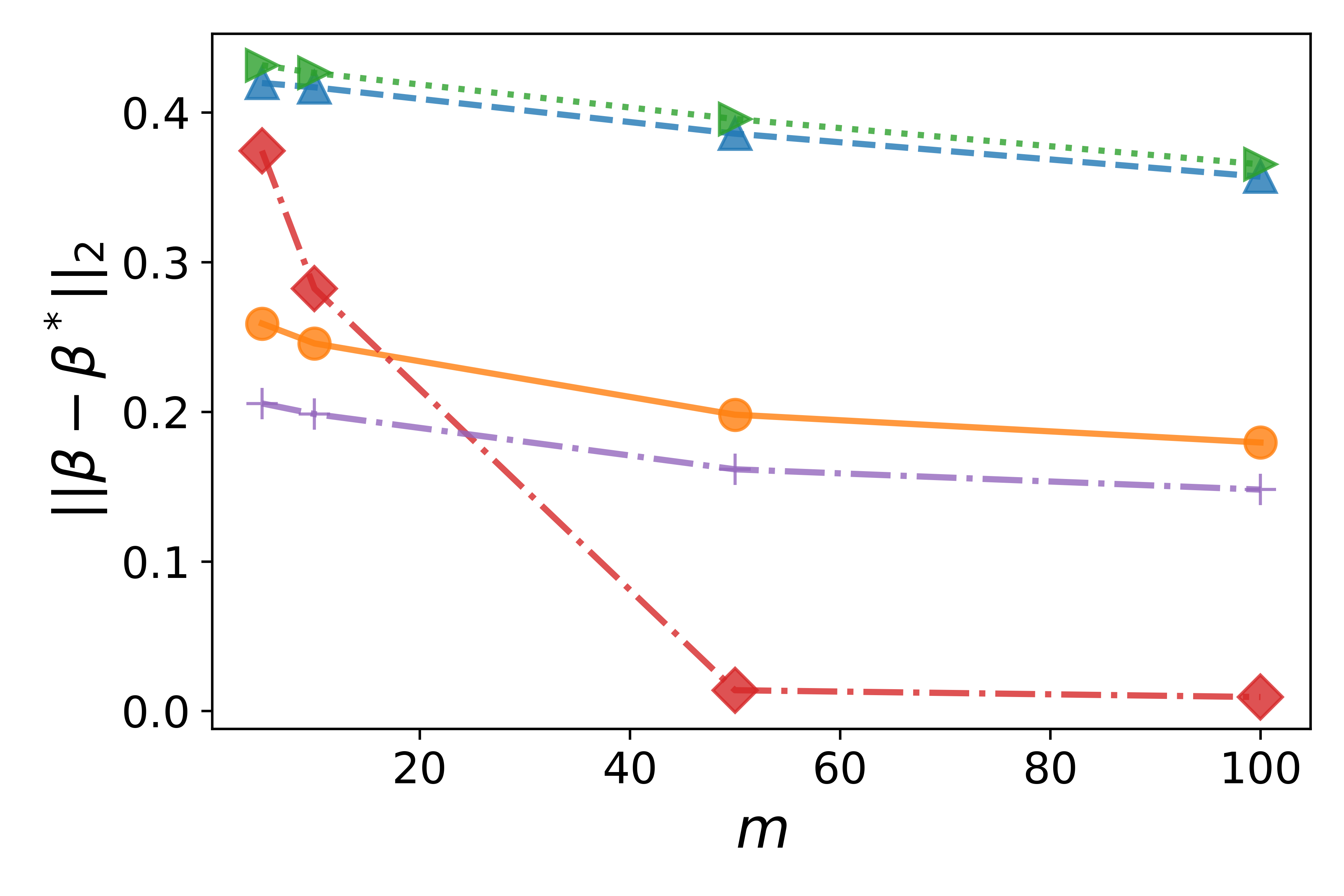
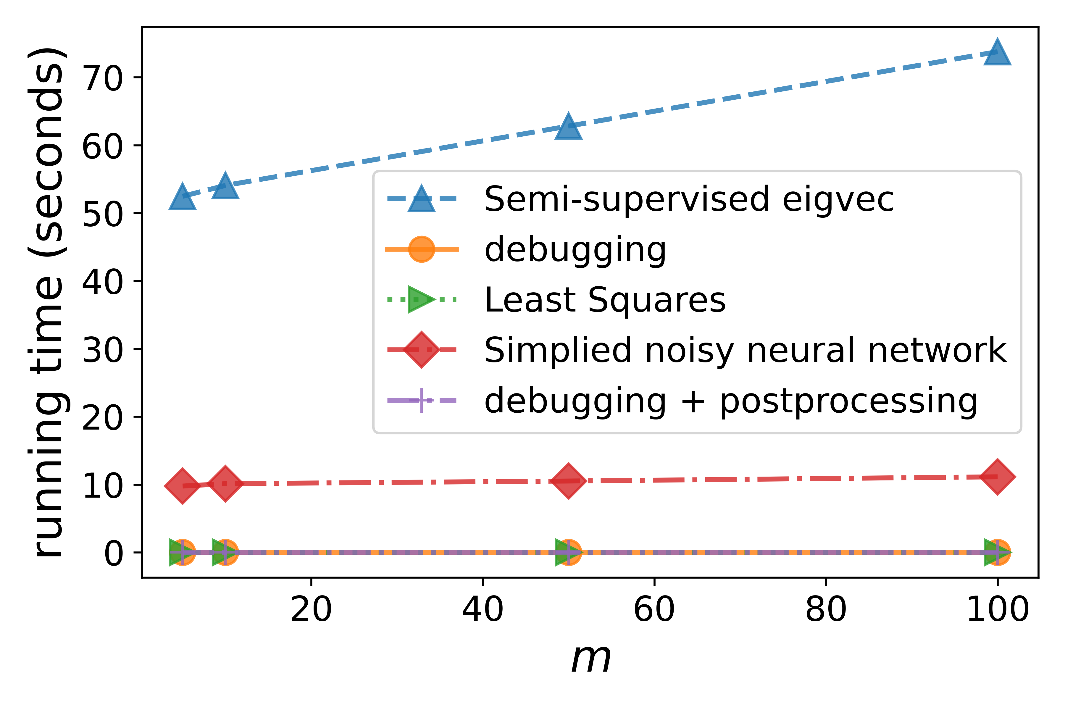
Figure 8: Comparison to Methods involving Clean Points. Each dot is the average result of 20 random trials. We use the synthetic data setting, with $n=500,p=15,\sigma=0.1,t=0.1n$, and $\min_{i}|\gamma^{*}_{i}|=10\sqrt{\log 2n}\sigma$. The clean data pool is randomly chosen from the first pool without replacement; we query the labels of these chosen points.

The results are shown in Figure 8. We observe that only the debugging method is effective for support recovery, as we have carefully designed our method for this goal. The method from Veit et al. [veit2017learning] works best in terms of $\ell_{2}$-error of $\beta$, especially when $m$ is large. The semi-supervised method, like least squares, does not perform well, possibly because it does not consider replacing/removing the influence of the noisy dataset.

6.3.3 Effectiveness on Second Pool Design

We now provide experiments to investigate the design of the clean pool, corresponding to Section 5. We use the Concrete Slump dataset, where $p=7$. We limit our study to small datasets, since the runtime of the MILP optimizer is quite long. We report the performance of the MILP debugging method in both noiseless and noisy settings. In our experiments, we compare the performance of the MILP debugger to a random debugger and a natural debugging method: adding high-leverage points into the second pool. In other words, D.milp selects $m$ clean points to query from running the MILP (18); D.leverage selects the $m$ points with the largest values of $x_{i}^{\top}(X^{\top}X)^{-1}x_{i}$; and D.random randomly chooses $m$ points from the first pool without replacement. After choosing the clean pool, the debugger applies the Lasso-based algorithm. In Zhang et al. [zhang2018training], all the second pool points are chosen either randomly or artificially. Therefore, we may consider D.random as an implementation of the method in Zhang et al. [zhang2018training], which will be compared to our D.milp.

In the noiseless setting, we define $\beta^{*}$ to be the least squares solution computed from all data points. We randomly select $n$ data points as the $x_{i}$’s. For D.milp and D.leverage, since the bug generator knows their strategies or the selected $D$, it generates bugs according to the optimization problem (17). Let $T\subseteq[n]$ be the index set of the $t$ largest $|u_{i}|$’s, for $i=1,\dots,n$. The bug generator takes $\gamma^{*}_{T}=u_{T}$ if the solution $u$ is nonzero, and otherwise randomly generates a subset $T$ of size $t$ to create $\gamma^{*}_{T}=\vec{1}$. Thus, $y_{i}=x_{i}^{\top}\beta^{*}+\gamma^{*}$. For D.onepool, the bug generator follows the above description with $D=\emptyset$. The orange bars indicate whether the bug generator succeeds in exact recovery in the one-pool case. For D.random, the bug generator generates bugs using the same mechanism as for D.onepool. Note the above bug generating methods are the “worst” in the sense of signed support recovery: The debuggers run (14) using their selected $X_{D}$. From Figure 9, there is an obvious advantage of D.milp over D.onepool and D.leverage. This suggests improved performance of our MILP algorithm. D.random is sometimes successful even when $n$ and $t$ are small because the bug generator cannot control the randomness, but it performs worse than D.milp overall.

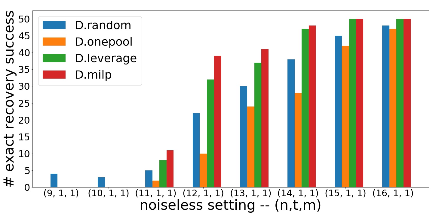
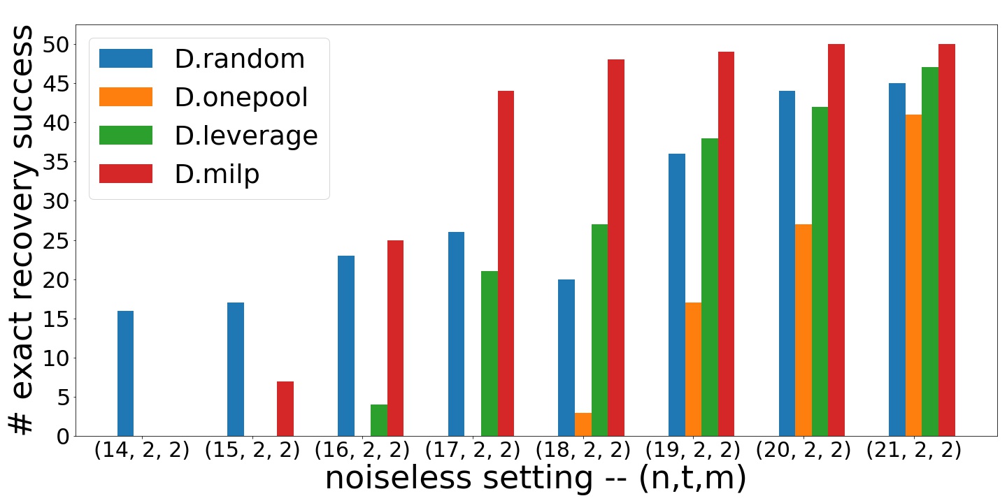
Figure 9: Comparison between D.milp and other debugging strategies in noiseless settings. Each setting is an average over 50 random trials.

In the noisy setting, we define $\beta^{*}$ to be the least squares solution computed using the entire data set. We randomly select $n$ data points as the $x_{i}$’s. For D.milp and D.leverage, since the bug generator knows their strategies or the selected $D$, it generates bugs via the optimization problem (17): taking $\gamma^{*}_{T}=u_{T}$ if the solution $u$ is nonzero for $T$ being the indices of the largest $t$ elements of $|u|$, and otherwise randomly generating a subset $T$ of size $t$ to create $\gamma^{*}_{T}=\vec{1}$. Thus, $y_{i}=x_{i}^{\top}\beta^{*}+\gamma^{*}+\mathcal{N}(0,0.01)$. Note that having $\gamma^{*}_{T}=u_{T}$ if the solution $u$ is nonzero gives incorrect signed support recovery, which is proved in Appendix LABEL:app:sign. This is related to what we have claimed in Remark 11 above. For D.onepool, the bug generator follows the above description with $D=\emptyset$. The orange bars indicate whether the bug generator succeeds in exact recovery in the one-pool case. For D.random, since it is not deterministic, the bug generator does not know $D$ and acts in the same way as in the one-pool case. Note that the above bug generating methods are the “worst” in the sense of signed support recovery. From Figure 10, there is an obvious advantage of D.milp over D.onepool and D.leverage. Our theory only guarantees the success of D.milp in the noiseless setting, so the experimental results for the noisy setting are indeed encouraging.

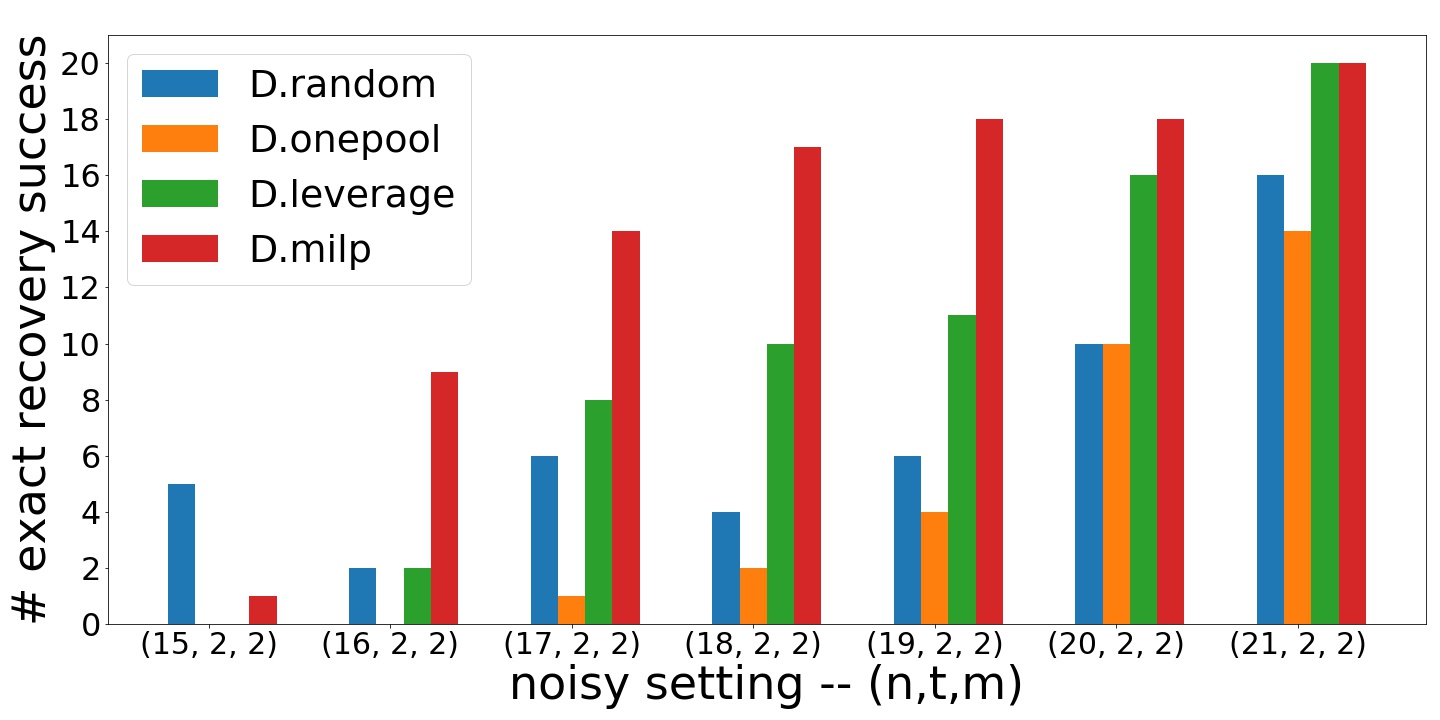
Figure 10: Comparison between MILP Strategy and Others. In each setting, we run 20 random simulations.

Debugging in practice: The algorithm for minimax optimization has been executed by running all $n\choose m$ possible choices of clean points for the outer loop; for each outer loop, we then run the inner maximization. For optimal debugging in practice, i.e., $n,t$, and $m$ being large, some recent work provides methods for efficiently solving the minimax MILP [tang2016class]. Note that the MILP debugger can be easily combined to other heuristic methods: one can run the MILP, and if there is a nonzero solution, we can follow it to add clean points. Otherwise, we can switch to other methods, such as choosing random points or high-leverage points.

7 CONCLUSION

We have developed theoretical results for machine learning debugging via $M$-estimation and discussed sufficient conditions under which support recovery may be achieved. As shown by our theoretical results and illustrative examples, a clean data pool can assist debugging. We have also designed a tuning parameter algorithm which is guaranteed to obtain exact support recovery when the design matrix satisfies a certain concentration property. Finally, we have analyzed a competitive game between the bug generator and the debugger, and analyzed a mixed integer optimization strategy for the debugger. Empirical results show the success of the tuning parameter algorithm and proposed debugging strategy.

Our work raises many interesting future directions. First, the question of how to optimally choose the weight parameter $\eta$ remains open. Second, although we have mentioned several efficient algorithms for bilevel mixed integer programming, we have not performed a thorough comparison of these algorithms for our specific problem. Third, although our MILP strategy for second pool design has been experimentally found to be effective in a noisy setting, we do not have corresponding theoretical guarantees. Fourth, our proposed debugging strategy is a one-shot method, and designing adaptive methods for choosing the second pool constitutes a fascinating research direction. Finally, the analysis of our tuning parameter algorithm suggests that a geometrically decreasing series might be used as a grid choice for more general tuning parameter selection methods, e.g., cross validation—in practice, one may not need to test candidate parameters on a large grid chosen linearly from an interval. Lastly, it would be very interesting to extend the ideas in this work to regression or classification settings where the underlying data do not follow a simple linear model.