Measuring Macroeconomic Uncertainty:
The Labor Channel of Uncertainty from a Cross-Country Perspective

This paper constructs internationally consistent measures of macroeconomic uncertainty. Our econometric framework extracts uncertainty from revisions in data obtained from standardized national accounts. Applying our model to post-WWII real-time data, we estimate macroeconomic uncertainty for 39 countries. The cross-country dimension of our uncertainty data allows us to study the impact of uncertainty shocks under different employment protection legislation. Our empirical findings suggest that the effects of uncertainty shocks are stronger and more persistent in countries with low employment protection compared to countries with high employment protection. These empirical findings are in line with a theoretical model under varying firing cost.

JEL classifications: C51, C53, C82, E32, J8

Keywords: Uncertainty Shocks, Real-Time Data, Rational Forecast Error, Employment Protection Legislation, System of National Accounts

1 Introduction

The COVID-19 crisis has highlighted the relationship between uncertainty and economic fluctuations (e.g. Altig et al. (2020)). This relationship usually differs across countries with conditions on the labor market possibly playing a decisive role. However, while theoretically important, the empirical evidence on labor market specific transmission mechanisms of uncertainty shocks on the overall economy are so far scant.

This paper proceeds in two steps. First it constructs measures of macroeconomic uncertainty that are available for a large set of countries and that are defined as the conditional volatility of an unpredictable forecast as in Jurado et al. (2015). To obtain this goal, we draw on the macroeconomic data revisions literature, thereby treating statistical agencies’ estimates of first releases of macroeconomic variables as forecasting exercises and their subsequent revisions as forecast errors. We extract the unpredictable part of data revisions by decomposing them into news – the error from an unpredictable rational forecast – and noise, which is defined as a classical errors-in-variables. Specifically, we follow the approach of Jacobs and van Norden (2011) in modeling data revisions with news and noise, enriching it with stochastic volatility components. Our measure of macroeconomic uncertainty is thus defined as the conditional volatility of the error corresponding to the unpredictable part of revisions in GDP growth. It is important to note that these estimates of macroeconomic uncertainty are consistent across OECD countries, given the nature of standardized national accounting procedures. Note also that in constructing coherent macroeconomic variables statistical agencies take into account a plethora of series that include a huge amount of sensitive data partly only available to the statistical agency. Thus, in contrast to the bottom-up approach of, e.g., Jurado et al. (2015), we follow a top-down approach, where we partly outsource the information acquisition to the statistical agency.

We apply our procedure to a post WWII real-time dataset collected for 39 countries, deriving an international set of estimates of macroeconomic uncertainty. For the U.S., our measure pinpoints periods of highest uncertainty during the mid-1970s, beginning of 1980s, beginning of 2000s, and during the recent great financial crisis, which is qualitatively consistent with other measures of U.S. uncertainty. However, our measure already peaks in the mid-1970s, highlighting the turmoils during the 1970s. We also construct a global uncertainty measure by using a GDP weighted average of all country specific uncertainty indicators. According to our measure of global uncertainty, the period during the mid-1970s and the great financial crisis stands out in terms of uncertainty, which is in line with most of the measures of global uncertainty. We also perform a VAR analysis for the U.S. and the G7 countries. The impulse response functions computed for the U.S. are very similar to impulse responses from a VAR including the uncertainty indicator of Jurado et al. (2015). These impulse response functions are qualitatively confirmed by the impulse responses estimated for an aggregate of the G7 countries.

In a second step, we use our newly created international set of indicators to investigate the role of labor adjustment costs in transmitting uncertainty shocks. We subdivide the countries into high employment protection legislation (EPL) countries and low employment protection legislation countries using the OECD Employment Protection Database. In an 8-variable VAR analysis that uses data from 1988Q1 to 2019Q4, we find that the degree of labor protection plays a crucial role in the propagation of uncertainty shocks. Uncertainty shocks affect the economy in countries with stricter employment protection legislation less than in countries with low labor protection standards. To learn more about the role played by EPL in the propagation mechanism of uncertainty shocks, we employ the theoretical model of Bloom et al. (2018). Within their framework, our focus is on the effects of changes in firing costs, assuming that stricter employment protection legislation hinders firms to lay off employees and thus lead to higher firing costs. We first calibrate, solve, and simulate the model of Bloom et al. (2018) twice, once for an economy for low EPL and once for an economy with high EPL. We then use the two calibrated models to simulate the reaction of the economy to an imposed uncertainty shock. According to the theoretical model and in line with our empirical findings, an uncertainty shock has less deteriorating effects in an economy with high EPL than in one with low EPL.

There is a rapidly expanding literature that uses forecast error based procedures to estimate uncertainty as in, e.g., Jurado et al. (2015) and Carriero et al. (2018) who employ factor stochastic volatility models to provide uncertainty measures for the U.S. Mumtaz and Theodoridis (2017), Carriero et al. (2019), Berger et al. (2017) estimate similar uncertainty indicators with a focus on extracting global uncertainty. We contribute to this literature by using real-time data on GDP growth and by computing forecast errors that incorporate information available to the economic agents up to and including at time $t$. The focus so far has only been on the last vintage of economic series at time $T$ thus incorporating information that goes beyond time $t$ with $t<T$. Limiting the construction of forecast errors to information that economic agents had about aggregate variables at time $t$ is in line with the above mentioned definition of macroeconomic uncertainty and might have important implications. Moreover, the forecast error based uncertainty literature estimates uncertainty from models that allow for changes in the underlying conditional volatility only. Drifts in the parameters of a macroeconomic model can however also stem from changes in the structure of the economy, usually modelled with time-varying coefficients. In such a setup, a model that includes stochastic volatility components only is probably misspecified. Not including time-varying coefficients possibly attributes too much variation to the stochastic volatility components, thus exaggerating the fluctuations in the uncertainty measures. We tackle this issue by allowing the coefficients of our model to change over time.

The real-time forecast errors constructed with our approach are similar to those that are computed from the survey of professional forecasters as in Jo and Sekkel (2019), Clark et al. (2020), Ozturk and Sheng (2018), and Rossi and Sekhposyan (2015). While the forecast error in our approach is constructed from the unpredictable part of revisions of GDP growth, the forecast error computed from the survey of professional forecasters are focused on single releases of GDP growth and do not incorporate revisions in GDP growth. Data revisions can thus directly affect the uncertainty measures derived from survey of professional forecasters, whereas the uncertainty indicator estimated by our procedure takes these data revisions into account. Moreover, uncertainty estimates from survey of professional forecasters are restricted to a few countries and cannot be applied to a broad-based international setting, which is the focus of this paper. There is also a literature on international uncertainty indicators that are derived from textual data. While these methods have their merits especially when it comes to real-time tracking of uncertainty, they coincide only in special cases with forecast error based uncertainty measures. Moreover, comparing uncertainty indicators from textual analysis across countries requires not only mapping the semantic meaning of words into another language but also to consider aspects of intercultural communication in order to ensure a mutual meaning of the textual analysis.

The remainder of the paper is structured as follows: In Section 2, we discuss the econometric framework and the estimation procedure. Section 3 discusses the construction of the real-time data set that serves as the basis for the uncertainty indicator. Section 4 and 5 present the uncertainty indicators and evaluate the macroeconomic relevance of uncertainty shocks. Section 6 examines the role of labor adjustment costs in the propagation of uncertainty shocks and Section 7 concludes.

2 Econometric Framework

In this section, we describe our econometric model, show how to derive direct measures of macroeconomic uncertainty, and how we cope with structural change. Finally, we briefly discuss our estimation procedure.

We follow the standard notation in the data revision literature where $y_{t}^{t+j}$ denotes an estimate published at time $t+j$ of some real-valued scalar variable $y$ at time $t$ for $t=1,...,T$ and $j=1,...,L$. According to Jacobs and van Norden (2011) the $j$th release of $y$ can be express as a function of its “true” value and a measurement error that is decomposed into a news and a noise term

$$y_{t}^{t+j}=\tilde{y}_{t}+\nu_{t}^{t+j}+\zeta_{t}^{t+j},$$ (1)

where $\tilde{y}_{t}$ represents the true value, $\nu_{t}^{t+j}$ the news component and $\zeta_{t}^{t+j}$ the noise component. Within this setup the noise component is interpreted as classical errors-in-variables and the news component as a rational forecast error. The main assumptions to distinguish between news and noise innovations are their correlation with the underlying true value of the variable. It is thus assumed that the news component carries information about the “true” value of the variable (i.e. $E[\tilde{y}_{t},\nu_{t}^{t+j}]\neq 0$), whereas the noise components are independent of the “true” value of the variable (i.e., $E[\tilde{y}_{t},\zeta_{t}^{t+j}]=0$), with $E[\nu_{t}^{t+j},\zeta_{t}^{t+j}]=0$ for all $t$ and $j$.

To estimate those news and noise components, we build on the state space model developed by Jacobs and van Norden (2011), which can be expressed as

$$Y_{t} =Z\alpha_{t},$$ (2)

$$\alpha_{t} =\varphi+T\alpha_{t-1}+R\eta_{t},$$ (3)

where

$$Y_{t}=\begin{bmatrix}y_{t}^{t+1}\\ y_{t}^{t+L}\end{bmatrix},Z =\begin{bmatrix}1&1&0&1&0\\ 1&0&1&0&1\end{bmatrix},\alpha_{t}=\begin{bmatrix}\tilde{y}_{t}\\ \nu_{t}^{t+1}\\ \nu_{t}^{t+L}\\ \zeta_{t}^{t+1}\\ \zeta_{t}^{t+L}\end{bmatrix},$$

$$\varphi=\begin{bmatrix}c\\ 0\\ 0\\ 0\\ 0\end{bmatrix},T=\begin{bmatrix}\rho&0&0&0&0\\ 0&0&0&0&0\\ 0&0&0&0&0\\ 0&0&0&0&0\\ 0&0&0&0&0\end{bmatrix},R=\begin{bmatrix}\sigma^{\nu 1}&\sigma^{\nu L}&0&0\\ 0&-\sigma^{\nu 1}&0&0\\ 0&0&0&0\\ 0&0&\sigma^{\zeta 1}&0\\ 0&0&0&\sigma^{\zeta L}\end{bmatrix},\eta_{t}=\begin{bmatrix}\eta_{t}^{\nu 1}\\ \eta_{t}^{\nu L}\\ \eta_{t}^{\zeta 1}\\ \eta_{t}^{\zeta L}\end{bmatrix}$$

with $\eta_{t}\sim N(0,I_{4})$, where $c$ and $\rho$ are coefficients and $\sigma^{i}$ represents the standard deviation of $\eta_{t}^{i}$ for $i=\nu 1,\nu L,\zeta 1,\zeta L$.

2.1 Estimating Macroeconomic Uncertainty

To obtain direct estimates of macroeconomic uncertainty, we define economic uncertainty similar to Jurado et al. (2015) as the conditional volatility of the unpredictable part of future values of the variable, i.e. in our case of subsequent releases of the variable. We thus treat the estimation procedure of early releases as a forecasting exercise. Within this context, the news components can then be seen as the unpredictable part of the forecast error. We obtain estimates of macroeconomic uncertainty by estimating changes in the variance of the news component. To do this we enrich the Jacobs and van Norden (2011) model with stochastic volatility components, modifying Equation (3) to

$$\alpha_{t} =\varphi+T\alpha_{t-1}+R_{t}\eta_{t},$$ (4)

where

$$R_{t}=\begin{bmatrix}\sigma_{t}^{\nu 1}&\sigma_{t}^{\nu L}&0&0\\ 0&-\sigma_{t}^{\nu 1}&0&0\\ 0&0&0&0\\ 0&0&\sigma_{t}^{\zeta 1}&0\\ 0&0&0&\sigma_{t}^{\zeta L}\end{bmatrix}$$

with $\sigma_{t}^{i}=\exp(h_{t}^{i})^{1/2}$ for $i=\nu 1,\nu L,\zeta 1,\zeta L$ and $\alpha_{t}$, $\varphi$, $T$ and $\eta_{t}$ specified as in (3). The volatility components are modelled as latent variables whose logarithms are assumed to follow independent AR(1) processes:

$$h_{t}^{i}=\mu^{i}+\phi^{i}(h_{t-1}^{i}-\mu^{i})+\tau^{i}\epsilon_{t}^{i},$$ (5)

where $\mu^{i}$, $\phi^{i}$, $\tau^{i}$ are parameters, $\epsilon_{t}^{i}\sim N(0,1)$ and $i=\nu 1,\nu L,\zeta 1,\zeta L$.

Our measure of macroeconomic uncertainty at time $t$ can thus be expressed as

$$U_{t}\equiv\sigma_{t}^{\nu 1}+\sigma_{t}^{\nu L},$$

which is a combination of the conditional volatility of the two rational forecast errors.

2.2 Capturing Structural Change

In dynamical systems of macroeconomic developments variations in the underlying volatility are intertwined with changes in the structure of the economy, i.e. time-varying coefficients. If drifts in the system are characterized by structural changes in the economy, a model that includes stochastic volatility components only is possibly misspecified. In such a setup, not allowing for time-varying coefficients would possibly attribute too much time-variation to the stochastic volatility components, exaggerating the time variation in the stochastic volatility components.

In our setup, we model structural changes as variations in the stochastic properties of the “true” value $\tilde{y}_{t}$. We capture this change by allowing the coefficients in the equation of $\tilde{y}_{t}$ to vary over time, modifying Equation (4) to:

$$\alpha_{t} =\varphi_{t}+T_{t}\alpha_{t-1}+R_{t}\eta_{t},$$ (6)

where

$$\varphi_{t}=\begin{bmatrix}c_{t}\\ 0\\ 0\\ 0\\ 0\end{bmatrix},T_{t}=\begin{bmatrix}\rho_{t}&0&0&0&0\\ 0&0&0&0&0\\ 0&0&0&0&0\\ 0&0&0&0&0\\ 0&0&0&0&0\end{bmatrix}$$ (7)

and

$$\begin{bmatrix}c_{t}\\ \rho_{t}\end{bmatrix} =\begin{bmatrix}c_{t-1}\\ \rho_{t-1}\end{bmatrix}+\begin{bmatrix}\epsilon_{t}^{c}\\ \epsilon_{t}^{\rho},\end{bmatrix}$$

with $[\epsilon_{t}^{c}\ \epsilon_{t}^{\rho}]^{\prime}\sim N(0,V)$ and $\alpha_{t}$, $R_{t}$ and $\eta_{t}$ specified as in (4).

2.3 Priors

We use priors that are as diffuse as possible. The prior on $V$ is assumed to follow an Inverse Wishart distribution. The shape parameter is set to 3. The prior for the scale parameter is optimized according to the length of the series, in order for the AR(1) to cover the range of possible values. The prior for the variance of the stochastic volatilities is assumed to follow an Inverse Gamma distribution. We set the priors on the variance of the stochastic volatilities as uninformative as possible.

2.4 Estimation Procedure

We obtain draws from the posterior of our model’s parameters using Markov Chain Monte Carlo methods. More specifically, we use Gibbs sampling. The Gibbs sampler consists of the following blocks:

1. Draw $\alpha_{t}$ conditional on $\varphi_{t}$, $T_{t}$, $R_{t}$ and data $Y_{t}$ using a forward filtering backward sampling as described in, e.g., Carter and Kohn (1994),

2. Draw $h_{t}^{i}$, $\mu^{i}$, $\phi^{i}$, $\tau^{i}$ for $i=\nu 1,\nu L,\zeta 1,\zeta L$ conditional on $\alpha_{t}$, $\varphi_{t}$, $T_{t}$ using the ancillarity-sufficiency interweaving approach proposed by Kastner and Frühwirth-Schnatter (2014),

3. Draw $\varphi_{t}$ and $T_{t}$ conditional on $\alpha_{t}$ and $R_{t}$ using the simulation smoothing approach introduced by McCausland et al. (2011).

4. Draw $V$ conditional on $\alpha_{t}$, $R_{t}$, $\varphi_{t}$ $T_{t}$ from an Inverse Wishart distribution.

See Appendix A for a more detailed discussion of our estimation procedure.

3 Real-Time Data

We use data revisions in real GDP growth for 39 countries to construct the uncertainty indicator. Particularly, we use the first year-over-year growth rate of real GDP as a forecast for the final year-over-year growth rate of real GDP that we define as the growth rate published after three years. In order to obtain a comprehensive data set for various countries, we need to tap and combine several data sources. The largest part of our data is provided by the Original Release Data and Revisions Database. The Original Release Data and Revisions Database is part of OECD Main Economic Indicators database (OECD, 2017) and represents the central data source of this project. The database provides different releases of macroeconomic aggregates for many countries. This study uses data from 39 countries. Table 1 provides an overview of the countries included in our study, the data provider and the first available data point. Unfortunately, the Original Release Data and Revisions Database provides releases of macroeconomic variables only since 1999. For data prior to 1999, we need to rely on other data sources. We primarily use the data made available by the Federal Reserve Bank of Dallas for releases prior to 1999. Fernandez et al. (2011) collect real-time data for various economies including those that we use in this study. The authors assemble the dataset from original quarterly releases of different macroeconomic aggregates from 1962 to 1998. We currently use these data for all countries except the U.S., Germany, Italy, Australia and New Zealand. For the U.S., we use data provided by the Federal Reserve of Philadelphia as they provide more exhaustive data compared to the data provided by Federal Reserve of Dallas. For Germany we rely on data provided by Boysen-Hogrefe and Neuwirth (2012) and for Australia we use data provided by the Australian Real-Time Macroeconomic Database (Lee et al., 2012). For New Zealand we use data provided by the Reserve Bank of New Zealand (Sleeman, 2006) and for Italy, we also use data releases of ISTAT that were kindly provided by Golinelli and Parigi (2008).

Table 1: Data Source of Uncertainty Indicators

Countries	MEI Code	Datasource prior to 1999	Available since
Australia	AUS	Real-Time Macroeconomic Database (U. Melbourne)	1967 Q3
Austria	AUT	FED Dallas	1999 Q3
Belgium	BEL	no data	1999 Q1
Brazil	BRA	no data	2000 Q2
Canada	CAN	FED Dallas & Bank of Canada	1961 Q3
Chile	CHL	no data	2010 Q1
Czech Republic	CZE	no data	1999 Q1
Denmark	DNK	FED Dallas	1993 Q2
Estonia	EST	no data	2010 Q3
Finland	FIN	FED Dallas	1993 Q4
France	FRA	FED Dallas	1987 Q2
Germany	DEU	FED Dallas & Boysen-Hogrefe and Neuwirth (2012)	1964 Q4
Great Britain	GBR	FED Dallas	1964 Q4
Hungary	HUN	no data	2002 Q2
Greece	GRC	no data	2003 Q4
Iceland	ISL	no data	2002 Q4
India	IND	no data	2005 Q4
Indonesia	IDN	no data	2005 Q4
Ireland	IRL	no data	2002 Q2
Israel	ISR	no data	2010 Q2
Italy	ITA	FED Dallas & Golinelli and Parigi (2008)	1974 Q3
Japan	JPN	FED Dallas	1964 Q3
Korea	KOR	FED Dallas	1996 Q4
Luxembourg	LUX	no data	2004 Q4
Mexico	MEX	FED Dallas	1994 Q2
Netherlands	NLD	FED Dallas	1993 Q3
New Zealand	NZL	Reserve Bank of New Zealand	1994 Q4
Norway	NOR	FED Dallas	1993 Q3
Poland	POL	no data	2002 Q2
Portugal	PRT	FED Dallas	1992 Q3
Russia	RUS	no data	1999 Q3
Slovakia	SVK	no data	2000 Q3
Slovenia	SVN	no data	2010 Q1
South Africa	RUS	no data	2001 Q4
Spain	ESP	FED Dallas	1993 Q1
Sweden	SWE	FED Dallas	1989 Q4
Switzerland	CHE	FED Dallas	1987 Q2
Turkey	TUR	FED Dallas	1993 Q1
USA	USA	FED Philadelphia	1961 Q4

Notes: Central data source is the Original Release Data and Revisions Database. The column Countries depicts the country and MEI Code the country code from the Original Release Data and Revisions Database. The column Datasource prior to 1999 describes the data source of releases prior to 1999. The column Available since states beginning of a country’s uncertainty indicator. Rows in green highlight countries with data available prior to 1990Q1, rows in gray depict countries with data from 1990Q1 to 2000Q4 and rows in red represent countries with data available only from 2001Q1 onward.

While data availability fluctuates a lot between countries, we have surprisingly long time series for many countries. For 10 countries we have real-time data for more than 30 years (green shaded countries) and for another 16 countries we have more than 20 years of data (gray shaded countries). For four countries only, we have less than 10 years data. Besides data availability, also the average revisions change heavily between single countries. While large countries in terms of GDP, such as the U.S., France, Germany, Canada and Australia tend to have small revisions, smaller countries, including Ireland, Island and Luxembourg, appear to have much larger revisions. Figure 1 visualizes the distribution of the 10th revision of year-over-year growth rates of real GDP for different countries.

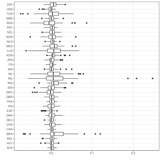
Figure 1: Boxplot of the 10th revision of real GDP growth for the periods from 2000 Q1 onward.

Most countries reveal a statistical significant upward revision of their growth rates over time. The 10th release of GDP growth tends on average to be larger than the first release. Only four countries including the U.S., Russia, Greece and Spain, report on average a lower growth rate at the 10th release than on the first release.

4 Estimates of Macroeconomic Uncertainty

Using the econometric framework outlined in Section 2 and the real-time dataset described in Section 3, we obtain estimates of macroeconomic uncertainty for 39 countries. We now present and discuss the resulting uncertainty measures. Thereby, we focus on uncertainty in the United States and global uncertainty.

Our methodical framework provides macroeconomic uncertainty estimates for the United States that are similar to existing uncertainty measures. Figure 2 presents our revision-based uncertainty measure for the U.S. (blue solid line) and compares it to existing proxies found in the literature. These alternative measures include the macroeconomic uncertainty indicator proposed by Jurado et al. (2015) (green solid line), the economic policy uncertainty index developed by Baker et al. (2016) (ochre dashed line) and the VIX (purple dashed line), a popular uncertainty indicator that reflects market’s expectation of volatility implied by the S&P 500 index options.

Figure 2: Uncertainty United States: Macroeconomic Uncertainty
Notes: This figure compares different uncertainty indicators for the United States form 1960Q1 to 2019Q4. In the first pane, the green solid line displays the indicator for macroeconomic uncertainty (quarterly averages, horizon 12, MacroFinanceRealUncertainty_202008_update) developed by Jurado et al. (2015) and the blue solid line shows the newly proposed measure of macroeconomic uncertainty. In the second pane, the dashed ochre line shows quarterly average of the Economic Policy Indicator proposed by Baker et al. (2016). The last pane compares the VIX (realisied volatility before 1989) to the new uncertainty measure. All indicators are demeaned and normalized to unit variance.

Our data revision based indicator reaches its highest levels during the recession in the 70s that was characterized by the first oil price shock and the collapse of the Bretton Woods system and marked the end to the overall Post-World War II economic expansion. The Great Recession of 2008 represents the second highest peak of our uncertainty measure. Further identified times of heighten uncertainty are during the ’82 recession and, to a much lesser extent, at the beginning of the 2000s, during the dotcom bubble burst. Overall, our indicator resembles most the uncertainty measure proposed by Jurado et al. (2015)(henceforth JLN). However, while JLN peaks during the Iran Revolution in 1979, the revision based indicator reaches its highest levels during the 70s recession. Compared to other uncertainty measures, our uncertainty estimate for the U.S. displays a significantly lower volatility and indicates only a few mayor uncertainty shocks during 1965 and 2019. For instance, while both the EPU and the VIX peak in 1987 as a result of the Black Monday, the revision based indicators hardly blinks. Similar, after the Great Recession of 2008, the EPU reaches all-time-high level of economic policy uncertainty. However, the economic policy uncertainty does not translate into macroeconomic uncertainty as both the revision based indicator as well as JLN return to very low levels after the recession.

Although we obtain uncertainty estimates for 39 countries, for the sake of brevity, we abstain from discussing all countries in the main text and refer the reader to Appendix C for a presentation of all uncertainty indicators. Instead, we use the comprehensive number of uncertainty indicators to examine uncertainty on a global level. We construct a global uncertainty measure as the weighted mean of single country indicators. We achieve this by first standardizing the uncertainty indicator of each country and then computing the weighted average by weighing each country according to its real GDP. The countries included in the construction of the global uncertainty indicator account for approximately 50% of world GDP during the first half of the sample. During the second half of the sample, the included countries account for more than 75% of world GDP. Figure 3 presents the global uncertainty indicators. From the 1960s to today, our estimates suggest two large global uncertainty shocks. The first occurred during the oil price shock in the 70s, the second global uncertainty shock was experienced during the Great Recession in 2008. The only other notable increase in global uncertainty occurred after the second oil price shock and the subsequent early 80s recession.

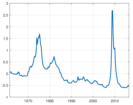
Figure 3: Global Uncertainty

Notes: This figure shows the weighted average of countries’ normalized uncertainty measures. We weight single countries according to their real GDP. While the included countries represent approximately half of world GDP during the first half of the sample, the economies included in the second half represent around 75% of total GDP.

Recently, various papers started to measure and study uncertainty on a global dimension. While several papers propose measures of global economic policy uncertainty, world risk and global financial uncertainty, studies that attempt to measure global macroeconomic uncertainty are limited: Redl (2017) constructs a JLN based global uncertainty measure that uses global macro and financial data from emerging and advanced economies. Mumtaz and Theodoridis (2017) (henceforth MT) use a factor model with stochastic volatility to decompose the time-varying variance of macroeconomic and financial variables of eleven OECD countries into contributions from country-specific uncertainty and uncertainty common to all countries. Carriero et al. (2019) (henceforth CCM) estimate a large, heteroskedastic VAR on 19 industrialized economies to obtain estimates of global uncertainty. Berger et al. (2017) (henceforth BGK) use a dynamic factor model with stochastic volatility to identify the common component of macroeconomic uncertainty from 20 OECD countries. Figure 4 compares these indicators to our data-revision based indicator. While the data revision based indicator matches the other indicators remarkably well, two differences stand out. First, similar to the indicator of the U.S., the data revision based indicator is the least volatile of all indicators. Second, while the other four indicators peak during the great recession of 2008 at 4 standard deviations or higher above their mean, the data revision indicator peaks at 2.5 standard deviations.

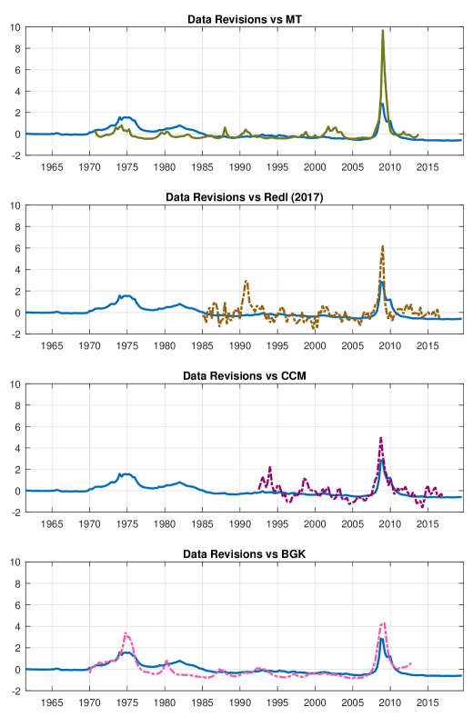
Figure 4: Global Macroeconomic Uncertainty
Notes: This figure compares different global macroeconomic uncertainty indicators. In the first pane, the green solid line displays the indicator for global macroeconomic uncertainty by Mumtaz and Theodoridis (2017) and the blue solid line shows the data revision based indicator of global macroeconomic uncertainty. In the second pane, the dashed ochre line shows quarterly averages of the global macroeconomic uncertainty measure proposed by Redl (2018). The third pane compares the global uncertainty indicator by Carriero et al. (2019) to the new uncertainty measure. The last pane display the indicator proposed by Berger et al. (2017) together with the revision based indicator. All indicators are demeaned and normalized to unit variance.

5 Cross-Country Impact of Uncertainty Shocks

Following the existing empirical research on uncertainty, we use a VAR analysis to study the dynamic relationships between macroeconomic activity and uncertainty. We consider the following VAR model:

$$x_{t}=c_{b}+B_{1}x_{t-1}+B_{2}x_{t-2}+...+B_{p}x_{t-p}+u_{t},$$ (8)

where $x_{t}$ is a $n\times 1$ vector containing all $n$ endogenous variables, $t=1,...,T$ denotes time, $c_{b}$ is a $n\times 1$ vector of constants, $B_{i}$ for $i=1,...,p$ are $n\times n$ parameter matrices and $u_{t}$ is the $n\times 1$ one-step ahead prediction error with $u_{t}\sim N(0,\Sigma)$, where $\Sigma$ is the $n\times n$ variance-covariance matrix. The prediction error $u_{t}$ can be written as a linear combination of structural innovations $u_{t}=A\epsilon_{t}$ with $\epsilon_{t}\sim N(0,I_{n})$, where $I_{n}$ is an $(n\times n)$ identity matrix and where $A$ is a non-singular parameter matrix.

We choose a recursive identification scheme and a VAR similar to the one proposed in Basu and Bundick (2017), augmenting their VAR setup with a stock market index. Similar to Bloom (2009), we include the stock-market level as the first variable in the VAR. We order uncertainty last to make sure that the impact of all other shocks is already considered for when evaluating the impact of uncertainty on the economy. The ordering of our VAR is as follows:

$$\begin{bmatrix}\textit{stock market}\\ \textit{policy rate}\\ CPI\\ employment\\ investment\\ consumption\\ GDP\\ uncertainty\end{bmatrix}.$$ (9)

We estimate the model using Bayesian methods, specifying diffuse priors. Similar to Jurado et al. (2015), we use the posterior mean of our uncertainty indicator discussed in the Section 4 as a measure for macroeconomic uncertainty in our VAR. However, as a further robustness check, we have also estimated the VAR taking into account the uncertainty surrounding our uncertainty indicator. To incorporate the whole posterior distribution instead of just the posterior mean, we extend the algorithm in Section 2.4 by one further block. In this additional step, we obtain a draw for the VAR parameters from a Normal-Inverse Wishart distribution, conditional a draw simulated from the posterior of the uncertainty indicator. The resulting posterior distributions are summarized in Figures 14 and 15 in Appendix E.

5.1 Impact of Uncertainty Shock in the U.S.

We employ the described VAR to investigate the impulse responses functions of key macro variables to uncertainty shocks that are derived using our data revision based uncertainty measure. To validate our uncertainty measure, we compare the impulse responses obtained using the data revisions based uncertainty measure to impulse response functions that are computed with the macroeconomic uncertainty index by Jurado et al. (2015). The estimation sample spans the period 1982Q1–2019Q4.

Figure 5 reports the impulse responses of GDP, investment, employment and consumption to an uncertainty shock in the United States. A one standard deviation shock in uncertainty has an adverse and enduring effect on all macroeconomic variables (blue dashed line). For most of the variables the drop lasts for about two years, with most of posterior probability mass lying below zero. During this period output declines by around 0.4%, investment by 1% and, employment and consumption by about 0.5%. The recovery from the uncertainty shock takes up to 10 years and more. While these effects seems somewhat strong and long-lasting, they are very similar to the uncertainty measure of Jurado et al. (2015) (green line).

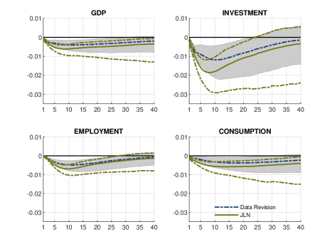
Figure 5: Impulse responses to an uncertainty shock in the U.S.

Notes: The dotted blue line depicts the posterior mean and the grey shaded area the 68% error bands for the impulse responses to an one standard deviation uncertainty shock computed from a VAR model including the uncertainty measure based on data revisions. The solid green line depicts the posterior mean with the dotted green lines representing the 68% error bands for the impulse responses from a model that uses the uncertainty measure of Jurado et al. (2015). The estimation sample spans the period 1982Q1–2019Q4.

5.2 Impact of Uncertainty Shock in G7 countries

In this section, we examine the effects of uncertainty shocks within an international context. Thereby, we use a subset of the uncertainty indicators discussed in Section 4 to estimate the VAR model outlined above for the G7 countries. The intergovernmental economic organization comprises Canada, France, Germany, Italy, Japan, United Kingdom and the United States. In terms of economic importance, the organization makes up for about one third of global GDP based on purchasing power parity. Due to data limitations, we confine our estimates the sample from 1988Q1 to 2019Q4 for all countries. We employ the following country-specific VAR model

$$x_{i,t}=c_{i,b}+B_{i,1}x_{i,t-1}+B_{i,2}x_{i,t-2}+...+B_{i,p}x_{i,t-p}+u_{i,t},$$ (10)

where $x_{i,t}$ is a $n\times 1$ country-specific vector containing all $n$ endogenous variables for country $i=1,...,N$ and time $t=1,...,T$. $c_{i,b}$ is an $n\times 1$ country specific fixed effect, $B_{1},B_{2}...,B_{p}$ are $n\times n$ parameter matrices and $u_{i,t}$ is the $n\times 1$ disturbance with $u_{i,t}\sim N(0,\Sigma_{i})$, where $\Sigma_{i}$ is the $n\times n$ variance-covariance matrix. To obtain an aggregate impulse response for the G7 countries we average across country-specific impulse responses.

Figure 6 shows the cross-country average impulse responses of GDP, investment, employment and consumption to an uncertainty shock. All variables unveil a negative relationship with uncertainty. While the impulse responses for the G7 aggregate in Figure 6 are qualitatively similar to the impulse responses obtained for the United States reported in Figure 5, the average G7 effect of uncertainty shock is about half as strong as the one found for the United States.

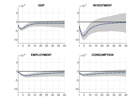
Figure 6: Impulse responses to an uncertainty shock for the group of G7 countries

Notes: The dotted blue line depicts the posterior mean and the grey shaded area the 68% error bands for the impulse responses to an one standard deviation uncertainty shock. The estimation sample spans the period 1988Q1–2019Q4.

6 On the Role of Employment Protection Legislation

Various studies have documented the negative impacts of uncertainty shocks on the labor market. However, while the importance of the investment channel for the propagation of uncertainty shocks has been extensively studied in the literature, fewer studies focus on labor markets rigidities as the dominant transmission channel of uncertainty to the real economy. Recently, however, scholars started to explore this channel in more detail. Cacciatore and Ravenna (2015), for instance, show that binding downward rigidity of wages reinforce the negative effects of uncertainty on employment. In a similar fashion, Leduc and Liu (2016) claim that nominal rigidities amplify the option-value channel through which uncertainty transmits the economy. Guglielminetti (2016) shows that firms reduce open vacancies when uncertainty increases in order to avoid expensive search activities and highlights its importance for the transmission of uncertainty shocks. Matute and Amann (2018), Riegler (2014) and Jo and Lee (2019) study the impact of uncertainty shock on labor flows. Summarizing, the authors find that uncertainty reduces hiring and increases lay offs and voluntary quits. In this study, we focus on the role of firing costs as a possible transmission mechanism of uncertainty shocks. We proxy firing costs with the degree of employment protection legislation and argue that stricter employment protection makes it more difficult—and thus more costly—to fire employees.

To obtain a better understanding of the role of employment protection legislation (EPL) in the propagation of uncertainty shocks, we first study the role of EPL within a theoretical framework and, in a second step, we use our newly developed uncertainty measures to empirically test the theoretical predictions.

6.1 Theoretical Model

To study the importance of EPL for uncertainty shocks within a theoretical model, we need a model that features uncertainty shocks and allows us to impose a stricter EPL. The dynamic stochastic general equilibrium model proposed by Bloom et al. (2018) includes these necessary features. The real business cycle model considers an economy with identical households wanting to maximize life-time discounted utility. All households choose how much they want to consume, work, and invest in order to maximize their life-time utilities. Furthermore, the model features an economy with heterogeneous firms that use labor and capital to produce a final good with the objective to maximize the life-time discounted value of their firm. Firms are subject to an exogenous process of productivity that has a firm-level and a macroeconomic component. Both the macroeconomic as well as the idiosyncratic productivity process vary in the first and second moment, with changes in second moment representing changes in uncertainty. Firms react to changes in productivity by adjusting capital and labor. However, adjusting capital and labor comes at a cost that firms have to take into account when maximizing their firm value.

We chose the model by Bloom et al. (2018) because of the exhaustive way to simultaneously model capital and labor adjustment costs. In our case, we are particularly interested in the way the authors model labor adjustment costs. The model includes two types of labor adjustment costs ($AC^{n}$). Firms face fixed and linear costs when adjusting labor. Fixed costs represent a lump sum cost that arises when employees are hired or fired. This cost does not depend on the size of the adjustment but on the state of the economy. One can think of these costs as arising from the deficiency in production owing to an experienced employee leaving the company or a new employee entering it. In contrast to fixed costs, linear costs depend on the size of the labor adjustment. These costs include, among others, recruiting and training costs for new employees and severance payment when laying off employees. Labor adjustment costs can thus be formally expressed as

$$AC^{n}=\mathbbm{1}(|s|>0)y(z,A,k,n)C^{F}_{L}+\mathbbm{1}(s>0)C^{P}_{H}w+\mathbbm{1}(s<0)C^{P}_{F}w,$$ (11)

where $C^{F}_{L}$ represent fixed labor adjustment costs that depend on the current state of production $y(z,A,k,n)$. $\mathbbm{1}(\cdot)$ represents an indicator function and $s$ indicates the change in employment. $C^{P}_{H}$ and $C^{P}_{F}$ represent hiring and firing costs as a percentage of the annual wage bill $w$.

As we aim to examine the effects of stricter employment protection legislation, we adjust the parameter that we associate most with stronger labor protection: firing costs. Stricter employment protection legislation makes it harder for firms to lay off employees. Hence, stricter employment protection legislation increases firing costs. Theoretically, firing costs change the effects of uncertainty on employment in two ways. First, an increase in firing costs reduces firing when uncertainty increases. Second, an increase in firing costs reduces hiring. The reason for this is the following: In the presence of non-convex adjustment costs—firing costs in our case—firms face Ss hiring/firing policy rules (Scarf, 1959). That is, firms do not hire new employees until productivity reaches an upper threshold (the S in Ss) and do not fire employees until its productivity hits a lower threshold (the s in Ss). Stricter employment protection legislation reduces the lower threshold. Hence, productivity needs to fall more before firms start firing employees. Overall employment will fall less compared to an economy with lower employment protection standards. This mechanism is similar to the one described by Bell (2016). Using a partial equilibrium model, the author shows that an increase in firing costs has a negative effect on employment because firms reduce hiring due to precautionary reasons. Overall, however, the negative effect on uncertainty is reversed as the increase in costs discourages firing by more than it does hiring. The reason being that laying off employees causes immediate costs, while hiring costs are discounted as they only become relevant once a firm fills the vacant position again.

In order to study the role of EPL the propagation of uncertainty shocks we calibrate, solve and simulate the model of Bloom et al. (2018) twice, once for an economy for low EPL and once for an economy with high EPL. In order to ensure comparability with Bloom et al. (2018) and the RBC literature in general, we do not change the calibration proposed by Bloom et al. (2018), except for the firing cost parameter. For the United States, Bloom et al. (2018) assume firing costs to be on average 1.8% of an annual wage bill. For continental European economies—countries that according to the OECD Employment Protection Database have on average stricter EPL—studies report substantially higher firing costs (Grund, 2006, Kramarz and Michaud, 2010). It is surprisingly hard to find studies quantifying firing costs for countries other than the US. Del Boca and Rota (1998) interview Italian manufacturing firms and find firing costs that range from less than half a monthly (3.6% of an annual wage bill) of labour cost to up to 20 months of labour costs (166% of an annual wage bill) in cases of a conflict. Unfortunately, the authors do not provide averages. For illustrative purposes, we start from the lowest reported value that is twice as high as in the case of Bloom et al. (2018), i.e. we assume firing costs to be on average 3.6% of an annual wage bill. Table 2 summarizes the labor adjustment parameters.

Parameter Description		Low EPL	High EPL
$C^{F}_{L}$:	fixed hiring/firing costs (% sales)	0.021	0.021
$C^{P}_{H}$:	per capita hiring (% of annual wage bill)	0.018	0.018
$C^{P}_{F}$:	per capita firing cost (% of annual wage bill)	0.018	0.036

Table 2: Model Calibration

Notes: This table presents the model calibration and parameter choices. The calibration reflects a quarterly calibration of the model and is based on Bloom et al. (2018).

We use two differently calibrated models to simulate the reaction of the economy to an uncertainty shock. In the case of this model, an uncertainty shock corresponds to an increase in variance of the shock distribution from which future realisations of productivity (TFP) will be drawn. Figure 7 presents the impulse responses of output, investment, employment and consumption to an uncertainty shock. The blue lines presents the impulse response of an uncertainty shock under low employment protection legislation and the gray line shows the impulse response of the same uncertainty shock under high employment protection. Both economies contract after an uncertainty shock. The uncertainty shock causes an immediate contraction of output in the first period followed by a recovery starting in the subsequent quarters. Three channels contribute to this fall in output: the investment channel, the employment channel, and the misallocation of factors of production. The presence of capital adjustment costs causes investment to drop sharply after an uncertainty shock. In the first period investment drops by around 15% followed by a rapid recovery. Also employment reacts negatively to an uncertainty shocks. As firms face firing and hiring costs when adjusting their number of employees, an increase in uncertainty reduces hiring and firing activities of firms. Thereby, hiring decreases more than firing. Moreover, employment also decreases because of labor attrition. Finally, the decrease in firing and hiring increases the misallocation of factors of production. Households expect the increase in misallocation to decrease future productivity and thus to lower the expected return on savings making immediate consumption more attractive. These dynamics lead in combination with the available resources in the economy—the capital stock does not adjust to uncertainty in period one—to an increase in consumption in the first period. The increase of consumption following an uncertainty is a well-known artefact of this model. Bloom et al. (2018) extensively discuss this behaviour in their paper. As we focus on role of firing cost on the propagation of uncertainty shocks, we are primarily interested in changes of the consumption dynamics relative to the original specification.

When increasing firing costs the reaction of output, investment, employment, and consumption to an uncertainty shock remain similar in their dynamics. However, the amplitude of the time profile changes considerably. Increasing firing costs increases the option value of waiting as it makes it more expensive for firms to lay off employees. Thus, the uncertainty shocks reduces employment less compared to the original specification. In contrast to employment, investment still decreases almost by as much after the uncertainty shocks as in the original specification. As more production factors remain in the economy, output reduces by less than in the original specification. Finally, the increase in firing costs increases the misallocation of factor of production which in combination with higher production increases consumption compared to the original specification. Overall, increasing firing costs causes an uncertainty shock to have less contractionary effects on the economy.

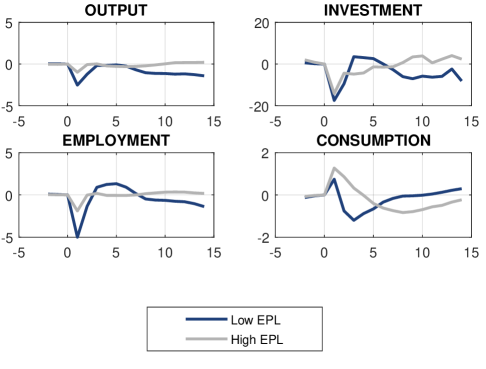
Figure 7: Uncertainty Shocks under high and low labor protection

Notes: This figure presents DSGE impulse responses of output, investment, employment and consumption after an uncertainty shock. Thereby, the blue lines presents the impulse response to uncertainty shock under low employment protection legislation and the gray line shows the impulse response of the same uncertainty shock under high employment protection.

6.2 Evidence from a VAR

Now, we use the international set of revision based measures of uncertainty to test this theoretical prediction. We thus split countries into two groups according to their strictness of employment protection. To split countries according to their degree of employment protection, we use the annual time series data of the OECD Employment Protection Database to calculate the average value of the strictness of employment protection. Specifically, we use the measure of individual and collective dismissals (EPRC_V1) from 1985 to 2013. Table 3 ranks countries according to the strictness of employment protection.

Country	Average EPL (1985-2013)
United States	0.26
Canada	0.92
United Kingdom	1.17
Switzerland	1.60
Median	1.62
Japan	1.62
France	2.39
Germany	2.65
Sweden	2.70
Italy	2.76

Table 3: High EPL vs. low EPL countries

Notes: This table ranks countries according to the strictness of employment protection. In order to calculate the ranking, we use the annual time series data of the OECD Employment Protection Database to calculate the average value of the strictness of employment protection – individual and collective dismissals (EPRC_V1) - over time (from 1985 to 2013).

The groups selected in Table 3 mirror our expectations with Anglo-Saxon economies displaying a low degree and continental European countries showing higher degree of employment protection standards. According to OECD Employment Protection Database, Switzerland and Japan have a very similar degree of EPL. In our baseline specification, we include Switzerland in the group with low labor protection and Japan in the group of high EPL countries. To obtain group-specific impulse responses to an uncertainty shock, we use the VAR described in section 5.2, averaging across country-specific impulse responses for each group. Our empirical findings suggest that uncertainty has indeed less deteriorating effects in countries with high employment protection. Figure 8 shows that the effect of a one standard deviation uncertainty shock is not only more contractionary in countries with high protection compared to countries with low labor protection, the negative effects are also more persistent.

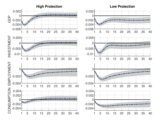
Figure 8: Impulse responses to an uncertainty shock for high EPL countries (left panel) and low EPL countries (right panel).

Notes: The dotted blue line depicts the posterior mean and the grey shaded area the 68% error bands for the impulse responses to an one standard deviation uncertainty shock. The estimation sample spans the period 1988Q1–2019Q4.

The results presented in Figure 8 are consistent with the theoretical predictions outlined above. In countries with stricter employment protection legislation, it is more costly for firms to reduce employment. Hence, employment drops less in the light of an uncertainty shock. Because of the lower response of employment and because of the complementarity of capital and labor, firms do not cut investment by as much, causing production to contract less. Finally, uncertainty decreases consumption less in countries with high labor protection. As pointed out in 6.1, an uncertainty shock increases the misallocation in an economy more if firing costs are higher. Households expect the increased missalocation to decrease future return on savings and they decrease consumption less. While this mechanism might explain parts of the differences in the consumption dynamics, precautionary saving might also be part of the story. A higher degree of labor protection transmits into a higher job security of employees. An increase in uncertainty lets employees worry less about their future income in case of high employment protection than in case of low employment protection. Households thus increase precautionary saving less and decrease consumption by less which causes a less pronounced drop of aggregate demand. Our findings are consistent with the evidence presented by Jo and Lee (2019) that indicates that compared to Germany, labor market frictions in the U.S. might be too low for uncertainty to have strong real option effects on employment. Our evidence complements the literature on the importance of the labor channel in explaining the transmission of uncertainty shocks. However, it highlights a different mechanism. In contrast to Guglielminetti (2016), who argues for the importance of hiring costs, our results indicate a prominent role of firing costs in explaining the dynamics of uncertainty shocks.

7 Conclusion

In this paper we have introduced new internationally comparable measures of macroeconomic uncertainty for a large set of countries using data revisions in aggregate variable that are bound to the system of national accounts. We have set up an econometric model and constructed a new real-time data set of real GDP for 39 countries that serves as the basis for our estimations. Using real-time data permits us to obtain accurate estimates of forecast error based uncertainty that an economic agent experienced at any given point in time, whereas existing measures of macroeconomic uncertainty base on forecast errors that are constructed with non real-time data.

In order to obtain real-time uncertainty estimates, we extended the data revision model proposed by Jacobs and van Norden (2011) such that it allows us to extract the volatility of the unpredictable part of future releases of the news component that forms our measure of macroeconomic uncertainty. We showed that the resulting uncertainty indicator for the United States has similar properties than the macroeconomic uncertainty measures proposed by Jurado et al. (2015). The revision based indicator is thereby less volatile than alternative measures such as the economic policy uncertainty index by Baker et al. (2016) or the VIX and the revision based indicator also identifies the same three major uncertainty shocks between 1965 and 2016. Namely, the recession in the 1970s, the early 1980s recession and the Great Recession of 2008. The revision based indicator reaches its highest peak during 1970s. Considering that the recession in the 1970s comprised the first oil price shocks, the collapse of the Bretton Woods System and the end of the post World War II economic expansion this seems coherent with a broader economic history perspective. Our empirical evaluation indicates a strong and negative relationship between the revision based uncertainty measures and the economy. Estimating VARs for the United States and the G7 countries shows that a one standard deviation shock in the revision based uncertainty indicators leads to a contraction in GDP, investment, employment and consumption.

We studied the importance of labor market frictions for the propagation of uncertainty shocks. In a cross-country VAR analysis, we found that uncertainty shocks have more deteriorating effects in countries with a lower degree of EPL compared to countries with stricter EPL. Using the theoretical model of Bloom et al. (2018) with varying degree of firing costs, we show that these empirical findings are in line with theory.

Appendix A Posterior Simulations

In this section we describe the blocks of our Gibbs sampling procedure outlined in section 2. Note that Equations (2) and (6) can be rewritten as

$$Y_{t} =Z\alpha_{t},$$ (12)

$$\alpha_{t} =\varphi_{t}+T_{t}\alpha_{t-1}+RD_{t}^{1/2}\eta_{t},$$ (13)

with

$$R=\begin{bmatrix}1&1&0&0\\ 0&-1&0&0\\ 0&0&0&0\\ 0&0&1&0\\ 0&0&0&1\end{bmatrix},D_{t}=\begin{bmatrix}\exp(h_{t}^{\nu 1})&0&0&0\\ 0&\exp(h_{t}^{\nu L})&0&0\\ 0&0&\exp(h_{t}^{\zeta 1})&0\\ 0&0&0&\exp(h_{t}^{\zeta L})\end{bmatrix}.$$

A.1 Drawing News, Noise and True Values

Conditional on the stochastic volatilities and the VAR coefficients of the state space model ($c_{t}$ and $\rho_{t}$), we draw $\alpha_{t}$ for $t=1,..,T$, using the forward filtering backward sampling procedure of Carter and Kohn (1994) and Frühwirth-Schnatter (1994), where (12) serves as observation equation and (13) as state equation.

A.2 Drawing Stochastic Volatility

Conditional on news, noise, true values and the VAR coefficients of (13), we obtain draws for the stochastic volatilities ($h_{t}^{x}$) using the estimation method proposed in Kastner and Frühwirth-Schnatter (2014). We thus estimate the stochastic volatilities by interweaving estimation models specified in a centered (C) and a non-centered (NC) parameterization using the ancillarity-sufficiency interweaving strategy (ASIS) detailed by Yu and Meng (2011). This estimation strategy addresses the trade-off in terms of sampling efficiency depending on the value of the persistence parameter $\phi$. Kastner and Frühwirth-Schnatter (2014) show that this estimation strategy outperforms estimators using pure centered or non-centered parameterizations.

Starting from Equation (4), we assume that:

$$\sigma^{i}_{t}\eta^{i}_{t} =e^{h_{t}^{i}/2}\eta^{i}_{t}$$ (14)

$$h_{t}^{i} =\mu^{i}+\phi^{i}(h_{t-1}^{i}-\mu^{i})+\tau^{i}\epsilon_{t}^{i}\text{\ \ },$$ (15)

with $\epsilon_{t}^{i}\sim N(0,1)$ and $x=\nu 1,\nu L,\zeta 1,\zeta L$. One can express the centered parametrization of Equation (17) as a non-centered parametrization. In the non-centered parametrization the volatility components are assumed to follow the following process:

$$\tilde{h}_{t}^{i}=\phi^{i}\tilde{h}_{t-1}^{i}+\epsilon_{t}^{i},$$ (16)

with $\epsilon_{t}^{i}\sim N(0,1)$ and $x=\nu 1,\nu L,\zeta 1,\zeta L$.

We can rewrite Equation (14) as

$$\tilde{\sigma}^{i}_{t}=h^{i}_{t}+log((\eta^{i}_{t})^{2})$$ (17)

with $\eta^{i}_{t}\sim N(0,1)$ and $\tilde{\sigma}^{i}_{t}$ denotes $log((\sigma^{i}_{t}\eta^{i}_{t})^{2})$. The fact that we can approximate the distribution of $log((\eta^{i}_{t})^{2})$ by a mixture of normal distributions, that is, $log((\eta^{i}_{t})^{2})|r^{i}_{t}\sim N(m^{i}_{r_{t}},(s^{i})^{2}_{r_{t}})$ with $r_{t}$ indicating the mixture component, we can rewrite Equation (17) as a linear and conditionally Gaussian state space model,

$$\tilde{\sigma}^{i}_{t}=m_{r_{t}}^{i}+h^{i}_{t}+\eta^{i}_{t},$$ (18)

with $\eta^{i}_{t}\sim N(0,s^{{2}^{i}_{r_{t}}})$. Based on Equation (18), we apply a MCMC procedure outlined in Kastner and Frühwirth-Schnatter (2014) that interweaves the centered and non-centered specification.

We rely on the priors proposed in Kastner and Frühwirth-Schnatter (2014). That is, $\mu$ follows a normal distribution with mean $b_{\mu}$ and variance $B_{\mu}$, i.e. $\mu\sim N(b_{\mu},B_{\mu})$. The persistence parameter $\phi$ follows a Beta distribution, i.e. $B(a_{0},b_{0})$. Finally, for the volatility parameter $\sigma$, they chose $\sigma^{2}\sim B_{\sigma}\chi^{2}_{1}=G(1/2,1/2B_{\sigma})$. We use the same priors for the centered and non-centered parameterization. We calibrate the parameters as follows: $b_{\mu}=0$, $B_{\mu}=100$, $a_{0}=5$, $b_{0}=1.5$ and $B_{\sigma}=1$.

The MCMC interweaving procedure consists of the following steps:

1. We sample the volatilities using the all without a loop (AWOL) procedure by drawing from $h_{[-0]}^{i}|\tilde{\sigma}^{i},r^{i},\mu^{i},\phi^{i},(\eta^{i})^{2}$. The initial values are drawn from $h_{0}^{i}|h_{1}^{i},r^{i},\mu^{i},\phi^{i},(\eta^{i})^{2}$.

2. We sample $\mu^{i},\phi^{i}$, and $(\eta^{i})^{2}$ using Bayesian regression. We use a 2-block sampler, where we draw $(\eta^{i})^{2}$ from $(\eta^{i})^{2}|h^{i},\mu^{i},\phi^{i}$ and we jointly sample $\mu^{i}$ and $\phi^{i}$ from $\mu^{i},\phi^{i}|h^{i},(\eta^{i})^{2}$. Because the chosen priors are not analytically tractable, we calculate updates via a Metropolis-Hastings (MH) algorithm.

3. Move to NC by the deterministic transformation $\tilde{h_{t}^{i}}=\frac{h_{t}^{i}-\mu^{i}}{\eta^{i}}$

4. Redraw $\mu^{i},\phi^{i},(\eta^{i})^{2}$ for NC specification. We need MH only to update $\phi^{i}$ by drawing from $\phi^{i}|\tilde{h}^{i}$. We can Gibbs-update $\mu^{i}$ and $(\eta^{i})^{2}$ jointly from $\mu^{i},(\eta^{i})^{2}|\tilde{\sigma}^{i},\tilde{h}^{i},r^{i}$.

5. Move back to C by calculating $h_{t}^{i}=\mu^{i}+\eta^{i}\tilde{h}_{t}^{i}$ for all t

6. Draw the indicators $r^{i}$ (C). We update the mixture component indicators $r^{i}$ from $r^{i}|\tilde{\sigma}^{i}$ using inverse transform sampling.

A.3 Drawing Time-Varying Coefficients

Conditional on news, noise, true values and the stochastic volatilities, we draw the time-varying coefficients of Equation (13), by considering the process of true GDP $\tilde{y}_{t}$ to be represented by the following state space model

$$\tilde{y}_{t} =Z_{t}\alpha_{t}+G_{t}u_{t},$$ (19)

$$\alpha_{t} =T\alpha_{t-1}+H_{i,j}e_{t}$$ (20)

with

$$Z_{t}=\begin{bmatrix}1&\tilde{y}_{t}\end{bmatrix},\alpha_{t}=\begin{bmatrix}c_{t}\\ \rho_{t}\end{bmatrix}G_{t}=\begin{bmatrix}\exp(h_{t}^{\nu 1})&\exp(h_{t}^{\nu L})\end{bmatrix},$$ (21)

$$u_{t}=\begin{bmatrix}u_{t}^{\nu 1}\\ u_{t}^{\nu L}\end{bmatrix},T=\begin{bmatrix}1&0\\ 0&1\end{bmatrix},H_{i,j}=\begin{bmatrix}\sigma_{i,j}^{c_{i,j}}&\sigma_{i,j}^{\rho_{i,j}}\end{bmatrix},e_{t}=\begin{bmatrix}e_{t}^{c_{t}}\\ e_{t}^{\rho_{t}}\end{bmatrix}.$$

We obtain estimates for $c_{t}$ and $\rho_{t}$ using the method proposed by McCausland et al. (2011). We set up the diagonal matrix $\Omega$ as follows:

Diagonal Matrix $\Omega$

$$\Omega=\begin{bmatrix}\Omega_{11}&\Omega_{t/t-1}&0&\cdots&0\\ \Omega_{t/t-1}&\Omega_{tt}&\Omega_{t/t-1}&\ddots&\vdots\\ 0&\Omega_{t/t-1}&\ddots&\ddots&0\\ \vdots&\ddots&\ddots&\Omega_{tt}&\Omega_{t/t-1}\\ 0&\cdots&0&\Omega_{t/t-1}&\Omega_{nn}\\ \end{bmatrix}$$ (22)

Diagonal Elements

$$\Omega_{11} =Z_{1}^{\prime}A_{11,1}Z_{1}+A_{22,1}+P_{1}^{-1}$$ (23)

$$\Omega_{tt} =Z_{t}^{\prime}A_{11,t}Z_{t}+2A_{22,t}$$ (24)

$$\Omega_{nn} =Z_{n}^{\prime}A_{11,n}Z_{n}+A_{22,n}$$ (25)

Off-Diagonal Elements

$$\Omega_{t/t-1} =-A_{22,t}$$ (27)

with

$$A_{t} =\begin{bmatrix}(G_{t}\ ^{\prime}\ G_{t})^{-1}&0\\ 0&(H_{i,j}\ ^{\prime}\ H_{i,j})^{-1}\end{bmatrix}$$ (29)

We set up the co-vector $C$ the following way:

Covector

$$C_{1}=\begin{bmatrix}C_{1}\\ C_{tt}\\ \vdots\\ C_{nn}\\ \end{bmatrix}.$$ (31)

with

$$C_{1} =Z_{0}^{\prime}A_{11,0}\tilde{y}_{0}+P_{1}^{-1}a_{1}$$ (32)

$$C_{tt} =Z_{t}^{\prime}A_{11,t}\tilde{y}_{t}$$ (33)

$$C_{nn} =Z_{T}^{\prime}A_{11,T}\tilde{y}_{T}$$ (34)

We solve this system by first computing the Cholesky decomposition $\Omega=LL^{\prime}$ that we implement directly in Julia. Because of the band structure of $\Omega$, the decomposition is incredibly fast. In a second step, we draw $e_{t}\sim N(0,1)$ and solve $La=c$ for $a$. Finally, we use back-substitution in order to solve $L^{\prime}h=a+e$ for $h$.

Appendix B Real-Time Data

We use data revisions in macroeconomic aggregates to obtain measures of macroeconomic uncertainty for various OECD countries. Real-time data releases of macroeconomic aggregates are thereby the key ingredient to construct the uncertainty indicator. In our preferred specification, we base the indicator on nominal GDP. In order to obtain a comprehensive data set for various countries, we need to tap and combine several data sources. Appendix B describes these various data sources and outlines the construction of our data base in great detail.

B.1 Real-Time Data: Main Source

The largest part of our data is provided by Original Release Data and Revisions Database. The Original Release Data and Revisions Database is part of OECD Main Economic Indicators database (OECD, 2017) and represents the central data source of this project. The database provides different releases of macroeconomic aggregates for many countries. This study uses data from 32 countries including Australia, Austria, Belgium, Brazil, Canada, Denmark, Finland, France, Germany, Great Britain, Greece, Iceland, India, Indonesia, Ireland, Israel, Italy, Japan, Korea, Luxembourg, Mexico, Netherlands, New Zealand, Norway, Portugal, Russia, South Africa, Spain, Sweden, Switzerland, Turkey, USA. Unfortunately, Original Release Data and Revisions Database provides releases of macroeconomic variables only since 1999. For data prior to 1999, we need to rely on other data providers. We primarily use the data made available by the Federal Reserve of Dallas for releases prior to 1999. Fernandez et al. (2011) collect real-time data for various economies including those that we use in this study. The authors assemble the dataset from original quarterly releases of different macroeconomic aggregates from 1962 to 1998. We use their data for all countries except the Australia, New Zealand, and U.S.. For the U.S., we use data provided by the Federal Reserve of Philadelphia as they provide more exhaustive data compared to the data provided by Federal Reserve of Dallas. We use Australian nominal GDP data provided by the Australian Real-Time Macroeconomic Database (Lee et al. (2012)). For New Zealand, we use the “Real-Time GDP Data” data set from the Reserve Bank of New Zealand that provides nominal GDP releases. Table 1 provides an overview of the countries included in our study, the data provider and the first available data point.

Figure 9 shows the average of the 10th revision of year-over-year growth rates of nominal GDP. Thereby, most countries have a statistical significant downward bias. That is, ten quarter after the first release, most countries countries publish on average a higher growth rate.

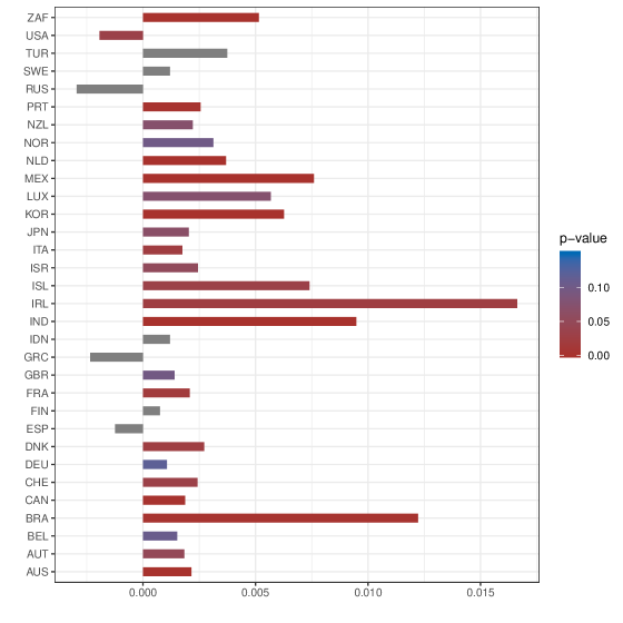
Figure 9: Real GDP Growth (yoy): Mean of the 10th revisions for the period from 2000 Q1 to 2016Q3.

B.2 Real-Time Data: Practical decisions

Australia
We use real-time data from the Real-Time Macroeconomic Database provided by the University Melbourne Macroeconomics Research Unit. The 1973Q3 vintage contains unusual entries. The 1973Q2 vintage contains combined figures for the 1972Q3-Q4 and 1973Q1-Q2 reference dates. We split the combined figures by using the share of the 1973Q4 vintage.

Canada
We use real-time data provided by the Federal Reserve of Dallas for releases prior to 1982. For the time span between 1982 and 1999, we rely on real-time data provided by the Bank of Canada. Finally, from 1999 onward, we use real-time data provided by the OECD Main Economic Indicators database. The data provided by the OECD Main Economic Indicators database and the Bank of England are virtually identical after 1999, expect for the quarters 2000Q2 to 2001Q1. For this quarter, we opt for data provided by the Bank of Canada as they appear to be by far less volatile.

Germany
We use real-time data provided by the Federal Reserve of Dallas for releases prior to 1999. The dataset provides GNP until February 1993. Thereafter the dataset provided by the Federal Reserve of Dallas contains data on GDP. Furthermore, the dataset contains vintages for West Germany until November 1993. From February 1994 on-wards, the dataset provides vintages for the unified Germany. Unfortunately, the length of the vintages between February 1994 and August 1995 is critically short. Hence, we use vintages of GNP for West Germany until May 1995 (provided by Boysen-Hogrefe and Neuwirth (2012)). From August 1995 onwards, we use GDP for united Germany provided by the Federal Reserve of Dallas. Finally, starting from 1999, we use data on GDP provided by the OECD Main Economic Indicators database.

B.3 VAR Data

Quarterly GDP Japan
We obtain quarterly real GDP for Japan from 1994Q1 until now from the OECD database. The Economic and Social Research Institute of Japan provides Real GDP Growth prior to 1994 at 2000 prices that is used to calculated from Real GDP until 1980. Real GDP Growth prior to Q1 1981 is calculated from the last growth rate of of each window for a certain quarter from our release dataset.

B.4 Benchmark Revisions

In this paper, we separate revisions of macroeconomic variables into revisions because of news and revisions because of noise. However, besides news and noise, there exists an additional source of revisions that we have not considered so far: benchmark or comprehensive revisions. While revisions because of news and noise represents revisions in the data that are because of new information or measurement errors, benchmark revisions represent revisions in the data that are because of changes in the GDP calculation process. These revisions can include the incorporation of new data sources as well as the adaptation of major changes in the statistical methodology. In addition, Benchmark revisions can be because of changes in the GDP definition. As the economy evolves over time, i.e. new sector appear, others disappear, the definition of GDP needs to be adopted to fit best the evolved structure of the economy. Benchmark revisions usually take place every four to five years and comprise comprehensive changes to the way GDP is calculates. Since World War II the were 15 benchmark revisions in the United States (see Table 4).

Table 4: NIPA Comprehensive Revisions

Number	Date		Number	Date
1st	July 1947		9th	December 1991
2nd	July 1951		10th	January 1996
3rd	July 1954		11th	October 1999
4th	July 1958		12th	December 2003
5th	August 1965		13th	July 2009
6th	January 1976		14th	July 2013
7th	December 1980		15th	July 2018
8th	December 1985

Notes: The table lists the dates of the 15^th comprehensive revisions of the U.S. National Income and Product Accounts (NIPA) since World War II. The dating of the comprehensive revisions is taken from Fox et al. (2017) for the 1^st to the 14^th revision. The date of the 15^th comprehensive revisions is taken from the BEA website (https://apps.bea.gov/scb/2018/04-april/0418-preview-2018-comprehensive-nipa-update.htm). Green rows mark comprehensive revisions that are within the years covered by our uncertainty measure for the United States. Rows in red mark comprehensive revisions prior to the start of our uncertainty measure.

Benchmark revisions can lead to large and significant revisions in the level of macroeconomic variables. Large revisions in GDP that are not because news or noise would of course be a concern for our estimation procedure. Luckily, while benchmark revisions can lead to significant changes in levels, growth rates of macroeconomic variables are much less effected by benchmark revisions. However, even though benchmark revisions are much less of a concern when working with growth rates, we still want to examine if benchmark revision have a systematic effect on our uncertainty measure. Figure 10 plots our uncertainty indicator and highlights the various benchmark revisions. Overall, we have 10 benchmark revisions that occurred during the time period covered by our indicator. Figure 10 does not expose any clear pattern of influence. While some benchmark revision occurred close to spikes of our indicator, others occur in periods where our indicator does not react at all. We take this as descriptive evidence that benchmark revisions are unlikely to systematically cause major spikes of our uncertainty indicator.

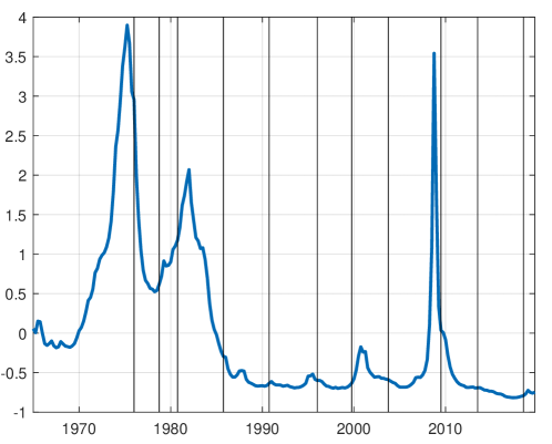
Figure 10: Impact of Benchmark Revisions

Notes: The figure presents the macroeconomic uncertainty indicator for the United States and highlights the dates of relevant benchmark revisions. The dates of the benchmark revisions correspond to the dates of Table 4.

Appendix C Uncertainty Estimates

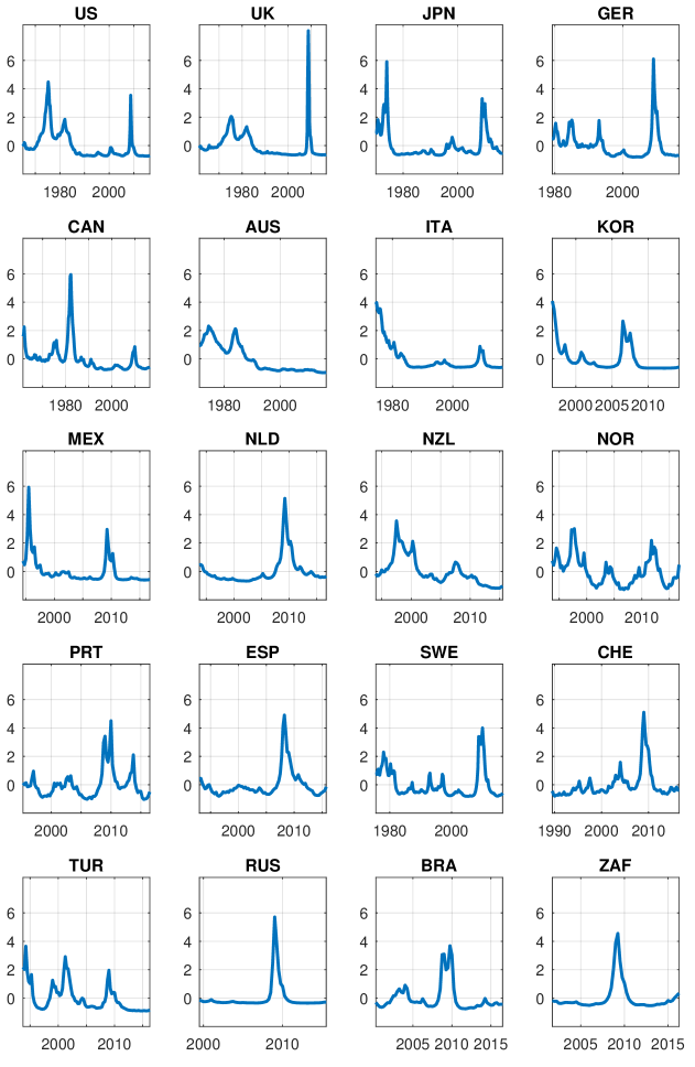
Figure 11: Macroeconomic Uncertainty

Notes: This figure presents uncertainty indicators based on real GDP growth revisions. All indicators are demeaned and standardized to unit variance.

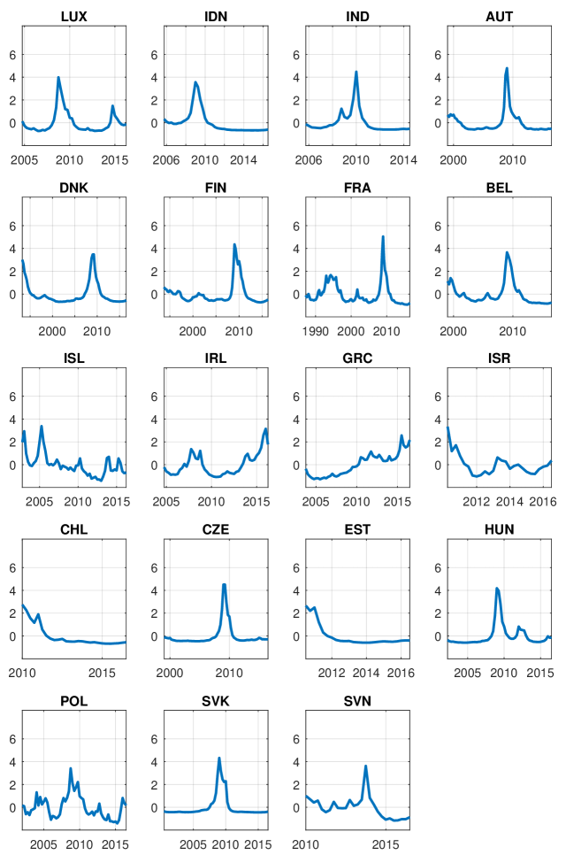
Figure 12: Macroeconomic Uncertainty (cont.)

Notes: This figure presents uncertainty indicators based on real GDP growth revisions. All indicator are demeaned and standardized to unit variance.

Appendix D Information Content of the First Release of GDP

Statistical agencies publish the first GDP figure for a given quarter about one month after the end of a quarter. At that point in time, they do not have all information necessary to compute the GDP. Thus, some parts of GDP need to be estimated. While little is known about the exact estimation procedure applied by statistical agencies, Scruton et al. (2018) describe the GDP data collection process of the Office for National Statistics (ONS) in the United Kingdom. In their report, the authors describe the ONS GDP publication routine that was valid until 2018. The ONS publishes three GDP releases per quarter. The first figure of GDP is released about 25 days after the end of a quarter. At this point in time, ONS has only output data at their disposal. The available information content corresponds to about 45%. The rest needs to be forecasted by ONS. Scruton et al. (2018) state that ONS forecasts large parts of the final month of a quarter as less data tend to be available for the last month of a quarter compared to the previous two months. Approximately two months after the end of a quarter, ONS publishes the second estimate of GDP. This estimate builds already on a significantly larger information set and includes, besides output data also data on income and expenditure.The overall data content amounts to approximately 65%. ONS publishes the third estimate of GDP roughly 85 days after the end of a quarter and the overall data content contained in the estimate amounts to approximately 90%.

The insights provided by Scruton et al. (2018) supports our view that one can interpret the first release of GDP as a forecast by statistical agencies for the final true GDP. In this paper, we treat the first published year-over-year growth rate of real GDP as a forecast for the final release of GDP, which we define as the year-over-year growth rate released after 3 years. This view allows us to compute quarterly forecast error made by the statistical agencies. We follow the idea by Jurado et al. (2015) and compute the conditional volatility of the forecast error series which we define as our measure of macroeconomic uncertainty. Thus, this paper presumes that GDP forms a good summary of the macroeconomic activity in an economy.

In their paper, Jurado et al. (2015) argue that it is important to remove the entire forecastable component of a forecast error in order to obtain the true unpredictable part of a forecast. Otherwise the explainable part will incorrectly end up in the uncertainty component. In order to obtain the unpredictable part of the GDP revisions (i.e., the unpredictable forecast errors committed by a statistical agent), we use the model outlined in Section 2. Our measure of macroeconomic uncertainty is defined as the conditional volatility of the error corresponding to the unpredictable part of revisions in GDP growth rates.

Despite the decomposition of the revisions in into news and noise, it is key to understand the information content of the first release of GDP for the last release. In other words, we need to understand if the first release of GDP is a good forecast for the final GDP. Ideally, we want the first release to be the best available forecast for the final release of GDP. Given this central importance for our uncertainty measure, we test the information content of the first release of U.S. GDP for the last release of U.S. GDP by conducting a forecasting horse race.

In this forecasting horse race, we treat the first release itself as a forecast and the difference between the last release and the first release as forecast errors. Doing so allows us to compute the RMSE of these forecast errors and compare it to the following two pseudo out-of-sample forecast exercises for the final U.S. GDP release. Both forecasting exercises use the econometric framework outlined in Section 2 in Jurado et al. (2015) to forecast last release of GDP.

The first forecasting exercises uses the 132 macroeconomic variables and the 147 financial variables proposed by Jurado et al. (2015) to forecast the final GDP release. In order to conduct this forecast, we use the original dataset provided by the authors in their Online-Appendix. As the dataset contains monthly time series, but we need to forecast quarterly GDP, we aggregate the monthly series to quarterly series by taking quarterly averages. Real-time GDP for the U.S. starts in 1965Q1. The dataset by Jurado et al. (2015) provides data up to 2011Q4. We conduct pseudo out-of-sample forecasts for the quarter 1976Q4 to 2011Q4. In the second exercise, we repeat the first exercise, but use the least release as an additional predictor.

This analysis shows that for the United States the first release of GDP appears to be a good forecast for the final GDP. We can show that when using established forecast routines and one of the most comprehensive dataset about the U.S. economy, we cannot beat the forecast performance of the first release.

Table 5: Comparison Forecast Performance

	First Release	JLN	JLN
	(as forecast for last release)		+First Release
RSME	0.00752	0.00807	0.00816
Ratio (RMSE Only First Release)	1.000	1.072	1.084

Notes: The table compares the forecast accuracy in predicting the final year-over-year growth of real GDP in the United States. The first column refers to the forecast performance of the first release for the last release. The second column reports the performance of the forecasting model proposed by Jurado et al. (2015). The last column refers to the model of Jurado et al. (2015) augmented with the first release as an additional predictor. In the first row, we display the RMSE error of the different specifications. The second row reports the RMSEs relative to the RMSE of the first release.

Appendix E Robustness

E.1 Selected High and Low EPL Countries

In order to empirically evaluate the effect of employment protection legislation (EPL) on the propagation of uncertainty shocks, we estimate a VAR for countries with stricter EPL and a VAR for countries with a lower degree of EPL. As mentioned in the main text, we use the OECD Employment Protection Database to split countries into two groups. The groups selected in Table 3 mirror our expectations with Anglo-Saxon economies displaying a low degree and continental European countries showing higher degree of employment protection standards. The OECD Employment Protection Database attests Switzerland and Japan have a very similar degree of employment protection legislation. In our baseline specification, we include Switzerland in the group with low labor protection and Japan in the group of high EPL countries. As a robustness test, we re-run the analysis excluding both Japan and Switzerland. Figure 13 shows that neglecting the two countries does not significantly change the results. Estimating a pooled VAR for both groups shows that uncertainty has still less deteriorating effects in countries with high employment protection.

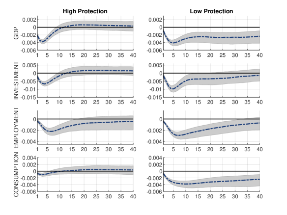
Figure 13: Impulse responses to an uncertainty shock for high EPL countries (left panel) and low EPL countries (right panel) without Japan and Switzerland.

Notes: The dotted blue line depicts the posterior mean and the grey shaded area the 68% error bands for the impulse responses to an one standard deviation uncertainty shock. The estimation sample spans the period 1988Q1–2016Q3.

E.2 Incorporating Estimation Uncertainty

We now investigate the impact of the estimation uncertainty surrounding our measures of macroeconomic uncertainty on our main findings. Instead of using the mean of the posterior distribution of our uncertainty measure, we now simulate the posterior distribution of the VAR model conditional on the draws from the posterior distribution of our uncertainty indicator. Figure 14 compares the impulse responses functions of high protection countries to low protection countries. Although the overall effects are somewhat weaker than the ones shown in Figure 8, the relative precision does not change in a significant manner. Most importantly, our principal findings do not change when taking into account the uncertainty surrounding our uncertainty estimates. Figure 15 presents the overall effects for the G7 average. The responses of the variables seem also somewhat weaker than the ones reported in Figure 6. The impulse response functions of consumption are additionally not clearly negative anymore. The impulse responses for all other variable however appear robust with regards to the inclusion of the added estimation uncertainty.

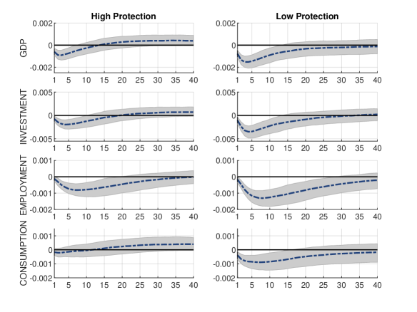
Figure 14: Impulse responses to an uncertainty shock for high EPL countries (left panel) and low EPL countries (right panel), including the uncertainty surrounding data revisions based uncertainty indicator.

Notes: The dotted blue line depicts the posterior mean and the grey shaded area the 68% error bands for the impulse responses to an one standard deviation uncertainty shock. The estimation sample spans the period 1988Q1–2016Q3.

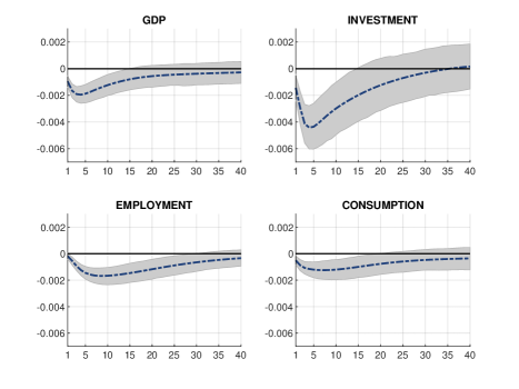
Figure 15: Impulse responses to an uncertainty shock for the group of G7 countries, including the uncertainty surrounding data revisions based uncertainty indicator.

Notes: The dotted blue line depicts the posterior mean and the grey shaded area the 68% error bands for the impulse responses to an one standard deviation uncertainty shock. The estimation sample spans the period 1988Q1–2016Q3.

References

- Ahir et al. (2018) H. Ahir, N. Bloom, and D. Furceri. The world uncertainty index. Available at SSRN 3275033, 2018.
- Altig et al. (2020) D. Altig, S. Baker, J. M. Barrero, N. Bloom, P. Bunn, S. Chen, S. J. Davis, J. Leather, B. Meyer, E. Mihaylov, et al. Economic uncertainty before and during the covid-19 pandemic. Journal of Public Economics, 191:104274, 2020.
- Baker et al. (2016) S. R. Baker, N. Bloom, and S. J. Davis. Measuring economic policy uncertainty. The Quarterly Journal of Economics, 131(4):1593–1636, 2016.
- Basu and Bundick (2017) S. Basu and B. Bundick. Uncertainty shocks in a model of effective demand. Econometrica, 85(3):937–958, 2017.
- Bell (2016) U.-L. Bell. Adjustment costs, uncertainty and employment inertia. Working Paper Series Bank of Spain, (9620), 2016.
- Berger et al. (2017) T. Berger, S. Grabert, and B. Kempa. Global macroeconomic uncertainty. Journal of Macroeconomics, 53:42–56, 2017.
- Bloom (2009) N. Bloom. The impact of uncertainty shocks. Econometrica, 77(3):623–685, 2009. ISSN 1468-0262. doi: 10.3982/ECTA6248. URL http://dx.doi.org/10.3982/ECTA6248.
- Bloom (2014) N. Bloom. Fluctuations in uncertainty. Journal of Economic Perspectives, 28(2):153–76, 2014. doi: 10.1257/jep.28.2.153. URL http://www.aeaweb.org/articles.php?doi=10.1257/jep.28.2.153.
- Bloom et al. (2018) N. Bloom, M. Floetotto, N. Jaimovich, I. Saporta-Eksten, and S. J. Terry. Really uncertain business cycles. Econometrica, 86(3):1031–1065, 2018.
- Boysen-Hogrefe and Neuwirth (2012) J. Boysen-Hogrefe and S. Neuwirth. The impact of seasonal and price adjustments on the predictability of german gdp revisions. Technical report, Kiel Working Paper, 2012.
- Cacciatore and Ravenna (2015) M. Cacciatore and F. Ravenna. Uncertainty, wages, and the business cycle. In 29th Annual Meeting of the Canadian Macroeconomics Study Group, Montréal, pages 6–7, 2015.
- Caggiano et al. (2014) G. Caggiano, E. Castelnuovo, and N. Groshenny. Uncertainty shocks and unemployment dynamics in us recessions. Journal of Monetary Economics, 67:78–92, 2014.
- Caggiano et al. (2017) G. Caggiano, E. Castelnuovo, and J. M. Figueres. Economic policy uncertainty and unemployment in the united states: A nonlinear approach. Economics Letters, 151:31–34, 2017.
- Caggiano et al. (2020) G. Caggiano, E. Castelnuovo, and J. M. Figueres. Global uncertainty. mimeo, 2020.
- Caldara et al. (2016) D. Caldara, C. Fuentes-Albero, S. Gilchrist, and E. Zakrajšek. The macroeconomic impact of financial and uncertainty shocks. European Economic Review, 88:185–207, 2016.
- Carriero et al. (2018) A. Carriero, T. E. Clark, and M. Marcellino. Measuring uncertainty and its impact on the economy. Review of Economics and Statistics, 100(5):799–815, 2018.
- Carriero et al. (2019) A. Carriero, T. E. Clark, and M. Marcellino. Asssessing international commonality in macroeconomic uncertainty and its effects. Journal of Applied Econometrics, 2019.
- Carter and Kohn (1994) C. K. Carter and R. Kohn. On Gibbs sampling for state space models. Biometrika, 81(3):541–553, 09 1994.
- Cascaldi-Garcia et al. (2020) D. Cascaldi-Garcia, D. Datta, T. RT Ferreira, O. V. Grishchenko, M. R. Jahan-Parvar, J. M. Londono, F. Loria, S. Ma, M. Rodriguez, J. H. Rogers, et al. What is certain about uncertainty? Olesya V. and Jahan-Parvar, Mohammad R. and Londono-Yarce, Juan-Miguel and Loria, Francesca and Ma, Sai and Rodriguez, Marius and Rogers, John H. and Sarisoy, Cisil and Zer, Ilknur, What is Certain About Uncertainty, 2020.
- Castelnuovo (2019) E. Castelnuovo. Domestic and global uncertainty: A survey and some new results. CESifo Working Paper Series, (7900), 2019.
- Choi and Loungani (2015) S. Choi and P. Loungani. Uncertainty and unemployment: The effects of aggregate and sectoral channels. Journal of Macroeconomics, 46:344–358, 2015.
- Clark et al. (2020) T. E. Clark, M. W. McCracken, and E. Mertens. Modeling time-varying uncertainty of multiple-horizon forecast errors. The Review of Economics and Statistics, 102(1):17–33, 2020.
- Cogley and Sargent (2005) T. Cogley and T. J. Sargent. Drifts and volatilities: monetary policies and outcomes in the post wwii us. Review of Economic Dynamics, 8(2):262 – 302, 2005. ISSN 1094-2025. doi: https://doi.org/10.1016/j.red.2004.10.009. URL http://www.sciencedirect.com/science/article/pii/S1094202505000049. Monetary Policy and Learning.
- Croushore and Stark (2001) D. Croushore and T. Stark. A real-time data set for macroeconomists. Journal of Econometrics, 105(1):111 – 130, 2001. ISSN 0304-4076. doi: https://doi.org/10.1016/S0304-4076(01)00072-0. URL http://www.sciencedirect.com/science/article/pii/S0304407601000720. Forecasting and empirical methods in finance and macroeconomics.
- Davis (2016) S. J. Davis. An index of global economic policy uncertainty. Technical report, National Bureau of Economic Research, 2016.
- de Jong (1987) P. de Jong. Rational economic data revisions. Journal of Business & Economic Statistics, 5(4):539–548, 1987.
- Del Boca and Rota (1998) A. Del Boca and P. Rota. How much does hiring and firing cost? survey evidence from a sample of italian firms. Labour, 12(3):427–449, 1998.
- Fernandez et al. (2011) A. Z. Fernandez, H. Branch, E. F. Koenig, and A. Nikolsko-Rzhevskyy. A real-time historical database for the oecd. Globalization and Monetary Policy Institute Working Paper, 96, 2011.
- Fernández-Villaverde and Guerrón-Quintana (2020) J. Fernández-Villaverde and P. A. Guerrón-Quintana. Uncertainty shocks and business cycle research. Technical report, National Bureau of Economic Research, 2020.
- Fox et al. (2017) D. R. Fox, S. H. McCulla, S. Smith, E. P. Seskin, E. Strassner, D. B. Wasshausen, B. R. Moulton, C. E. Moylan, and N. M. Mayerhauser. Methods of the us national income and product account. US Department of Commerce, Bureau of Economic Analysis: Washington, WA, USA, page 447, November 2017.
- Frühwirth-Schnatter (1994) S. Frühwirth-Schnatter. Data augmentation and dynamic linear models. Journal of Time Series Analysis, 15(2), 1994.
- Gilchrist and Zakrajšek (2012) S. Gilchrist and E. Zakrajšek. Credit spreads and business cycle fluctuations. American Economic Review, 102(4):1692–1720, 2012.
- Golinelli and Parigi (2008) R. Golinelli and G. Parigi. Real-time squared: A real-time data set for real-time gdp forecasting. International Journal of Forecasting, 24(3):368–385, 2008.
- Grund (2006) C. Grund. Severance payments for dismissed employees in germany. European Journal of Law and Economics, 22(1):49–71, 2006.
- Guglielminetti (2016) E. Guglielminetti. The labor market channel of macroeconomic uncertainty. Bank of Italy Temi di Discussione (Working Paper) No, 1068, 2016.
- Harmsen et al. (2003) H. Harmsen, L. Meeuwesen, J. Van Wieringen, R. Bernsen, and M. Bruijnzeels. When cultures meet in general practice: intercultural differences between gps and parents of child patients. Patient education and counseling, 51(2):99–106, 2003.
- Hassan et al. (2020) T. A. Hassan, S. Hollander, L. van Lent, and A. Tahoun. The global impact of brexit uncertainty. Technical report, National Bureau of Economic Research, 2020.
- Jacobs and van Norden (2011) J. P. Jacobs and S. van Norden. Modeling data revisions: Measurement error and dynamics of ”true” values. Journal of Econometrics, 161(2):101–109, 2011. URL https://EconPapers.repec.org/RePEc:eee:econom:v:161:y:2011:i:2:p:101-109.
- Jacobs et al. (2020) J. P. Jacobs, S. Sarferaz, J.-E. Sturm, and S. van Norden. Can gdp measurement be further improved? data revision and reconciliation. Journal of Business & Economic Statistics, 2020. URL https://doi.org/10.1080/07350015.2020.1831928.
- Jo and Lee (2019) S. Jo and J. J. Lee. Uncertainty and labor market fluctuations. Technical Report 1904, Federal Reserve Bank of Dallas, 2019.
- Jo and Sekkel (2019) S. Jo and R. Sekkel. Macroeconomic uncertainty through the lens of professional forecasters. Journal of Business & Economic Statistics, 37(3):436–446, 2019. doi: 10.1080/07350015.2017.1356729. URL https://doi.org/10.1080/07350015.2017.1356729.
- Jurado et al. (2015) K. Jurado, S. C. Ludvigson, and S. Ng. Measuring uncertainty. American Economic Review, 105(3):1177–1216, 2015. doi: 10.1257/aer.20131193. URL http://www.aeaweb.org/articles.php?doi=10.1257/aer.20131193.
- Kastner and Frühwirth-Schnatter (2014) G. Kastner and S. Frühwirth-Schnatter. Ancillarity-sufficiency interweaving strategy (asis) for boosting mcmc estimation of stochastic volatility models. Computational Statistics & Data Analysis, 76:408–423, 2014.
- Kim et al. (1998) S. Kim, N. Shephard, and S. Chib. Stochastic volatility: Likelihood inference and comparison with arch models. The Review of Economic Studies, 65(3):361–393, 1998. ISSN 00346527, 1467937X. URL http://www.jstor.org/stable/2566931.
- Kishor and Koenig (2012) K. Kishor and E. F. Koenig. Var estimation and forecasting when data are subject to revision. Journal of Business & Economic Statistics, 30(2):181–190, 2012.
- Kramarz and Michaud (2010) F. Kramarz and M.-L. Michaud. The shape of hiring and separation costs in france. Labour Economics, 17(1):27–37, 2010.
- Kwon et al. (2009) K. Kwon, G. A. Barnett, and H. Chen. Assessing cultural differences in translations: A semantic network analysis of the universal declaration of human rights. Journal of International and Intercultural Communication, 2(2):107–138, 2009.
- Leduc and Liu (2016) S. Leduc and Z. Liu. Uncertainty shocks are aggregate demand shocks. Journal of Monetary Economics, 82:20–35, 2016.
- Lee et al. (2012) K. Lee, N. Olekalns, K. Shields, and Z. Wang. Australian real-time database: An overview and an illustration of its use in business cycle analysis. Economic Record, 88(283):495–516, 2012.
- Ludvigson et al. (2015) S. C. Ludvigson, S. Ma, and S. Ng. Uncertainty and business cycles: Exogenous impulse or endogenous Response? NBER Working Papers 21803, National Bureau of Economic Research, Inc, Dec. 2015. URL https://ideas.repec.org/p/nbr/nberwo/21803.html.
- Mankiw and Shapiro (1986) N. Mankiw and M. Shapiro. News or noise: An analysis of gnp revisions. Survey of Current Business, 66:20–25, 1986.
- Mankiw et al. (1984) N. Mankiw, D. E. Runkle, and M. D. Shapiro. Are preliminary announcements of the money stock rational forecasts? Journal of Monetary Economics, 14(1):15 – 27, 1984. ISSN 0304-3932. doi: https://doi.org/10.1016/0304-3932(84)90024-2. URL http://www.sciencedirect.com/science/article/pii/0304393284900242.
- Matute and Amann (2018) M. M. Matute and A. U. Amann. Uncertainty, firm heterogeneity and labour adjustments: evidence from european countries. Documentos de trabajo del Banco de España, (21):1–32, 2018.
- McCausland et al. (2011) W. McCausland, S. Miller, and D. Pelletier. Simulation smoothing for state-space models: A computational efficiency analysis. Computational Statistics & Data Analysis, 55(1):199–212, 2011. URL https://EconPapers.repec.org/RePEc:eee:csdana:v:55:y:2011:i:1:p:199-212.
- Mumtaz (2018) H. Mumtaz. Does uncertainty affect real activity? evidence from state-level data. Economics Letters, 167:127–130, 2018.
- Mumtaz and Theodoridis (2017) H. Mumtaz and K. Theodoridis. Common and country specific economic uncertainty. Journal of International Economics, 105:205–216, 2017.
- Netšunajev and Glass (2017) A. Netšunajev and K. Glass. Uncertainty and employment dynamics in the euro area and the us. Journal of Macroeconomics, 51:48–62, 2017.
- OECD (2017) OECD. OECD Main Economic Indicators (MEI). Original Release Data and Revisions Database, 2017. http://stats.oecd.org/mei/default.asp?rev=1.
- Oh and Rogantini Picco (2020) J. Oh and A. Rogantini Picco. Macro uncertainty and unemployment risk. (395), 2020.
- Ozturk and Sheng (2018) E. O. Ozturk and X. S. Sheng. Measuring global and country-specific uncertainty. Journal of international money and finance, 88:276–295, 2018.
- Redl (2017) C. Redl. The impact of uncertainty shocks in the united kingdom. Staff Working Paper, (695), 2017.
- Redl (2018) C. Redl. Uncertainty matters: evidence from close elections. 2018.
- Riegler (2014) M. Riegler. The impact of uncertainty shocks on the job-finding rate and separation rate. Mimeo, 2014.
- Rogers and Xu (2019) J. H. Rogers and J. Xu. How well does economic uncertainty forecast economic activity? 2019.
- Rossi and Sekhposyan (2015) B. Rossi and T. Sekhposyan. Macroeconomic uncertainty indices based on nowcast and forecast error distributions. American Economic Review, 105(5):650–55, May 2015. doi: 10.1257/aer.p20151124. URL https://www.aeaweb.org/articles?id=10.1257/aer.p20151124.
- Sargent (1989) T. J. Sargent. Two models of measurements and the investment accelerator. Journal of Political Economy, 97(2):251–287, 1989. ISSN 00223808, 1537534X. URL http://www.jstor.org/stable/1831313.
- Scarf (1959) H. Scarf. The optimality of (5, 5) policies in the dynamic inventory problem. 1959.
- Scotti (2016) C. Scotti. Surprise and uncertainty indexes: Real-time aggregation of real-activity macro-surprises. Journal of Monetary Economics, 82:1–19, 2016.
- Scruton et al. (2018) J. Scruton, M. O’Donnell, and S. Dey-Chowdhury. Introducing a new publication model for gdp. Office for National Statistics, pages 1 – 14, 4 2018. doi: https://doi.org/10.1016/0304-3932(84)90024-2. URL https://www.ons.gov.uk/economy/grossdomesticproductgdp/articles/introducinganewpublicationmodelforgdp/2018-04-27.
- Sims (2001) C. A. Sims. Comment on sargent and cogley’s ’evolving post world war ii us inflation dynamics’. NBER Macroeconomics Annual, 16:373–379, 2001.
- Sleeman (2006) C. Sleeman. Analysis of revisions to quarterly gdp–a real-time database. Reserve Bank of New Zealand Bulletin, 69(1):31–44, 2006.
- Stock (2001) J. H. Stock. Comment on evolving post-world war ii us inflation dynamics. NBER Macroeconomics Annual, 16(1), 2001.
- Yu and Meng (2011) Y. Yu and X.-L. Meng. To center or not to center: That is not the question—an ancillarity–sufficiency interweaving strategy (asis) for boosting mcmc efficiency. Journal of Computational and Graphical Statistics, 20(3):531–570, 2011.