Thermodynamic uncertainty relation in slowly driven quantum heat engines
Abstract
Thermodynamic Uncertainty Relations express a trade-off between precision, defined as the noise-to-signal ratio of a generic current, and the amount of associated entropy production. These results have deep consequences for autonomous heat engines operating at steady-state, imposing an upper bound for their efficiency in terms of the power yield and its fluctuations. In the present manuscript we analyze a different class of heat engines, namely those which are operating in the periodic slow-driving regime. We show that an alternative TUR is satisfied, which is less restrictive than that of steady-state engines: it allows for engines that produce finite power, with small power fluctuations, to operate close to the Carnot efficiency. The bound further incorporates the effect of quantum fluctuations, which reduces engine efficiency relative to the average power and reliability. We finally illustrate our findings in the experimentally relevant model of a single-ion heat engine.
Introduction: Much like their macroscopic counterparts, microscopic heat engines function by converting a thermal energy current from their surrounding environment into power Blickle and Bechinger (2012); Pekola (2015); Ronzani et al. (2018). In general, such engines can be divided into two classes: steady-state heat engines (SSHEs) and periodically driven heat engines (PDHEs). SSHEs are comprised of a working substance that is placed in weak contact with multiple reservoirs, so that the ensuing Markovian dynamics results in the engine reaching a non-equilibrium steady-state in the long time limit, thereby supporting a net constant power current Benenti et al. (2017). On the other hand, PDHEs are operated by periodically changing both the mechanical parameters of the working substance, as well as the temperature of its surrounding reservoir, thus generating power by external driving Brandner and Seifert (2016); Mohammady and Romito (2019). In both cases, for any engine operating between a hot and cold temperature, , standard thermodynamic laws ensure that the efficiency cannot exceed Carnot’s bound: . In addition to this, microscopic engines are significantly influenced by stochastic fluctuations, which can be of thermal or quantum origin. Understanding how these fluctuations impact the performance of small-scale machines is a central goal of both classical-stochastic Seifert (2012), and quantum Campisi et al. (2011); Goold et al. (2016), thermodynamics, as they determine the engine’s reliability.
Recently, Pietzonka and Seifert found that the efficiency of SSHEs is constrained by a bound tighter than Carnot Pietzonka and Seifert (2018):
| (1) |
This bound incorporates an additional dependence on the engine’s time-averaged work fluctuations . The quantity represents the so-called constancy of the engine Pietzonka and Seifert (2018), which inversely quantifies the engine’s reliability in terms of power output. The bound Eq.(1) tells us that in order to increase the efficiency of any SSHE, one must either sacrifice the power output or the engine’s reliability. This can be seen as a consequence of the thermodynamic uncertainty relation (TUR) Gingrich et al. (2016); Barato and Seifert (2015); Horowitz and Gingrich (2020), which states that entropy production constrains the noise-to-signal ratio of any current in SSHEs. Extensions and generalizations of Eq. (1) to autonomous quantum systems operating at steady-state have been investigated Guarnieri et al. (2019); Macieszczak et al. (2018); Hasegawa (2020, 2021); Potts and Samuelsson (2019).
With regard to PDHEs, it is still currently debated whether a similar universal trade-off is expected to hold: on the one hand, it was found that both in the case of an externally driven Brownian clock Barato and Seifert (2016) and in driven cyclic heat engines Holubec and Ryabov (2018) one can achieve small fluctuations at finite power output in a dissipationless manner. On the other hand, TUR-bounds for driven Langevin systems Van Vu and Hasegawa (2020) and dissipative two-level systems Cangemi et al. (2020), as well as for classical time-dependent driven engines Koyuk and Seifert (2020) were found. In general, TURs giving rise to Eq.(1) can be recovered for protocols that are time-symmetric Proesmans and Broeck (2017), or modified in order to account for time-asymmetry in the small-amplitude regime Macieszczak et al. (2018). Alternatively, other bounds have also been derived with an additional dependence on hysteresis Proesmans and Horowitz (2019); Potts and Samuelsson (2019) or driving frequency Koyuk and Seifert (2019). However, in all above cases a general quantum mechanical trade-off between efficiency, average power and its variance has not yet been achieved. Moreover, the impact of quantum fluctuations on such a trade-off has yet to be established. In this paper, we provide these important missing pieces of the puzzle, by deriving the following quantum version of Eq.(1) for PDHEs operating in the slow driving, Markovian regime:
| (2) |
where: denotes the adiabatic (also known as quasi-static Mandal and Jarzynski (2016)) power; ; and is a quantum correction term, which will be precisely defined below. Firstly, we see that Eq.(2) is structurally different from Eq.(1) as it now depends on the ratio between actual and adiabatic power. Depending on this ratio, the bound may exceed or fall below the SSHE bound Eq.(1). Furthermore, the term represents a measure of quantum fluctuations of the power as it depends purely on quantum friction Feldmann and Kosloff (2003); Plastina et al. (2014); Francica et al. (2019); Dann and Kosloff (2020), and has recently been shown to lead to a quantum correction to the standard fluctuation-dissipation relation for work Miller et al. (2019); Scandi et al. (2020). Crucially, is a decreasing function with respect to , meaning that quantum fluctuations have a negative impact on the performance of PDHEs in the slow driving regime, making it impossible to achieve the optimal classical efficiency for a given average power output and its variance.
Periodic quantum heat engines: We consider engines where the working medium is a driven quantum system, weakly coupled to a heat bath. Setting , this is described by a time-dependent adiabatic Lindblad master equation of the form Albash et al. (2012), where the time-dependence exhibited by the dynamical generator is protocol-dependent, and is induced by the external modulation of the bath temperature and control mechanical parameters which determine the Hamiltonian . An engine cycle of duration is then represented by a closed curve in the control parameters space , such that it satisfies . In particular, following Brandner et al. (2015); Brandner and Seifert (2016), we parameterise the temperature modulation as
| (3) |
with , and . This implies that at , the thermal bath that is in contact with the system is at the cold temperature , but approaches the hot temperature in the middle of the cycle. From now on we further assume that, for all , the quantum detailed balance condition Alicki and Lendi (1987); Alicki (1976) is satisfied, and that there exists a unique stationary state , such that , which is of Gibbs form. This means that , where is the inverse temperature and is the partition function.
A central quantity of interest throughout our analysis is the non-adiabatic entropy production rate, defined as
| (4) |
where is (in weak coupling) the rate of heat entering the system and the increase in information entropy. Eq.(4) quantifies the dissipation in terms of excess heat in order to drive a system out of equilibrium, and can be directly related to the degree of irreversibility of a process Esposito and Van Den Broeck (2010); Esposito and Van den Broeck (2010). Using Eq.(3) and the periodic boundary conditions, one can easily show that Eq.(4) takes the form
| (5) |
where we have introduced the time-average power and heat flux supplied to the engine Brandner and Seifert (2016):
| (6) | ||||
| (7) |
Naturally, this decomposition leads us to define the efficiency as the ratio between power output and heat flux entering the machine, which for an engine (defined by the regime ) is bounded by the Carnot efficiency due to the second law Eq.(4). We note that plays the role of a weighting function for the heat flux Eq.(7), with increasing weight assigned to increasing temperatures. This generalises the traditional thermodynamic efficiency where the system interacts with only two baths at distinct temperatures, which is recovered by choosing to be a step function. In this case, it is easy to see that reduces to the heat flow from the hot bath and the standard definition of efficiency is recovered Brandner and Seifert (2016).
In this paper we are finally concerned with engines that operate in the slow-driving regime, which are characterised by choosing the driving protocol as a slowly varying periodic function, satisfying boundary conditions . This ensures that the system occupies the same equilibrium state at the start and end of the cycle, and remains close to the instantaneous steady-state at all times during the cycle, taking the form , where is a traceless correction term that vanishes linearly with the driving speed Cavina et al. (2017); Brandner and Saito (2020); Miller et al. (2019). This regime is physically reached by setting the engine cycle duration to be large relative to the intrinsic relaxation timescale of the system 111The intrinsic relaxation timescale of the system is determined by the inverse spectral gap of the Lindbladian.. In order to evaluate the leading order terms of Eqs. (5) and (6) in the slow-driving regime, let us first define a self-adjoint operator-valued function , where can be any self-adjoint operator, and is a “spectrum shift” that ensures for all . In the Supplemental Material 222See Supplemental Material [url] for mathematical derivations and further details behind the main results, which includes Refs Fagnola2007; Boullion1971; riechers2018spectral; Fagnola-harmonic-oscillator; Petz2014, we show that under the assumption of detailed balance and uniqueness of the instantaneous steady state (), the following is a valid inner product for such operator-valued functions:
| (8) |
where , with the generator in the Heisenberg picture, and . The results of Scandi and Perarnau-Llobet (2019); Cavina et al. (2017); Miller et al. (2019); Brandner and Saito (2020); Abiuso and Perarnau-Llobet (2020) provide a means of Taylor expanding Eqs. (5) and (6) up to first order in , which can be shown in terms of the inner product Eq.(Thermodynamic uncertainty relation in slowly driven quantum heat engines) as
| (9) |
where , while . Moreover, we have introduced the adiabatic power as
| (10) |
which is the engine’s power assuming that the system is in equilibrium at all times (compare with Eq.(6)), achieved in the limit .
So far we have only considered ensemble averages of thermodynamic quantities. For quantum-mechanical systems, the higher order statistics associated with work become preponderant and fundamentally depend on the measurement scheme used to monitor the system. In the case of open quantum systems whose dynamics are described by a time-dependent Lindblad master equation, the fluctuating work can be determined at the stochastic level by monitoring sequences of quantum jumps exhibited by the system as it interacts with an environment Horowitz (2012); Horowitz and Parrondo (2013); Horowitz and Sagawa (2014); Manzano et al. (2015); Liu (2016); Liu and Xi (2016); Manzano et al. (2018); Elouard and Mohammady (2018); Mohammady et al. (2020); Menczel and Brandner (2020). Each time a jump occurs heat is exchanged between engine and environment, and this can be experimentally monitored through an external quantum detector Murch et al. (2013); Pekola et al. (2013); Naghiloo et al. (2020). Alternatively, one may determine the fluctuating work from two-time global energy measurements, on both the system and bath, at the beginning and end of the cycle Talkner et al. (2007); Esposito et al. (2009). In the Markovian limit with weak coupling between system and bath, both approaches allow one to arrive at a general expression for the time-averaged work variance, dependent only on the system degrees of freedom Miller et al. (2019, 2020), which takes the following form in the slow driving limit:
| (11) |
Here, we have identified a quantum correction term due to the fluctuations,
| (12) |
where we introduce the skew covariance Denes Petz and Szabo (2009); Hansen (2008)
| (13) |
The skew information represents a measure of quantum fluctuations in the sharp observable with respect to instantaneous equilibrium Wigner and Yanase (1963); Luo (2006); Marvian and Spekkens (2014); Shitara and Ueda (2016); Frérot and Roscilde (2016). In particular, the skew information vanishes for , reduces to the usual variance for pure states, and is convex under classical mixing. In this context, measures the degree of quantum power fluctuations due to the generation of quantum friction stemming from Feldmann and Kosloff (2003); Plastina et al. (2014); Francica et al. (2019); Dann and Kosloff (2020); Miller et al. (2019); Scandi et al. (2020). Additionally, these quantum fluctuations are weighted by an integral relaxation timescale:
| (14) |
This quantifies the timescale over which the quantum correlation function for the power decays to its equilibrium value, and can be viewed as a quantum generalisation of the integral relaxation time employed in classical non-equilibrium thermodynamics Feldmann et al. (1985); Sivak and Crooks (2012); Mandal and Jarzynski (2016).
Quantum bound on efficiency. We are now ready to derive bounds on the performance of quantum PDHEs. By noting that , , and can all be expressed through the inner product introduced in Eq.(Thermodynamic uncertainty relation in slowly driven quantum heat engines) we can apply the Cauchy-Schwarz inequality , thus obtaining our central result:
| (15) |
where . The above inequality is a quantum generalisation of the TUR for entropy production and power in PDHEs. It demonstrates a trade-off between the entropy production rate and the noise-to-signal ratio of power, . This TUR has an immediate consequence for the achievable engine efficiency: a simple rewriting of Eq.(5) as , and combination with Eq.(15) produces the desired efficiency bound Eq.(2).
When comparing Eq.(2) to the TUR bound for SSHEs Eq.(1), we notice a modification stemming both from the ratio between adiabatic and actual power , as well as from the presence of . We show in the Supplemental Material 22footnotemark: 2 that this quantum correction satisfies , which means that decreases monotonically with increasing . As a consequence, the bound Eq.(2) is in fact more restrictive than the equivalent classical engine bound with vanishing quantum fluctuations, namely . This demonstrates the detrimental influence of quantum friction for PDHEs close to equilibrium. Indeed, to saturate Eq.(2) we require that, for all times , . However, this necessarily implies a vanishing quantum friction for all , which is a necessary and sufficient condition for . Hence, Eq.(2) is in fact a strict inequality for heat engines in the presence of quantum friction. As expected and discussed in Refs. Miller et al. (2019); Scandi et al. (2020), the quantum correction becomes most relevant at low temperatures, which we will later illustrate by an example.
The correction arising from affects engines irrespectively of quantum friction, and can lead to large deviations from Eq.(1). First, we note that for time-symmetric protocols, where , we recover the original bound, which is in agreement with Proesmans and Broeck (2017). Moving slightly away from this point, one may find a regime where . In this case, , and the bound Eq.(2) becomes more restrictive than that of SSHEs Eq.(1). However, in most operating regimes with non-vanishing power output we expect , as in the slow driving regime, see the expansion Eq.(9) (recall that is the characteristic equilibration timescale). That is, the power-efficiency of slowly driven PDHEs is less constrained by fluctuations than that of SSHEs. To quantify this, one may expand Eq.(2) in obtaining:
| (16) |
where we have defined and , which are finite and can be inferred from Eqs. (9) and (11).
Since the bound can be saturated for , one can in principle approach the Carnot efficiency, at finite power and zero work fluctuations, in the limit where becomes vanishingly small and remains finite (recall that work fluctuations are proportional to from Eq.(11)). This is in accordance with the results demonstrated in Holubec and Ryabov (2018); Denzler and Lutz (2020). Our bound Eq.(2) thus incorporates previous results and furthermore gives the leading order correction to Carnot’s bound for finite speed and equilibration time-scale, while clarifying that PDHEs also obey TUR relations.
Single ion heat engine: To illustrate our bound Eq.(2) we consider a model of a single ion PDHE, inspired by recent experimental realisations using ion-traps Roßnagel et al. (2015). We describe the engine using a master equation for the damped harmonic oscillator:
| (17) |
with . Here the Hamiltonian is with the time-dependent frequency, is the creation operator with unit mass, is the damping rate (in the slow driving regime, with ), and is the Bose-Einstein distribution. We consider a cycle defined by the slow modulation of the engine’s oscillator frequency and bath temperature, , according to the periodic functions
| (18) |
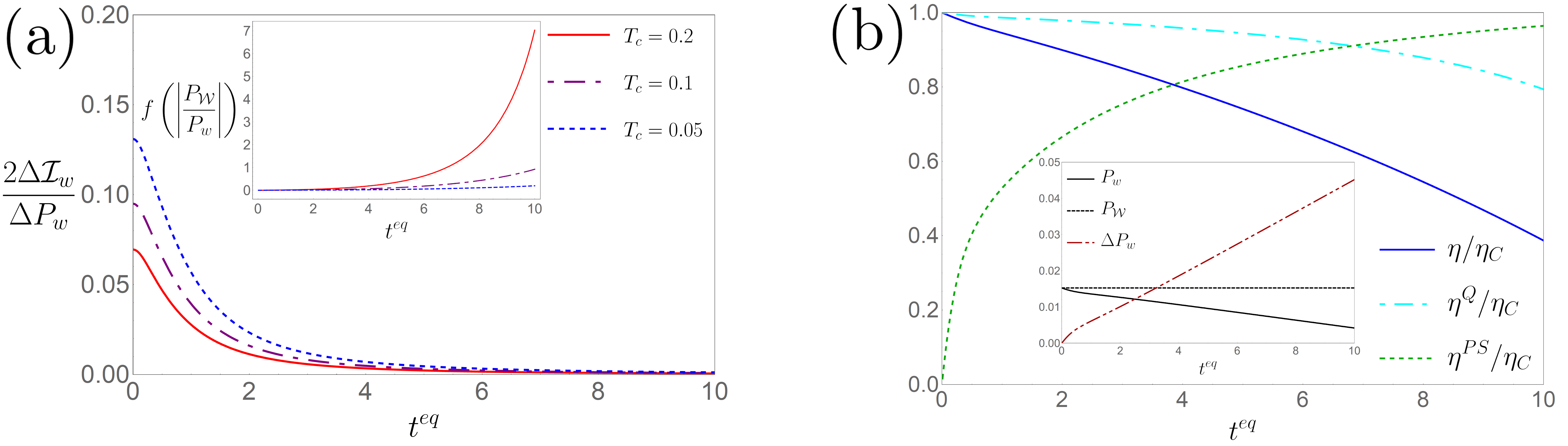
where and . Note that for the temperature, we have simply assigned in Eq.(3). This protocol is cyclic, , and satisfies the slow-driving condition for . In the Supplemental Material 22footnotemark: 2 we calculate the power and its fluctuations, as well as the efficiency and its bounds, using Eqs. (5), (9), and (11). Notably, the power operator does not commute with the engine Hamiltonian, , meaning that quantum friction is present throughout the cycle, and so the quantum correction term Eq.(12) is strictly positive. To see this effect, we plot the ratio between quantum and total power fluctuations, i.e. , in Fig. 1 (a). It can be seen how the quantum fluctuations become more relevant in the low temperature regime, , as expected. In this regime, the TUR Eq.(15) might become substantially affected by quantum fluctuations. Moreover, while the total power fluctuations vanish as (see the inset of Fig. 1 (b)), the ratio of the quantum fluctuations can be seen to increase as becomes smaller, showing that quantum fluctuations becomes more relevant in the slow-driving limit. Conversely, the correction term is large when is large, and vanishes in the limit . This means that, as can be seen in Fig. 1 (b), in the limit the engine produces finite power , while both the efficiency , as well as the bound given in Eq.(2), approaches Carnot. Finally, we see in Fig. 1 (b) that the bound in Eq.(1) does not apply to PDHEs; while the efficiency always obeys Eq.(2), it can violate Eq.(1) for sufficiently small , as this bound vanishes in the slow-driving limit, due to the fact that becomes vanishingly small.
Conclusions: We have derived a bound on the optimal efficiency of quantum periodically driven heat engines (PDHEs) in terms of their average power and constancy, valid in the slow-driving, Markovian regime. In the first instance, we see that PDHEs are subject to a bound that differs from steady-state heat engines (SSHEs) through an additional dependence on the ratio between adiabatic and actual power. Nonetheless, Eq.(2) still imposes a universal constraint on engine efficiency for a given power and constancy, thus providing a finite time correction to the Carnot bound at leading order in driving speed. The bound further incorporates the effect of quantum friction stemming from possibly non-commuting Hamiltonian driving. This represents the first Thermodynamic Uncertainty Relation for PDHEs that explicitly shows the role of quantum effects.
It has recently been shown that quantum friction reduces the maximum power achievable in slow driving PDHEs Brandner et al. (2017); Brandner and Saito (2020); Abiuso and Perarnau-Llobet (2020); Abiuso et al. (2020). Our results demonstrate that in this operational regime, quantum friction limits the efficiency relative to the subsequent reliability and power. More specifically, when optimising any one of the trio while fixing the other two variables, quantum friction inevitably leads to a reduction in the maximum value that can be attained. Given that enhancements with a quantum origin have been identified in other thermodynamic contexts, such as Otto-like engines Uzdin et al. (2015); Klatzow et al. (2019); Lostaglio (2020) or refrigerators Brunner et al. (2014), a full understanding of the role of quantum effects in PDHEs beyond the slow-driving and weak-coupling regime remain as open questions.
Acknowledgements.
Acknowledgements: H. J. D. M. acknowledges support from the Royal Commission for the Exhibition of 1851. M. H. M. acknowledges support from the Slovak Academy of Sciences under MoRePro project OPEQ (19MRP0027), as well as projects OPTIQUTE (APVV-18-0518) and HOQIT (VEGA 2/0161/19). M. P.-L. acknowledges funding from Swiss National Science Foundation (Ambizione PZ00P2-186067). G. G. acknowledges fundings from FQXi and DFG Grant No. FOR2724. G. G. also acknowledges funding from European Unions Horizon 2020 research and innovation programme under the Marie Sklodowska-Curie Grant Agreement No. 101026667.References
- Blickle and Bechinger (2012) V. Blickle and C. Bechinger, Nat. Phys. 8, 143 (2012).
- Pekola (2015) J. P. Pekola, Nat. Phys. 11, 118 (2015).
- Ronzani et al. (2018) A. Ronzani, B. Karimi, J. Senior, Y.-C. Chang, J. T. Peltonen, C. Chen, and J. P. Pekola, Nat. Phys. 14, 991 (2018).
- Benenti et al. (2017) G. Benenti, G. Casati, K. Saito, and R. S. Whitney, Phys. Rep. 1, 694 (2017).
- Brandner and Seifert (2016) K. Brandner and U. Seifert, Phys. Rev. E 93, 062134 (2016).
- Mohammady and Romito (2019) M. H. Mohammady and A. Romito, Phys. Rev. E 100, 012122 (2019).
- Seifert (2012) U. Seifert, Rep. Prog. Phys 75, 126001 (2012).
- Campisi et al. (2011) M. Campisi, P. Hänggi, and P. Talkner, Rev. Mod. Phys, 83, 771 (2011).
- Goold et al. (2016) J. Goold, M. Huber, A. Riera, L. del Rio, and P. Skrzypczyk, J. Phys. A 49, 143001 (2016).
- Pietzonka and Seifert (2018) P. Pietzonka and U. Seifert, Phys. Rev. Lett. 120, 190602 (2018).
- Gingrich et al. (2016) T. R. Gingrich, J. M. Horowitz, N. Perunov, and J. L. England, Phys. Rev. Lett. 116, 120601 (2016).
- Barato and Seifert (2015) A. C. Barato and U. Seifert, Phys. Rev. Lett. 114, 158101 (2015).
- Horowitz and Gingrich (2020) J. M. Horowitz and T. R. Gingrich, Nat. Phys. 16, 15 (2020).
- Guarnieri et al. (2019) G. Guarnieri, G. T. Landi, S. R. Clark, and J. Goold, Phys. Rev. Research 1, 033021 (2019).
- Macieszczak et al. (2018) K. Macieszczak, K. Brandner, and J. P. Garrahan, Phys. Rev. Lett. 121, 130601 (2018).
- Hasegawa (2020) Y. Hasegawa, Phys. Rev. Lett. 125, 050601 (2020).
- Hasegawa (2021) Y. Hasegawa, Phys. Rev. Lett. 126, 010602 (2021).
- Potts and Samuelsson (2019) P. P. Potts and P. Samuelsson, Phys. Rev. E 100, 052137 (2019).
- Barato and Seifert (2016) A. C. Barato and U. Seifert, Phys. Rev. X 6, 041053 (2016).
- Holubec and Ryabov (2018) V. Holubec and A. Ryabov, Phys. Rev. Lett. 121, 120601 (2018).
- Van Vu and Hasegawa (2020) T. Van Vu and Y. Hasegawa, Phys. Rev. Research 2, 013060 (2020).
- Cangemi et al. (2020) L. M. Cangemi, V. Cataudella, G. Benenti, M. Sassetti, and G. D. Filippis, Phys. Rev. B 102, 165418 (2020).
- Koyuk and Seifert (2020) T. Koyuk and U. Seifert, Phys. Rev. Lett. 125, 260604 (2020).
- Proesmans and Broeck (2017) K. Proesmans and C. V. D. Broeck, Euro. Phys Lett. 119, 20001 (2017).
- Proesmans and Horowitz (2019) K. Proesmans and J. M. Horowitz, J. Stat. Mech. 2019, 054005 (2019).
- Koyuk and Seifert (2019) T. Koyuk and U. Seifert, Phys. Rev. Lett. 122, 230601 (2019).
- Mandal and Jarzynski (2016) D. Mandal and C. Jarzynski, J. Stat. Mech. 2016, 063204 (2016).
- Feldmann and Kosloff (2003) T. Feldmann and R. Kosloff, Phys. Rev. E 68, 016101 (2003).
- Plastina et al. (2014) F. Plastina, A. Alecce, T. J. G. Apollaro, G. Falcone, G. Francica, F. Galve, N. L. Gullo, and R. Zambrini, Phys. Rev. Lett. 113, 260601 (2014).
- Francica et al. (2019) G. Francica, J. Goold, and F. Plastina, Phys. Rev. E 99, 042105 (2019).
- Dann and Kosloff (2020) R. Dann and R. Kosloff, N. J. Phys 22, 013055 (2020).
- Miller et al. (2019) H. J. D. Miller, M. Scandi, J. Anders, and M. Perarnau-Llobet, Phys. Rev. Lett. 123, 230603 (2019).
- Scandi et al. (2020) M. Scandi, H. J. D. Miller, J. Anders, and M. Perarnau-Llobet, Phys. Rev. Research 2, 023377 (2020).
- Albash et al. (2012) T. Albash, S. Boixo, and D. A. Lidar, N. J. Phys 14, 123016 (2012).
- Brandner et al. (2015) K. Brandner, K. Saito, and U. Seifert, Phys. Rev. X 5, 031019 (2015).
- Alicki and Lendi (1987) R. Alicki and K. Lendi, Quantum Dynamical Semigroups and Applications (Springer, 1987).
- Alicki (1976) R. Alicki, Rep. Math. Phys. 10, 249 (1976).
- Esposito and Van Den Broeck (2010) M. Esposito and C. Van Den Broeck, Phys. Rev. Lett. 104, 090601 (2010).
- Esposito and Van den Broeck (2010) M. Esposito and C. Van den Broeck, Phys. Rev. E 82, 011143 (2010).
- Cavina et al. (2017) V. Cavina, A. Mari, and V. Giovannetti, Phys. Rev. Lett. 119, 050601 (2017).
- Brandner and Saito (2020) K. Brandner and K. Saito, Phys. Rev. Lett. 124, 040602 (2020).
- Note (1) The intrinsic relaxation timescale of the system is determined by the inverse spectral gap of the Lindbladian.
- Note (2) See Supplemental Material [url] for mathematical derivations and further details behind the main results, which includes Refs Fagnola2007; Boullion1971; riechers2018spectral; Fagnola-harmonic-oscillator; Petz2014.
- Scandi and Perarnau-Llobet (2019) M. Scandi and M. Perarnau-Llobet, Quantum 3, 197 (2019).
- Abiuso and Perarnau-Llobet (2020) P. Abiuso and M. Perarnau-Llobet, Phys. Rev. Lett. 124, 110606 (2020).
- Horowitz (2012) J. M. Horowitz, Phys. Rev. E 85, 1 (2012).
- Horowitz and Parrondo (2013) J. M. Horowitz and J. M. R. Parrondo, N. J. Phys 15, 085028 (2013).
- Horowitz and Sagawa (2014) J. M. Horowitz and T. Sagawa, J. Stat. Phys. 156, 55 (2014).
- Manzano et al. (2015) G. Manzano, J. M. Horowitz, and J. M. R. Parrondo, Phys. Rev. E 92, 032129 (2015).
- Liu (2016) F. Liu, Phys. Rev. E 93, 012127 (2016).
- Liu and Xi (2016) F. Liu and J. Xi, Phys. Rev. E 94, 062133 (2016).
- Manzano et al. (2018) G. Manzano, J. M. Horowitz, and J. M. R. Parrondo, Phys. Rev. X 8, 31037 (2018).
- Elouard and Mohammady (2018) C. Elouard and M. H. Mohammady, in Thermodynamics in the quantum regime: Fundamental Aspects and New Directions, Fundamental Theories of Physics, Vol. 195, edited by F. Binder, L. A. Correa, C. Gogolin, J. Anders, and G. Adesso (Springer International Publishing, Cham, 2018) pp. 363–393.
- Mohammady et al. (2020) M. H. Mohammady, A. Auffèves, and J. Anders, Commun. Phys. 3, 89 (2020).
- Menczel and Brandner (2020) C. Menczel, Paul Flindt and K. Brandner, Phys. Rev. Research 2, 033449 (2020).
- Murch et al. (2013) K. W. Murch, S. J. Weber, C. Macklin, and I. Siddiqi, Nature 502, 211 (2013).
- Pekola et al. (2013) J. P. Pekola, P. Solinas, A. Shnirman, and D. V. Averin, N. J. Phys 15, 115006 (2013).
- Naghiloo et al. (2020) M. Naghiloo, D. Tan, P. M. Harrington, J. J. Alonso, E. Lutz, A. Romito, and K. W. Murch, Phys. Rev. Lett. 124, 110604 (2020).
- Talkner et al. (2007) P. Talkner, E. Lutz, and P. Hänggi, Phys. Rev. E 75, 050102 (2007).
- Esposito et al. (2009) M. Esposito, U. Harbola, and S. Mukamel, Rev. Mod. Phys. 81, 1665 (2009).
- Miller et al. (2020) H. J. D. Miller, M. H. Mohammady, M. Perarnau-Llobet, and G. Guarnieri, (2020), arXiv:2011.11589 .
- Denes Petz and Szabo (2009) Denes Petz and S. Szabo, Int. J. Math. , 1 (2009).
- Hansen (2008) F. Hansen, Proc. Natl. Acad. Sci. USA 105, 9909 (2008).
- Wigner and Yanase (1963) E. P. Wigner and M. M. Yanase, J. Phys. Chem. 15, 1084 (1963).
- Luo (2006) S. Luo, Phys. Rev. A 73, 022324 (2006).
- Marvian and Spekkens (2014) I. Marvian and R. W. Spekkens, Nat. Comm. 5, 3821 (2014).
- Shitara and Ueda (2016) T. Shitara and M. Ueda, Phys. Rev. A 94, 062316 (2016).
- Frérot and Roscilde (2016) I. Frérot and T. Roscilde, Phys. Rev. B 94, 075121 (2016).
- Feldmann et al. (1985) T. Feldmann, B. Andresen, A. Qi, and P. Salamon, J. Chem. Phys. 83, 5849 (1985).
- Sivak and Crooks (2012) D. A. Sivak and G. E. Crooks, Phys. Rev. L 108, 190602 (2012) (2012).
- Denzler and Lutz (2020) T. Denzler and E. Lutz, (2020), arXiv:2007.01034 .
- Roßnagel et al. (2015) J. Roßnagel, S. T. Dawkins, K. N. Tolazzi, O. Abah, E. Lutz, F. Schmidt-Kaler, and K. Singer, Science 352, 325 (2015).
- Brandner et al. (2017) K. Brandner, M. Bauer, and U. Seifert, Phys. Rev. Lett. 119, 170602 (2017).
- Abiuso et al. (2020) P. Abiuso, H. J. D. Miller, M. Perarnau-Llobet, and M. Scandi, Entropy 22, 1076 (2020).
- Uzdin et al. (2015) R. Uzdin, A. Levy, and R. Kosloff, Phys. Rev. X 5, 031044 (2015).
- Klatzow et al. (2019) J. Klatzow, J. N. Becker, P. M. Ledingham, C. Weinzetl, K. T. Kaczmarek, D. J. Saunders, J. Nunn, I. A. Walmsley, R. Uzdin, and E. Poem, Phys. Rev. Lett. 122, 110601 (2019).
- Lostaglio (2020) M. Lostaglio, Phys. Rev. Lett. 125, 230603 (2020).
- Brunner et al. (2014) N. Brunner, M. Huber, N. Linden, S. Popescu, R. Silva, and P. Skrzypczyk, Phys. Rev. E 89, 032115 (2014).