Spontaneous Breaking of $U(1)$ Symmetry in Coupled Complex SYK Models

Abstract

As shown in [1], two copies of the large $N$ Majorana SYK model can produce spontaneous breaking of a $Z_{2}$ symmetry when they are coupled by appropriate quartic terms. In this paper we similarly study two copies of the complex SYK model coupled by a quartic term preserving the $U(1)\times U(1)$ symmetry. We also present a tensor counterpart of this coupled model. When the coefficient $\alpha$ of the quartic term lies in a certain range, the coupled large $N$ theory is nearly conformal. We calculate the scaling dimensions of fermion bilinear operators as functions of $\alpha$. We show that the operator $c_{1i}^{\dagger}c_{2i}$, which is charged under the axial $U(1)$ symmetry, acquires a complex dimension outside of the line of fixed points. We derive the large $N$ Dyson-Schwinger equations and show that, outside the fixed line, this $U(1)$ symmetry is spontaneously broken at low temperatures because this operator acquires an expectation value. We support these findings by exact diagonalizations extrapolated to large $N$.

1 Introduction and summary

There has been a great deal of interest in the fermionic quantum mechanical models which are exactly solvable in the large $N$ limit because they are dominated by a special class of Feynman diagrams, which are called melonic [2]. Perhaps the simplest such model is the Majorana SYK model consisting of a large number of Majorana fermions with random quartic interactions [3, 4]. Quantum mechanical models of this type have non-random tensor counterparts [5, 6], which have continuous symmetry groups (for reviews of the melonic models see [7, 8, 9, 10, 11, 12, 13, 14]). Both the random and non-random quantum mechanical models are solvable via the same melonic Dyson-Schwinger (DS) equations [15, 16, 17, 18, 6, 4], which indicate that the model is nearly conformal. One can obtain richer dynamics when more than one Majorana SYK or tensor models are coupled [19, 20, 21, 1]. In particular, when two such models are coupled by certain quartic interactions with a coefficient $\alpha$, one finds a line of fixed points when $\alpha$ is positive, while a gapped $Z_{2}$ symmetry breaking phase appears when $\alpha$ is negative [1].

In this paper we make further progress in this direction by obtaining similar coupled models where a $U(1)$ symmetry is broken spontaneously in the large $N$ limit. Our starting point is the complex SYK model [22, 23, 24, 25] (see also the earlier work [26, 27]), which has a $U(1)$ global symmetry. When two such models are coupled together by a quartic interaction preserving the $U(1)\times U(1)$ symmetry,

$$H=\sum_{i,j,k,l=1}^{N}J_{ij,kl}\Big{(}c^{{\dagger}}_{1i}c^{{\dagger}}_{1j}c_{1k}c_{1l}+c^{{\dagger}}_{2i}c^{{\dagger}}_{2j}c_{2k}c_{2l}+8\alpha c^{{\dagger}}_{1i}c^{{\dagger}}_{2j}c_{2k}c_{1l}\Big{)}\ ,$$ (1.1)

we find that it is possible to break one of the $U(1)$ symmetries spontaneously. The phase where the $U(1)$ symmetry is broken by a VEV of operator $c_{1i}^{\dagger}c_{2i}$ is found for $\alpha<0$ and $\alpha>1$. In contrast with the breaking of discrete symmetry in the coupled Majorana SYK model [1], there is no gap in the full large $N$ spectrum due to the Nambu-Goldstone phenomenon. It manifests itself in splittings of order $1/N$ between the lowest states in different charge sectors. However, some specific charge sectors exhibit gaps of order $1$ above the ground state.

We also exhibit a tensor counterpart of the coupled random model (1.1) which consists of two coupled complex tensor models. The basic such model with $SU(N)^{2}\times O(N)\times U(1)$ symmetry was introduced in [6], and the two are coupled by an interaction which preserves the $SU(N)^{2}\times O(N)\times U(1)^{2}$ symmetry.

At the special coupling $\alpha=1/4$, the $U(1)\times U(1)$ symmetry is enhanced to $U(2)\sim U(1)\times SU(2)$, and the Hamiltonian (1.1) may be written compactly as

$$H_{U(2)}=\sum_{i,j,k,l=1}^{N}J_{ij,kl}c^{{\dagger}}_{\sigma i}c^{{\dagger}}_{\sigma^{\prime}j}c_{\sigma^{\prime}k}c_{\sigma l}\,,$$ (1.2)

where there is a sum over $\sigma,\sigma^{\prime}=1,2$. This is equal to the quartic term in the model of [28], which was argued to provide a description of quantum dots with irregular boundaries. In (1.2) the $U(1)$ is the usual charge symmetry, while the enhanced $SU(2)$ symmetry models the physical spin; we may think of $\sigma$ as labeling the two spin states, up and down.

We note that some results on spontaneous $U(1)$ symmetry breaking in models with random couplings have already appeared in the literature [29, 30, 31, 32, 33, 34, 35, 36]. For example, toy models of superconductivity introduced in [30, 31, 36] include random Yukawa interactions of fermion-phonon type.

Other recently introduced models [29, 32, 33] include random quartic couplings, as well as the non-random double-trace operator $OO^{\dagger}$, where $O$ is a ”Cooper pair operator” $O\sim c_{i\uparrow}c_{i\downarrow}$. The models we study in this paper are somehwat different, and they appear to be the first examples of manifestly melonic theories where the spontaneous breaking of $U(1)$ symmetry can be established through analysis of the exact large $N$ Dyson-Schwinger equations.

The structure of the paper is as follows. In section 2 we introduce some melonic models with $U(1)\times U(1)$ symmetry. They include a pair of coupled complex SYK models with Hamiltonian (1.1), as well as the tensor counterpart of this model with Hamiltonian (2.11). In section 3 we discuss the symmetric saddle point of the large $N$ effective action, as well as fluctuations around it. There is a range $0\leq\alpha\leq 1$ where the symmetric saddle point is stable, while outside this fixed line a fermion bilinear operator, $c_{1i}^{\dagger}c_{2i}$, acquires a complex scaling dimension. In section 4 we find a more general solution of the Dyson-Schwinger equations, which contains the off-diagonal Green’s function $G_{12}$. It is stable outside the fixed line and indicates that the operator $c_{1i}^{\dagger}c_{2i}$ acquires an expectation value. This phase of the theory is characterized by the exponential fall-off of Green’s functions at low temperatures. In section 5 we discuss the low-energy effective action in this phase and calculate the compressibility for the broken $U(1)$ degree of freedom. In section 6 we support some of these results by Exact Diagonalizations at accessible values of $N$. Extrapolating the ground state energies and compressibilities to large $N$, we obtain good agreement with some of the results obtained using the DS equations. In section 7 we present results for compressibilities at the special value $\alpha=1/4$ where the model has $U(2)$ symmetry. Some additional details can be found in the Appendices.

As we were about to submit this paper to arXiv, we noticed the new paper [37] by S. Sahoo et al. where the model (1.1) is also studied, with results similar to some of ours.

2 Melonic models with $U(1)\times U(1)$ symmetry

In this section we introduce some melonic models with quartic Hamiltonians, which possess $U(1)\times U(1)$ symmetry. The first model with Hamiltonian (1.1) consists of two copies of complex SYK model with a marginal $U(1)\times U(1)$ preserving interaction containing a dimensionless coupling, $\alpha$. We also formulate its tensor counterpart which has $SU(N)^{2}\times O(N)\times U(1)^{2}$ symmetry; it has the same Dyson-Schwinger equations as the random model.

2.1 Two coupled complex SYK models

Consider two sets of $N$ complex fermions, $c_{\sigma i}$, where $\sigma=1,2$ and $i=1,\ldots,N$:

$$\{c^{{\dagger}}_{\sigma i},c_{\sigma^{\prime}j}\}=\delta_{\sigma\sigma^{\prime}}\delta_{ij}\ .$$ (2.1)

The Hamiltonian coupling them is (1.1), where $J_{ij,kl}$ is the random Gaussian complex tensor with zero mean $\overline{J_{ij,kl}}=0$; it satisfies $J_{ij,kl}=J^{*}_{kl,ij}$ in order for the Hamiltonian to be Hermitian. We also assume anti-symmetry in the first and second pairs of indices: $J_{ij,kl}=-J_{ji,kl}=-J_{ij,lk}$. The variance is $\overline{|J_{ij,kl}|^{2}}=J^{2}/(2N)^{3}$.

So far the definition of the random tensor $J_{ij,kl}$ is incomplete. In fact, there is some freedom in its definition [38] even for the single complex SYK model. In this paper we will not use this freedom and will adopt the following minimal approach. We decompose $J_{ij,kl}$ as $J_{ij,kl}=\frac{1}{4}(T_{ij,kl}+T^{*}_{kl,ij})$, where $T_{ij,kl}$ is antisymmetric in the first and second pairs of indices and has no other symmetries. We then treat $T_{ij,kl}$ as $N^{2}(N-1)^{2}/4$ independent complex Gaussian random variables, so $\overline{T_{ij,kl}}=0$ and $\overline{|T_{ij,kl}|^{2}}=J^{2}/N^{3}$.

The Hamiltonian (1.1) has two $U(1)$ symmetries,

$$U(1)_{+}: \quad c_{1i}\to e^{i\phi_{+}}c_{1i},\quad c_{2i}\to e^{i\phi_{+}}c_{2i}\ ;$$

$$U(1)_{-}: \quad c_{1i}\to e^{i\phi_{-}}c_{1i},\quad c_{2i}\to e^{-i\phi_{-}}c_{2i}\ .$$ (2.2)

The corresponding conserved charges are $Q_{\pm}=Q_{1}\pm Q_{2}$ where

$$Q_{1}=\frac{1}{2}\sum_{i=1}^{N}[c^{{\dagger}}_{1i},c_{1i}]\ ,\qquad Q_{2}=\frac{1}{2}\sum_{i=1}^{N}[c^{{\dagger}}_{2i},c_{2i}]\ .$$ (2.3)

The allowed values of $Q_{1}$ and $Q_{2}$ are $-\frac{N}{2},-\frac{N}{2}+1,\ldots,\frac{N}{2}-1,\frac{N}{2}$; they are integer for even $N$ and half-integer for odd $N$. Both $Q_{+}$ and $Q_{-}$ take integer values ranging from $-N$ to $N$. Also, there are constraints that $Q_{+}+Q_{-}=2Q_{1}$ and $Q_{+}-Q_{-}=2Q_{2}$ are even for $N$ even and odd for $N$ odd.

The Hamiltonian also has the $Z_{4}$ symmetry

$$c_{1i}\rightarrow c_{2i}\ ,\qquad c_{2i}\rightarrow-c_{1i}\ ,$$ (2.4)

which is analogous to the $Z_{4}$ symmetry which played an important role in [1]. Another important symmetry is the particle-hole symmetry

$$c_{1i}\leftrightarrow c_{1i}^{\dagger}\ ,\qquad c_{2i}\leftrightarrow c_{2i}^{\dagger}\ ,\qquad J_{ij,kl}\rightarrow J^{*}_{ij,kl}\ .$$ (2.5)

In order to make the Hamiltonian invariant under this symmetry for general $\alpha$, we have to add to it certain quadratic and c-number terms which are exhibited in (A.4).

Note that, since the random coupling $J_{ij,kl}$ is complex, the $U(1)_{+}$ and $U(1)_{-}$ are on a different footing: the charge conjugation acting on the second flavor $c_{2i}$,

$$C_{2}^{\dagger}c_{2i}C_{2}=c_{2i}^{\dagger}$$ (2.6)

is not a symmetry of the Hamiltonian (1.1). The $U(1)_{+}$ is the overall charge symmetry, while the “axial” symmetry $U(1)_{-}$ may be thought of as a spatial rotation around the third axis. We will show that, for $\alpha<0$, the $U(1)_{-}$ may be broken spontaneously in the large $N$ limit, but the charge symmetry $U(1)_{+}$ remains unbroken. Holographically, the $U(1)_{-}$ has a simple physical meaning: a holographic state charged under $U(1)_{-}$ corresponds to bulk solutions with an electric field turned on.

Using the standard procedure for integrating over disorder and introducing bilocal fields,

$$G_{\sigma\sigma^{\prime}}(\tau_{1},\tau_{2})=\frac{1}{N}\langle Tc_{\sigma i}(\tau_{1})c_{\sigma^{\prime}i}^{\dagger}(\tau_{2})\rangle\ ,$$ (2.7)

and $\Sigma_{\sigma\sigma^{\prime}}(\tau_{1},\tau_{2})$, we write down the effective action

$$I=-\log\det(\delta^{\prime}(\tau_{12})\delta_{\sigma\sigma^{\prime}}-\Sigma_{\sigma\sigma^{\prime}}(\tau_{1},\tau_{2}))-\int d\tau_{1}d\tau_{2}\Sigma_{\sigma\sigma^{\prime}}(\tau_{1},\tau_{2})G_{\sigma^{\prime}\sigma}(\tau_{2},\tau_{1})-\frac{J^{2}}{4}\int d\tau_{1}d\tau_{2}V(G_{\sigma\sigma^{\prime}})\,,$$

$$V(G_{\sigma\sigma^{\prime}})=G_{11}^{2}(\tau_{1},\tau_{2})G_{11}^{2}(\tau_{2},\tau_{1})+G_{22}^{2}(\tau_{1},\tau_{2})G_{22}^{2}(\tau_{2},\tau_{1})+2G_{12}^{2}(\tau_{1},\tau_{2})G_{21}^{2}(\tau_{2},\tau_{1})$$

$$\qquad+16\alpha\big{(}G_{11}(\tau_{1},\tau_{2})G_{11}(\tau_{2},\tau_{1})+G_{22}(\tau_{1},\tau_{2})G_{22}(\tau_{2},\tau_{1})\big{)}G_{12}(\tau_{1},\tau_{2})G_{21}(\tau_{2},\tau_{1})+$$

$$\qquad+16\alpha^{2}\big{(}G_{11}(\tau_{1},\tau_{2})G_{22}(\tau_{1},\tau_{2})+G_{12}(\tau_{1},\tau_{2})G_{21}(\tau_{1},\tau_{2})\big{)}\big{(}G_{11}(\tau_{2},\tau_{1})G_{22}(\tau_{2},\tau_{1})+G_{12}(\tau_{2},\tau_{1})G_{21}(\tau_{2},\tau_{1})\big{)}\,.$$ (2.8)

For $\alpha=1/4$ this can be nicely written as

$$V(G_{\sigma\sigma^{\prime}})=\frac{1}{2}\textrm{Tr}\big{(}G(\tau_{1},\tau_{2})G(\tau_{2},\tau_{1})\big{)}^{2}+\frac{1}{2}\textrm{Tr}\big{(}G(\tau_{1},\tau_{2})G(\tau_{2},\tau_{1})G(\tau_{1},\tau_{2})G(\tau_{2},\tau_{1})\big{)}\,,$$ (2.9)

where $G(\tau_{1},\tau_{2})$ is a $2\times 2$ matrix with elements $G_{\sigma\sigma^{\prime}}(\tau_{1},\tau_{2})$. So we can clearly see that $V(G_{\sigma\sigma^{\prime}})$ is invariant under the global $U(2)$ transformations $G(\tau_{1},\tau_{2})\to U^{{\dagger}}G(\tau_{1},\tau_{2})U$.

2.2 Tensor counterpart of the random model

Let us recall that the tensor counterpart of the standard complex SYK model [23, 25] is given by the tensor model with Hamiltonian [6, 12]

$$h=g\bar{\psi}^{a_{1}b_{1}c_{1}}\bar{\psi}^{a_{2}b_{1}c_{2}}\psi^{a_{1}b_{2}c_{2}}\psi^{a_{2}b_{2}c_{1}}\ .$$ (2.10)

The tensor indices range from $1$ to $N$, so that the model contains $N^{3}$ fermions, and the dimension of its Hilbert space is $2^{N^{3}}$. The model has $SU(N)^{2}\times O(N)\times U(1)$ symmetry: the $O(N)$ symmetry acts on the second index of the tensor, while the two $SU(N)$ symmetries act on the first and third indices, respectively. Exchanging the two $SU(N)$ groups changes $h\to-h$.

Now we need to similarly determine the tensor counterpart of two coupled cSYK models (1.1). As we show in Appendix C, the same Dyson-Schwinger equations as for this random model follow from the coupled tensor model with $SU(N)^{2}\times O(N)\times U(1)^{2}$ symmetry, which has the Hamiltonian

$$H_{\rm tensor}=\frac{g}{2}\bigg{(} \bar{\psi}_{1}^{a_{1}b_{1}c_{1}}\bar{\psi}_{1}^{a_{2}b_{1}c_{2}}\psi_{1}^{a_{1}b_{2}c_{2}}\psi_{1}^{a_{2}b_{2}c_{1}}+\bar{\psi}_{2}^{a_{1}b_{1}c_{1}}\bar{\psi}_{2}^{a_{2}b_{1}c_{2}}\psi_{2}^{a_{1}b_{2}c_{2}}\psi_{2}^{a_{2}b_{2}c_{1}}$$

$$+ 4\alpha\left(\bar{\psi}_{1}^{a_{1}b_{1}c_{1}}\bar{\psi}_{2}^{a_{2}b_{1}c_{2}}\psi_{2}^{a_{1}b_{2}c_{2}}\psi_{1}^{a_{2}b_{2}c_{1}}-\bar{\psi}_{1}^{a_{1}b_{1}c_{1}}\bar{\psi}_{2}^{a_{2}b_{1}c_{2}}\psi_{2}^{a_{2}b_{2}c_{1}}\psi_{1}^{a_{1}b_{2}c_{2}}\right)\bigg{)}\ .$$ (2.11)

Under interchange of the two $SU(N)$ groups the Hamiltonian changes sign, and we have chosen the coupling term multiplied by $\alpha$ to preserve this discrete symmetry. The $U(1)\times U(1)$ symmetry acts analogously to that in the random model,

$$U(1)_{+}: \quad\psi_{1}^{abc}\to e^{i\phi_{+}}\psi_{1}^{abc},\qquad\psi_{2}^{abc}\to e^{i\phi_{+}}\psi_{2}^{abc}\ ;$$

$$U(1)_{-}: \quad\psi_{1}^{abc}\to e^{i\phi_{-}}\psi_{1}^{abc},\qquad\psi_{2}^{abc}\to e^{-i\phi_{-}}\psi_{2}^{abc}\ .$$ (2.12)

The Hamiltonian is also symmetric under the $\pi/2$ rotation $\psi_{1}^{abc}\rightarrow\psi_{2}^{abc}$, $\psi_{2}^{abc}\rightarrow-\psi_{1}^{abc}$.

In the tensor model (2.11) we may gauge the non-abelian symmetry $SU(N)^{2}\times O(N)$, restricting the states and operators to the sector invariant under this symmetry. Furthermore, as in the random counterpart (1.1), it is possible to gauge the $U(1)_{+}$ symmetry.

For $\alpha=1/4$, the symmetry is enhanced to $SU(N)^{2}\times O(N)\times U(2)$, and the Hamiltonian may be written as

$$H_{\rm tensor}=\frac{g}{4}\left(\bar{\psi}_{\sigma}^{a_{1}b_{1}c_{1}}\bar{\psi}_{\sigma^{\prime}}^{a_{2}b_{1}c_{2}}\psi_{\sigma^{\prime}}^{a_{1}b_{2}c_{2}}\psi_{\sigma}^{a_{2}b_{2}c_{1}}-\bar{\psi}_{\sigma}^{a_{1}b_{1}c_{1}}\bar{\psi}_{\sigma^{\prime}}^{a_{2}b_{1}c_{2}}\psi_{\sigma^{\prime}}^{a_{2}b_{2}c_{1}}\psi_{\sigma}^{a_{1}b_{2}c_{2}}\right)\ .$$ (2.13)

For $\alpha=0$, the Hamiltonian (2.11) becomes a sum of two Hamiltonians (2.10). In the tensor model (2.11) the gauged $SU(N)$ symmetries forbid correlators of the form $\langle\psi_{\sigma}^{abc}(t)\psi_{\sigma^{\prime}}^{a^{\prime}b^{\prime}c^{\prime}}(0)\rangle$, and the corresponding operators $\psi_{\sigma}^{abc}\partial_{t}^{m}\psi_{\sigma^{\prime}}^{abc}$ are not allowed (in the random model, these operators do not receive ladder corrections). The symmetries do allow correlators of the form $\bar{\psi}_{\sigma}^{abc}\partial_{t}^{m}\psi_{\sigma^{\prime}}^{abc}$, and their large $N$ scaling dimensions are non-trivial. We will determine their values as functions of $\alpha$ in the next section, and show that one of them is complex for $\alpha<0$ and $\alpha>1$.

3 Scaling Dimensions of Fermion Bilinears

First let us study the large $N$ saddle point where

$$G_{12}=G_{21}=0\,\quad\Sigma_{12}=\Sigma_{21}=0\,,$$ (3.1)

so that the $U(1)_{+}\times U(1)_{-}$ symmetry is preserved. Next it is reasonable to assume that $G_{11}(\tau_{1},\tau_{2})=G_{22}(\tau_{1},\tau_{2})=G(\tau_{12})$, where $G(\tau)$ is the particle-hole symmetric Green’s function, so $G(-\tau)=-G(\tau)$. And we obtain

$$\partial_{\tau}G(\tau)-\int d\tau^{\prime}\Sigma(\tau-\tau^{\prime})G(\tau^{\prime})=\delta(\tau)\,,$$

$$\Sigma(\tau)=J^{2}(1+8\alpha^{2})G^{3}(\tau)\,,$$ (3.2)

which is the standard SYK Dyson-Schwinger (DS) equations with $J^{\prime}=J\sqrt{1+8\alpha^{2}}$. We will see that this diagonal saddle point describes the theory in the range $0\leq\alpha\leq 1$, where various large $N$ quantities are related to those in the $\alpha=0$ theory by the rescaling of $J$. For example, the ground state energy is

$$E_{0}(\alpha)=2E_{0}^{\textrm{cSYK}}\sqrt{1+8\alpha^{2}}\approx-0.1624NJ\sqrt{1+8\alpha^{2}}\ .$$ (3.3)

Now we consider the bilinear spectrum at the nearly conformal saddle 3. They can be obtained by considering the melonic Bethe-Salpeter equations for the three point functions. Due to $U(1)_{+}\times U(1)_{-}$ symmetry, we can separate the computations in terms of

$$v_{\sigma\sigma^{\prime}}^{0,2(\sigma-\sigma^{\prime})}(\tau,0,\infty)=\langle c^{\dagger}_{\sigma i}(\tau)c_{\sigma^{\prime}i}(0)\mathcal{O}_{h}^{0,2(\sigma-\sigma^{\prime})}(\infty)\rangle\ ,$$ (3.4)

between elementary fermions $c_{\sigma i}^{\dagger},c_{\sigma^{\prime}i}$ and a primary operator $\mathcal{O}_{h}^{0,2(\sigma-\sigma^{\prime})}$ with dimension $h$ and $U(1)_{+}\times U(1)_{-}$ charge $(0,2(\sigma-\sigma^{\prime})).$ Note that operators with non-zero $U(1)_{+}$ charge do not receive ladder correction in the large $N$ limit due to $J_{ij,kl}$ being complex.

It is convenient to write down schematically the bilinear operators $\{\mathcal{O}_{m,+}^{0,0},\mathcal{O}^{0,0}_{m,-},\mathcal{O}_{m}^{0,2},\mathcal{O}_{m}^{0,-2}\}$:

$$\mathcal{O}^{0,0}_{m,\pm}=c_{1i}^{\dagger}\partial_{\tau}^{m}c_{1i}\pm c_{2i}^{\dagger}\partial_{\tau}^{m}c_{2i},\quad\mathcal{O}^{0,2}_{m}=c_{1i}^{\dagger}\partial_{\tau}^{m}c_{2i}+(-1)^{m+1}c_{2i}\partial_{\tau}^{m}c_{1i}^{\dagger},\quad\mathcal{O}_{m}^{0,-2}=c_{2i}^{\dagger}\partial_{\tau}^{m}c_{1i}+(-1)^{m+1}c_{1i}\partial_{\tau}^{m}c_{2i}^{\dagger}\ .$$ (3.5)

This simple form of operators applies to the free UV theory (for a more precise form of the conformal primary operators in the SYK model, see [39]), but in the interacting IR theory the operators have a more complicated form. We will now present a calculation of their scaling dimensions which is exact in the IR limit of the large $N$ theory.

For $(0,0)$ operators the scaling dimensions are determined by the following matrix:

$$K_{(0,0)}=\frac{1}{1+8\alpha^{2}}\begin{pmatrix}\frac{2}{3}K_{c}-\frac{1}{3}K_{c}^{T}+\frac{8\alpha^{2}}{3}K_{c}&\frac{8\alpha^{2}}{3}(K_{c}-K_{c}^{T})\\ \frac{8\alpha^{2}}{3}(K_{c}-K_{c}^{T})&\frac{2}{3}K_{c}-\frac{1}{3}K_{c}^{T}+\frac{8\alpha^{2}}{3}K_{c}\end{pmatrix},$$ (3.6)

where we define $K_{c}$ as the conformal kernel of a single SYK/tensor model with Majorana fermions:

$$K_{c}(\tau_{1},\tau_{2},\tau_{3},\tau_{4})=-\frac{3}{4\pi}\frac{\text{sgn}(\tau_{13})\text{sgn}(\tau_{24})}{|\tau_{13}|^{2\Delta}|\tau_{24}|^{2\Delta}|\tau_{34}|^{2-4\Delta}}\ ,\qquad\Delta=\frac{1}{4}\ .$$ (3.7)

which has eigenvalues in the anti-symmetric and symmetric sectors as $g_{a}(h),3g_{s}(h),$ with

$$g_{a}(h)=-\frac{3}{2}\frac{\tan(\frac{\pi}{2}(h-\frac{1}{2}))}{h-\frac{1}{2}}\ ,\qquad g_{s}(h)=-\frac{1}{2}\frac{\tan(\frac{\pi}{2}(h+\frac{1}{2}))}{h-\frac{1}{2}}\ ,$$ (3.8)

and $K_{c}^{T}(\tau_{1},\tau_{2},\tau_{3},\tau_{4})=K_{c}(\tau_{1},\tau_{2},\tau_{4},\tau_{3}).$

For the $(0,\pm 2)$ operators, they have the same anomalous dimensions determined by

$$K_{(0,\pm 2)}=\frac{8\alpha K_{c}-8\alpha^{2}K_{c}^{T}}{3(1+8\alpha^{2})}\,.$$ (3.9)

As a result, the scaling dimensions of the bilinear operators $\{\mathcal{O}_{m,+}^{0,0},\mathcal{O}^{0,0}_{m,-},\mathcal{O}_{m}^{0,2},\mathcal{O}_{m}^{0,-2}\}$ are determined by equating to $1$ the following functions:

$$\{g_{a}(h),\frac{3-8\alpha^{2}}{3(1+8\alpha^{2})}g_{a}(h),\frac{8\alpha(\alpha+1)}{3(1+8\alpha^{2})}g_{a}(h),\frac{8\alpha(\alpha+1)}{3(1+8\alpha^{2})}g_{a}(h)\}\quad m\text{ odd}\ ,$$

$$\{g_{s}(h),g_{s}(h),\frac{8\alpha(1-\alpha)}{1+8\alpha^{2}}g_{s}(h),\frac{8\alpha(1-\alpha)}{1+8\alpha^{2}}g_{s}(h)\}\quad m\text{ even}\ .$$ (3.10)

The series of scaling dimensions coming from solving $g_{a}(h)=1$ and $g_{s}(h)=1$ are the same as those found in a single complex SYK model or the $SU(N)^{2}\times O(N)\times U(1)$ tensor model [6]. Thus, for any $\alpha\neq\frac{1}{4}$, there are two $h=1$ modes corresponding to the $U(1)\times U(1)$ symmetry.

For $\alpha=\frac{1}{4}$, we find

$$\{g_{a}(h),\frac{5}{9}g_{a}(h),\frac{5}{9}g_{a}(h),\frac{5}{9}g_{a}(h)\},\quad\{g_{s}(h),g_{s}(h),g_{s}(h),g_{s}(h)\}\,.$$ (3.11)

Thus, four modes with $h=1$ are present. They are solutions with the smallest dimensions in their series and correspond to operators

$$c_{1i}^{\dagger}c_{1i}\pm c_{2i}^{\dagger}c_{2i},\qquad c_{1i}^{\dagger}c_{2i}\pm c_{2i}^{\dagger}c_{1i}\ ,$$ (3.12)

which are proportional to the generators of the $U(2)$ symmetry $\frac{1}{2}c_{\sigma i}^{{\dagger}}\lambda^{a}_{\sigma\sigma^{\prime}}c_{\sigma^{\prime}i}$.

ln contrast to the coupled Majorana SYK model [1], the large $N$ operator spectrum (3) does not exhibit a duality symmetry. A duality (4.7 can be explored at level of DS equations after assuming certain symmetries on the correlators, but fluctuations not obeying such symmetries prevent this duality from being exact. For example, the theory at $\alpha=1$ is not equivalent to that at $\alpha=0$. For $\alpha=1$, we note that the operator $\mathcal{O}^{0,0}_{1,-}=c_{1i}^{\dagger}\partial_{\tau}c_{1i}-c_{2i}^{\dagger}\partial_{\tau}c_{2i}$ has dimension $h\approx 1.2829$. Since this lies in the range $1<h<\frac{3}{2}$, the conformal solution might not be described by a Schwarzian theory [40]. In fact, $\mathcal{O}_{1,-}^{0,0}$ has scaling dimension in this range when $\alpha>\sqrt{\frac{3}{8}}$.

For $\alpha<0$ or $\alpha>1$ the nearly conformal phase becomes unstable because the scaling dimension of operators ${O}^{0,\pm 2}_{0}$ becomes complex. The plot of its imaginary part as a function of $\alpha$ is in fig. 1. We note that it reaches its maximum when $\alpha=-1/2.$ The antisymmetric sector cannot have such an instability for any $\alpha$ since $-1/3<\frac{3-8\alpha^{2}}{3(1+8\alpha^{2})}\leq 1$ and$-1/3<\frac{8\alpha(\alpha+1)}{3\left(1+8\alpha^{2}\right)}\leq 2/3$. So the lower bound is greater than $1/k_{a}(1/2)=-4/(3\pi)$. In such cases, the real infrared solution acquires VEV of ${O}^{0,\pm 2}_{0}$ corresponding to the spontaneous breaking of $U(1)_{-}$ symmetry.

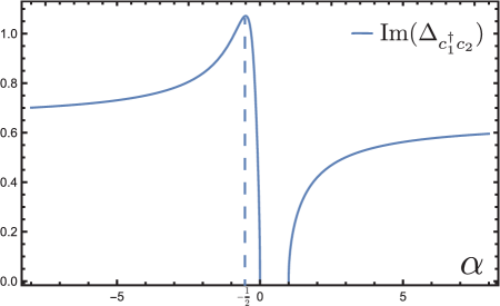
Figure 1: The imaginary part of the scaling dimension of operator $c^{\dagger}_{1i}c_{2i}$. It reaches its maximum at $\alpha=-1/2$.

4 General Dyson-Schwinger equations and their numerical solution

In this section we study the DS equations more generally and show that, for $\alpha<0$ or $\alpha>1$, the solution with lowest free energy breaks the $U(1)_{-}$ symmetry. These equations may be obtained by varying the effective action (2.8). The first series is

$$\partial_{\tau_{1}}G_{\sigma\sigma^{\prime}}(\tau_{1},\tau_{2})-\int d\tau_{3}\Sigma_{\sigma\sigma^{\prime\prime}}(\tau_{1},\tau_{3})G_{\sigma^{\prime\prime}\sigma^{\prime}}(\tau_{3},\tau_{2})=\delta_{\sigma\sigma^{\prime}}\delta(\tau_{12})\,.$$ (4.1)

For the second series we find

$$\Sigma_{11}(\tau_{12})= -J^{2}G_{11}(\tau_{12})^{2}G_{11}(\tau_{21})-4\alpha J^{2}G_{11}(\tau_{12})\big{(}G_{12}(\tau_{12})G_{21}(\tau_{21})+G_{12}(\tau_{21})G_{21}(\tau_{12})\big{)}$$

$$-8\alpha^{2}J^{2}G_{22}(\tau_{21})\big{(}G_{11}(\tau_{12})G_{22}(\tau_{12})+G_{12}(\tau_{12})G_{21}(\tau_{12})\big{)}\,,$$

$$\Sigma_{12}(\tau_{12})= -J^{2}G_{12}(\tau_{12})^{2}G_{21}(\tau_{21})-4\alpha J^{2}G_{12}(\tau_{12})\big{(}G_{11}(\tau_{12})G_{11}(\tau_{21})+G_{22}(\tau_{12})G_{22}(\tau_{21})\big{)}$$

$$-8\alpha^{2}J^{2}G_{12}(\tau_{21})\big{(}G_{11}(\tau_{12})G_{22}(\tau_{12})+G_{12}(\tau_{12})G_{21}(\tau_{12})\big{)}\ .$$ (4.2)

The equation for $\Sigma_{22}(\tau_{12})$ is obtained from $\Sigma_{11}(\tau_{12})$ by $G_{11}\leftrightarrow G_{22}$, and that for $\Sigma_{21}(\tau_{12})$ is obtained from $\Sigma_{12}(\tau_{12})$ by $G_{12}\leftrightarrow G_{21}$. In Appendix C we show how to derive these equations diagrammatically in both the coupled SYK and tensor models.

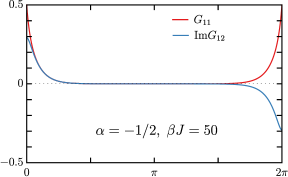
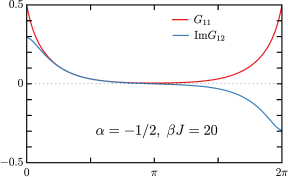
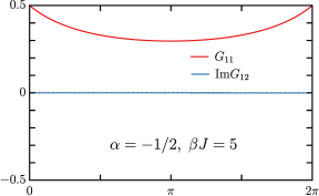
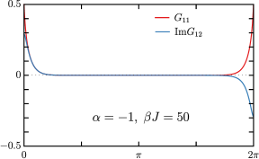
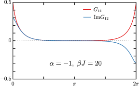
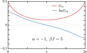
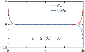
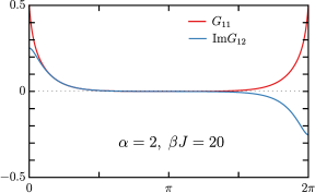
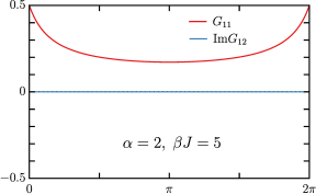
Figure 2: Numerical solutions to the DS equations for different values of $\alpha$ and $\beta J$, plotted against $\theta=\frac{2\pi\tau}{\beta}.$ All the values of $\alpha$ shown lie in the range where $U(1)_{-}$ is spontaneously broken at large $\beta J$. We note that all correlators exponentially decay at the same rate.

One can see that matrix $G_{\sigma\sigma^{\prime}}(\tau)$ is Hermitian $G^{{\dagger}}(\tau)=G(\tau)$, which implies that $G_{11}^{*}(\tau)=G_{11}(\tau)$ and $G_{12}^{*}(\tau)=G_{21}(\tau)$. The Particle-Hole symmetry implies that $G_{\sigma\sigma^{\prime}}(\tau)=-G_{\sigma^{\prime}\sigma}(-\tau)$, which leads to

$$G_{12}(-\tau)=-G_{21}(\tau)=-G_{12}^{*}(\tau)\ .$$ (4.3)

Assuming also that $G_{22}(\tau)=G_{11}(\tau)$, we find for the DS equations

$$J^{-2}\Sigma_{11}(\tau)= (1+8\alpha^{2})G_{11}(\tau)^{3}+4\alpha G_{11}(\tau)\big{(}G_{12}^{2}(\tau)+G_{12}^{*2}(\tau)+2\alpha|G_{12}(\tau)|^{2}\big{)}\,,$$

$$J^{-2}\Sigma_{12}(\tau)= G_{12}^{3}(\tau)+8\alpha G_{12}(\tau)G_{11}^{2}(\tau)+8\alpha^{2}G_{12}^{*}(\tau)(G_{11}^{2}(\tau)+|G_{12}(\tau)|^{2})\ ,$$ (4.4)

together with $\Sigma_{22}(\tau)=\Sigma_{11}(\tau)$ and $\Sigma_{21}(\tau)=\Sigma_{12}^{*}(\tau)$. We notice that $G_{11}(\tau)$ is real, $G_{11}^{*}(\tau)=G_{11}(\tau)$, whereas $G_{12}(\tau)$ can be complex. The first series of DS equations then reads

$$\partial_{\tau}G_{11}(\tau)-\int d\tau^{\prime}\big{(}\Sigma_{11}(\tau-\tau^{\prime})G_{11}(\tau^{\prime})+\Sigma_{12}(\tau-\tau^{\prime})G_{12}^{*}(\tau^{\prime})\big{)}=\delta(\tau)\,,$$

$$\partial_{\tau}G_{12}(\tau)-\int d\tau^{\prime}\big{(}\Sigma_{11}(\tau-\tau^{\prime})G_{12}(\tau^{\prime})+\Sigma_{12}(\tau-\tau^{\prime})G_{11}(\tau^{\prime})\big{)}=0\,.$$ (4.5)

Now we can look for solutions preserving different kinds of discrete symmetries. If we assume that the solution preserves the $Z_{4}$ symmetry (2.4), then we have $G_{12}(\tau)=-G_{21}(\tau)$. Combining this with $G_{12}^{*}(\tau)=G_{21}(\tau)$, we see that $G_{12}$ is purely imaginary. Using also (4.3), we find that $G_{12}(\tau)=G_{12}(-\tau)$. Therefore, similarly to [1], we have to solve for only two functions: an odd real one, $G_{11}(\tau)=G_{22}(\tau)$, and an even imaginary one, $G_{12}(\tau)$. The equations determining these two functions are

$$J^{-2}\Sigma_{11}(\tau)= (1+8\alpha^{2})G_{11}^{3}(\tau)+8\alpha(1-\alpha)G_{11}(\tau)G_{12}^{2}(\tau)\,,$$

$$J^{-2}\Sigma_{12}(\tau)= (1+8\alpha^{2})G_{12}^{3}(\tau)+8\alpha(1-\alpha)G_{12}(\tau)G_{11}^{2}(\tau)\ .$$ (4.6)

They are very similar to the equations derived in [1]; the functions of $\alpha$ are somewhat different, but they again demonstrate changes of behavior at $\alpha=0$ and $1$. The solutions to these equations may be obtained similarly to those in [1], and they are plotted in fig. 2.

We note that there is a duality symmetry of (4.6): these equations are invariant under

$$J\to\frac{1+8\alpha}{3}J\ ,\qquad\alpha\to\frac{1-\alpha}{1+8\alpha}\ .$$ (4.7)

However, this is not a symmetry of the theory even in the large $N$ limit: neither (4.4), nor the bilinear spectrum (3) respect it.

Due to the underlying $U(1)_{-}$ symmetry, there is a continuous family of solutions obtained from these ones through the transformation $G_{12}(\tau)\rightarrow e^{i\phi}G_{12}(\tau)$. If we don’t a priori assume the $Z_{4}$ symmetry (2.4), we find that the general numerical algorithm typically converges to a solution of this form with some phase $\phi$. We note that such a solution has a modified discrete symmetry $c_{1j}\rightarrow e^{-i\phi}c_{2j}$, $c_{2j}\rightarrow-e^{i\phi}c_{1j}$.

Let us calculate the expectation values of the $U(1)\times U(1)$ charges. After introducing a point splitting regulator and writing

$$Q_{1}=\lim_{\epsilon\rightarrow 0}\frac{1}{2}[c^{{\dagger}}_{1i}(\epsilon),c_{1i}(0)]\ ,$$ (4.8)

it follows that

$$\langle Q_{1}\rangle=\frac{1}{2}\lim_{\epsilon\rightarrow 0^{+}}\left(G_{11}(\epsilon)+G_{11}(-\epsilon)\right)=\frac{1}{2}\lim_{\epsilon\rightarrow 0^{+}}\left(G_{11}(\epsilon)-G_{11}(\beta-\epsilon)\right)\ .$$ (4.9)

Since for the solution in fig.2 $G_{11}(\tau)=G_{22}(\tau)$ has the symmetry $G_{11}(\tau)=G_{11}(\beta-\tau)$, we see that

$$\langle Q_{+}\rangle=\lim_{\epsilon\rightarrow 0}\frac{1}{2}\left(G_{11}(\epsilon)-G_{11}(\beta-\epsilon)+G_{22}(\epsilon)-G_{22}(\beta-\epsilon)\right)=0\ .$$ (4.10)

Analogously, we see that $\langle Q_{-}\rangle=0$. Since $U(1)_{+}$ is unbroken, $\langle Q_{+}\rangle=0$ indicates that any ground state must have $Q_{+}=0.$ For the broken symmetry $U(1)_{-}$, $\langle Q_{-}\rangle=0$ follows from the charge conjugation symmetry we imposed on the solution. To see this we note that, in the large $N$ limit, the ground state admits decomposition in the eigenstates of $Q_{-}$: $|0\rangle=\sum_{q_{-}}c_{q_{-}}|q_{-}\rangle.$ The charge conjugation symmetry implies that $c_{q_{-}}=c_{-q_{-}}$; therefore, $\langle Q_{-}\rangle=\sum_{q_{-}>0}q_{-}(c_{q_{-}}-c_{-q_{-}})=0.$

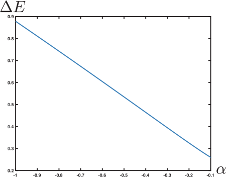
Figure 3: The gap $\Delta E$ (in units where $J=1$) for negative $\alpha$ calculated from the exponential decay of the solutions to the DS equations. We obtain the gap by linear fitting $\log|G_{11}|$ in regime $\frac{1}{J}\ll\tau\ll\beta,$ where the solution is dominated by the exponential decay, and the exponent is dominated by $\Delta E$ at zero temperature.

The exponential decay in fig. 2 indicates a $\mathcal{O}(1)$ gap at large $N$ between the ground state, which has $Q_{+}=0$, and the state with the lowest energy in the $Q_{+}=1$ sector, i.e.

$$\Delta E=E_{0}(Q_{+}=1)-E_{0}(Q_{+}=0)\ .$$ (4.11)

To see this, consider inserting a complete set of states

$$\langle c^{{\dagger}}_{\sigma}(\tau)c_{\sigma^{\prime}}(0)\rangle=\sum_{n}e^{(E_{0}-E_{n})\tau}\langle 0|c^{{\dagger}}_{\sigma}|n\rangle\langle n|c_{\sigma^{\prime}}|0\rangle\,,$$ (4.12)

where $\sigma,\sigma^{\prime}$ ranges from 1 to 2. In order for the matrix elements to be non-vanishing, $|n\rangle$ must have $Q_{+}=1.$ Using the numerical solutions to DS equations, extrapolated to large $\beta J$, we have plotted in fig. 3 the quantity $\Delta E$ from (4.11).

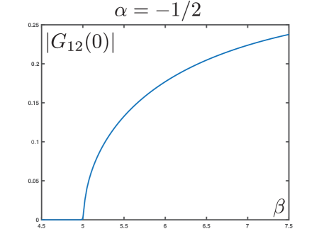
Figure 4: The magnitude of the off diagonal correlator at $\tau=0$, corresponding to the VEV of the operator ${c}_{1i}c_{2i}^{\dagger}$, plotted as a function of $\beta$ (we use units where $J=1$). A similar symmetry breaking behavior is observed for other values $\alpha<0$ or $\alpha>1$.

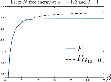
Figure 5: Numerical calculation of the large $N$ free energy and entropy at $\alpha=-\frac{1}{2}.$ Similarly to [1], for fixed $\alpha$ we observe a second-order phase transition from the $U(1)$ symmetric phase to $U(1)$ broken phase. We numerically observe that $S/N$ approaches zero, rather than a finite number, as $\beta\to\infty.$ This may be explained by the $U(1)$ sigma model, where one expects $S_{0}\sim\log N$ instead of powers in $N.$

Given the DS solution, we can also calculate the ground state energy via

$$\langle 0|H|0\rangle=\lim_{\epsilon\to 0^{+}}\frac{1}{2}\left(\langle c^{\dagger}_{1i}(\tau+\epsilon)\partial_{\tau}c_{1i}(\tau)\rangle+\langle c^{\dagger}_{2i}(\tau+\epsilon)\partial_{\tau}c_{2i}(\tau)\rangle\right)=\lim_{\tau\to 0^{+}}\partial_{\tau}G(\tau).$$ (4.13)

In momentum space this is given by

$$E_{0}=\frac{1}{\beta}\sum_{n}(\Sigma_{11}(\omega_{n})G_{11}(\omega_{n})-\Sigma_{12}(\omega_{n})G_{12}(\omega_{n}))\ .$$ (4.14)

We find good agreement between the DS computation of the ground state energy and the exact diagonalization results, as summarized in fig. 11.

5 Charge compressibility and the sigma model

Since the $U(1)_{-}$ symmetry is spontaneously broken for $\alpha<0$ and $\alpha>1$, we expect the presence of a gapless Goldstone mode. It arises from the degeneracy between ground states in sectors with different values of the charge $Q_{-}$, which emerges in the large $N$ limit. The expected action for the Goldstone modes is the $U(1)$ sigma model action:

$$S_{U(1)_{-}}=\frac{NK_{-}}{2}\int d\tau\ (\partial_{\tau}\phi(\tau))^{2}\,,\quad\phi\sim\phi+2\pi\ ,$$ (5.1)

where the coefficient $K_{-}$, which is $\mathcal{O}(1)$ in the large $N$ limit, is the zero-temperature compressibility for the $U(1)_{-}$ charge.

Let us emphasize that this $U(1)_{-}$ sigma model has a completely different origin from the $U(1)$ sigma model arising in the complex SYK model, which was recently discussed in detail in [25]. In the latter case, the physics is similar to the conventional SYK model: there is an approximate conformal symmetry in the IR, the Schwartzian effective action, zero-temperature entropy and, most importantly, U(1) symmetry is not broken. The $U(1)$ effective action for the complex SYK model [25] has the same origin as the Schwartzian action, since dropping the fermionic kinetic term promotes the global $U(1)$ symmetry to local $U(1)$. The finite $1/J$ corrections manifest themselves in the time-reparametrization Schwartzian mode and the $U(1)$-phase reparametrization sigma-model.

Assuming that in the range $0<\alpha<1$ the solution is given by the standard near-conformal SYK saddle, so there are no anomalous VEVs, we essentially have two non-interacting complex fermions. In particular, when chemical potential $\mu_{+}\neq 0$, the system has solution $G_{11}(\tau)=G_{22}(\tau),$ and when $\mu_{-}\neq 0,$ $G_{11}(\tau)=G_{22}(\beta-\tau).$ Both reduce (4.1) and (4) to that of two decoupled complex fermions with chemical potentials $\mu_{\pm}$. We then find that we have two sigma-models, for $U(1)_{\pm}$, with compressibilities:

$$K_{-}=K_{+}=\frac{2K_{\textrm{cSYK}}}{\sqrt{1+8\alpha^{2}}}\ ,$$ (5.2)

where $K_{cSYK}\approx 1.04$ is the compressibility of a single complex SYK model [25]. The factor of two comes from having two fermions, and the square root comes from renormalization of $J$ by non-zero $\alpha$, (3). Let us point out though that, at $\alpha=1/4$, the $U(1)_{-}$ symmetry is enhanced to $SU(2)$. We will discuss this case separately in section 7.

In the case of spontaneously broken $U(1)_{-}$ symmetry, the physics is different. The solutions of the Dyson-Schwinger equations that we have found for $\alpha<0$ do not have a conformal form. Therefore, there is no approximate reparametrization symmetry or Schwartzian effective action. In the large $N$ limit, the action (5.1) is a conventional Nambu-Goldstone mode action. On these grounds, we do not expect to have a sigma model for $U(1)_{+}$ symmetry, since it is unbroken. Therefore, the splittings between sectors with different values of $Q_{+}$ should not vanish in the large $N$ limit. This implies that the compressibility $K_{+}$ defined as $dQ_{+}/d\mu_{+}$ is zero, so that a small chemical potential does not generate non-zero charge. We will see this in the large $N$ DS equations momentarily. In the exact diagonalization at finite $N$, this manifests in the fact that the energy dependence on $Q_{+}$ is not close to quadratic.

Let us return to the $U(1)_{-}$ symmetry and compute the corresponding compressibility $K_{-}$. It can be found in three ways: First of all, it is the derivative of the charge with respect to the chemical potential:

$$K_{-}=\frac{dQ_{-}}{d\mu_{-}}\,,\quad\text{at}\ T=0\,,\mu_{-}=0\,.$$ (5.3)

Secondly, it is related to the grand canonical thermodynamical potential $\Omega$ as

$$\Omega=\Omega_{0}-\frac{NK_{-}\mu_{-}^{2}}{2}\,,\quad T=0\,,$$ (5.4)

and finally the action (5.1) can be quantized leading to the spectrum:

$$E_{Q_{-}}=A+\frac{Q_{-}^{2}}{2NK_{-}}\,,\quad Q_{-}\in\mathbb{Z}\,.$$ (5.5)

Let us emphasize that the $U(1)_{-}$ symmetry breaking occurs only in the limit $N\rightarrow\infty$. In systems with finite numbers of degrees of freedom this does not happen. From the above spectrum we see how it happens: if $N=\infty$ we have a classical particle on a circle (5.1) with an infinite number of classical vacua. However, finite $N$ effects quantize the action, leading to a unique ground state and spectrum (5.5).

It will be convenient for us to find $K_{-}$ numerically by introducing a chemical potential into the large $N$ Dyson-Schwinger equations and fitting the numerical result for $\Omega$ using eq. (5.4). In fact, to double check our results, we will introduce chemical potentials $\mu_{-}$ and $\mu_{+}$ for $U(1)_{-}$ and $U(1)_{+}$ and fit $\Omega$ with

$$\Omega=\Omega_{0}-\frac{NK_{-}\mu^{2}_{-}}{2}-\frac{NK_{+}\mu_{+}^{2}}{2}-NK_{\rm mix}\mu_{-}\mu_{+}\,.$$ (5.6)

Since $U(1)_{+}$ is unbroken, we expect that $K_{+}=K_{\text{mix}}=0$. In other words, the low energy states are not charged under $U(1)_{+}$, and the gap to states with non-vanishing $U(1)_{+}$ charges is big. The result is presented in Figure 6. We indeed see that $K_{+}=K_{\rm mix}=0$.

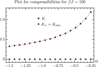
Figure 6: The numerical results for three different compressibilities as functions of $\alpha$ for $J=1$, $\beta=100$. We checked that the result does not depend appreciably on $\beta$ by comparing with the $\beta=50$ data.

Finally, we illustrate our claims by plotting the Green function $G_{11}$ upon introducing $\mu_{\pm}$ in fig. 7. These results were obtained by solving the DS equations numerically with $J=1,\beta=40,\alpha=-1.5$ and $\mu_{\pm}=0.3$. The expectation value of the charge $Q_{1}$ may be read off from the plot of $G_{11}$ using (4.9), and the expectation value of $Q_{2}$ is analogously determined by $G_{22}$.

From fig. 7 we observe that, when $\mu_{+}$ is turned on, the expectation values of $Q_{1}$ and $Q_{2}$ vanish despite the fact that the Green functions become asymmetric around $\pi$. This means that the expectation values of $Q_{\pm}=Q_{1}\pm Q_{2}$ vanish as well. On the other hand, when $\mu_{-}$ is turned on, the asymmetry in the values of $G_{11}$ at $0+$ and $2\pi-$ is clearly seen; the $G_{22}$ has the opposite asymmetry. Therefore, we now find that $\langle Q_{1}\rangle=-\langle Q_{2}\rangle\neq 0$, so that $\langle Q_{-}\rangle$ is non-vanishing.

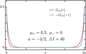
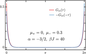
Figure 7: Plots of the Green functions when chemical potentials are turned on. For $\mu_{+}\neq 0$, $G_{22}(\tau)=G_{11}(\tau)$, while for $\mu_{-}\neq 0$, $G_{22}(\tau)=-G_{11}(-\tau)$. It follows that $\langle Q_{-}\rangle$ is generated for $\mu_{-}\neq 0$.

6 Results from Exact Diagonalizations

In this section we will study the energy spectra for accessible values of $N$. We will use the particle-hole symmetric version of the Hamiltonian, given in (A.4). We have generated multiple random samples of the Hamiltonain, which allow us to study various averaged quantities as functions of $\alpha$ and $N$.

6.1 Evidence for Symmetry Breaking

For $\alpha<0$ and $\alpha>1$, the large $N$ DS equations indicate that $U(1)_{-}$ symmetry is spontaneously broken. In these ranges of $\alpha$, the absolute ground state appears in the sectors with $Q_{+}=0$ and the lowest possible value of $|Q_{-}|$, which is $|Q_{-}|=0$ for even $N$ and $|Q_{-}|=1$ for odd $N$. This means that, for odd $N$, there are two degenerate ground states, which have $Q_{-}=\pm 1$, and their mixture admits an expectation value of operator $c_{1i}^{\dagger}c_{2i}$ already at finite $N$. At any finite even $N$ we cannot see the spontaneous symmetry breaking, but it appears in the large $N$ limit due to the degeneracy of ground states with $Q_{+}=0$ and different values of $Q_{-}$.

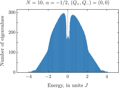
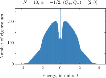
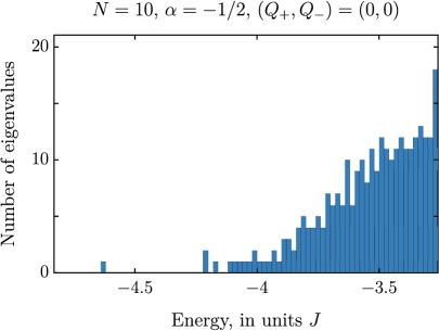
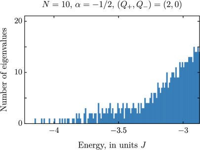
Figure 8: Density of states in two of the charge sectors, $(Q_{+},Q_{-})=(0,0)$ and $(2,0)$, for a single realization of the model with $N=10$ and $\alpha=-1/2$. The lower plots are zoomed in regions near the ground state. We observe a prominent gap in the $(Q_{+},Q_{-})=(0,0)$ sector.

In fig. 8 we exhibit the spectra in two different charge sectors for $N=10$. A characteristic quantity in the broken symmetry phase is the gap between the first excited state and the ground state: such a gap is observed in the sectors with $Q_{+}=0$. For example, in the $(Q_{+},Q_{-})=(0,1)$ sectors we find for $\alpha=-1/2$ that the average gaps above the ground state are $\approx 0.440,0.437,0.473$ for $N=7,9,11$, respectively. These results suggest that the gap is non-vanishing in the large $N$ limit.

Similarly, there is a sizable difference between the ground state energies in sectors with different values of $Q_{+}$. It is noticeably bigger than the difference between sectors with different values of $Q_{-}$, which is expected to be of order $1/N$. For example, for $\alpha=-1/2$ and $N=10$, we find

$$E_{0}(Q_{+}=2,Q_{-}=0)-E_{0}(Q_{+}=0,Q_{-}=0)\approx 0.622\ ,$$

$$E_{0}(Q_{+}=0,Q_{-}=2)-E_{0}(Q_{+}=0,Q_{-}=0)\approx 0.236\ .$$ (6.1)

In the sectors with $Q_{+}=0$, we expect the ground state energies to depend quadratically on $Q_{-}$:

$$E_{0}=A(\alpha,N)+\frac{Q_{-}^{2}}{2B_{-}(\alpha,N)}\ ,\qquad B_{-}(\alpha,N)=K_{-}(\alpha)N+C_{-}(\alpha)+O(1/N)\ ,$$ (6.2)

where $K_{-}$ is the large $N$ compressibility for the $U(1)_{-}$ degree of freedom. As can be seen in figs. 9 and 10, these quadratic fits work well, and $B_{-}(\alpha)$ is approximately linear in $N$.

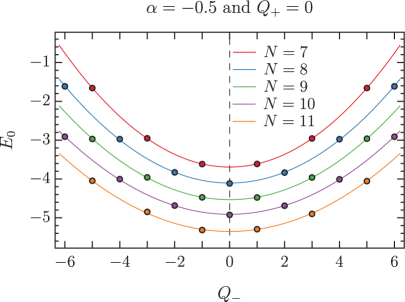
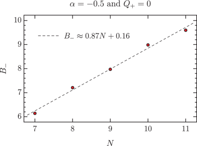
Figure 9: The $E(Q)$ curve(left) at $\alpha=-1/2$ for the first few $Q_{-}$ sectors at $Q_{+}=0.$ For each $E(Q)$ curve, we make a quadratic fit $E_{0}=\frac{Q_{-}^{2}}{2B_{-}}+A$ and determine $K_{-}$ from the linear fit of $B_{-}$ vs. $N$. The slope of the plot for $\alpha=-1/2$ is $K_{-}^{\textrm{ED}}\approx 0.87$, which agrees well with the DS calculation of $K_{-}^{\textrm{DS}}\approx 0.80$.

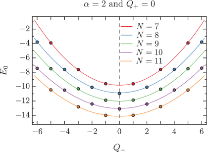
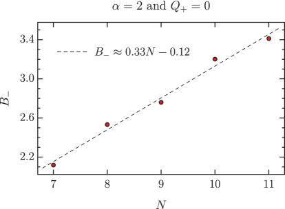
Figure 10: The $E(Q)$ curve(left) at $\alpha=2$ for the first few $Q_{-}$ sectors at $Q_{+}=0.$ The slope of the plot of $B_{-}$ vs. $N$ is $K_{-}^{\textrm{ED}}\approx 0.33$, which is not far from the DS calculation of $K_{-}^{\textrm{DS}}\approx 0.32$.

From the slopes we find that $K^{\textrm{ED}}_{-}(-0.5)\approx 0.87$ and $K^{\textrm{ED}}_{-}(2)\approx 0.33$. These values of compressibility are close to those obtained from the Dyson-Schwinger calculations directly in the large $N$ limit: $K^{\textrm{DS}}_{-}(-0.5)\approx 0.80$ and $K^{\textrm{DS}}_{-}(2)\approx 0.32$.

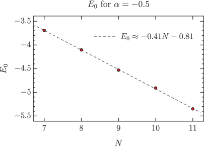
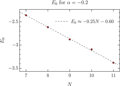
Figure 11: Plots of the leading term in the ground state energy (6.2), $A(\alpha,N)$, vs. $N$ for $\alpha=-0.5$ (left) and $\alpha=-0.2$ (right). The linear fits determining the slope, ${\cal E}_{0}(\alpha)$, are also shown.

Another important quantity is the leading term in the ground state energy (6.2), $A(\alpha,N)$, which is expected to grow linearly for large $N$. In fig. 11 we plot $A(\alpha,N)$ for $\alpha=-0.5$ and $\alpha=-0.2$, and show the fits

$$A(\alpha,N)={\cal E}_{0}(\alpha)N+D(\alpha)+O(1/N)\ .$$ (6.3)

In fig, 12 we plot ${\cal E}_{0}(\alpha)=\lim_{N\rightarrow\infty}E_{0}(\alpha)/N$ for a range of negative $\alpha$. This shows good agreement with the corresponding calculation using DS equation as a function of $\alpha$.

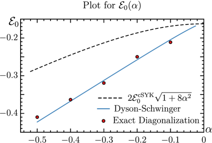
Figure 12: Comparison of the ED and DS calculations of ${\cal E}_{0}(\alpha)=\lim_{N\rightarrow\infty}E_{0}(\alpha)/N$. They show good agreement even though the ED results are available only up to a moderate values of $N$.

6.2 Line of Fixed Points

Along the fixed line $0\leq\alpha\leq 1$ there is no symmetry breaking, and the large $N$ spectrum is gapless in every charge sector. In fact, for such values of $\alpha,$ near the edge the density of state should behave as

$$\rho_{2\text{cSYK}}(E)=\int dE^{\prime}\rho_{\text{cSYK}}(E-E^{\prime})\rho_{\text{cSYK}}(E^{\prime})\sim E^{2}.$$ (6.4)

Along the fixed line, we expect the gaps to be of order $1/N$ for excitations of both the $Q_{-}$ and $Q_{+}$ charges, so that both $U(1)_{-}$ and $U(1)_{+}$ compressibilities are well-defined:

$$E_{0}=A(\alpha)+\frac{Q_{-}^{2}}{2B_{-}(\alpha,N)}+\frac{Q_{+}^{2}}{2B_{+}(\alpha,N)}\ ,$$

$$B_{\pm}(\alpha,N)=K_{\pm}(\alpha)N+C_{\pm}(\alpha)+O(1/N)\ .$$ (6.5)

For $0<\alpha<1$, we find that $B_{+}>B_{-}$ for all the values of $N$ we have studied. This leads to the fact that, for odd $N$, the ground state does not have $Q_{+}=0$. Indeed, for odd $N$, the lowest possible values of $(Q_{+},Q_{-})$ are $(0,\pm 1)$ and $(\pm 1,0)$. Since $B_{+}>B_{-}$, there are two ground states with $Q_{+}=\pm 1,Q_{-}=0$ for odd $N$. On the other hand, for even $N$ there is a unique ground state with $Q_{+}=Q_{-}=0$.

For $\alpha=0$, $B_{-}=B_{+}$. Therefore, the compressibilities are equal: $K_{+}(0)\approx K_{-}(0)\approx 2.08$. Indeed, for $\alpha=0$ the Hamiltonian is simply a sum of two cSYK Hamiltonian with the common $J_{ijkl}$, so that for large $N$

$$E_{0}=A(0)+\frac{1}{2NK_{\textrm{cSYK}}}\left(Q_{1}^{2}+Q_{2}^{2}\right)\ .$$ (6.6)

To compare with our normalizations, $K_{\textrm{cSYK}}=K_{+}(0)/2\approx 1.04$. Thus, our finding for $\alpha=0$ is in good agreement with the result $K_{\textrm{cSYK}}\approx 1$ from [25].

We have also done fits of the two large $N$ compressibilities along the fixed line. Then $K_{-}$ is found to be smaller than $K_{+}$. This is in conflict with the DS calculations giving equal values, which may be due to the slow convergence of the ED results to the large $N$ limit. The DS formula $K_{+}(\alpha)=K_{+}(0)/\sqrt{1+8\alpha^{2}}$ predicts the value $\approx 1.96$ at $\alpha=0.125$, and $\approx 0.94$ at $\alpha=0.7$. If we a priori assume $K_{-}=K_{+}=K(ED)$ in the ED fit for $\alpha>0,$ we obtain results in quite good agreement with the DS calculations. For example, at $\alpha=\frac{1}{8}$, $K(ED)\approx 1.92$ vs $K(DS)\approx 1.96.$ At $\alpha=0.7,$ we get $K(ED)\approx 0.95$ vs $K(DS)\approx 0.94.$

7 The $U(2)$ symmetric model

A special case is $\alpha=1/4$ where the Hamiltonian becomes (1.2), and the symmetry is enhanced to $SU(2)\times U(1)_{+}$. In this section we assemble various results at this special point, which is interesting because it corresponds to an SYK-like model with a non-abelian global symmetry [41, 42, 43, 44].

Due to the $SU(2)$ symmetry, there are some exact degeneracies in the spectrum between states with different values of $Q_{-}=2S_{z}$. The states naturally split into sectors labeled by the $U(1)_{+}$ charge $Q_{+}$ and the $SU(2)$ spin $S$. In fig. 13 we show the histogram for the $U(2)$ invariant states, which have $Q_{+}=S=0$. Such states appear only when $N$ is even, and the unique absolute ground state is in this sector. The histogram was obtained from a single realization of the Hamiltonian (A.4) with $N=10$, and it shows that the $U(2)$ symmetric theory is in the gapless phase.

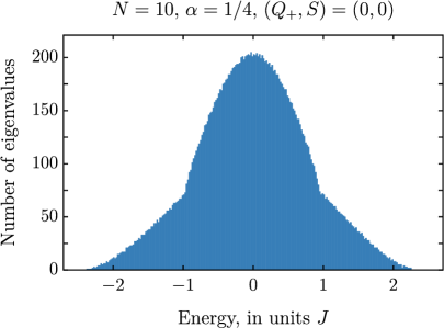
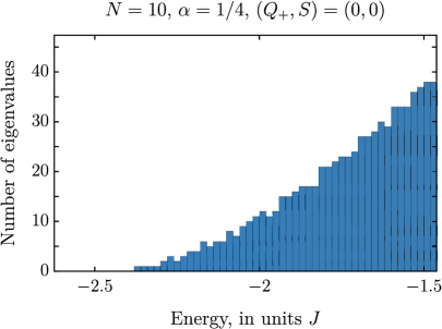
Figure 13: Density of states in the $(Q_{+},S)=(0,0)$ sector for a single realization at the $U(2)$ symmetric point $\alpha=\frac{1}{4}$ for $N=10$. The ground state is in this $U(2)$ invariant sector. On the right we enlarge the region near the ground state; this shows that there is no significant gap.

Let us discuss the low-energy effective action for the $U(2)$ symmetric theory. We expect that instead, of the $U(1)_{+}\times U(1)_{-}$ sigma model, we now have $SU(2)\times U(1)_{+}$. The low energy effective action for the $SU(2)$ part is:

$$S_{\textrm{SU(2)}}=-\frac{B_{\textrm{SU(2)}}}{4}\int d\tau{\operatorname{Tr}}\left(U^{\dagger}\partial_{\tau}U\right)^{2}\ ,$$

$$B_{\textrm{SU(2)}}=NK_{\textrm{SU(2)}}+C_{\textrm{SU(2)}}+O(1/N)\ ,$$ (7.1)

where $U(\tau)$ is a $SU(2)$ matrix variable. Previously, we obtained compressibilities from coupling to $\mu_{-}$ chemical potential. Let us argue that this calculation does not change. Indeed, corrections $\propto N$ to the free energy depend on classical properties of this sigma-model, since we have a factor of $N$ in front. Upon introducing a chemical potential for the $U(1)_{-}$ subgroup of $SU(2)$, we have to study the following action:

$$-\frac{B_{\textrm{SU(2)}}}{4}\int d\tau{\operatorname{Tr}}\left(U^{\dagger}\partial_{t}U+\mathop{\rm diag}\nolimits(\mu_{-},-\mu_{-})\right)^{2}\ .$$ (7.2)

Its contribution to the Gibbs potential is again $-B_{\textrm{SU(2)}}\mu_{-}^{2}/2$. We find using the DS equations that

$$K_{\textrm{SU(2)}}\approx 1.7\ .$$ (7.3)

However, the low energy spectrum is very different, as it involves quantizing the sigma model. Namely, now the excitations come in $SU(2)$ multiplets with energies given by a quadratic Casimir of $SU(2)$. Namely, for a multiplet with $Q_{-}/2\in(-S,-S+1,\dots,S)$ the energy is given by:

$$\delta E=\frac{2S(S+1)}{NK_{\textrm{SU(2)}}+C_{\textrm{SU(2)}}}\ .$$ (7.4)

Therefore, we find for large $N$:

$$E_{0}\approx A+\frac{1}{2(NK_{+}+C_{+})}Q_{+}^{2}+\frac{2}{NK_{\textrm{SU(2)}}+C_{\textrm{SU(2)}}}S(S+1)\ ,$$ (7.5)

where $S$ is the $SU(2)$ spin. For even $N$, the unique ground state occurs in the $Q_{+}=S=0$. For odd $N$, there are two ground states: they are $SU(2)$ singlets and have $Q_{+}=\pm 1$.

A priori, there are two different compressibilities; see fig. 14. Fitting them separately, we find $K_{\textrm{SU(2)}}\approx 1.45$ and $K_{+}\approx 1.78$. The fact that they are different disagrees with the DS results; this could be due to the fact that our data does not access large enough $N$. However, if we assume that they are equal, then the fit value is $K_{+}=K_{\textrm{SU(2)}}\approx 1.6$, which is not far from the DS value (7.3).

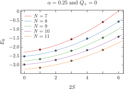
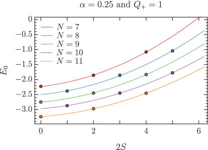
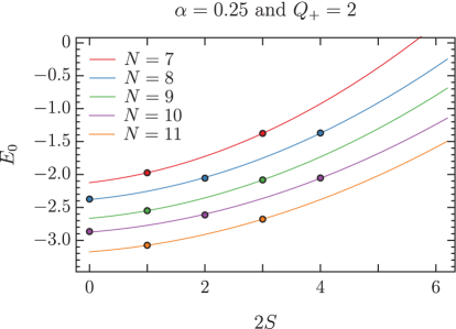
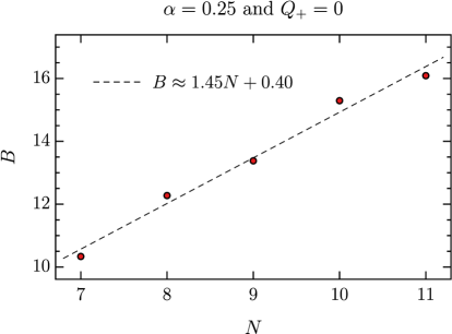
Figure 14: The dependence of ground state energy at $\alpha=0.25$ on $SU(2)$ spin $S$ at $Q_{+}=0,1,2$. We use the Ansatz $E_{0}\approx A+\frac{1}{2B_{+}}Q_{+}^{2}+\frac{2}{B_{\textrm{SU(2)}}}S(S+1)),$ and plot $B_{\textrm{SU(2)}}$ against $N$ to estimate the compressibility, $K_{\textrm{SU(2)}}\approx 1.45.$

Appendix A Particle-hole symmetry

For the single complex SYK model, the Hamiltonian which respects the particle-hole symmetry $c_{i}\leftrightarrow c_{i}^{\dagger}$, accompanied by $J_{ijkl}\rightarrow J^{*}_{ijkl}$, was given in [25]

$$H_{cSYK}=\sum_{i,j,k,l=1}^{N}J_{ijkl}\mathcal{A}\{c_{i}^{\dagger}c_{j}^{\dagger}c_{k}c_{l}\}\ ,$$ (A.1)

where $\mathcal{A}$ denotes total antisymmetrization:

$$\mathcal{A}\{c_{i}^{\dagger}c_{j}^{\dagger}c_{k}c_{l}\}=c_{i}^{\dagger}c_{j}^{\dagger}c_{k}c_{l}+\frac{1}{2}\left(\delta_{ik}c^{\dagger}_{j}c_{l}-\delta_{il}c^{\dagger}_{j}c_{k}+\delta_{jl}c^{\dagger}_{i}c_{k}-\delta_{jk}c^{\dagger}_{i}c_{l}+\frac{1}{2}(\delta_{il}\delta_{jk}-\delta_{ik}\delta_{jl})\right)\ .$$ (A.2)

To make the Hamiltonian of the coupled model, (1.1), invariant under the full particle-hole symmetry (2.5), we have to add to it similar terms:

$$H_{ed}= \sum_{i,j,k,l=1}^{N}J_{ijkl}\bigg{(}\mathcal{A}\{c_{1i}^{\dagger}c_{1j}^{\dagger}c_{1k}c_{1l}\}+\mathcal{A}\{c_{2i}^{\dagger}c_{2j}^{\dagger}c_{2k}c_{2l}\}$$

$$+8\alpha\left(c_{1i}^{\dagger}c_{2j}^{\dagger}c_{2k}c_{1l}-\frac{1}{2}\delta_{jk}c^{\dagger}_{1i}c_{1l}-\frac{1}{2}\delta^{il}c_{2j}^{\dagger}c_{2k}+\frac{1}{4}\delta^{il}\delta_{jk}\right)\bigg{)}\ .$$ (A.3)

This can also be written as

$$H_{ed}= \sum_{i,j,k,l=1}^{N}J_{ijkl}\bigg{(}c_{1i}^{\dagger}c_{1j}^{\dagger}c_{1k}c_{1l}+c_{2i}^{\dagger}c_{2j}^{\dagger}c_{2k}c_{2l}+8\alpha c_{1i}^{\dagger}c_{2j}^{\dagger}c_{2k}c_{1l}$$

$$+(1+2\alpha)\left(-2\delta_{jk}c^{\dagger}_{1i}c_{1l}-2\delta_{il}c_{2j}^{\dagger}c_{2k}+\delta_{il}\delta_{jk}\right)\bigg{)}.$$ (A.4)

The quadratic and c-number terms are subleading in $N$ and thus are not important at large $N.$ They can be important at small $N,$ such as in the exact diagonalizations. We note that these terms vanish for $\alpha=-1/2$, so that the original Hamiltonian (1.1) is automatically particle-hole symmetric for this value of $\alpha$. At another special value, $\alpha=1/4$, the Hamiltonian A.4 respects the $U(2)$ symmetry possessed by the purely quartic Hamiltonian (1.2).

Appendix B Zero modes of the quadratic fluctuations

In this section we give an alternative derivation of the scaling dimension of various primary operators by looking at zero modes of the quadratic fluctuations near the nearly conformal saddle points of the effective action 2.8. We assume the time translational invariance and study fluctuations around the symmetric saddle point. The zero modes of the quadratic fluctuation correspond to the operator three point functions $\delta G_{\sigma\sigma^{\prime}}(\tau)=\langle\frac{1}{N}c^{{\dagger}}_{\sigma i}(\tau)c_{\sigma^{\prime}i}(0)\mathcal{O}_{h}(\infty)\rangle,$ because the DS equations hold up to arbitrary insertion as long as operators are not inserted at $\tau$ or $0.$ In order to not add more contact terms, the operator has to be inserted at $\infty.$ Therefore $\delta G_{\sigma\sigma^{\prime}}(\tau)$ would correspond to a zero mode in the quadratic fluctuation, and the eigenvector dictates the form of the operator. Note in conformal theory, the 3 point functions between primaries are determined up to a constant

$$v(\tau)=\langle\frac{1}{N}c^{{\dagger}}_{\sigma i}(\tau)c_{\sigma^{\prime}i}(0)\mathcal{O}_{h}(\infty)\rangle=\frac{c_{\mathcal{O}}\text{sgn}(\tau)}{|\tau|^{2\Delta-h}},$$ (B.1)

where $h$ is the scaling dimension of the operator $\mathcal{O}$. In order for the three point function to be non-vanishing, the primary operator $\mathcal{O}$ is necessarily bilinear in the elementary fermions, and a $O(N)$ singlet. Therefore one can use this Ansatz to determine the bilinear operator dimension from the quadratic fluctuation. In the following we are going to omit the integrals over $\tau_{1},\tau_{2}$ for brevity.

We are looking for quadratic fluctuations above the conformal saddle point $G_{*12}=G_{*21}=0$ and $G_{*11}=G_{*22}=G_{*}$, where $G_{*}(-\tau)=-G_{*}(\tau)$ and satisfies the Schwinger-Dyson equations

$$\Sigma_{*}(\tau)=J^{2}(1+8\alpha^{2})G_{*}^{3}(\tau),\quad G_{*}(i\omega_{n})(-i\omega_{n}-\Sigma_{*}(i\omega_{n}))=1\,.$$ (B.2)

We find for the second variation

$$\delta^{2}I=\frac{1}{2}G_{*}(\tau_{41})G_{*}(\tau_{23})\textrm{Tr}(\delta\Sigma(\tau_{12})\delta\Sigma(\tau_{34}))-\textrm{Tr}(\delta\Sigma(\tau_{12})\delta G(\tau_{21}))-\frac{J^{2}}{4}\delta^{2}V(G_{ab})\,.$$ (B.3)

It will be convenient to introduce two vectors

$$\delta\textbf{G}(\tau_{12})=(\delta G_{11},\delta G_{22},\delta G_{12},\delta G_{21}),\quad\delta\bm{\Sigma}(\tau_{12})=(\delta\Sigma_{11},\delta\Sigma_{22},\delta\Sigma_{21},\delta\Sigma_{12})$$ (B.4)

then we find

$$\frac{1}{2}G_{*}(\tau_{41})G_{*}(\tau_{23})\textrm{Tr}(\delta\Sigma(\tau_{12})\delta\Sigma(\tau_{34}))=\frac{1}{2}\delta\bm{\Sigma}^{T}(\tau_{12})G_{*}(\tau_{41})G_{*}(\tau_{23})M\delta\bm{\Sigma}(\tau_{34}),$$

$$M=\textrm{diag}(\mathbbm{1},\sigma_{x})$$

$$\delta^{2}V=\delta\textbf{G}^{T}(\tau_{12})G_{*}^{2}(\tau_{12})V\delta\textbf{G}(\tau_{34}),$$

$$V=2\delta(\tau_{13})\delta(\tau_{24})\textrm{diag}(\mathbbm{1}+8\alpha^{2}\sigma_{x},8\alpha^{2}\sigma_{x})-4\delta(\tau_{14})\delta(\tau_{23})\textrm{diag}((1+4\alpha^{2})\mathbbm{1}+4\alpha^{2}\sigma_{x},4\alpha\sigma_{x})$$ (B.5)

where we used that $G_{*}(-\tau)=-G_{*}(\tau)$. Now we can integrate out fluctuations of $\delta\bm{\Sigma}$ fields and find

$$\delta^{2}I=-\frac{1}{2}\delta\textbf{G}^{T}(\tau_{12})\Big{(}\big{(}G_{*}(\tau_{32})G_{*}(\tau_{14})\big{)}^{-1}M+\frac{1}{2}J^{2}G_{*}^{2}(\tau_{12})V\Big{)}\delta\textbf{G}(\tau_{34})\,.$$ (B.6)

Now let us introduce new variables $\textbf{g}(\tau_{12})=|G_{*}(\tau_{12})|S\delta\textbf{G}(\tau_{12})$, where

$$S=\frac{1}{\sqrt{2}}\textrm{diag}(\sigma_{x}-\sigma_{z},\sigma_{x}-\sigma_{z}),\quad S^{T}S=1\,.$$ (B.7)

In terms of the new variables, the variation corresponds to operators $\{O_{2}^{m},O_{1}^{m},O_{4}^{m},O_{3}^{m}\},$ where

$$O_{1,2}^{m}=c_{1i}^{\dagger}\partial_{t}^{m}c_{1i}\pm c_{2i}^{\dagger}\partial_{t}^{m}c_{2i}\ ,\quad O_{3,4}^{m}=c_{1i}^{\dagger}\partial_{t}^{m}c_{2i}\pm c_{2i}^{\dagger}\partial_{t}^{m}c_{1i}\ .$$ (B.8)

We can further decompose g into symmetric $\textbf{g}_{s}(\tau_{12})=\textbf{g}_{s}(\tau_{21})$ and anti-symmetric $\textbf{g}_{a}(\tau_{12})=-\textbf{g}_{a}(\tau_{21})$ sectors under time reflection.

Using the new variables we find

$$\delta^{2}I= \frac{3J^{2}(1+8\alpha^{2})}{2}\textbf{g}_{a}^{T}(\tau_{12})\Big{(}K_{a}^{-1}\textrm{diag}(1,1,-1,1)-\textrm{diag}(\frac{3-8\alpha^{2}}{3(1+8\alpha^{2})},1,-\frac{8\alpha(\alpha+1)}{3\left(1+8\alpha^{2}\right)},\frac{8\alpha(\alpha+1)}{3(1+8\alpha^{2})})\Big{)}\textbf{g}_{a}(\tau_{34})$$

$$-\frac{J^{2}(1+8\alpha^{2})}{2}\textbf{g}_{s}^{T}(\tau_{12})\Big{(}K_{s}^{-1}\textrm{diag}(1,1,-1,1)-\textrm{diag}(1,1,\frac{8\alpha(\alpha-1)}{1+8\alpha^{2}},-\frac{8\alpha(\alpha-1)}{1+8\alpha^{2}})\Big{)}\textbf{g}_{s}(\tau_{34})\,.$$ (B.9)

where $K_{a}$ and $K_{s}$ are standard SYK kernels

$$K_{a}(\tau_{1},\tau_{2};\tau_{3},\tau_{4})=-3J^{2}(1+8\alpha^{2})|G_{*}(\tau_{12})|G_{*}(\tau_{13})G_{*}(\tau_{24})|G_{*}(\tau_{34})|,$$

$$K_{s}(\tau_{1},\tau_{2};\tau_{3},\tau_{4})=-J^{2}(1+8\alpha^{2})|G_{*}(\tau_{12})|G_{*}(\tau_{13})G_{*}(\tau_{24})|G_{*}(\tau_{34})|\,.$$ (B.10)

The scaling dimensions of the bilinear operators $\{O_{1}^{m},O_{2}^{m},O_{3}^{m},O_{4}^{m}\}$ are determined by equating to $1$ the functions (3).

Appendix C Diagrammatic Derivation of the Dyson-Schwinger Equations

The tensor model Hamiltonian (2.11) has four vertices, which we call $v_{1},v_{2},v_{3},v_{4}.$ We write down Dyson-Schwinger equations for all correlators $G_{\sigma\sigma^{\prime}}(\tau,\tau^{\prime})=\frac{1}{N^{3}}\langle\psi^{{\dagger},abc}_{\sigma}(\tau)\psi_{\sigma^{\prime}}^{abc}(\tau^{\prime})\rangle,$ allowed by $SU(N)\times O(N)\times SU(N)$ symmetries. Note $\langle\psi_{1}^{{\dagger},abc}(t)\psi^{{\dagger},abc}_{2}(0)\rangle$ is forbidden by $SU(N)$. This is the tensor counterpart of using the complex $J_{ij,kl}$ in the SYK model.

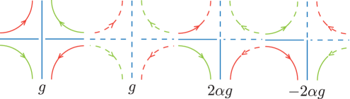
Figure 15: The solid line is for $\psi_{1}$ and dashed $\psi_{2}.$

At large $N$, only the melonic diagrams contribute to the leading order in $N$. The self-energy can be written in terms of Feynman graphs:

Upon drawing the above graphs in the colored line notation, one can check, for example,

$$\Sigma_{11}(\tau) =-g^{2}G_{11}(\tau)^{2}G_{11}(-\tau)-4g^{2}\alpha G_{11}(\tau)G_{12}(\tau)G_{21}(-\tau)-4g^{2}\alpha G_{11}(\tau)G_{21}(\tau)G_{12}(-\tau)$$

$$-2\times(2\alpha g)^{2}G_{11}(\tau)G_{22}(\tau)G_{22}(-\tau)-2\times(2\alpha g)^{2}G_{12}(\tau)G_{21}(\tau)G_{22}(-\tau)\ ,$$ (C.1)

which exactly agrees with $\Sigma_{11}$ in Eq.(4). Similarily $\Sigma_{12}$ agrees. To derive the bilinear spectrum, we shall consider ladder diagrams corrections to 3pt functions along the lines of [1], as an effective action at large $N$ is not available for tensor models.

Appendix D Analytical approximation

If we assume a particular phase such that the $\mathbb{Z}_{4}$ symmetry 2.4 is preserved, the DS equations can be written using one function $G=\left(G_{11}+G_{22}+i\left(G_{12}-G_{21}\right)\right)/2$:

$$(-i\omega-\Sigma(\omega))G(-\omega)=-1\ ,$$

$$\Sigma(\tau)=\tilde{J}^{2}\left(G(\tau)^{3}+kG(\tau)G(-\tau)^{2}\ ,\right)$$ (D.1)

where parameter $k$ is related to $\alpha$ by:

$$k=\frac{3+8\alpha+16\alpha^{2}}{(4\alpha-1)^{2}}\ ,$$ (D.2)

and $\tilde{J}$ is related to $J$ in the standart formulation with $G_{11}$ and $\alpha$ by

$$\tilde{J}^{2}=\frac{J^{2}}{4}(1-4\alpha)^{2}\ .$$ (D.3)

Let us try to use the following ansatz:

$$G(\tau)=\begin{cases}ae^{-\mu\tau}+\dots,&\tau>0\\ -be^{c\mu\tau}+\dots\ ,&\tau<0\ .\end{cases}$$ (D.4)

We have four unknown constants $\mu,c,a,b$, and the dots indicate faster decaying terms. The first DS equation can be rewritten in the time domain as:

$$\partial_{\tau}G(\tau)+\int d\tau^{\prime}\ \Sigma(\tau^{\prime}-\tau)G(\tau^{\prime})=\delta(\tau)\ .$$ (D.5)

Evaluating the convolution for $\tau>0$ yields:

$$A_{1}e^{-\mu\tau}+A_{2+c}e^{-(2+c)\mu\tau}+A_{3c}e^{-3c\mu\tau}$$ (D.6)

The $A_{1},A_{2+c}$ and $A_{3c}$ are easily computed functions of $a,b,c$ and $\mu$:

$$A_{1}=\frac{a^{4}c}{4(c+1)\mu}+\frac{a^{4}}{4(c+1)\mu}-\frac{a^{3}bk}{(c+1)\mu}+\frac{a^{2}b^{2}k}{2(c+1)\mu}+\frac{ab^{3}}{\mu-3c\mu}\ ,$$ (D.7)

$$A_{2+c}=\frac{a^{3}bk}{(c+1)\mu}+\frac{a^{2}b^{2}k}{2(c+1)\mu}\ ,$$ (D.8)

$$A_{3c}=\frac{b^{4}}{4c\mu}-\frac{ab^{3}}{\mu-3c\mu}\ .$$ (D.9)

Terms $e^{-2\mu\tau},e^{-3c\mu\tau}$ are subdominant and were not present in the ansatz, so we can safely ignore them. Therefore we have a single equation:

$$A_{1}=\frac{a\mu}{\tilde{J}}\ .$$ (D.10)

For $\tau<0$ the convolution equals to:

$$B_{c}e^{c\mu\tau}+B_{1+2c}e^{(1+2c)\mu\tau}+B_{3}e^{3\mu\tau}\ ,$$ (D.11)

where

$$B_{c}=\frac{a^{3}b}{(c-3)\mu}+\frac{a^{2}b^{2}k}{2(c+1)\mu}-\frac{ab^{3}k}{(c+1)\mu}+\frac{b^{4}}{4(c+1)\mu}+\frac{b^{4}}{4c(c+1)\mu}\ ,$$ (D.12)

$$B_{1+2c}=\frac{a^{2}b^{2}k}{2(c+1)\mu}+\frac{ab^{3}k}{(c+1)\mu}\ ,$$ (D.13)

$$B_{3}=\frac{a^{4}c}{4(c+1)\mu}+\frac{a^{4}}{4(c+1)\mu}-\frac{a^{3}b}{(c-3)\mu}\ .$$ (D.14)

Let us assume that $c>4$. Then we can again ignore the term $e^{(1+2c)\mu\tau}$. However, the term $e^{3\mu\tau}$ has to be zero. Therefore we have two equations:

$$B_{3}=0\ ,$$ (D.15)

$$B_{c}=\frac{bc\mu}{\tilde{J}}\ .$$ (D.16)

We see that our ansatz is consistent: we managed to eliminate all faster decaying terms. Moreover, we have 4 unknown variables and only three equations. We will empose one extra condition:

$$a+b=1\ .$$ (D.17)

If ansatz (D.4) were an exact solution, then this condition would have followed from having a delta function on the right hand side of DS equations. Unfortunately, (D.4) is not an exact solution and at very small $\tau$ the faster decaying exponential terms become important. However, we still impose eq. (D.17) and demonstrate that it agrees with the numerics. So in the end we have four algebraic equations (D.10), (D.15), (D.16), (D.17) for four unknown variables $a,b,c,\mu$. This system can be easily solved numerically.

For comparison, we solve the DS equations numerically for $\beta\tilde{J}=400$(black dots) and $\beta\tilde{J}=1000$(red dots) and fixing $\tilde{J}=1$. After that, we fit the numerical solution with exponents (D.4). This way we obtain numerical values of $a,b,c,\mu$. The comparison with analytical answer is presented on Figure 16.

Let us note, however, that this approximation does not describe very well the behavior at small Euclidean times $\tau$. Graphs 2 clearly indicate that $G_{12}$ does not have a linear term near $\tau=0$:

$$G_{12}=c_{1}-c_{2}\tau^{2},\ c_{1},c_{2}>0\ .$$ (D.18)

Generically, ansatz (D.4) does have a linear term near $\tau=0$, by the coefficient in front of it is small.

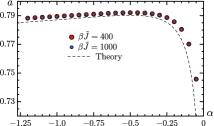
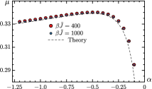
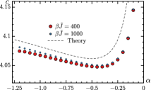
Figure 16: $a,\mu,c$ as a function of $\alpha$. Black dashed line: analytical answer obtained by solving the algebraic system (D.10), (D.15), (D.16), (D.17) numerically. Dots: numerical solution of DS equations. Red dots is $\beta\tilde{J}=400$, blue dots is $\beta\tilde{J}=1000$. In both plots $\tilde{J}=1$.

References

- [1] J. Kim, I. R. Klebanov, G. Tarnopolsky, and W. Zhao, “Symmetry Breaking in Coupled SYK or Tensor Models,” Phys. Rev. X 9 (2019), no. 2 021043, 1902.02287.
- [2] V. Bonzom, R. Gurau, A. Riello, and V. Rivasseau, “Critical behavior of colored tensor models in the large N limit,” Nucl. Phys. B853 (2011) 174–195, 1105.3122.
- [3] A. Kitaev, “A simple model of quantum holography,”. http://online.kitp.ucsb.edu/online/entangled15/kitaev/,http://online.kitp.ucsb.edu/online/entangled15/kitaev2/. Talks at KITP, April 7, 2015 and May 27, 2015.
- [4] A. Kitaev and S. J. Suh, “The soft mode in the Sachdev-Ye-Kitaev model and its gravity dual,” JHEP 05 (2018) 183, 1711.08467.
- [5] E. Witten, “An SYK-Like Model Without Disorder,” J. Phys. A52 (2019), no. 47 474002, 1610.09758.
- [6] I. R. Klebanov and G. Tarnopolsky, “Uncolored random tensors, melon diagrams, and the Sachdev-Ye-Kitaev models,” Phys. Rev. D95 (2017), no. 4 046004, 1611.08915.
- [7] R. Gurau and J. P. Ryan, “Colored Tensor Models - a review,” SIGMA 8 (2012) 020, 1109.4812.
- [8] A. Tanasa, “The Multi-Orientable Random Tensor Model, a Review,” SIGMA 12 (2016) 056, 1512.02087.
- [9] G. Sarosi, “AdS2 holography and the SYK model,” PoS Modave2017 (2018) 001, 1711.08482.
- [10] V. Rosenhaus, “An introduction to the SYK model,” 1807.03334.
- [11] N. Delporte and V. Rivasseau, “The Tensor Track V: Holographic Tensors,” 2018. 1804.11101.
- [12] I. R. Klebanov, F. Popov, and G. Tarnopolsky, “TASI Lectures on Large Tensor Models,” PoS TASI2017 (2018) 004, 1808.09434.
- [13] R. Gurau, “Notes on Tensor Models and Tensor Field Theories,” 1907.03531.
- [14] D. A. Trunin, “Pedagogical introduction to SYK model and 2D Dilaton Gravity,” 2002.12187.
- [15] J. Polchinski and V. Rosenhaus, “The Spectrum in the Sachdev-Ye-Kitaev Model,” JHEP 04 (2016) 001, 1601.06768.
- [16] J. Maldacena and D. Stanford, “Comments on the Sachdev-Ye-Kitaev model,” Phys. Rev. D94 (2016), no. 10 106002, 1604.07818.
- [17] D. J. Gross and V. Rosenhaus, “A Generalization of Sachdev-Ye-Kitaev,” JHEP 02 (2017) 093, 1610.01569.
- [18] A. Jevicki, K. Suzuki, and J. Yoon, “Bi-Local Holography in the SYK Model,” JHEP 07 (2016) 007, 1603.06246.
- [19] Y. Gu, X.-L. Qi, and D. Stanford, “Local criticality, diffusion and chaos in generalized Sachdev-Ye-Kitaev models,” JHEP 05 (2017) 125, 1609.07832.
- [20] J. Maldacena and X.-L. Qi, “Eternal traversable wormhole,” 1804.00491.
- [21] A. M. García-García, T. Nosaka, D. Rosa, and J. J. Verbaarschot, “Quantum chaos transition in a two-site Sachdev-Ye-Kitaev model dual to an eternal traversable wormhole,” Phys. Rev. D 100 (2019), no. 2 026002, 1901.06031.
- [22] S. Sachdev and J. Ye, “Gapless spin fluid ground state in a random, quantum Heisenberg magnet,” Phys. Rev. Lett. 70 (1993) 3339, cond-mat/9212030.
- [23] S. Sachdev, “Bekenstein-Hawking Entropy and Strange Metals,” Phys. Rev. X5 (2015), no. 4 041025, 1506.05111.
- [24] R. A. Davison, W. Fu, A. Georges, Y. Gu, K. Jensen, and S. Sachdev, “Thermoelectric transport in disordered metals without quasiparticles: The Sachdev-Ye-Kitaev models and holography,” Phys. Rev. B95 (2017), no. 15 155131, 1612.00849.
- [25] Y. Gu, A. Kitaev, S. Sachdev, and G. Tarnopolsky, “Notes on the complex Sachdev-Ye-Kitaev model,” JHEP 02 (2020) 157, 1910.14099.
- [26] O. Bohigas and J. Flores, “Two-body random hamiltonian and level density,” Phys. Lett. 34B (1971) 261–263.
- [27] J. B. French and S. S. M. Wong, “Validity of random matrix theories for many-particle systems,” Phys. Lett. 33B (1970) 449–452.
- [28] Y. Alhassid, H. A. Weidenmüller, and A. Wobst, “Disordered mesoscopic systems with interactions: Induced two-body ensembles and the Hartree-Fock approach,” Phys. Rev. B 72 (Jul, 2005) 045318.
- [29] A. A. Patel, M. J. Lawler, and E.-A. Kim, “Coherent superconductivity with large gap ratio from incoherent metals,” Phys. Rev. Lett. 121 (2018), no. 18 187001, 1805.11098.
- [30] Y. Wang, “Solvable Strong-coupling Quantum Dot Model with a Non-Fermi-liquid Pairing Transition,” Phys. Rev. Lett. 124 (2020), no. 1 017002, 1904.07240.
- [31] I. Esterlis and J. Schmalian, “Cooper pairing of incoherent electrons: an electron-phonon version of the Sachdev-Ye-Kitaev model,” Phys. Rev. B100 (2019), no. 11 115132, 1906.04747.
- [32] D. Chowdhury and E. Berg, “Intrinsic superconducting instabilities of a solvable model for an incoherent metal,” arXiv e-prints (Aug, 2019) arXiv:1908.02757, 1908.02757.
- [33] D. Chowdhury and E. Berg, “The unreasonable effectiveness of Eliashberg theory for pairing of non-Fermi liquids,” arXiv e-prints (Dec, 2019) arXiv:1912.07646, 1912.07646.
- [34] D. Hauck, M. J. Klug, I. Esterlis, and J. Schmalian, “Eliashberg equations for an electron–phonon version of the Sachdev–Ye–Kitaev model: Pair breaking in non-Fermi liquid superconductors,” Annals of Physics (Feb, 2020) 168120.
- [35] A. Abanov and A. V. Chubukov, “Interplay between superconductivity and non-Fermi liquid at a quantum-critical point in a metal. I: The -model and its phase diagram at . The case ,” 2020.
- [36] Y. Wang and A. V. Chubukov, “Quantum Phase Transition in the Yukawa-SYK Model,” 2005.07205.
- [37] S. Sahoo, É. Lantagne-Hurtubise, S. Plugge, and M. Franz, “Traversable wormhole and Hawking-Page transition in coupled complex SYK models,” arXiv e-prints (June, 2020) arXiv:2006.06019, 2006.06019.
- [38] A. Kamenev, I. R. Klebanov, A. Milekhin, and G. Tarnopolsky, “unpublished,”.
- [39] D. J. Gross and V. Rosenhaus, “The Bulk Dual of SYK: Cubic Couplings,” JHEP 05 (2017) 092, 1702.08016.
- [40] J. Maldacena, D. Stanford, and Z. Yang, “Conformal symmetry and its breaking in two dimensional Nearly Anti-de-Sitter space,” PTEP 2016 (2016), no. 12 12C104, 1606.01857.
- [41] J. Yoon, “SYK Models and SYK-like Tensor Models with Global Symmetry,” JHEP 10 (2017) 183, 1707.01740.
- [42] J. Liu and Y. Zhou, “Note on global symmetry and SYK model,” JHEP 05 (2019) 099, 1901.05666.
- [43] L. V. Iliesiu, “On 2D gauge theories in Jackiw-Teitelboim gravity,” 1909.05253.
- [44] D. Kapec, R. Mahajan, and D. Stanford, “Matrix ensembles with global symmetries and ’t Hooft anomalies from 2d gauge theory,” JHEP 04 (2020) 186, 1912.12285.