Fairness in Forecasting and Learning Linear Dynamical Systems

Abstract

In machine learning, training data often capture the behaviour of multiple subgroups of some underlying human population. When the amounts of training data for the subgroups are not controlled carefully, under-representation bias arises. We introduce two natural notions of subgroup fairness and instantaneous fairness to address such under-representation bias in time-series forecasting problems. In particular, we consider the subgroup-fair and instant-fair learning of a linear dynamical system (LDS) from multiple trajectories of varying lengths, and the associated forecasting problems. We provide globally convergent methods for the learning problems using hierarchies of convexifications of non-commutative polynomial optimisation problems. Our empirical results on a biased data set motivated by insurance applications and the well-known COMPAS data set demonstrate both the beneficial impact of fairness considerations on statistical performance and encouraging effects of exploiting sparsity on run time.

1 Introduction

The identification of vector autoregressive processes with hidden components from time series of observations is a central problem across Machine Learning, Statistics, and Forecasting (West and Harrison 1997). This problem is also known as proper learning of linear dynamical systems (LDS) in System Identification (Ljung 1998). As a rather general approach to time-series analysis, it has applications ranging from learning population-growth models in actuarial science and mathematical biology to functional analysis in neuroscience. Indeed, one encounters either partially observable processes (Åström 1965) or questions of causality (Pearl 2009) that can be tied to proper learning of LDS (Geiger et al. 2015) in almost any application domain.

A discrete-time model of a linear dynamical system $\mathcal{L}=(G,F,V,W)$ (West and Harrison 1997) suggests that the random variable $Y_{t}\in\mathbb{R}^{m}$ capturing the observed component (output, observations, measurements) evolves over time $t\geq 1$ according to:

$$\phi_{t} = G\phi_{t-1}+w_{t},$$ (1)

$$Y_{t} = F^{\prime}\phi_{t}+v_{t},$$ (2)

where $\phi_{t}\in\mathbb{R}^{n}$ is the hidden component (state) and $G\in\mathbb{R}^{n\times n}$ and $F\in\mathbb{R}^{n\times m}$ are compatible system matrices. Random variables $w_{t},v_{t}$ capture normally-distributed process noise and observation noise, with zero means and covariance matrices $W\in\mathbb{R}^{n\times n}$ and $V\in\mathbb{R}^{m\times m}$, respectively. In this setting, proper learning refers to identifying the quadruple $(G,F,V,W)$ given the observations $\{Y_{t}\}_{t\in\mathbb{N}}$ of $\mathcal{L}$. This also allows for the estimation of subsequent observations, in the so-called “prediction-error” approach to improper learning (Ljung 1998).

We consider a generalisation of the proper learning of LDS, where:

• There are a number of individuals $p\in\mathcal{P}$ within a population. The population $\mathcal{P}$ is partitioned into subgroups indexed by $\mathcal{S}$.

• For each subgroup $s\in\mathcal{S}$, there is a set $\mathcal{I}^{(s)}$ of trajectories of observations available and each trajectory $i\in\mathcal{I}^{(s)}$ has observations for periods $\mathcal{T}^{(i,s)}$, possibly of varying cardinality $|\mathcal{T}^{(i,s)}|$.

• Each subgroup $s\in\mathcal{S}$ is associated with a LDS, $\mathcal{L}^{(s)}$. For all $i\in\mathcal{I}^{(s)}$, $s\in\mathcal{S}$, the trajectory $\{Y_{t}\}^{(i,s)}$, for $t\in\mathcal{T}^{(i,s)}$, is hence generated by precisely one LDS $\mathcal{L}^{(s)}$.

Note that for notations, the superscripts denote the trajectories and subgroups while subscripts indicates the periods. In this setting, under-representation bias (Blum and Stangl 2019, cf. Section 2.2), where the trajectories of observations from one (“disadvantaged”) subgroup are under-represented in the training data, harms both accuracy of the classifier overall and fairness in the sense of varying accuracy across the subgroups. This is particularly important, if the problem is constrained to be subgroup-blind, i.e., constrained to consider only a single LDS as a model. This is the case, when the use of attributes distinguishing each subgroup can be regarded as discriminatory (e.g., gender, race, cf. (Gajane and Pechenizkiy 2017)). Notice that such anti-discrimination measures are increasingly stipulated by the legal systems, e.g., within product or insurance pricing, where the sex of the applicant cannot be used, despite being known.

A natural notion of fairness in subgroup-blind learning of LDS involves estimating the system matrices or forecasting the next output of a single LDS that captures the overall behaviour across all subgroups, while taking into account the varying amounts of training data for the individual subgroups. To formalise this, suppose that we learn one LDS $\mathcal{L}$ from the multiple trajectories and we define a loss function that measures the loss of accuracy for a certain observation $Y_{t}^{(i,s)}$, for $t\in\mathcal{T}^{(i,s)}$, $i\in\mathcal{I}^{(s)}$, $s\in\mathcal{S}$ when adopting the forecast $f_{t}$ for the overall population. For $t\in\mathcal{T}^{(i,s)}$, $i\in\mathcal{I}^{(s)}$, $s\in\mathcal{S}$, we have

$$\operatorname*{loss}^{(i,s)}(f_{t}):=||Y_{t}^{(i,s)}-f_{t}||.$$ (3)

Let $\mathcal{T}^{+}=\cup_{i\in\mathcal{I}^{(s)},s\in\mathcal{S}}\mathcal{T}^{(i,s)}$. We know that $f_{t}$ is feasible only when $t\in\mathcal{T}^{+}$. Note that since each trajectory is of varying length, it is possible that at certain triple $(t,i,s)$, there is no observation and $Y_{t}^{(i,s)}$, $\operatorname*{loss}^{(i,s)}(f_{t})$ become infeasible.

We propose two objective to address the under-representation bias, which extend group fairness (Feldman et al. 2015) to time series:

1. Subgroup Fairness. The objective seeks to equalise, across all subgroups, the sum of losses for the subgroup. Considering the number of trajectories in each subgroup and the number of observations across the trajectories may differ, we include $|\mathcal{I}^{(s)}|,|\mathcal{T}^{(i,s)}|$ as weights:

   $$\min_{f_{t},t\in\mathcal{T}^{+}}\max_{s\in\mathcal{S}}\left\{\frac{1}{|\mathcal{I}^{(s)}|}\sum_{i\in\mathcal{I}^{(s)}}\frac{1}{|\mathcal{T}^{(i,s)}|}\sum_{t\in\mathcal{T}^{(i,s)}}\operatorname*{loss}^{(i,s)}(f_{t})\right\}$$ (4)

2. Instantaneous Fairness. The objective seeks to equalise the instantaneous loss, by minimising the maximum of the losses across all subgroups and all times:

   $$\min_{f_{t},t\in\mathcal{T}^{+}}\left\{\max_{t\in\mathcal{T}^{(i,s)},i\in\mathcal{I}^{(s)},s\in\mathcal{S}}\left\{\operatorname*{loss}^{(i,s)}(f_{t})\right\}\right\}$$ (5)

Following (Zhou and Marecek 2020), we also cast proper and improper learning of a linear dynamical system with such fairness considerations as a non-commutative polynomial optimisation problem (NCPOP), which can be solved efficiently using a globally-convergent hierarchy of semidefinite programming (SDP) relaxations.

Related Work

This presents an algorithmic approach to addressing the under-representation bias studied by (Blum and Stangl 2019) and within the imbalanced learning literature (He and Ma 2013; Brabec et al. 2020, e.g.) and presents a step forward within the fairness in forecasting studied recently by (Gajane and Pechenizkiy 2017; Chouldechova 2017; Locatello et al. 2019), as outlined in the excellent survey of (Chouldechova and Roth 2020). It follows much work on fairness in classification, e.g., (Zliobaite 2015; Hardt, Price, and Srebro 2016; Kilbertus et al. 2017; Kusner et al. 2017; Chouldechova and Roth 2020; Aghaei, Azizi, and Vayanos 2019). It is complemented by several recent studies involving dynamics and fairness (Mouzannar, Ohannessian, and Srebro 2019; Paaßen et al. 2019; Jung et al. 2020), albeit not involving learning of dynamics. It relies crucially on tools developed in non-commutative polynomial optimisation (Pironio, Navascués, and Acín 2010; Wang, Magron, and Lasserre 2019, 2020) and non-commutative algebra (Gelfand and Neumark 1943; Segal 1947; McCullough 2001; Helton 2002), which have not seen much use in Statistics and Machine Learning, yet.

2 Motivation

Insurance Pricing

Let us consider two motivating examples. One important application arises in Actuarial Science. In the European Union, a directive (implementing the principle of equal treatment between men and women in the access to and supply of goods and services), bars insurers from using gender as a factor in justifying differences in individuals’ premiums. In contrast, insurers in many other territories classify insureds by gender, because females and males have different behavior patterns, which affects insurance payments. Take the annuity-benefit scheme for example. It is a well-known fact that females have a longer life expectancy than males (Huang and Salm 2020). The insurer will hence pay more to a female insured over the course of her lifetime, compared to a male insured, on averag (Thiery and Van Schoubroeck 2006). Because of the directive, a unisex mortality table needs to be used. As a result, male insureds receive less benefits, while paying the same premium in total as the female subgroup (Thiery and Van Schoubroeck 2006). Consequently, male insureds might leave the annuity-benefit scheme (known as the adverse selection), which makes the unisex mortality table more challenging to use in the estimation of the life expectancy of the “unisex” population, where female insureds become the advantaged subgroup.

Consider a simple actuarial pricing model of annuity insurance. Insureds enter an annuity-benefit scheme at time $0$ and each insured can receive 1 euro in the end of each year for at most 10 years on the condition that it is still alive. Let $p_{t}$ denotes how many insureds left in the scheme in the end of the $t^{th}$ year. Suppose there are $p_{0}$ insureds in the beginning and the pricing interest rate is $i$ $(i\leq 1)$. The formula of calculating the pure premium is in (6), thus summing up the present values of payment in each year and then divided by the number of insureds in the beginning.

$$\operatorname*{premium}:=\frac{\sum_{t=1}^{10}p_{t}\times(1+i)^{-t}}{p_{0}}$$ (6)

The most important quality $p_{t}$ is derived from estimating insureds’ life expectancy. Suppose the insureds can be divided into female subgroup and male subgroup and each subgroup only have one trajectory: $\{Y_{t}\}^{(\ \cdot\ ,f)}$ for female subgroup, $\{Y_{t}\}^{(\ \cdot\ ,m)}$ for male subgroup for $1\leq t\leq 10$, where the superscript $i$ is dropped. The two trajectories indicate how many female and male insureds are alive in the end of the $t^{th}$ year respectively. Both trajectories can be regarded as linear dynamic systems. We have

$$Y_{t}^{(\ \cdot\ ,f)}= G^{(f)}Y_{t-1}^{(\ \cdot\ ,f)}+\omega_{t}^{(f)}, 2\leq t\leq 10,$$ (7)

$$Y_{t}^{(\ \cdot\ ,m)}= G^{(m)}Y_{t-1}^{(\ \cdot\ ,m)}+\omega_{t}^{(m)}, 2\leq t\leq 10,$$ (8)

$$p_{t}= Y_{t}^{(\ \cdot\ ,f)}+Y_{t}^{(\ \cdot\ ,m)}, 1\leq t\leq 10,$$ (9)

where $\omega_{t}^{(f)}$ and $\omega_{t}^{(m)}$ are measurement noises while $G^{(f)}$ and $G^{(m)}$ are system matrices for female LDS $\mathcal{L}^{(f)}$ and male LDS $\mathcal{L}^{(m)}$ respectively. Note that these are state processes, without any observation process: the number of survivals can be precisely observed. To satisfy the directive, one needs to consider a unisex model:

$$f_{t} = Gf_{t-1}+\omega_{t},\,2\leq t\leq 10,$$ (10)

where $2\leq t\leq 10$ and $\omega_{t}$ and $G$ pertain to the unisex insureds LDS $\mathcal{L}$. Subsequently, the loss functions for female (f) and male (m) subgroups are:

$$\operatorname*{loss}^{(\ \cdot\ ,f)}(f_{t}):= ||Y_{t}^{(\ \cdot\ ,f)}-f_{t}|| ,1\leq t\leq 10,$$ (11)

$$\operatorname*{loss}^{(\ \cdot\ ,m)}(f_{t}):= ||Y_{t}^{(\ \cdot\ ,m)}-f_{t}|| ,1\leq t\leq 10,$$ (12)

Since the trajectories $\{Y_{t}\}^{(\ \cdot\ ,f)}$ and $\{Y_{t}\}^{(\ \cdot\ ,m)}$ have the same length and there is only one trajectory in each subgroup, the two objective (4)-(5) has the form:

$$\min_{f_{t},1\leq t\leq 10}\max\left\{\sum_{t=1}^{10}\operatorname*{loss}^{(\ \cdot\ ,f)}(f_{t}),\sum_{t=1}^{10}\operatorname*{loss}^{(\ \cdot\ ,m)}(f_{t})\right\}$$ (13)

$$\min_{f_{t},1\leq t\leq 10}\left\{\max_{1\leq t\leq 10,s\in\{f,m\}}\left\{\operatorname*{loss}^{(\ \cdot\ ,s)}(f_{t})\right\}\right\}$$ (14)

Personalised Pricing

Another application arises in personalised pricing (PP). For example, Amazon has been found (OECD 2018) to sell certain products to regular consumers at higher prices. This is legal, albeit questionable. In contrast, gender-based price discrimination (Abdou 2019) violates (OECD 2018) anti-discrimination laws in many jurisdictions.

Let us consider an idealised example of PP: Consider a soap retailer, whose customers contain female and male subgroups. Each gender has a specific dynamic system modelling its willing to pay (“demand price” of each subgroup), while the retailer should set a “unisex” price. As in the discussion of insurance pricing, we consider subgroups $S=\{$female, male$\}$ and use superscripts $(f),(m)$ to distinguish the related quantities. Unlike in insurance pricing, the demand price of each customer is regarded as a single trajectory. More importantly, since customers might start buying the soap, quit buying the soap, or move to other substitutes at different time points, those trajectories of demand prices are assumed to be of varying lengths. For example, a customer starts to buy the soap at time $3$ but decides to buy hand wash instead from time $7$.

Let us assume there are $|\mathcal{I}^{(f)}|$ female customers and $|\mathcal{I}^{(m)}|$ customers in the overall time window $\mathcal{T}^{+}$. Let $Y_{t}^{(i,s)}$ denote the estimated demand price at time $t$ of the $i^{th}$ customer in subgroup $s$. These evolve as:

$$\phi_{t}^{f}= G^{(f)}\phi_{t-1}^{(f)}+\omega_{t}^{(f)} ,t\in\mathcal{T}^{+},$$ (15)

$$Y_{t}^{(i,f)}= F^{(f)^{\prime}}\phi_{t}^{(f)}+\nu_{t}^{(i,f)} ,t\in\mathcal{T}^{(i,f)},i\in\mathcal{I}^{(f)},$$ (16)

$$\phi_{t}^{m}= G^{(m)}\phi_{t-1}^{(m)}+\omega_{t}^{(m)} ,t\in\mathcal{T}^{+},$$ (17)

$$Y_{t}^{(i,m)}= F^{(m)^{\prime}}\phi_{t}^{(m)}+\nu_{t}^{(i,m)} ,t\in\mathcal{T}^{(i,m)},i\in\mathcal{I}^{(m)}.$$ (18)

The unisex model for demand price considers the unisex state $m_{t}$, the unisex system matrices $G,F$, and unisex noises $\omega_{t},\nu_{t}$:

$$m_{t}= Gm_{t-1}+\omega_{t} ,\,t\in\mathcal{T}^{+},$$ (19)

$$f_{t}= F^{\prime}m_{t}+\nu_{t} ,\,t\in\mathcal{T}^{+}.$$ (20)

For $\operatorname*{loss}^{(i,f)}(f_{t}):=||Y_{t}^{(i,f)}-f_{t}||,t\in\mathcal{T}^{(i,f)},i\in\mathcal{I}^{(f)}$ and $\operatorname*{loss}^{(i,m)}(f_{t}):=||Y_{t}^{(i,m)}-f_{t}||,t\in\mathcal{T}^{(i,m)},i\in\mathcal{I}^{(m)}$, the two objective (4)-(5) has the form:

$$\min_{f_{t},t\in\mathcal{T}^{+}}\max_{s\in\mathcal{S}}\left\{\frac{1}{|\mathcal{I}^{(s)}|}\sum_{i=1}^{\mathcal{I}^{(s)}}\frac{1}{|\mathcal{T}^{(i,s)}|}\sum_{t\in\mathcal{T}^{(i,s)}}\operatorname*{loss}^{(i,s)}(f_{t})\right\}$$ (21)

$$\min_{f_{t},t\in\mathcal{T}^{+}}\left\{\max_{t\in\mathcal{T}^{(i,s)},i\in\mathcal{I}_{s},s\in\mathcal{S}}\left\{\operatorname*{loss}^{(i,s)}(f_{t})\right\}\right\}$$ (22)

3 Our Models

We assume that the underlying LDS $\mathcal{L}^{(s)}=(G^{(s)},F^{(s)},V^{(s)},W^{(s)})$ of each subgroup $s\in\mathcal{S}$ all have the form of (1)-(2), while only one subgroup-blind LDS $\mathcal{L}$ can be learned and used for prediction. The following model in (23)-(24) can be used to describe the subgroup-blind state evolution directly.

$$m_{t} =Gm_{t-1}+\omega_{t},$$ (23)

$$f_{t} =F^{\prime}m_{t}+\nu_{t}.$$ (24)

for $t\in\mathcal{T}^{+}$, where $m_{t}$ represents the estimated subgroup-blind state and $\{f_{t}\}_{t\in\mathcal{T}^{+}}$ is the trajectory predicted by the subgroup-blind LDS $\mathcal{L}$.

The objectives (4) and (5), subject to (23)-(24), yield two operator-valued optimisation problems. Their inputs are $Y_{t}^{(i,s)},t\in\mathcal{T}^{(i,s)},i\in\mathcal{I}^{(s)},s\in\mathcal{S}$, i.e., the observations of multiple trajectories and the multiplier $\lambda$. The operator-valued decision variables $\mathcal{O}$ include operators proper $F,G$, vectors $m_{t},\omega_{t}$, and scalars $f_{t},\nu_{t},$ and z. Notice that $t$ ranges over $t\in\mathcal{T}^{+}$, except for $m_{t}$, where $t\in\mathcal{T}^{+}\cup\{0\}$. The auxiliary scalar variable $z$ is used to reformulate "$\max$“ in the objective (4) or (5). Since the observation noise is assumed to be a sample of mean-zero normally-distributed random variable, we add the sum of squares of $\nu_{t}$ to the objective with a multiplier $\lambda$, seeking a solution with $\nu_{t}$ close to zero. Overall, the subgroup-fair and instant-fair formulations read:

Oz + λ∑_t≥1 ν_t^2 Subgroup-Fairz≥1|I(s)| ∑_i ∈I^(s) 1|T(i,s)| ∑_t∈T^(i,s) loss^(i,s)(f_t) , s∈S m_t= G m_t-1+ω_t, t∈T^+ f_t= F’ m_t+ν_t, t∈T^+.

Oz + λ∑_t≥1 ν_t^2 Instant-Fairz≥loss^(i,s)(f_t), t∈T^(i,s),i∈I^(s),s∈S m_t= G m_t-1+ω_t, t∈T^+ f_t= F’ m_t+ν_t, t∈T^+.

For comparison, we use a traditional formulation that focuses on minimising the overall loss: O ∑_s ∈S  ∑_i ∈I^(s) ∑_t∈T^(i,s) loss^(i,s)(f_t) + λ∑_t≥1 ν_t^2  Unfairm_t= G m_t-1+ω_t, t∈T^+ f_t= F’ m_t+ν_t, t∈T^+.

To state our main result, we need a technical assumption related to the stability of the LDS, which suggests that the operator-valued decision variables (and hence estimates of states and observations) remain bounded. Let us define the quadratic module, following (Pironio, Navascués, and Acín 2010). Let $Q=\{q_{i}\}$ be the set of polynomials determining the constraints. The positivity domain $\mathbf{S}_{Q}$ of $Q$ are tuples $X=(X_{1},\ldots,X_{n})$ of bounded operators on a Hilbert space $\mathcal{H}$ making all $q_{i}(X)$ positive semidefinite. The quadratic module $M_{Q}$ is the set of $\sum_{i}f_{i}^{{\dagger}}f_{i}+\sum_{i}\sum_{j}g_{ij}^{{\dagger}}q_{i}g_{ij}$ where $f_{i}$ and $g_{ij}$ are polynomials from the same ring. As in (Pironio, Navascués, and Acín 2010), we assume:

Assumption 1 (Archimedean).

Quadratic module $M_{Q}$ of (3) is Archimedean, i.e., there exists a real constant $C$ such that $C^{2}-(X_{1}^{{\dagger}}X_{1}+\cdots+X_{2n}^{{\dagger}}X_{2n})\in M_{Q}$.

Our main result shows that it is possible to recover the quadruple $(G,F,V,W)$ of the subgroup-blind $\mathcal{L}$ with guarantees of global convergence:

Theorem 2.

For any observable linear system $\mathcal{L}=(G,F,V,W)$, for any length $\mathcal{T}^{+}$ of a time window, and any error $\epsilon>0$, under Assumption 1, there is a convex optimisation problem from whose solution one can extract the best possible estimate of system matrices of a system $\mathcal{L}$ based on the observations, with fairness subgroup-fair considerations (3), up to an error of at most $\epsilon$ in Frobenius norm. Furthermore, with suitably modified assumptions, the result holds also for the instant-fair considerations (3).

The proof is available in the full version of the paper on-line (Zhou, Marecek, and Shorten 2020). It relies on the work of (Pironio, Navascués, and Acín 2010), which shows the existence of a sequence of convex optimisation problems, whose objective function approaches the optimum of the non-commutative polynomial optimisation problem, and on the work of Gelfand, Naimark, and Segal (Gelfand and Neumark 1943; Segal 1947; Klep, Povh, and Volcic 2018), which makes it possible to extract the minimiser of the non-commutative polynomial optimisation problem from the solution of the convex optimisation problem.

4 Numerical Illustrations

Generation of Biased Training Data

To illustrate the impact of our models on data with varying degrees of under-representation bias, we consider a method for generating data resembling the motivating applications in Section 2, with varying degrees of the bias. Suppose there is one advantaged subgroup and one disadvantaged subgroup, $S=\{$advantaged, disadvantaged$\}$ with trajectories $\mathcal{I}^{(a)}$ and $\mathcal{I}^{(d)}$ in each subgroup. Under-representation bias can enter training set in the following steps:

1. Observations $Y^{(i,s)}_{t}$ are sampled from corresponding LDS $\mathcal{L}^{(s)}$. Thus each $Y^{(i,s)}_{t}\sim\mathcal{L}^{(s)}$.

2. Discard some trajectories in $\mathcal{I}^{(d)}$, if necessary, such that $|\mathcal{I}^{(a)}|\geq|\mathcal{I}^{(d)}|$.

3. Let $\mathcal{\beta}^{(s)},s\in\mathcal{S}$ denote the probability that an observation from subgroup $s$ stays in the training data and $0\leq\beta^{(s)}\leq 1$. Discard more observations of $\mathcal{I}^{(d)}$ than those of $\mathcal{I}^{(a)}$ so that $\mathcal{\beta}^{(a)}\geq\mathcal{\beta}^{(d)}$. If $\mathcal{\beta}^{(a)}$ is fixed at 1, the degree of under-representation bias can be controlled by simply adjusting $\mathcal{\beta}^{(d)}$.

The last two steps discard more observations of the disadvantaged subgroup in the biased training data, so that the advantaged subgroup becomes over-represented. Note that for small sample size, it is necessary to make sure there is at least one observation in each subgroup at each period.

Consider that both subgroups $\mathcal{L}^{(s)},s\in\mathcal{S}$ have the same system matrices:

$$G^{(s)}=\begin{bmatrix}0.99&0\\ 1.0&0.2\end{bmatrix},F^{(s)}=\begin{bmatrix}1.1\\ 0.8\end{bmatrix},$$

while the covariance matrices $V^{(s)},W^{(s)},s\in\mathcal{S}$ are sampled randomly from a uniform distribution over $[0,1)$ and $[0,0.1)$, respectively. The initial states $m_{0}^{(s)}$ of each subgroups are $5$ and $7$. We set the time window to be $20$ across $3$ trajectories in the advantaged subgroup and $2$ in disadvantaged one, i.e., $|\mathcal{T}^{+}|=20$, $|\mathcal{I}^{(a)}|=3$ and $|\mathcal{I}^{(d)}|=2$. Then the bias is introduced according to the biased training data generalisation process described above, with random $\beta^{(s)},s\in\mathcal{S}$.

Figure 2 shows the forecasts in 30 experiments on this example. For each experiment, the same set of observations $Y_{t}^{(i,s)},t\in\mathcal{T}^{(i,s)}$, $i\in\mathcal{I}^{(s)}$, $s\in\mathcal{S}$ is reused and the trajectories of advantaged and disadvantaged subgroups are denoted by dotted lines and dashed lines, respectively. However, the observations that are discarded vary across the experiments. Thus, a new biased training set is generated in each experiment, albeit based on the same “ground set” of observations. The three models (3)-(3) are applied in each experiment with $\lambda$ of 5 and 1, respectively, as chosen by iterating over integers 1 to 10. The mean of forecast $f$ and its standard deviation are displayed as the solid curves with error bands.

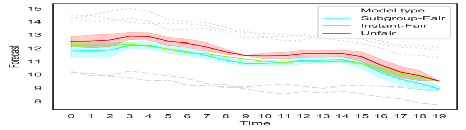
Figure 1: Forecast obtained using (3)-(3): the solid lines in primary colours with error bands display the mean and standard deviation of the forecasts over 10 experiments. For reference, dotted lines and dashed lines in grey denote the trajectories of observations of advantaged and disadvantaged subgroups, respectively, before discarding any observations.

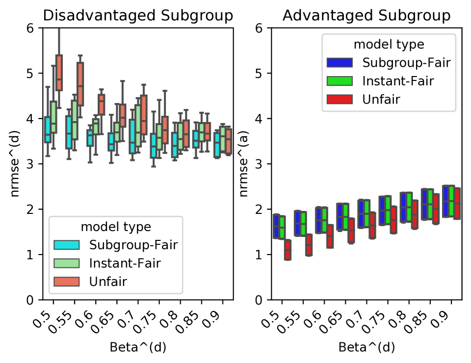
Figure 2: Accuracy as a function of the degree of under-representation bias: The boxplot of $\operatorname*{nrmse}^{(s)},s\in\mathcal{S}$ against $\mathcal{\beta}^{(d)}$, where $\mathcal{\beta}^{(d)}=[0.5,0.55,\dots,0.9]$, with boxes for the quartiles of $\operatorname*{nrmse}^{(s)}$ obtained from $5$ experiments, using the observations in Figure 2.

Effects of Under-Representation Bias on Accuracy

Figure 2 suggests how the degree of bias affects accuracy with and without considering fairness. With the number of trajectories in both subgroups set to 2, i.e. $|I_{a}|=|I_{d}|=2$ and $\mathcal{\beta}^{(a)}=1$, we vary the degree of bias $\mathcal{\beta}^{(d)}$ within $0.5\leq\mathcal{\beta}^{(d)}\leq 1$. To measure the effect of the degree on accuracy, we introduce the normalised root mean squared error (nrmse) fitness value for each subgroup $s\in\mathcal{S}$:

$$\mathrm{\operatorname*{nrmse}^{(s)}}:=\sqrt{\frac{\sum_{i\in\mathcal{I}^{(s)}}\sum_{t\in\mathcal{T}^{(i,s)}}\left(Y_{t}^{(i,s)}-f_{t}\right)^{2}}{\sum_{i\in\mathcal{I}^{(s)}}\sum_{t\in\mathcal{T}^{(i,s)}}\left(Y_{t}^{(i,s)}-\operatorname*{mean}^{(s)}\right)^{2}}},$$ (25)

where $\operatorname*{mean}^{(s)}:=\frac{1}{|\mathcal{I}^{(s)}|}\sum_{i\in\mathcal{I}^{(s)}}\frac{1}{|\mathcal{T}^{(i,s)}|}\sum_{t\in\mathcal{T}^{(i,s)}}Y_{t}^{(i,s)}$. Higher $\operatorname*{nrmse}^{(s)}$ indicates lower accuracy for subgroup $s$, i.e., the predicted trajectory of subgroup-blind $\mathcal{L}$ is further away from the subgroup.

For the training data, the same set of observations $Y_{t}^{(i,s)},t\in\mathcal{T}^{(i,s)}$, $i\in\mathcal{I}^{(s)}$, $s\in\mathcal{S}$ in Figure 2 is reused but $|I_{a}|=|I_{d}|=2$. Thus one trajectory in advantaged subgroup is discarded. Then, the biased training data generalisation process in Section 4 is applied in each experiment with $\mathcal{\beta}^{(a)}=1$ and the values for $\mathcal{\beta}^{(d)}$ selecting from $0.5$ to $0.9$ at the step of $0.05$. At each value of $\mathcal{\beta}^{(d)}$, three models (3)-(3) are run with new biased training data and the experiment is repeated for $5$ times. Hence, the quartiles of $\operatorname*{nrmse}^{(s)}$ for each subgroup shown as boxes in Figure 2.

One could expect that nrmse fitness values of advantaged subgroup in Figure 2 to be generally lower than those of the disadvantaged subgroup ($\operatorname*{nrmse}^{(d)}\geq\operatorname*{nrmse}^{(a)}$), leaving a gap. Those gaps narrow down as $\mathcal{\beta}^{(d)}$ increases, simply because more observations of disadvantaged subgroup remain in the training data. Compared the to “Unfair”, models with fairness constraints, i.e., “Subgroup-Fair” and “Instant-Fair”, show narrower gaps and higher fairness between two subgroups. More surprisingly, when $\operatorname*{nrmse}^{(a)}$ decreases as $\mathcal{\beta}^{(d)}$ gets close to $0.5$, "Subgroup-Fair" model still can keep the $\operatorname*{nrmse}^{(d)}$ at almost the same level, indicating a rise in overall accuracy. This is in contrast with results (Zliobaite 2015; Dutta et al. 2020) from classification.

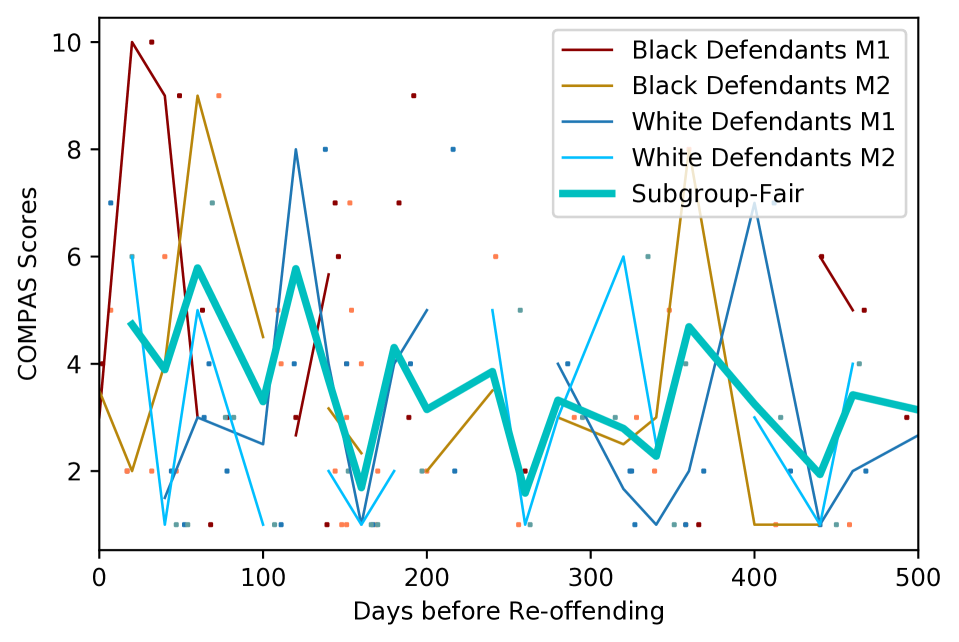
Figure 3: COMPAS recidivism scores of black and white defendants against the actual days before their re-offending. The sample of defendants’ scores are divided into $4$ sub-samples based on race and type of re-offending, distinguished by colours. Dots and curves with the same colour denote the scores of one sub-sample and the trajectory extracted from the scores respectively. The cyan curve displays the result of "Subgroup-Fair" model with $4$ trajectories.

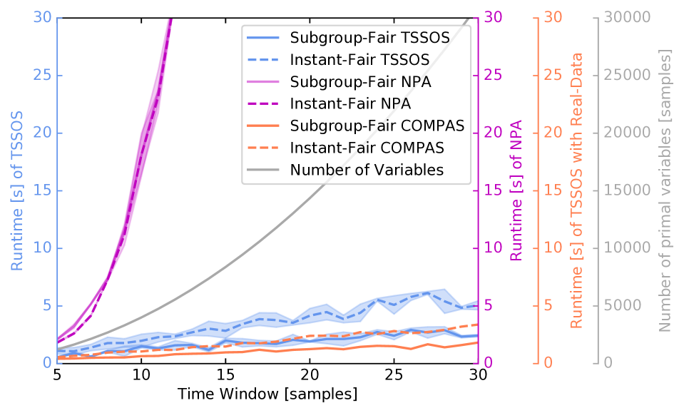
Figure 4: The dimensions of relaxations and the run-time of SDPA thereupon as a function of the length of time window. Run-time of TSSOS and NPA is displayed in cornflower-blue and deep-pink curves, respectively, while the grey curve shows the number of variables in relaxations. Additionally, the run-time of the COMPAS dataset of Figure 4 using TSSOS is also displayed as coral-coloured curves. For run-time, the mean and mean $\pm$ 1 standard deviations across $3$ runs are presented by curves with shaded error bands.

Run-Time

Notice that minimising multivariate operator-valued polynomial optimization problems (3)-(3) is non-trivial, but that there exists sparsity-exploiting variants (TSSOS) of the globally convergent Navascués-Pironio-Acín (NPA) hierarchy used in the proof of Theorem 2. See (Klep, Magron, and Povh 2019; Wang, Magron, and Lasserre 2019, 2020; Wang and Magron 2020). The SDP of a given order in the respective hierarchy can be constructed using ncpol2sdpa of (Wittek 2015) or the tools of (Wang and Magron 2020) and solved by sdpa of (Yamashita, Fujisawa, and Kojima 2003). Our implementation is available on-line at https://github.com/Quan-Zhou/Fairness-in-Learning-of-LDS.

In Figure 4, we illustrate the run-time and size of the relaxations as a function of the length of the time window with the same data set as above (i.e., Figure 2). The grey curve displays the number of variables in the first-order SDP relaxation of "Subgroup-Fair" and "Instant-Fair" models against the length of time window. The deep-pink and cornflower-blue curves show the run-time of the first-order SDP relaxation of NPA and the second-order SDP relaxation of TSSOS hierarchy, respectively, on a laptop equipped by Intel Core i7 8550U at 1.80 Ghz. The results of "Subgroup-Fair" and "Instant-Fair" models are presented by solid and dashed curves, respectively. Since each experiment is repeated for three times, the mean and mean $\pm$ 1 standard deviation of run-time are presented by curves with shaded error bands. It is clear that the run-time of TSSOS exhibits a modest growth with the length of time window, while that of the plain-vanilla NPA hierarchy grows much faster.

An Alternative Approach to COMPASS Dataset

Finally, we wish to suggest the broader applicability of the two notions of subgroup fairness and instantaneous fairness. We use the well-known dataset (Angwin et al. 2016) of estimates of the likelihood of recidivism made by the Correctional Offender Management Profiling for Alternative Sanctions (COMPAS), as used by courts in the United States. The dataset comprises of defendants’ gender, race, age, charge degree, COMPAS recidivism scores, two-year recidivism label, as well as information on prior incidents. The two-year recidivism label denotes whether a person got rearrested within two years (label 1) or not (label 0). If the two-year recidivism label is $1$, there is also information of the recharge degree and the number of days until the person got rearrested. We choose $119$ defendants with recidivism label 1, who are African-American or Caucasian, male, within the age range of 25-45, and with prior crime counts less than 2, with charge degree M and recharge degree M1 or M2. The defendants are partitioned into two subgroups by their ethnicity and then partitioned by the type of their recharge degree (M1 or M2). Hence, we obtain the $4$ sub-samples.

In the days-to-reoffend-vs-score plot, such as Figure 4, dots suggest COMPAS recidivism scores of the $4$ sub-samples against the days before rearrest. Curves capture models, either subgroup-dependent (plotted thin) or Subgroup-Fair (plotted thick). The thick cyan curve is the race-blind prediction from our Subgroup-Fair method, which equalizes scores across the two subgroups. Ideally, one should like to see a smooth, monotonically decreasing curves, overlapping across all subgroup-dependent models. For each sub-sample, aggregate deviation from the Subgroup-Fair curve would be similar to the aggregate deviations of other sub-samples.

In the actual fact, dots are far removed from the ideal monotonically decreasing curve. Also, the subgroup-specific curves (plotted thin) are very different from each other (“subgroup-specific models are unfair”). Specifically, the red and yellow curves are above the sky blue and cornflower blue curves (“at the same risk level, white defendants get lower COMPAS scores”). Notice that the subgroup-dependent models are obtained as follows: we discretise time to $20$-day periods. For each subgroup, we check if anyone re-offends within $20$ days (the first period). If so, the (average) COMPAS score (for all cases within the 20 days) is recorded as the observation of first period of the trajectory of the sub-sample. If not, there is no observation of this period. We repeat this for the subsequent periods and for the three other sub-samples.

In Figure 4, the coral-coloured curve (for the COMPAS dataset) suggests that the run-time remains modest, even as the length of the time window grows to 30.

5 Conclusions

Overall, the two natural notions of fairness (subgroup fairness and instantaneous fairness), which we have introduced, may help establish the study of fairness in forecasting and learning of linear dynamical systems. We have presented globally convergent methods for the estimation considering the two notions of fairness using hierarchies of convexifications of non-commutative polynomial optimisation problems. The run-time of standard solvers for the convexifications is independent of the dimension of the hidden state.

An interesting direction for further research extends the two notions of fairness towards distributional robustness (Hashimoto et al. 2018) and uses the notions of fairness in constraints (Donini et al. 2018), as well as in the objective.

6 Background

In this paper, we consider the case of multiple variants of the LDS and conduct proper learning of the LDS in a way of fairness using the technologies of non-commutative polynomial optimisation. In Section 6, we firstly set our work in the context of system identification and control theory. Secondly, we introduce the concept of fairness, which can be used to deal with multiple variants of the LDS. In the end of this section, we provide a brief overview of non-commutative polynomial optimisation, pioneered by (Pironio, Navascués, and Acín 2010) and nicely surveyed by (Burgdorf, Klep, and Povh 2016), which is our key technical tool.

Related work in system identification and control

Research within System Identification variously appears in venues associated with Control Theory, Statistics, and Machine learning. We refer to (Ljung 1998) and (Tangirala 2014) for excellent overviews of the long history of research in the field, going back at least to (Åström and Torsten 1965). In this section, we focus on pointers to key more recent publications. In improper learning of LDS, a considerable progress has been made in the analysis of predictions for the expectation of the next measurement using auto-regressive (AR) processes. In (Anava et al. 2013), first guarantees were presented for auto-regressive moving-average (ARMA) processes. In (Liu et al. 2016), these results were extended to a subset of autoregressive integrated moving average (ARIMA) processes. (Kozdoba et al. 2019) have shown that up to an arbitrarily small error given in advance, AR($s$) will perform as well as any Kalman filter on any bounded sequence. This has been extended by (Tsiamis and Pappas 2020) to Kalman filtering with logarithmic regret. Another stream of work within improper learning focuses on sub-space methods (Katayama 2006; Van Overschee and De Moor 1996) and spectral methods. (Tsiamis, Matni, and Pappas 2019; Tsiamis and Pappas 2019) presented the present-best guarantees for traditional sub-space methods. Within spectral methods, (Hazan, Singh, and Zhang 2017) and (Hazan et al. 2018) have considered learning LDS with input, employing certain eigenvalue-decay estimates of Hankel matrices in the analyses of an auto-regressive process in a dimension increasing over time. We stress that none of these approaches to improper learning are “prediction-error”: They do not estimate the system matrices.

In proper learning of LDS, many state-of-the-art approaches consider the least-squares method, despite complications encountered in unstable systems (Faradonbeh, Tewari, and Michailidis 2018). (Simchowitz et al. 2018) have provided non-trivial guarantees for the ordinary least-squares (OLS) estimator in the case of stable $G$ and there being no hidden component, i.e., $F^{\prime}$ being an identity and $Y_{t}=\phi_{t}$. Surprisingly, they have also shown that more unstable linear systems are easier to estimate than less unstable ones, in some sense. (Simchowitz, Boczar, and Recht 2019) extended the results to allow for a certain pre-filtering procedure. (Sarkar and Rakhlin 2019) extended the results to cover stable, marginally stable, and explosive regimes.

Our work could be seen as a continuation of the least squares method to processes with hidden components, with guarantees of global convergence. In Computer Science, our work could be seen as an approximation scheme (Vazirani 2013), as it allows for $\epsilon$ error for any $\epsilon>0$.

Fairness in machine learning

The last two years have seen an unprecedented explosion in attention of fairness in the field of artificial intelligence and machine learning (Chouldechova and Roth 2020).

In machine learning, the training set might have biased representations of its subgroups, even when sampled with equal weight (Samadi et al. 2018). Hence, a predictor trained from biased data set and aimed at maximising the overall accuracy might cause different distribution of errors in different subgroups, therefore not correspond to a fair decision-making procedure. High accuracy need not be the primary goal of the system, especially when we consider that “accuracy” is measured on unfair data (Foulds et al. 2020). In facial recognition, (Buolamwini and Gebru 2018) find out that darker-skinned females are the most misclassified subgroup with error rates of up to 34.7% while the maximum error rate for lighter-skinned males is 0.8% as a result of the imbalanced gender and skin type distribution of the datasets of facial analysis benchmarks. Another threat facing us is gender bias shown in word embedding where the word female is tender to be associated to receptionist (Bolukbasi et al. 2016).

According to the clear summary in (Chouldechova and Roth 2020), the definition of fairness can be derived from a statistical notion and an individual notion. The statistical definition of fairness is to request a classifier’s statistic, such as raw positive classification rate (also sometimes known as statistical parity), false positive and false negative rates (also sometimes known as equalised odds), be equalised across the subgroups so that the error caused by the algorithm be proportionately spread across subgroups (Chouldechova and Roth 2020). The statistical definition has a natural connection with Principal Component Analysis (PCA). Introduced in (Samadi et al. 2018), the Fair-PCA problem aims to minimise the maximum construction loss of different subgroups when looking for a lower dimensional representation. To solve the Fair-PCA problem, (Sharifi-Malvajerdi, Kearns, and Roth 2019) design an oracle-efficient algorithm while (Tantipongpipat et al. 2019) propose an algorithms based on extreme-point solutions of semi-definite programs.

The individual definition asks for constraints that bind on specific pairs of individuals, rather than on a quantity that is averaged over groups (Chouldechova and Roth 2020), or in other words, it requires “similar individuals should be treated similarly” (Dwork et al. 2012). This definition is discussed less on account of its requirement of making significant assumptions even through it has strong individual level semantics that one’s risk of being harmed by the error of the classifier are no higher than they are for anyone else (Sharifi-Malvajerdi, Kearns, and Roth 2019).

We can introduce fairness to learning of LDS when dealing with multiple variants of the LDS. When estimating the next observation, one might be given several trajectories of observations from unknown variants of the LDS. In this case, fairness asks to find a suitable model that treats each LDS equally.

Learning from Imbalanced data

Traditional machines learning algorithms can be biased towards majority class over-prevalence (Chawla 2003), i.e., the under-representation bias (Blum and Stangl 2019). Also, the cost of misclassifying an abnormal event (minority class) as a normal event (majority class) is often relatively high (Chawla et al. 2008, 2002). For example, in the case of fraud, diseases, those cases are rare but able to cause serious damages, so it is of great interest to research. The benchmark of learning from imbalanced data was pioneered by (Chawla et al. 2002). They proposed the Synthetic Minority Over-sampling Technique (SMOTE), such that a combination of over-sampling the minority class and under-sampling the majority class can efficiently improve the classifier performance.

The research in learning from imbalanced data has been extensively studied with a particular focus on classification and other predictive contexts as many real-world applications are already facing this problem (Torgo et al. 2017; Fernández et al. 2018). SMOTE has been successfully extended to a variety of applications because of its simplicity and robustness (Cieslak and Chawla 2008). Surprisingly, (Chawla et al. 2008) provides an algorithm that automatically discovers the amount of re-sampling. One the other hand, (Moniz, Branco, and Torgo 2017) proposed the concept of temporal and relevance bias in extension of re-sampling strategies. For the clear journey of SMOTE, please refer to (Fernández et al. 2018).

Unlike the common solution of re-sampling, we address the under-representation bias from the view of optimisation, such that the “loss”, or other statistical performance is equalised over majority and minority subgroups.

Non-commutative polynomial optimisation

In learning of the LDS, the key technical tool of this paper is non-commutative polynomial optimisation (NCPOP), first introduced by (Pironio, Navascués, and Acín 2010). Here, we provide a brief summary of their results, and refer to (Burgdorf, Klep, and Povh 2016) for a book-length introduction. NCPOP is an operator-valued optimisation problem with a standard form in Problem 6:

(H,X,ϕ) ⟨ϕ,p(X)ϕ⟩P:p*= q_i(X)≽0, i=1,…,m ⟨ϕ,ϕ⟩= 1,

where $X=(X_{1},\ldots,X_{n})$ is a bounded operator on a Hilbert space $\mathcal{H}$. The normalised vector $\phi$, i.e., $\|\phi\|^{2}=1$ is also defined on $\mathcal{H}$ with inner product $\langle\phi,\phi\rangle$ equals to $1$. $p(X)$ and $q_{i}(X)$ are polynomials and $q_{i}(X)\succcurlyeq 0$ denotes that the operator $q_{i}(X)$ is positive semi-definite. Polynomials $p(X)$ and $q_{i}(X)$ of degrees $\deg(p)$ and $\deg(q_{i})$, respectively, can be written as:

$$p(X)=\sum_{|\omega|\leq\deg(p)}p_{\omega}\omega,\quad q_{i}(X)=\sum_{|\mu|\leq\deg(q_{i})}q_{i,\mu}\mu,$$ (26)

where $i=1,\ldots,m$. Following (Akhiezer and Krein 1962), we can define the moments on field $\mathbb{R}$ or $\mathbb{C}$, with a feasible solution $(H,X,\phi)$ of problem (6):

$$y_{\omega}=\langle\phi,\omega(X)\phi\rangle,$$ (27)

for all $\omega\in\mathcal{W}_{\infty}$ and $y_{1}=\langle\phi,\phi\rangle=1$. Given a degree $k$, the moments whose degrees are less or equal to $k$ form a sequence of $y=(y_{\omega})_{|\omega|\leq 2k}$. With a finite set of moments $y$ of degree $k$, we can define a corresponding $k^{th}$ order moment matrix $M_{k}(y)$:

$$M_{k}(y)(\nu,\omega)=y_{\nu^{{\dagger}}\omega}=\langle\phi,\nu^{{\dagger}}(X)\omega(X)\phi\rangle,$$ (28)

for any $|\nu|,|\omega|\leq k$ and a localising matrix $M_{k-d_{i}}(q_{i}y)$:

$$M_{k-d_{i}}(q_{i}y)(\nu,\omega) =\sum_{|\mu|\leq\deg(q_{i})}q_{i,\mu}y_{\nu^{{\dagger}}\mu\omega}$$ (29)

$$=\sum_{|\mu|\leq\deg(q_{i})}q_{i,\mu}\langle\phi,\nu^{{\dagger}}(X)\mu(X)\omega(X)\phi\rangle,$$

for any $|\nu|,|\omega|\leq k-d_{i}$, where $d_{i}=\lceil\deg(q_{i})/2\rceil$. The upper bounds of $|\nu|$ and $|\omega|$ are lower than the that of moment matrix because $y_{\nu^{{\dagger}}\mu\omega}$ is only defined on $\nu^{{\dagger}}\mu\omega\in\mathcal{W}_{2k}$ while $\mu\in\mathcal{W}_{\deg(q_{i})}$.

If $(H,X,\phi)$ is feasible, one can utilize the Sums of Squares theorem of (Helton 2002) and (McCullough 2001) to derive semidefinite programming (SDP) relaxations. In particular, we can obtain a $k^{th}$ order SDP relaxation of the non-commutative polynomial optimization problem (6) by choosing a degree $k$ that satisfies the condition of $2k\geq\max\{\deg(p),\max_{i}\deg(q_{i})\}$. The SDP relaxation of order $k$, which we denote $R_{k}$, has the form:

y=(y_ω)_|ω|≤2k ∑_|ω|≤d p_ω y_ωR_k:p^k= M_k(X)≽0 M_k-d_i(q_i X)≽0, i=1,…,m ⟨ϕ,ϕ⟩= 1,

Let us define the quadratic module, following (Pironio, Navascués, and Acín 2010). Let $Q=\{q_{i}\}$ be the set of polynomials determining the constraints. The positivity domain $\mathbf{S}_{Q}$ of $Q$ are tuples $X=(X_{1},\ldots,X_{n})$ of bounded operators on a Hilbert space $\mathcal{H}$ making all $q_{i}(X)$ positive semidefinite. The quadratic module $M_{Q}$ is the set of $\sum_{i}f_{i}^{{\dagger}}f_{i}+\sum_{i}\sum_{j}g_{ij}^{{\dagger}}q_{i}g_{ij}$ where $f_{i}$ and $g_{ij}$ are polynomials from the same ring. As in (Pironio, Navascués, and Acín 2010), we assume:

Assumption 3 (Archimedean).

Quadratic module $M_{Q}$ of (6) is Archimedean, i.e., there exists a real constant $C$ such that $C^{2}-(X_{1}^{{\dagger}}X_{1}+\cdots+X_{2n}^{{\dagger}}X_{2n})\in M_{Q}$, where $X_{n+i},i\in\{1,\dots,n\}$ are defined to be $X_{i}^{{\dagger}}$.

If the Archimedean assumption is satisfied, (Pironio, Navascués, and Acín 2010) have shown that $\lim_{k\to\infty}p^{k}=p^{*}$ for a finite $k$.

Proof of Theorem 2

First, we need to show the existence of a sequence of convex optimisation problems, whose objective function approaches the optimum of the non-commutative polynomial optimisation problem. As explained in the subsection above, (Pironio, Navascués, and Acín 2010) shows that, indeed, there are natural semidefinite programming problems, which satisfy this property. In particular, the existence and convergence of the sequence is shown by Theorem 1 of (Pironio, Navascués, and Acín 2010), which requires Assumption 1.

Notice that we can use the so-called rank-loop condition of (Pironio, Navascués, and Acín 2010) to detect global optimality. Once optimality is detected, it is possible to extract the global optimum $(H^{*},X^{*},\phi^{*})$ from the optimal solution $y$ of problem $R_{k}$, by Gram decomposition; cf. Theorem 2 in (Pironio, Navascués, and Acín 2010). Simpler procedures for the extraction have been considered, cf. (Henrion and Lasserre 2005), but remain less well understood.

More broadly, we would like to show the extraction of the minimiser from the SDP relaxation of order $k(\epsilon)$ in the series is possible. There, one utilises the Gelfand–Naimark–Segal (GNS) construction (Gelfand and Neumark 1943; Segal 1947), as explained in Section 2.2 of (Klep, Povh, and Volcic 2018), which does not require the rank-loop condition to be satisfied, We refer to Section 2.2 of (Klep, Povh, and Volcic 2018) and Section 2.6 of (Dixmier 1969) for details.

References

- Åström (1965) Åström, K. J. 1965. Optimal control of Markov processes with incomplete state information. Journal of Mathematical Analysis and Applications 10(1): 174 – 205. ISSN 0022-247X.
- Åström and Torsten (1965) Åström, K.-J.; and Torsten, B. 1965. Numerical Identification of Linear Dynamic Systems from Normal Operating Records. IFAC Proceedings Volumes 2(2): 96–111. ISSN 1474-6670. 2nd IFAC Symposium on the Theory of Self-Adaptive Control Systems, Teddington, UK, September 14-17, 1965.
- Abdou (2019) Abdou, D. S. 2019. Gender-Based Price Discrimination: The Cost of Being a Woman. Proceedings of Business and Economic Studies 2(5).
- Aghaei, Azizi, and Vayanos (2019) Aghaei, S.; Azizi, M. J.; and Vayanos, P. 2019. Learning optimal and fair decision trees for non-discriminative decision-making. In Proceedings of the AAAI Conference on Artificial Intelligence, volume 33, 1418–1426.
- Akhiezer and Krein (1962) Akhiezer, N. I.; and Krein, M. 1962. Some questions in the theory of moments, volume 2. American Mathematical Society.
- Anava et al. (2013) Anava, O.; Hazan, E.; Mannor, S.; and Shamir, O. 2013. Online Learning for Time Series Prediction. In COLT 2013 - The 26th Annual Conference on Learning Theory, June 12-14, 2013, Princeton University, NJ, USA.
- Angwin et al. (2016) Angwin, J.; Larson, J.; Mattu, S.; and Kirchner, L. 2016. Machine bias. ProPublica, May 23: 2016.
- Blum and Stangl (2019) Blum, A.; and Stangl, K. 2019. Recovering from Biased Data: Can Fairness Constraints Improve Accuracy? arXiv preprint arXiv:1912.01094 .
- Bolukbasi et al. (2016) Bolukbasi, T.; Chang, K.-W.; Zou, J. Y.; Saligrama, V.; and Kalai, A. T. 2016. Man is to computer programmer as woman is to homemaker? debiasing word embeddings. In Advances in neural information processing systems, 4349–4357.
- Brabec et al. (2020) Brabec, J.; Komárek, T.; Franc, V.; and Machlica, L. 2020. On Model Evaluation Under Non-constant Class Imbalance. In Computational Science – ICCS 2020, 74–87. Cham: Springer International Publishing.
- Buolamwini and Gebru (2018) Buolamwini, J.; and Gebru, T. 2018. Gender shades: Intersectional accuracy disparities in commercial gender classification. In Conference on fairness, accountability and transparency, 77–91.
- Burgdorf, Klep, and Povh (2016) Burgdorf, S.; Klep, I.; and Povh, J. 2016. Optimization of polynomials in non-commuting variables. Springer.
- Chawla (2003) Chawla, N. V. 2003. C4.5 and imbalanced data sets: investigating the effect of sampling method, probabilistic estimate, and decision tree structure. In Proceedings of the ICML, volume 3, 66.
- Chawla et al. (2002) Chawla, N. V.; Bowyer, K. W.; Hall, L. O.; and Kegelmeyer, W. P. 2002. SMOTE: synthetic minority over-sampling technique. Journal of artificial intelligence research 16: 321–357.
- Chawla et al. (2008) Chawla, N. V.; Cieslak, D. A.; Hall, L. O.; and Joshi, A. 2008. Automatically countering imbalance and its empirical relationship to cost. Data Mining and Knowledge Discovery 17(2): 225–252.
- Chouldechova (2017) Chouldechova, A. 2017. Fair prediction with disparate impact: A study of bias in recidivism prediction instruments. Big data 5(2): 153–163.
- Chouldechova and Roth (2020) Chouldechova, A.; and Roth, A. 2020. A snapshot of the frontiers of fairness in machine learning. Communications of the ACM 63(5): 82–89.
- Cieslak and Chawla (2008) Cieslak, D. A.; and Chawla, N. V. 2008. Learning decision trees for unbalanced data. In Joint European Conference on Machine Learning and Knowledge Discovery in Databases, 241–256. Springer.
- Dixmier (1969) Dixmier, J. 1969. Les C*-algèbres et leurs représentations. Paris, France: Gauthier-Villars. English translation: C*-algebras (North-Holland, 1982).
- Donini et al. (2018) Donini, M.; Oneto, L.; Ben-David, S.; Shawe-Taylor, J. S.; and Pontil, M. 2018. Empirical Risk Minimization Under Fairness Constraints. In Advances in Neural Information Processing Systems, volume 31, 2791–2801. Curran Associates, Inc.
- Dutta et al. (2020) Dutta, S.; Wei, D.; Yueksel, H.; Chen, P.-Y.; Liu, S.; and Varshney, K. R. 2020. An Information-Theoretic Perspective on the Relationship Between Fairness and Accuracy. The 37th International Conference on Machine Learning (ICML 2020) ArXiv preprint arXiv:1910.07870.
- Dwork et al. (2012) Dwork, C.; Hardt, M.; Pitassi, T.; Reingold, O.; and Zemel, R. 2012. Fairness through awareness. In Proceedings of the 3rd innovations in theoretical computer science conference, 214–226.
- Faradonbeh, Tewari, and Michailidis (2018) Faradonbeh, M. K. S.; Tewari, A.; and Michailidis, G. 2018. Finite time identification in unstable linear systems. Automatica 96: 342–353.
- Feldman et al. (2015) Feldman, M.; Friedler, S. A.; Moeller, J.; Scheidegger, C.; and Venkatasubramanian, S. 2015. Certifying and removing disparate impact. In proceedings of the 21th ACM SIGKDD international conference on knowledge discovery and data mining, 259–268.
- Fernández et al. (2018) Fernández, A.; Garcia, S.; Herrera, F.; and Chawla, N. V. 2018. SMOTE for learning from imbalanced data: progress and challenges, marking the 15-year anniversary. Journal of artificial intelligence research 61: 863–905.
- Foulds et al. (2020) Foulds, J. R.; Islam, R.; Keya, K. N.; and Pan, S. 2020. An intersectional definition of fairness. In 2020 IEEE 36th International Conference on Data Engineering (ICDE), 1918–1921. IEEE.
- Gajane and Pechenizkiy (2017) Gajane, P.; and Pechenizkiy, M. 2017. On formalizing fairness in prediction with machine learning. arXiv preprint arXiv:1710.03184 .
- Geiger et al. (2015) Geiger, P.; Zhang, K.; Schoelkopf, B.; Gong, M.; and Janzing, D. 2015. Causal inference by identification of vector autoregressive processes with hidden components. In International Conference on Machine Learning, 1917–1925.
- Gelfand and Neumark (1943) Gelfand, I.; and Neumark, M. 1943. On the imbedding of normed rings into the ring of operators in Hilbert space. Rec. Math. [Mat. Sbornik] N.S. 12(2): 197–217.
- Hardt, Price, and Srebro (2016) Hardt, M.; Price, E.; and Srebro, N. 2016. Equality of opportunity in supervised learning. In Advances in neural information processing systems, 3315–3323.
- Hashimoto et al. (2018) Hashimoto, T.; Srivastava, M.; Namkoong, H.; and Liang, P. 2018. Fairness Without Demographics in Repeated Loss Minimization. In Proceedings of the 35th International Conference on Machine Learning, volume 80 of Proceedings of Machine Learning Research, 1929–1938. Stockholmsmässan, Stockholm Sweden: PMLR.
- Hazan et al. (2018) Hazan, E.; Lee, H.; Singh, K.; Zhang, C.; and Zhang, Y. 2018. Spectral filtering for general linear dynamical systems. In Advances in Neural Information Processing Systems, 4634–4643.
- Hazan, Singh, and Zhang (2017) Hazan, E.; Singh, K.; and Zhang, C. 2017. Learning linear dynamical systems via spectral filtering. In Advances in Neural Information Processing Systems, 6702–6712.
- He and Ma (2013) He, H.; and Ma, Y. 2013. Imbalanced learning: foundations, algorithms, and applications. John Wiley & Sons.
- Helton (2002) Helton, J. W. 2002. “Positive” noncommutative polynomials are sums of squares. Annals of Mathematics 156(2): 675–694.
- Henrion and Lasserre (2005) Henrion, D.; and Lasserre, J.-B. 2005. Detecting global optimality and extracting solutions in GloptiPoly. In Positive polynomials in control, 293–310. Springer.
- Huang and Salm (2020) Huang, S.; and Salm, M. 2020. The effect of a ban on gender-based pricing on risk selection in the German health insurance market. Health economics 29(1): 3–17.
- Jung et al. (2020) Jung, C.; Kannan, S.; Lee, C.; Pai, M. M.; Roth, A.; and Vohra, R. 2020. Fair prediction with endogenous behavior. arXiv preprint arXiv:2002.07147 .
- Katayama (2006) Katayama, T. 2006. Subspace methods for system identification. Springer Science & Business Media.
- Kilbertus et al. (2017) Kilbertus, N.; Carulla, M. R.; Parascandolo, G.; Hardt, M.; Janzing, D.; and Schölkopf, B. 2017. Avoiding discrimination through causal reasoning. In Advances in Neural Information Processing Systems, 656–666.
- Klep, Magron, and Povh (2019) Klep, I.; Magron, V.; and Povh, J. 2019. Sparse Noncommutative Polynomial Optimization. arXiv preprint arXiv:1909.00569 .
- Klep, Povh, and Volcic (2018) Klep, I.; Povh, J.; and Volcic, J. 2018. Minimizer extraction in polynomial optimization is robust. SIAM Journal on Optimization 28(4): 3177–3207.
- Kozdoba et al. (2019) Kozdoba, M.; Marecek, J.; Tchrakian, T.; and Mannor, S. 2019. On-Line Learning of Linear Dynamical Systems: Exponential Forgetting in Kalman Filters. In The Thirty-Third AAAI Conference on Artificial Intelligence (AAAI-19). ArXiv preprint arXiv:1809.05870.
- Kusner et al. (2017) Kusner, M. J.; Loftus, J.; Russell, C.; and Silva, R. 2017. Counterfactual fairness. In Advances in Neural Information Processing Systems, 4066–4076.
- Liu et al. (2016) Liu, C.; Hoi, S. C. H.; Zhao, P.; and Sun, J. 2016. Online ARIMA Algorithms for Time Series Prediction. AAAI’16.
- Ljung (1998) Ljung, L. 1998. System Identification: Theory for the User. Pearson Education.
- Locatello et al. (2019) Locatello, F.; Abbati, G.; Rainforth, T.; Bauer, S.; Schölkopf, B.; and Bachem, O. 2019. On the Fairness of Disentangled Representations. In Advances in Neural Information Processing Systems 32, 14611–14624. Curran Associates, Inc.
- McCullough (2001) McCullough, S. 2001. Factorization of operator-valued polynomials in several non-commuting variables. Linear Algebra and its Applications 326(1-3): 193–203.
- Moniz, Branco, and Torgo (2017) Moniz, N.; Branco, P.; and Torgo, L. 2017. Resampling strategies for imbalanced time series forecasting. International Journal of Data Science and Analytics 3(3): 161–181.
- Mouzannar, Ohannessian, and Srebro (2019) Mouzannar, H.; Ohannessian, M. I.; and Srebro, N. 2019. From fair decision making to social equality. In Proceedings of the Conference on Fairness, Accountability, and Transparency, 359–368.
- OECD (2018) OECD. 2018. Personalised Pricing in the Digital Era. In the joint meeting between the Competition Committee and the Committee on Consumer Policy.
- Paaßen et al. (2019) Paaßen, B.; Bunge, A.; Hainke, C.; Sindelar, L.; and Vogelsang, M. 2019. Dynamic fairness-Breaking vicious cycles in automatic decision making. In Proceedings of the 27th European Symposium on Artificial Neural Networks (ESANN 2019).
- Pearl (2009) Pearl, J. 2009. Causality. Cambridge University Press.
- Pironio, Navascués, and Acín (2010) Pironio, S.; Navascués, M.; and Acín, A. 2010. Convergent Relaxations of Polynomial Optimization Problems with Noncommuting Variables. SIAM Journal on Optimization 20(5): 2157–2180.
- Samadi et al. (2018) Samadi, S.; Tantipongpipat, U.; Morgenstern, J. H.; Singh, M.; and Vempala, S. 2018. The price of fair pca: One extra dimension. In Advances in Neural Information Processing Systems, 10976–10987.
- Sarkar and Rakhlin (2019) Sarkar, T.; and Rakhlin, A. 2019. Near optimal finite time identification of arbitrary linear dynamical systems. In Chaudhuri, K.; and Salakhutdinov, R., eds., Proceedings of the 36th International Conference on Machine Learning, volume 97 of Proceedings of Machine Learning Research, 5610–5618. Long Beach, California, USA: PMLR.
- Segal (1947) Segal, I. E. 1947. Irreducible representations of operator algebras. Bulletin of the American Mathematical Society 53(2): 73–88.
- Sharifi-Malvajerdi, Kearns, and Roth (2019) Sharifi-Malvajerdi, S.; Kearns, M.; and Roth, A. 2019. Average Individual Fairness: Algorithms, Generalization and Experiments. In Advances in Neural Information Processing Systems, 8240–8249.
- Simchowitz, Boczar, and Recht (2019) Simchowitz, M.; Boczar, R.; and Recht, B. 2019. Learning linear dynamical systems with semi-parametric least squares. arXiv preprint arXiv:1902.00768 .
- Simchowitz et al. (2018) Simchowitz, M.; Mania, H.; Tu, S.; Jordan, M. I.; and Recht, B. 2018. Learning Without Mixing: Towards A Sharp Analysis of Linear System Identification. In Conference On Learning Theory, 439–473.
- Tangirala (2014) Tangirala, A. K. 2014. Principles of system identification: theory and practice. Crc Press.
- Tantipongpipat et al. (2019) Tantipongpipat, U.; Samadi, S.; Singh, M.; Morgenstern, J. H.; and Vempala, S. 2019. Multi-Criteria Dimensionality Reduction with Applications to Fairness. In Advances in Neural Information Processing Systems, 15135–15145.
- Thiery and Van Schoubroeck (2006) Thiery, Y.; and Van Schoubroeck, C. 2006. Fairness and equality in insurance classification. The Geneva Papers on Risk and Insurance-Issues and Practice 31(2): 190–211.
- Torgo et al. (2017) Torgo, L.; Krawczyk, B.; Branco, P.; and Moniz, N. 2017. Learning with Imbalanced Domains: Preface. In First International Workshop on Learning with Imbalanced Domains: Theory and Applications, 1–6. PMLR.
- Tsiamis, Matni, and Pappas (2019) Tsiamis, A.; Matni, N.; and Pappas, G. J. 2019. Sample Complexity of Kalman Filtering for Unknown Systems. arXiv preprint arXiv:1912.12309 .
- Tsiamis and Pappas (2020) Tsiamis, A.; and Pappas, G. 2020. Online Learning of the Kalman Filter with Logarithmic Regret. arXiv preprint arXiv:2002.05141 .
- Tsiamis and Pappas (2019) Tsiamis, A.; and Pappas, G. J. 2019. Finite sample analysis of stochastic system identification. arXiv preprint arXiv:1903.09122 .
- Van Overschee and De Moor (1996) Van Overschee, P.; and De Moor, B. 1996. Subspace identification for linear systems. Theory, implementation, applications. Incl. 1 disk, volume xiv. ISBN 0-7923-9717-7. doi:10.1007/978-1-4613-0465-4.
- Vazirani (2013) Vazirani, V. V. 2013. Approximation algorithms. Springer Science & Business Media.
- Wang and Magron (2020) Wang, J.; and Magron, V. 2020. Exploiting term sparsity in Noncommutative Polynomial Optimization. arXiv preprint arXiv:2010.06956 .
- Wang, Magron, and Lasserre (2019) Wang, J.; Magron, V.; and Lasserre, J.-B. 2019. TSSOS: A Moment-SOS hierarchy that exploits term sparsity. arXiv preprint arXiv:1912.08899 .
- Wang, Magron, and Lasserre (2020) Wang, J.; Magron, V.; and Lasserre, J.-B. 2020. Chordal-TSSOS: a moment-SOS hierarchy that exploits term sparsity with chordal extension. arXiv preprint arXiv:2003.03210 .
- West and Harrison (1997) West, M.; and Harrison, J. 1997. Bayesian Forecasting and Dynamic Models (2nd ed.). Berlin, Heidelberg: Springer-Verlag. ISBN 0-387-94725-6.
- Wittek (2015) Wittek, P. 2015. Algorithm 950: Ncpol2sdpa—sparse semidefinite programming relaxations for polynomial optimization problems of noncommuting variables. ACM Transactions on Mathematical Software (TOMS) 41(3): 1–12.
- Yamashita, Fujisawa, and Kojima (2003) Yamashita, M.; Fujisawa, K.; and Kojima, M. 2003. Implementation and evaluation of SDPA 6.0 (semidefinite programming algorithm 6.0). Optimization Methods and Software 18(4): 491–505.
- Zhou and Marecek (2020) Zhou, Q.; and Marecek, J. 2020. Proper Learning of Linear Dynamical Systems as a Non-Commutative Polynomial Optimisation Problem. arXiv preprint arXiv:2002.01444 .
- Zhou, Marecek, and Shorten (2020) Zhou, Q.; Marecek, J.; and Shorten, R. N. 2020. Fairness in forecasting and learning linear dynamical systems. arXiv preprint arXiv:2006.07315 .
- Zliobaite (2015) Zliobaite, I. 2015. On the relation between accuracy and fairness in binary classification. In The 2nd workshop on Fairness, Accountability, and Transparency in Machine Learning (FATML) at ICML’15.