Zeroth-order Deterministic Policy Gradient

Harshat Kumar
Dept. of Electrical and Systems Eng.
University of Pennsylvania
Philadelphia, PA 19104
harshat@seas.upenn.edu
&Dionysios S. Kalogerias
Dept. of Electrical and Systems Eng.
University of Pennsylvania
Philadelphia, PA 19104
dionysis@seas.upenn.edu
George J.ย Pappas
Dept. of Electrical and Systems Eng.
University of Pennsylvania
Philadelphia, PA 19104
pappasg@seas.upenn.edu
&Alejandro Ribeiro
Dept. of Electrical and Systems Eng.
University of Pennsylvania
Philadelphia, PA 19104
aribeiro@seas.upenn.edu
Abstract

Deterministic Policy Gradient (DPG) removes a level of randomness from standard randomized-action Policy Gradient (PG), and demonstrates substantial empirical success for tackling complex dynamic problems involving Markov decision processes. At the same time, though, DPG loses its ability to learn in a model-free (i.e., actor-only) fashion, frequently necessitating the use of critics in order to obtain consistent estimates of the associated policy-reward gradient. In this work, we introduce Zeroth-order Deterministic Policy Gradient (ZDPG), which approximates policy-reward gradients via two-point stochastic evaluations of the $Q$-function, constructed by properly designed low-dimensional action-space perturbations. Exploiting the idea of random horizon rollouts for obtaining unbiased estimates of the $Q$-function, ZDPG lifts the dependence on critics and restores true model-free policy learning, while enjoying built-in and provable algorithmic stability. Additionally, we present new finite sample complexity bounds for ZDPG, which improve upon existing results by up to two orders of magnitude. Our findings are supported by several numerical experiments, which showcase the effectiveness of ZDPG in a practical setting, and its advantages over both PG and Baseline PG.

1 Introduction

Reinforcement Learning (RL) has proven itself a well-known and effective approach for tackling dynamic optimization problems, and is ubiquitous in many application areas [1], such as robotic manipulation [16], supply chain management [10], games [28, 31], and wireless communications [34, 5], to name a few. A general approach for solving RL problems is policy search, which relies on directly learning a policy to maximize rewards through interaction with an unknown environment. Hypothesizing that actions are chosen according to a parameterized distribution (a.k.a. a randomized policy), Policy Gradient (PG) is a type of policy search algorithm that repeatedly updates its policy through a specially-derived stochastic gradient [30], enabling solutions in complex problems with continuous state-action spaces. Backing its empirical success are a range of theoretical guarantees including guaranteed policy improvement with smoothness assumptions [26], sample complexity bounds [35], and variance reduction [24].

Deterministic Policy Gradient (DPG) considers RL problems by naturally assuming that the policy is a deterministic mapping from states to actions [29]. This formulation removes policy randomization, otherwise integral to classical PG, and permits the complete characterization of the gradient of the composed policy-reward function with respect to the parameters of the policy. DPG has been shown to outperform its stochastic counterparts empirically on a wide variety of RL problems [19, 12]. To evaluate the gradient, however, conventional DPG algorithms rely on critics [17], which use dynamic programming and function approximation to estimate the state-action value, or $Q$-function. Also, guarantees for convergence of $Q$-learning methods exist only for linear functions [2, 3], which work under the assumption that a rich feature representation of the state is available. Finding such a feature representation is known to itself be a nontrivial problem [33]. Furthermore, the bias on the gradient is difficult to characterize [18], resulting in suboptimal convergence rates [32].

In this work, we introduce Zeroth-order Deterministic Policy Gradient (ZDPG), which advocates the use of (zeroth-order) noisy estimates of the $Q$-function for approximating the corresponding (deterministic) policy-reward gradient, in the standard infinite horizon MDP formulation. In particular, by exploiting the recently introduced idea of random horizon rollouts for obtaining unbiased stochastic estimates of the $Q$-function [25, 35], we show that it is possible to efficiently construct consistent two-point approximations (single or in batches) of the associated policy-reward gradient [4, 22]; this is achieved by evaluating pairs of the $Q$-function at low-dimensional random action-space perturbations, involving initial actions only. Such a construction is rather important from a computational perspective, for two main reasons. First, for most popular choices of policy parameterizations (e.g., Deep Neural Networks (DNNs)), the dimension of the corresponding parameter space is typically much larger than the dimension of the action space, where our random perturbations are introduced [32]. This is a key feature, because it is well-known that the dimension of the perturbation space has drastic negative effects on the performance of zeroth-order methods [4, 22]. Second, the fact that we (randomly) perturb only the initial action of the underlying dynamic program makes our ZDPG approach readily implementable, and easily applicable to the infinite horizon setting. As compared with standard PG and DPG, ZDPG enjoys the following additional operational advantages:

  • โ€ข

    As with DPG, ZDPG eliminates the need for randomized policies. Although we are not the first to achieve this goal [29], we would still like to perpetuate the narrative that randomized policies, although most common, are not really necessary in PG-based RL.

  • โ€ข

    At the same time, while ZDPG exploits gradient information of the adopted (and known) policy parameterization, it restores true model-free policy learning (as in standard PG); this is naturally lost in DPG, where the use of an auxiliary critic is typically invoked [29].

  • โ€ข

    ZDPG enjoys built-in and provable quasi-gradient variance stability (albeit at the expense of an additional system rollout), which is very similar in principle to (heuristic) baseline PG techniques [11].

We also present detailed analysis characterizing the convergence rate of our proposed ZDPG algorithm under common problem regularity conditions. From a technical standpoint, our analysis is different from that of conventional zeroth-order methods for nonconvex optimization โ€“ which follows the general structure of defining a smoothed surrogate objective (reward), analyzing the convergence of the resulting smoothed problem, and then relating those results back to the original problem (see, e.g., [15, 13]).

Table 1: Summary of Rate Results (for number of iterations $T$ and accuracy $\epsilon$)
Grad-Lipschitz $Q$-function Hessian-Lipschitz $Q$-function
Number of Rollouts ($N$) ย ย  111 ย ย  T๐‘‡T ย ย  111 ย ย  T๐‘‡\sqrt{T}
Smoothness Parameter ($\mu$) ย ย  Tโˆ’1/4superscript๐‘‡14T^{-1/4} ย ย  Tโˆ’1/2superscript๐‘‡12T^{-1/2} ย ย  Tโˆ’1/6superscript๐‘‡16T^{-1/6} ย ย  Tโˆ’1/4superscript๐‘‡14T^{-1/4}
Stepsize ($\alpha$) ย ย  Tโˆ’3/4superscript๐‘‡34T^{-3/4} ย ย  Tโˆ’1/2superscript๐‘‡12T^{-1/2} ย ย  Tโˆ’2/3superscript๐‘‡23T^{-2/3} ย ย  Tโˆ’1/2superscript๐‘‡12T^{-1/2}
Convergence Rate ย ย  ๐’ชโ€‹(ฯตโˆ’4)๐’ชsuperscriptitalic-ฯต4\mathcal{O}(\epsilon^{-4}) ย ย  ๐’ชโ€‹(ฯตโˆ’2)๐’ชsuperscriptitalic-ฯต2\mathcal{O}(\epsilon^{-2}) ย ย  ๐’ชโ€‹(ฯตโˆ’3)๐’ชsuperscriptitalic-ฯต3\mathcal{O}(\epsilon^{-3}) ย ย  ๐’ชโ€‹(ฯตโˆ’2)๐’ชsuperscriptitalic-ฯต2\mathcal{O}(\epsilon^{-2})

More specifically, our convergence analysis is based on the explicit construction of a smoothed policy-reward gradient surrogate (not necessarily corresponding to the gradient of some smoothed objective surrogate), which admits a zeroth-order representation matching exactly our rollout-pair-based two-point policy-reward gradient approximations. A key feature of the proposed gradient surrogate is that it constitutes a uniform approximation to the true (deterministic) policy-reward gradient of Silver et al. [29]. This fact is then exploited to analyze the resulting stochastic quasi-gradient algorithm (ZDPG) as a method for solving the original DPG problem, directly.

Our rate results are summarized in Table 1. Specifically, we show that under the assumption of a Lipschitz and smooth $Q$-function, ZDGP with a single rollout pair achieves a rate of order $\mathcal{O}(\epsilon^{-4})$ (given accuracy $\epsilon>0$), whereas if the $Q$-function has also Lipschitz Hessian, ZDPG achieves a rate of order $\mathcal{O}(\epsilon^{-3})$. If, further, multiple rollout pairs are available (mini-batch equivalent), then the aforementioned rates both improve to an order of $\mathcal{O}(\epsilon^{-2})$, in which case the number of rollout pairs are precisely $T$ and $\sqrt{T}$, respectively, where $T$ is the total number of ZDPG iterations. To the best of our knowledge, our results are the first of their kind pertinent to the standard infinite horizon setting, also outperforming previous results reported for the finite horizon setting [32] by up to two orders of magnitude (depending, of course, on problem conditioning).

The performance of ZDPG is empirically evaluated on a point agent navigation problem at the presence of environment obstacles, where there is no knowledge of the system dynamics. Our numerical results demonstrate that ZDPG substantially outperforms both standard PG and PG with a baseline, under both noiseless and noisy system dynamics, and in terms of both mean performance and its variance. In particular, our simulations elucidate the fact that ZDPG enjoys clear operational advantages over PG with a baseline, which may be considered as the analogous two-point update for the stochastic policy setting.

2 Deterministic Policy Gradient

We consider a Reinforcement Learning (RL) problem where an agent moves through a continuous and compact state space $\mathcal{S}\subset\mathbb{R}^{q}$, and takes actions in a finite dimensional action space $\mathcal{A}=\mathbb{R}^{p}$. The agentโ€™s task is to accumulate as much reward as possible in the long term, where the reward is revealed to the agent by the environment at each step. This generic problem may be abstracted by a Markov decision process (MDP) as a tuple $(\mathcal{S},\mathcal{A},P,R,\gamma)$, where $R:\mathcal{S}\times\mathbb{R}^{p}\to\mathbb{R}$ is the reward function, and Psโ†’sโ€ฒa:=pโ€‹(sโ€ฒ|(s,a)โˆˆ๐’ฎร—๐’œ)assignsuperscriptsubscript๐‘ƒโ†’๐‘ superscript๐‘ โ€ฒ๐‘Ž๐‘conditionalsuperscript๐‘ โ€ฒ๐‘ ๐‘Ž๐’ฎ๐’œP_{s\to s^{\prime}}^{a}:=p(s^{\prime}|(s,a)\in\mathcal{S}\times\mathcal{A}) determines the probability of moving to state sโ€ฒsuperscript๐‘ โ€ฒs^{\prime} starting from state s๐‘ s and action $a$, satisfying the Markov property pโ€‹(st+1|(su,au)โˆˆ๐’ฎร—๐’œ,โˆ€uโ‰คt)=pโ€‹(st+1|(st,at)โˆˆ๐’ฎร—๐’œ)๐‘formulae-sequenceconditionalsubscript๐‘ ๐‘ก1subscript๐‘ ๐‘ขsubscript๐‘Ž๐‘ข๐’ฎ๐’œfor-all๐‘ข๐‘ก๐‘conditionalsubscript๐‘ ๐‘ก1subscript๐‘ ๐‘กsubscript๐‘Ž๐‘ก๐’ฎ๐’œp(s_{t+1}|(s_{u},a_{u})\in\mathcal{S}\times\mathcal{A},\forall u\leq t)=p(s_{t+1}|(s_{t},a_{t})\in\mathcal{S}\times\mathcal{A}). The value $\gamma\in(0,1)$ is the discount factor which determines how much future rewards matter to the behavior of the agent. Lastly, the deterministic policy $\pi:\mathcal{S}\to\mathcal{A}$ defines a mapping from a state to an action. Then, the problem of interest is to choose a policy that maximizes the expected discounted sum of rewards over all starting states; this means finding a policy that maximizes the expected value function $V:\mathcal{S}\to\mathbb{R}$ starting from state s๐‘ s or, formally,

maxฯ€โก๐”ผsโˆผฯ0โ€‹[Vโ€‹(s):=๐”ผโ€‹[โˆ‘t=0โˆžฮณtโ€‹Rโ€‹(st,at=ฯ€โ€‹(st))|s]],subscript๐œ‹subscript๐”ผsimilar-to๐‘ superscript๐œŒ0delimited-[]assign๐‘‰๐‘ ๐”ผdelimited-[]conditionalsuperscriptsubscript๐‘ก0superscript๐›พ๐‘ก๐‘…subscript๐‘ ๐‘กsubscript๐‘Ž๐‘ก๐œ‹subscript๐‘ ๐‘ก๐‘ \max_{\pi}\mathbb{E}_{s\sim\rho^{0}}\left[V(s):=\mathbb{E}\left[\sum_{t=0}^{\infty}\gamma^{t}R(s_{t},a_{t}=\pi(s_{t}))\Bigg{|}s\right]\right], (1)

where $\rho^{0}$ is the initial state distribution. By conditioning the value function on an action, we can define the state-action function $Q:\mathcal{S}\times\mathcal{A}\to\mathbb{R}$ by

$$Q^{\pi}(s,a):=R(s,a)+\gamma\mathbb{E}_{s^{\prime}\sim p(\cdot|s,a)}\left[V(s^{\prime})\right]=\mathbb{E}\left[R(s_{0},a_{0})+\sum_{t=1}^{\infty}\gamma^{t}R(s_{t},\pi(s_{t}))\bigg{|}s_{0}=s,a_{0}=a\right].$$ (2)

The $Q$-function determines the quality of taking an action $a$ at state s๐‘ s and then following policy $\pi$ for the remainder of time. By selecting the first action according to the policy, the $Q$-function is equivalent to the value function, and hence the problem (1) is equivalently written as

maxฯ€โก๐”ผsโˆผฯ0โ€‹[Qโ€‹(s,ฯ€โ€‹(s))].subscript๐œ‹subscript๐”ผsimilar-to๐‘ superscript๐œŒ0delimited-[]๐‘„๐‘ ๐œ‹๐‘ \max_{\pi}\mathbb{E}_{s\sim\rho^{0}}\left[Q(s,\pi(s))\right]. (3)

Solving (3) requires searching over a function space, which is generally an intractable problem. To circumvent this complexity, the policy is parameterized by some $\theta\in\Theta\subset\mathbb{R}^{d}$ so that the search is over a Euclidean space of finite dimension. The problem of interest consequently becomes

$$\max_{\theta}\mathbb{E}_{s\sim\rho^{0}}\left[Q^{\pi_{\theta}}(s,\pi_{\theta}(s))\right]=:J(\theta).$$ (4)

In their seminal work [29], Silver et al. proved that, under mild problem regularity conditions, the gradient of (4) can be expressed by

โˆ‡Jโ€‹(ฮธ)=๐”ผsโˆผฯฯ€โ€‹[โˆ‡ฮธฯ€ฮธโ€‹(s)โ€‹โˆ‡aQฯ€ฮธโ€‹(s,a)|a=ฯ€ฮธโ€‹(s)],โˆ‡๐ฝ๐œƒsubscript๐”ผsimilar-to๐‘ superscript๐œŒ๐œ‹delimited-[]evaluated-atsubscriptโˆ‡๐œƒsubscript๐œ‹๐œƒ๐‘ subscriptโˆ‡๐‘Žsuperscript๐‘„subscript๐œ‹๐œƒ๐‘ ๐‘Ž๐‘Žsubscript๐œ‹๐œƒ๐‘ \nabla J(\theta)=\mathbb{E}_{s\sim\rho^{\pi}}\left[\nabla_{\theta}\pi_{\theta}(s)\nabla_{a}Q^{\pi_{\theta}}(s,a)|_{a=\pi_{\theta}(s)}\right], (5)

where $\rho^{\pi}$ is the so-called (improper) discounted state distribution under policy $\pi$, defined as ฯฯ€โ€‹(sโ€ฒ)=โˆซ๐’ฎโˆ‘t=0โˆžฮณtโ€‹p0โ€‹(s)โ€‹pโ€‹(sโ†’sโ€ฒ,t,ฮธ)โ€‹dโ€‹ssuperscript๐œŒ๐œ‹superscript๐‘ โ€ฒsubscript๐’ฎsuperscriptsubscript๐‘ก0superscript๐›พ๐‘กsubscript๐‘0๐‘ ๐‘โ†’๐‘ superscript๐‘ โ€ฒ๐‘ก๐œƒ๐‘‘๐‘ \rho^{\pi}(s^{\prime})=\int_{\mathcal{S}}\sum_{t=0}^{\infty}\gamma^{t}p_{0}(s)p(s\to s^{\prime},t,\theta)ds, and pโ€‹(sโ†’sโ€ฒ,t,ฮธ)๐‘โ†’๐‘ superscript๐‘ โ€ฒ๐‘ก๐œƒp(s\to s^{\prime},t,\theta) denotes the density at state sโ€ฒsuperscript๐‘ โ€ฒs^{\prime} after starting form state s๐‘ s and transitioning with $t$ time steps given policy parameterized by $\theta$. Next, we formally define some standard assumptions on the policy gradient, reward function, and $Q$-function, as follows.

Assumption 1

(Bounded Policy Gradient) The policy gradient $\nabla_{\theta}\pi_{\theta}(s)$ is uniformly bounded on $\Theta\times\mathcal{S}$, i.e., there is $B_{\Theta}<\infty$, such that $\sup_{(\theta,s)\in\Theta\times\mathcal{S}}\|\nabla_{\theta}\pi_{\theta}(s)\|\leq B_{\Theta}$.

Assumption 2

(Bounded Rewards) The reward $R$ is uniformly bounded on $\mathcal{S}\times\mathcal{A}$, i.e., there is $U_{R}<\infty$, such that $\sup_{(s,a)\in\mathcal{S}\times\mathcal{A}}|R(s,a)|\leq U_{R}$.

By Assumption 2, it also follows that the $Q$-function is also uniformly bounded as

$$|Q^{\pi_{\theta}}(s,a)|\leq\sum_{t=0}^{\infty}\gamma^{t}\cdot U_{R}=\frac{1}{1-\gamma}U_{R}=:\mathcal{Q}.$$

Both Assumptions 1 and 2 are standard for deriving performance guarantees in the policy search literature [35, 18, 2], and are easily satisfied by common choices of the deterministic policy and reward functions. Additionally, we require sufficient smoothness of the $Q$-function, as follows.

Assumption 3

(Lipschitzness of the $Q$-function) The $Q$-function is action-Lipschitz uniformly on $\Theta\times\mathcal{S}$. That is, there is a number $L<\infty$, such that, for every $a_{1},a_{2}\in\mathcal{A}$,

sup(ฮธ,s)โˆˆฮ˜ร—๐’ฎ|Qฯ€ฮธโ€‹(s,a1)โˆ’Qฯ€ฮธโ€‹(s,a2)|โ‰คLโ€‹โ€–a1โˆ’a2โ€–.subscriptsupremum๐œƒ๐‘ ฮ˜๐’ฎsuperscript๐‘„subscript๐œ‹๐œƒ๐‘ subscript๐‘Ž1superscript๐‘„subscript๐œ‹๐œƒ๐‘ subscript๐‘Ž2๐ฟnormsubscript๐‘Ž1subscript๐‘Ž2\sup_{(\theta,s)\in\Theta\times\mathcal{S}}|Q^{\pi_{\theta}}(s,a_{1})-Q^{\pi_{\theta}}(s,a_{2})|\leq L\|a_{1}-a_{2}\|.
Assumption 4

(Smoothness of the $Q$-function) The $Q$-function is action-smooth uniformly on $\Theta\times\mathcal{S}$. That is, there is a number $G<\infty$, such that, for every $a_{1},a_{2}\in\mathcal{A}$,

sup(ฮธ,s)โˆˆฮ˜ร—๐’ฎโ€–โˆ‡aQฯ€ฮธโ€‹(s,a1)โˆ’โˆ‡aQฯ€ฮธโ€‹(s,a2)โ€–โ‰คGโ€‹โ€–a1โˆ’a2โ€–.subscriptsupremum๐œƒ๐‘ ฮ˜๐’ฎnormsubscriptโˆ‡๐‘Žsuperscript๐‘„subscript๐œ‹๐œƒ๐‘ subscript๐‘Ž1subscriptโˆ‡๐‘Žsuperscript๐‘„subscript๐œ‹๐œƒ๐‘ subscript๐‘Ž2๐บnormsubscript๐‘Ž1subscript๐‘Ž2\sup_{(\theta,s)\in\Theta\times\mathcal{S}}\|\nabla_{a}Q^{\pi_{\theta}}(s,a_{1})-\nabla_{a}Q^{\pi_{\theta}}(s,a_{2})\|\leq G\|a_{1}-a_{2}\|.

Intuitively, Assumptions 3 and 4 means that similar actions from the same state should have similar values. This principle has informed Actor-Critic algorithms in practice as they are known to avoid overfitting to narrow peaks in the value estimate [7]. Furthermore, existing convergence analysis for zeroth-order action space exploration with finite horizon use these assumptions as well [32]. Lastly, in some of our results we assume that the problem is well-conditioned with Lipschitz Hessians.

Assumption 5

(Smoothness of $\nabla Q$) The gradient field $\nabla Q$ is action-smooth uniformly on $\Theta\times\mathcal{S}$. That is, there is a number $H<\infty$, such that, for every $a_{1},a_{2}\in\mathcal{A}$,

sup(ฮธ,s)โˆˆฮ˜ร—๐’ฎโ€–โˆ‡a2Qฯ€ฮธโ€‹(s,a1)โˆ’โˆ‡a2Qฯ€ฮธโ€‹(s,a2)โ€–โ‰คHโ€‹โ€–a1โˆ’a2โ€–.subscriptsupremum๐œƒ๐‘ ฮ˜๐’ฎnormsuperscriptsubscriptโˆ‡๐‘Ž2superscript๐‘„subscript๐œ‹๐œƒ๐‘ subscript๐‘Ž1superscriptsubscriptโˆ‡๐‘Ž2superscript๐‘„subscript๐œ‹๐œƒ๐‘ subscript๐‘Ž2๐ปnormsubscript๐‘Ž1subscript๐‘Ž2\sup_{(\theta,s)\in\Theta\times\mathcal{S}}\|\nabla_{a}^{2}Q^{\pi_{\theta}}(s,a_{1})-\nabla_{a}^{2}Q^{\pi_{\theta}}(s,a_{2})\|\leq H\|a_{1}-a_{2}\|.

Assumption 5, though not entirely standard, holds for a variety of problems with well behaved reward functions and policy representations, such as the Linear Quadratic Regulator (LQR) [6, 20, 21] and its many (and potentially nonlinear) variations. A reward function may be designed to achieve such an assumption, as well [23]. The trade-off between our various smoothness assumptions and the convergence rates achieved in this work is demonstrated in Table 1.

In order to compute a stochastic approximation of (5), we need to both sample from the discounted state distribution ฯฯ€โ€‹(s)superscript๐œŒ๐œ‹๐‘ \rho^{\pi}(s) and evaluate the gradient expression. Because the policy is deterministic, โˆ‡ฮธฯ€ฮธโ€‹(s)subscriptโˆ‡๐œƒsubscript๐œ‹๐œƒ๐‘ \nabla_{\theta}\pi_{\theta}(s) is the Jacobian of the policy $\pi_{\theta}$ evaluated at s๐‘ s which can be explicitly calculated. Instead of using a critic network to estimate the โˆ‡aQฯ€ฮธโ€‹(s,a)subscriptโˆ‡๐‘Žsuperscript๐‘„subscript๐œ‹๐œƒ๐‘ ๐‘Ž\nabla_{a}Q^{\pi_{\theta}}(s,a) [29], which requires many state-action-reward samples before converging to something meaningful, we propose the use of two point zeroth-order action space perturbed $Q$-function estimates. In the following section, we review how to use zeroth-order information to evaluate stochastic gradient estimates.

3 Zeroth-order Gradient Estimates and ZDPG

First, we introduce a smoothed approximation to the $Q$-function by exploiting low-dimensional perturbations with respect to the action $a$. Let $\mu>0$ be the smoothing parameter, and let $\mathbf{u}\sim\mathcal{N}(0,I_{p})$. Then, the $\mu$-smoothed $Q$-function is defined as

Qฮผฯ€ฮธโ€‹(s,a):=๐”ผ๐ฎโ€‹[Qฯ€ฮธโ€‹(s,a+ฮผโ€‹๐ฎ)].assignsuperscriptsubscript๐‘„๐œ‡subscript๐œ‹๐œƒ๐‘ ๐‘Žsubscript๐”ผ๐ฎdelimited-[]superscript๐‘„subscript๐œ‹๐œƒ๐‘ ๐‘Ž๐œ‡๐ฎQ_{\mu}^{\pi_{\theta}}(s,a):=\mathbb{E}_{\mathbf{u}}\left[Q^{\pi_{\theta}}(s,a+\mu\mathbf{u})\right].

By introducing smoothing, we are able to sample an unbiased stochastic estimate of โˆ‡aQฮผฯ€ฮธโ€‹(s,a)subscriptโˆ‡๐‘Žsuperscriptsubscript๐‘„๐œ‡subscript๐œ‹๐œƒ๐‘ ๐‘Ž\nabla_{a}Q_{\mu}^{\pi_{\theta}}(s,a) via a two-point evaluation of the original $Q$-function. Namely, we recall the following key property (in terms of the $Q$-function), true in general for every globally Lipschitz function as originally presented in [22], then extended to a wider class of functions in [15].

Lemma 1

[15, Lemma 2] For every $\mu>0$, the $\mu$-smoothed $Q$-function surrogate $Q_{\mu}^{\pi_{\theta}}$ is differentiable, and its gradient admits the representations

โˆ‡aQฮผฯ€ฮธโ€‹(s,a)subscriptโˆ‡๐‘Žsuperscriptsubscript๐‘„๐œ‡subscript๐œ‹๐œƒ๐‘ ๐‘Ž\displaystyle\nabla_{a}Q_{\mu}^{\pi_{\theta}}(s,a) โ‰ก๐”ผ๐ฎโˆผ๐’ฉโ€‹(0,Ip)โ€‹[Qฯ€ฮธโ€‹(s,a+ฮผโ€‹๐ฎ)โˆ’Qฯ€ฮธโ€‹(s,a)ฮผโ€‹๐ฎ]absentsubscript๐”ผsimilar-to๐ฎ๐’ฉ0subscript๐ผ๐‘delimited-[]superscript๐‘„subscript๐œ‹๐œƒ๐‘ ๐‘Ž๐œ‡๐ฎsuperscript๐‘„subscript๐œ‹๐œƒ๐‘ ๐‘Ž๐œ‡๐ฎ\displaystyle\equiv\mathbb{E}_{\mathbf{u}\sim\mathcal{N}(0,I_{p})}\left[\frac{Q^{\pi_{\theta}}(s,a+\mu\mathbf{u})-Q^{\pi_{\theta}}(s,a)}{\mu}\mathbf{u}\right]
โ‰ก๐”ผ๐ฎโˆผ๐’ฉโ€‹(0,Ip)โ€‹[Qฯ€ฮธโ€‹(s,a+ฮผโ€‹๐ฎ)โˆ’Qฯ€ฮธโ€‹(s,aโˆ’ฮผโ€‹๐ฎ)2โ€‹ฮผโ€‹๐ฎ].absentsubscript๐”ผsimilar-to๐ฎ๐’ฉ0subscript๐ผ๐‘delimited-[]superscript๐‘„subscript๐œ‹๐œƒ๐‘ ๐‘Ž๐œ‡๐ฎsuperscript๐‘„subscript๐œ‹๐œƒ๐‘ ๐‘Ž๐œ‡๐ฎ2๐œ‡๐ฎ\displaystyle\equiv\mathbb{E}_{\mathbf{u}\sim\mathcal{N}(0,I_{p})}\left[\frac{Q^{\pi_{\theta}}(s,a+\mu\mathbf{u})-Q^{\pi_{\theta}}(s,a-\mu\mathbf{u})}{2\mu}\mathbf{u}\right]. (6)

Driven by Lemma 1, we propose the following estimate of the objective gradient defined in (5) where, instead of the true gradient โˆ‡aQฯ€ฮธโ€‹(s,a)subscriptโˆ‡๐‘Žsuperscript๐‘„subscript๐œ‹๐œƒ๐‘ ๐‘Ž\nabla_{a}Q^{\pi_{\theta}}(s,a) we use the smoothed gradient โˆ‡aQฮผฯ€ฮธโ€‹(s,a)subscriptโˆ‡๐‘Žsubscriptsuperscript๐‘„subscript๐œ‹๐œƒ๐œ‡๐‘ ๐‘Ž\nabla_{a}Q^{\pi_{\theta}}_{\mu}(s,a) to obtain the quasi-gradient

โˆ‡^โ€‹Jโ€‹(ฮธ)=๐”ผsโˆผฯฯ€โ€‹[โˆ‡ฮธฯ€ฮธโ€‹(s)โ€‹โˆ‡aQฮผฯ€ฮธโ€‹(s,a)|a=ฯ€ฮธโ€‹(s)].^โˆ‡๐ฝ๐œƒsubscript๐”ผsimilar-to๐‘ superscript๐œŒ๐œ‹delimited-[]evaluated-atsubscriptโˆ‡๐œƒsubscript๐œ‹๐œƒ๐‘ subscriptโˆ‡๐‘Žsubscriptsuperscript๐‘„subscript๐œ‹๐œƒ๐œ‡๐‘ ๐‘Ž๐‘Žsubscript๐œ‹๐œƒ๐‘ \hat{\nabla}J(\theta)=\mathbb{E}_{s\sim\rho^{\pi}}\left[\nabla_{\theta}\pi_{\theta}(s)\nabla_{a}Q^{\pi_{\theta}}_{\mu}(s,a)|_{a=\pi_{\theta}(s)}\right]. (7)

Lemma 1 provides a procedure to obtain an unbiased estimate of โˆ‡aQฮผฯ€ฮธโ€‹(s,a)subscriptโˆ‡๐‘Žsuperscriptsubscript๐‘„๐œ‡subscript๐œ‹๐œƒ๐‘ ๐‘Ž\nabla_{a}Q_{\mu}^{\pi_{\theta}}(s,a), which is to sample $\mathbf{u}\sim\mathcal{N}(0,I_{p})$ and then evaluate the $Q$-function with initial actions $a$ and $a+\mu\mathbf{u}$. By selecting the smoothing parameter $\mu$ sufficiently small, the gradient estimate becomes close to the deterministic policy gradient (see Section 4, Theorem 1). Obtaining two samples of the $Q$-function at a specific state may not be practical on a real system, but can be made feasible through the use of simulators which allow resetting and reproduction of the same stochastic environment [27]. The resulting stochastic search algorithm using the two point zeroth-order gradient estimate is presented in pseudocode in Algorithm 1, where $\alpha$ is the policy parameter stepsize. We employ Monte-Carlo variance reduction by running the system $N\geq 1$ times ($N=1$ implies no reduction).

Algorithm 1 Zeroth-order Deterministic Policy Gradient
0:ย ย ฮธ0subscript๐œƒ0\theta_{0}, $\gamma,\mu,\alpha,N$
ย ย forย t=0,1,โ€ฆ๐‘ก01โ€ฆt=0,1,\dotsย do
ย ย ย ย ย Sample $T_{Q}\sim\textrm{Geom}(1-\gamma)$
ย ย ย ย ย Sample stโˆผ(1โˆ’ฮณ)โ€‹ฯฯ€ฮธtsimilar-tosubscript๐‘ ๐‘ก1๐›พsuperscript๐œŒsubscript๐œ‹subscript๐œƒ๐‘กs_{t}\sim(1-\gamma)\rho^{\pi_{\theta_{t}}} [Algorithm 3 with $(T,\theta)=(T_{Q},\theta_{t})$]
ย ย ย ย ย Sample $\mathbf{u}\sim\mathcal{N}(0,I_{p})$
ย ย ย ย ย Initialize Estimates $\hat{Q}^{+}_{t}\leftarrow 0$, $\hat{Q}^{-}_{t}\leftarrow 0$
ย ย ย ย ย forย n=0,1,โ€ฆ,Nโˆ’1๐‘›01โ€ฆ๐‘1n=0,1,\dots,N-1ย do
ย ย ย ย ย ย ย ย Q^t,n+subscriptsuperscript^๐‘„๐‘ก๐‘›\hat{Q}^{+}_{t,n} $\leftarrow$ Algorithm 2 with (T,s0,a0,ฮธ)=(TQ,st,ฯ€ฮธtโ€‹(st)+ฮผโ€‹๐ฎ,ฮธt)๐‘‡subscript๐‘ 0subscript๐‘Ž0๐œƒsubscript๐‘‡๐‘„subscript๐‘ ๐‘กsubscript๐œ‹subscript๐œƒ๐‘กsubscript๐‘ ๐‘ก๐œ‡๐ฎsubscript๐œƒ๐‘ก(T,s_{0},a_{0},\theta)=(T_{Q},s_{t},\pi_{\theta_{t}}(s_{t})+\mu\mathbf{u},\theta_{t})
ย ย ย ย ย ย ย ย Q^t,nโˆ’subscriptsuperscript^๐‘„๐‘ก๐‘›\hat{Q}^{-}_{t,n} $\leftarrow$ Algorithm 2 with (T,s0,a0,ฮธ)=(TQ,st,ฯ€ฮธtโ€‹(st),ฮธt)๐‘‡subscript๐‘ 0subscript๐‘Ž0๐œƒsubscript๐‘‡๐‘„subscript๐‘ ๐‘กsubscript๐œ‹subscript๐œƒ๐‘กsubscript๐‘ ๐‘กsubscript๐œƒ๐‘ก(T,s_{0},a_{0},\theta)=(T_{Q},s_{t},\pi_{\theta_{t}}(s_{t}),\theta_{t})
ย ย ย ย ย ย ย ย Q^t+โ†Q^t++1Nโ€‹Q^t,nโˆ’โ†subscriptsuperscript^๐‘„๐‘กsubscriptsuperscript^๐‘„๐‘ก1๐‘subscriptsuperscript^๐‘„๐‘ก๐‘›\hat{Q}^{+}_{t}\leftarrow\hat{Q}^{+}_{t}+\frac{1}{N}\hat{Q}^{-}_{t,n}
ย ย ย ย ย ย ย ย Q^tโˆ’โ†Q^tโˆ’+1Nโ€‹Q^t,nโˆ’โ†subscriptsuperscript^๐‘„๐‘กsubscriptsuperscript^๐‘„๐‘ก1๐‘subscriptsuperscript^๐‘„๐‘ก๐‘›\hat{Q}^{-}_{t}\leftarrow\hat{Q}^{-}_{t}+\frac{1}{N}\hat{Q}^{-}_{t,n}
ย ย ย ย ย endย for
ย ย ย ย ย Evaluate ฮจt=โˆ‡ฮธฯ€ฮธtโ€‹(st)subscriptฮจ๐‘กsubscriptโˆ‡๐œƒsubscript๐œ‹subscript๐œƒ๐‘กsubscript๐‘ ๐‘ก\Psi_{t}=\nabla_{\theta}\pi_{\theta_{t}}(s_{t})
ย ย ย ย ย gtโ†11โˆ’ฮณโ€‹ฮจtโ€‹(Q~t+โˆ’Q~tโˆ’ฮผ)โ€‹๐ฎโ†subscript๐‘”๐‘ก11๐›พsubscriptฮจ๐‘กsubscriptsuperscript~๐‘„๐‘กsubscriptsuperscript~๐‘„๐‘ก๐œ‡๐ฎg_{t}\leftarrow\frac{1}{1-\gamma}\Psi_{t}\left(\frac{\tilde{Q}^{+}_{t}-\tilde{Q}^{-}_{t}}{\mu}\right)\mathbf{u}
ย ย ย ย ย ฮธt+1โ†ฮธt+ฮฑโ€‹gtโ†subscript๐œƒ๐‘ก1subscript๐œƒ๐‘ก๐›ผsubscript๐‘”๐‘ก\theta_{t+1}\leftarrow\theta_{t}+\alpha g_{t}
ย ย endย for

Algorithm 1 functions with the assumption that both an unbiased estimate of the $Q$-function evaluated at any state-action pair as well as sampling from the discounted state distribution $\rho^{\pi_{\theta}}$ are feasible. Here, we describe both procedures which involve sampling a horizon length from a geometric distribution. In [25, Proposition 2], it was shown that the procedure described by Algorithm 2 results in unbiased estimates of the $Q$-function defined by (2). As the next result asserts, the aforementioned estimates are of finite variance, as well. Due to lack of space, we defer all subsequent proofs of our theoretical results to the supplementary material.

Lemma 2

Let Assumption 2 be in effect. Then, the estimate $\hat{Q}$ produced by Algorithm 2 is of bounded variance, independent of the inputs of Algorithm 2.

For later reference, let $w^{\pm}_{t,n}:=\hat{Q}^{\pm}_{t,n}-Q^{\pi_{\theta_{t}}}(\pm)$, where "$\pm$" refers to the respective initial state-action pair. Also introduced in [25], Algorithm 3 describes a similar procedure to obtain samples sโˆผ(1โˆ’ฮณ)โ€‹ฯฯ€ฮธsimilar-to๐‘ 1๐›พsuperscript๐œŒsubscript๐œ‹๐œƒs\sim(1-\gamma)\rho^{\pi_{\theta}}, where $(1-\gamma)\rho^{\pi_{\theta}}$ is the proper (i.e., scaled to sum to unity) version of the discounted state distribution $\rho^{\pi_{\theta}}$.

4 Convergence Analysis

Somewhat departing from conventional analysis of zeroth-order methods, we instead bound the bias between our proposed gradient (7) with the true gradient (5) and characterize the rate using a biased variant of stochastic gradient descent. First, we present the theorem which relates the smoothed objective function gradient $\hat{\nabla}J(\theta)$ with the true gradient $\nabla J(\theta)$.

Theorem 1

Let Assumptions 1-3 be in effect. Then, under Assumption 4, it is true that

$$\sup_{\theta\in\Theta}\|\nabla J(\theta)-\hat{\nabla}J(\theta)\|\leq B_{\Theta}\mu\sqrt{p}G/(1-\gamma).$$

Alternatively, under Assumption 5, it is true that

$$\sup_{\theta\in\Theta}\|\nabla J(\theta)-\hat{\nabla}J(\theta)\|\leq B_{\Theta}\mu^{2}(p+4)^{2}H/(1-\gamma).$$
Algorithm 2 $Q$-function Sampler [25]
0:ย ย Q^โ†0โ†^๐‘„0\hat{Q}\leftarrow 0, T,s0,a0,ฮธ๐‘‡subscript๐‘ 0subscript๐‘Ž0๐œƒT,s_{0},a_{0},\theta
ย ย forย t=0,1,โ€ฆ,Tโˆ’1๐‘ก01โ€ฆ๐‘‡1t=0,1,\dots,T-1ย do
ย ย ย ย ย Collect Reward Q^โ†Q^+Rโ€‹(st,at)โ†^๐‘„^๐‘„๐‘…subscript๐‘ ๐‘กsubscript๐‘Ž๐‘ก\hat{Q}\leftarrow\hat{Q}+R(s_{t},a_{t})
ย ย ย ย ย Advance System st+1โˆผโ„™โ€‹(sโ€ฒ|st,at)similar-tosubscript๐‘ ๐‘ก1โ„™conditionalsuperscript๐‘ โ€ฒsubscript๐‘ ๐‘กsubscript๐‘Ž๐‘กs_{t+1}\sim\mathbb{P}(s^{\prime}|s_{t},a_{t})
ย ย ย ย ย Select Action at+1โ†ฯ€ฮธโ€‹(st+1)โ†subscript๐‘Ž๐‘ก1subscript๐œ‹๐œƒsubscript๐‘ ๐‘ก1a_{t+1}\leftarrow\pi_{\theta}(s_{t+1})
ย ย endย for
ย ย Collect Reward Q^โ†Q^+Rโ€‹(sT,aT)โ†^๐‘„^๐‘„๐‘…subscript๐‘ ๐‘‡subscript๐‘Ž๐‘‡\hat{Q}\leftarrow\hat{Q}+R(s_{T},a_{T})

Algorithm 3 Discounted State Sampler [25]
0:ย ย T๐‘‡T, $\theta$
ย ย Sample s0โˆผฯ0similar-tosubscript๐‘ 0superscript๐œŒ0s_{0}\sim\rho^{0}
ย ย forย t=0,1,โ€ฆ,Tโˆ’1๐‘ก01โ€ฆ๐‘‡1t=0,1,\dots,T-1ย do
ย ย ย ย ย Select Action atโ†ฯ€ฮธโ€‹(st)โ†subscript๐‘Ž๐‘กsubscript๐œ‹๐œƒsubscript๐‘ ๐‘กa_{t}\leftarrow\pi_{\theta}(s_{t})
ย ย ย ย ย Advance System st+1โˆผโ„™โ€‹(sโ€ฒ|st,at)similar-tosubscript๐‘ ๐‘ก1โ„™conditionalsuperscript๐‘ โ€ฒsubscript๐‘ ๐‘กsubscript๐‘Ž๐‘กs_{t+1}\sim\mathbb{P}(s^{\prime}|s_{t},a_{t})
ย ย endย for
ย ย Return sTsubscript๐‘ ๐‘‡s_{T}

Assumption 4 is key for the former part of Theorem 1, as the difference between the gradients of the two point $Q$-function with respect to the action $a$ is bounded. The latter part of Theorem 1 is a byproduct of [22, Lemma 3]. Alternatively, the relation between the estimated gradient with two points and the true gradient could be characterized by [22, Lemma 3]. Requiring the same assumptions as detailed here except for the bounded objective, this result is not advantageous as it results in a bound of order $\mathcal{O}(p^{3/2})$, contrary to the $\mathcal{O}(p^{1/2})$ bound we provide for this specific case.

By construction of Algorithm 1, we have that $g_{t}$ is an unbiased estimate of the smoothed gradient $\hat{\nabla}J(\theta)$ defined in (7). Next we will show that the second-order moment of $g_{t}$ is bounded. Doing so will allow us to use analysis similar to [8] in order to characterize the rate of Algorithm 1.

Lemma 3

Let Assumptions 1-3 be in effect. Then, the second-order moment of the quasi-gradient $g_{t}$ in Algorithm 1 is bounded. In particular, it is true that

$$\mathbb{E}\big{[}\left\|g_{t}\right\|^{2}\big{]}\leq\dfrac{2B_{\Theta}^{2}}{(1-\gamma)^{2}}\left((p+4)^{2}L^{2}+\frac{p\sigma^{2}}{\mu^{2}N}\right)=:V,$$

where โˆž>ฯƒ2โ‰ฅ๐”ผโ€‹{|wt,n+โˆ’wt,nโˆ’|2|st,๐ฎ,ฮธt,TQ}superscript๐œŽ2๐”ผconditionalsuperscriptsuperscriptsubscript๐‘ค๐‘ก๐‘›superscriptsubscript๐‘ค๐‘ก๐‘›2subscript๐‘ ๐‘ก๐ฎsubscript๐œƒ๐‘กsubscript๐‘‡๐‘„\infty>\sigma^{2}\geq\mathbb{E}\{|w_{t,n}^{+}-w_{t,n}^{-}|^{2}|s_{t},{\bf u},\theta_{t},T_{Q}\}, deterministic and same for all $t$ and $n$.

We are now ready to state our main theorem, which establishes the convergence rate of Algorithm 1 with respect to the true gradient of $J(\theta)$.

Theorem 2

Let Assumptions 1-3 be in effect. Further let the objective $J(\theta)$ be $L_{J}$-smooth and $G_{J}$-Lipschitz continuous. Then, under Assumption 4, it is true that

$$\frac{1}{T}\sum_{t=1}^{T}\mathbb{E}\left[\|\nabla_{\theta}J(\theta_{t})\|^{2}\right]\leq\begin{cases}\mathcal{O}\left(p^{2}T^{-1/4}\right),&\textrm{if~{}}(N,\alpha,\mu)=(1,T^{-3/4},T^{-1/4})\\ \mathcal{O}\left(p^{2}T^{-1/2}\right),&\textrm{if~{}}(N,\alpha,\mu)=(T,T^{-1/2},T^{-1/2})\end{cases}.$$

Alternatively, under Assumption 5, it holds that

$$\frac{1}{T}\sum_{t=1}^{T}\mathbb{E}\left[\|\nabla_{\theta}J(\theta_{t})\|^{2}\right]\leq\begin{cases}\mathcal{O}\left(p^{2}T^{-1/3}\right),&\textrm{if~{}}(N,\alpha,\mu)=(1,T^{-2/3},T^{-1/6})\\ \mathcal{O}\left(p^{2}T^{-1/2}\right),&\textrm{if~{}}(N,\alpha,\mu)=(T^{1/2},T^{-1/2},T^{-1/4})\end{cases}.$$

Theorem 2 requires that the objective function $J(\theta)$ is smooth and Lipschitz. This is is easily satisfied under all Assumptions 1-4, whenever that the adopted policy parameterization is sufficiently well-behaved. A smooth policy serves this purpose, for instance. Further, for simplicity, we have presented Theorem 2 for the unconstrained setting, where $\Theta=\mathbb{R}^{d}$. In practice, though, we may need to constrain the parameters. In this case, Theorem 2 continues to hold (almost), but with the squared gradient norm being replaced by the merit function โ€–ฮ ฮ˜โ€‹{ฮธt+ฮฑโ€‹โˆ‡Jโ€‹(ฮธt)}โˆ’ฮธtโ€–2/ฮฑ2superscriptnormsubscriptฮ ฮ˜subscript๐œƒ๐‘ก๐›ผโˆ‡๐ฝsubscript๐œƒ๐‘กsubscript๐œƒ๐‘ก2superscript๐›ผ2\|\Pi_{\Theta}\{\theta_{t}+\alpha\nabla J(\theta_{t})\}-\theta_{t}\|^{2}/\alpha^{2}; see, e.g., [9].

5 Numerical Results

In this section, we empirically evaluate ZDPG and compare its performance to vanilla Policy Gradient (PG) [30] and Policy Gradient with Baseline (PG-B) [11] with varying levels of system noise and MC variance reduction. First, we formally describe the Markov Decision Process we choose to solve, then we present our results and discuss the key takeaways.

5.1 Problem Setting: Navigating Around an Obstacle with Unknown Agent Dynamics

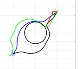
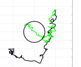
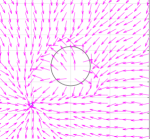
For our empirical evaluation of ZDPG, we consider a two-dimensional continuous state-action navigation problem, where a point agent aims to avoid a spherical (for simplicity) obstacle and converge fast to some fixed target while satisfying its motion control dynamics. This goal is achieved by appropriately shaping the associated reward function. Let sโˆ—โˆˆโ„2superscript๐‘ superscriptโ„2s^{*}\in\mathbb{R}^{2} represent the target the point agent wishes to reach. Let scโˆˆโ„2superscript๐‘ ๐‘superscriptโ„2s^{c}\in\mathbb{R}^{2} and $r\in\mathbb{R}_{+}$ denote the center and radius of the spherical obstacle the agent wishes to avoid. Then, we define the reward $R:\mathbb{R}^{2}\to\mathbb{R}$ as a combination of two artificial potential functions: An attractive potential $\phi^{att}:\mathbb{R}^{2}\to\mathbb{R}_{+}$ with a maximum at the target, and a repulsive artificial potential $\phi^{rep}:\mathbb{R}^{2}\to\mathbb{R}_{+}$ with a minimum at the center of the object. Specifically, we set the attractive potential to be the negative Euclidean distance to the goal location sโˆ—superscript๐‘ s^{*} squared, that is, ฯ•aโ€‹tโ€‹tโ€‹(s):=โˆ’โ€–sโˆ’sโˆ—โ€–22assignsuperscriptitalic-ฯ•๐‘Ž๐‘ก๐‘ก๐‘ superscriptsubscriptnorm๐‘ superscript๐‘ 22\phi^{att}(s):=-\|s-s^{*}\|_{2}^{2}, where s๐‘ s is the location (state) of the agent. Similar to [14], we define the repulsive potential as ฯ•rโ€‹eโ€‹pโ€‹(s):=1โˆ’1/ฮฒโ€‹(s)assignsuperscriptitalic-ฯ•๐‘Ÿ๐‘’๐‘๐‘ 11๐›ฝ๐‘ \phi^{rep}(s):=1-1/\beta(s), where

ฮฒโ€‹(s):=(1โˆ’(1+r4r4)โ‹…(โ€–sโˆ’scโ€–2โˆ’r2)21+(โ€–sโˆ’scโ€–2โˆ’r2)2)12โ€‹(1โˆ’signโ€‹(โ€–sโˆ’scโ€–โˆ’r)).assign๐›ฝ๐‘ superscript1โ‹…1superscript๐‘Ÿ4superscript๐‘Ÿ4superscriptsuperscriptnorm๐‘ superscript๐‘ ๐‘2superscript๐‘Ÿ221superscriptsuperscriptnorm๐‘ superscript๐‘ ๐‘2superscript๐‘Ÿ22121signnorm๐‘ superscript๐‘ ๐‘๐‘Ÿ\beta(s):=\left(1-\left(\frac{1+r^{4}}{r^{4}}\right)\cdot\frac{\left(\|s-s^{c}\|^{2}-r^{2}\right)^{2}}{1+\left(\|s-s^{c}\|^{2}-r^{2}\right)^{2}}\right)^{\frac{1}{2}\left(1-\textrm{sign}\left(\|s-s^{c}\|-r\right)\right)}.

Completely characterized by the state of the agent, the reward is equal to the sum of these attractive and repulsive potentials, that is, Rโ€‹(s)=ฯ•aโ€‹tโ€‹tโ€‹(s)+ฯ•rโ€‹eโ€‹pโ€‹(s)๐‘…๐‘ superscriptitalic-ฯ•๐‘Ž๐‘ก๐‘ก๐‘ superscriptitalic-ฯ•๐‘Ÿ๐‘’๐‘๐‘ R(s)=\phi^{att}(s)+\phi^{rep}(s). Also, the motion dynamics of the point agent are described by the controlled random walk

st+1=Aโ€‹st+ฮทโ€‹ฯ€ฮธโ€‹(st)โ€–ฯ€ฮธโ€‹(st)โ€–+nt,subscript๐‘ ๐‘ก1๐ดsubscript๐‘ ๐‘ก๐œ‚subscript๐œ‹๐œƒsubscript๐‘ ๐‘กnormsubscript๐œ‹๐œƒsubscript๐‘ ๐‘กsubscript๐‘›๐‘กs_{t+1}=As_{t}+\eta\dfrac{\pi_{\theta}(s_{t})}{\|\pi_{\theta}(s_{t})\|}+n_{t}, (8)

where $A\in\mathbb{R}^{2\times 2}$ is the motion state transition matrix of the agent, $\{n_{t}\}$ is a random process modeling state process noise, and $\eta>0$ (together with policy normalization) imposes implicit resource constraints on the agent motion. Here, we assume that, except from the agent control vector (second term on the right-hand side of (8)), the dynamics of the agent are unknown, an assumption which conforms with the standard policy gradient setting. Lastly, we consider a linear, deterministic policy to determine optimal directions that the point agent will follow given its location to its prescribed destination. In particular, we adopt a Radial-Basis-Function (RBF) expansion as our (universal) policy parameterization, i.e.,

ฯ€ฮธโ€‹(s)=โˆ‘i=1dฮธiโ€‹ฮบโ€‹(s,sยฏi),subscript๐œ‹๐œƒ๐‘ superscriptsubscript๐‘–1๐‘‘subscript๐œƒ๐‘–๐œ…๐‘ subscriptยฏ๐‘ ๐‘–\pi_{\theta}(s)=\sum_{i=1}^{d}\theta_{i}\kappa(s,\bar{s}_{i}), (9)

where ฮบโ€‹(s,sโ€ฒ)=expโ€‹(โˆ’โ€–sโˆ’sโ€ฒโ€–22/2โ€‹ฯƒฮบ2)๐œ…๐‘ superscript๐‘ โ€ฒexpsubscriptsuperscriptnorm๐‘ superscript๐‘ โ€ฒ222superscriptsubscript๐œŽ๐œ…2\kappa(s,s^{\prime})=\textrm{exp}(-\|s-s^{\prime}\|^{2}_{2}/2\sigma_{\kappa}^{2}) defines the RBF kernel, $\theta_{i}\in\mathbb{R}^{2},i=1,\dots,d$ are the parameter vectors to be learned, $\sigma_{\kappa}^{2}$ determines the variance of the kernel, and sยฏi,i=1,โ€ฆ,dformulae-sequencesubscriptยฏ๐‘ ๐‘–๐‘–1โ€ฆ๐‘‘\bar{s}_{i},i=1,\dots,d are the associated RBF centers.

For all simulations, we select the target of the agent to be located at sโˆ—=(โˆ’5,โˆ’5)superscript๐‘ 55s^{*}=(-5,-5), and the obstacle to be centered at sc=(0,0)superscript๐‘ ๐‘00s^{c}=(0,0) with a radius of $r=2.5$. We define the potential with a slightly larger radius ($r=3$) to ensure that the agent does not collide with the boundary of the obstacle. We select the centers of the RBF kernels to be spaced $0.25$ units from each other populating the $[-10,10]\times[-10,10]$ grid. The initial state distribution is uniform on $[-10,10]\times[-10,10]$.

5.2 Results

ย ย ย Refer to caption ย ย ย  Refer to caption ย ย ย  Refer to caption
(a) (b) (c)
Figure 1: Average reward per episode with confidence bounds over 50 trials. Learning rate set to $\alpha=10^{-7}$ for all simulations. (a) Noiseless case with no MC variance reduction ($N=1$), ZDPG and ZDPG-S smoothing parameters set to $0.05$ and $0.5$ respectively. Action noise for PG and PG-B set to $\sigma_{a}^{2}=0.025$. (b) Noisy case ($\omega=0.01$) with no MC reduction ($N=1$), ZDPG and ZDPG-S smoothing parameters set to $0.25$ and $0.5$ respectively. Action noise for PG and PG-B set to $\sigma_{a}^{2}=0.025$. (c) Noisy case (same as (b)) with MC reduction ($N=10$).

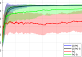
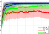
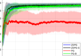
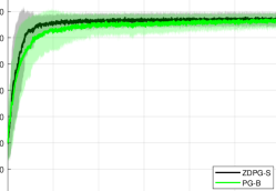
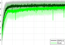
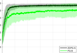
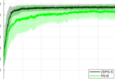
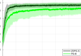
The learning curves shown in Figure 1 illustrate the performance of ZDPG and its symmetric counterpart ZDPG-S (based on (6)), compared with PG and PG with a stochastic baseline (PG-B), with discount factor $\gamma=0.8$ in the case with and without system noise ($n_{t}=\mathbf{0}$ and $n_{t}\sim\mathcal{N}(\mathbf{0},\omega\cdot I_{2})$, respectively). Also, we set $A=I_{2}$. For PG and PG-B, we let $\tilde{\pi}$ denote the stochastic policy where the action is selected by atโˆผฯ€~ฮธโ€‹(st)similar-tosubscript๐‘Ž๐‘กsubscript~๐œ‹๐œƒsubscript๐‘ ๐‘กa_{t}\sim\tilde{\pi}_{\theta}(s_{t}). In particular, we let $\tilde{\pi}$ be a Gaussian policy with mean equal to ฯ€ฮธโ€‹(s)subscript๐œ‹๐œƒ๐‘ \pi_{\theta}(s) [c.f. (9)] and a standard choice of covariance matrix $\Sigma=\sigma_{a}^{2}\cdot I_{2}$. For PG-B, the baseline is fairly chosen and is analogous as compared to ZDPG in that it scales the update direction โˆ‡ฮธlogโกฯ€~ฮธโ€‹(s)subscriptโˆ‡๐œƒsubscript~๐œ‹๐œƒ๐‘ \nabla_{\theta}\log\tilde{\pi}_{\theta}(s) by a two-point difference (Q^โ€‹(s,a)โˆ’V~โ€‹(s)^๐‘„๐‘ ๐‘Ž~๐‘‰๐‘ \hat{Q}(s,a)-\tilde{V}(s)), where V~โ€‹(s)~๐‘‰๐‘ \tilde{V}(s) is a single-rollout estimate of the associated value function at state s๐‘ s. After each policy update, we evaluate the system by generating a rollout of fixed length $T=20$ from a fixed starting point s0=(5,5)superscript๐‘ 055s^{0}=(5,5). As done commonly in practice (as a heuristic), we evaluate the stochastic policies by setting the covariance matrix equal to zero thereby making the evaluation policy deterministic.

โ€… Refer to caption ย ย ย ย ย ย  Refer to caption ย ย ย ย ย ย  Refer to caption
(a) (b) (c)
Figure 2: Sample trajectories with fixed length $T=100$ of learned policies corresponding to noiseless ((a): $N=1$, $\omega=0$) and noisy ((b): $N=10$, $\omega=0.1$) settings (c) Learned field plot for ZDPG-S with noise level $\omega=0.1$ shows that the variance in Figure 1 comes only from the system noise.

Depending on the level of the system noise, ZDPG(-S) consistently outperforms PG-B (and also PG), both in mean performance and the associated variance. Interestingly, the improvement of ZDPG over PG-B is sharper when the agent dynamics are noisy (also see our Supplementary Material, Section E). In fact, we observe that, either with or without system noise, the perturbation of the initial state with a deterministic policy indeed provides more meaningful information for policy improvement than in the setting of a stochastic policy (also see Figure 2). One should also note that PG-B performs better in the noisy setting with MC variance reduction (1 (c)) than the noiseless setting (1 (a)). Indeed, variance reduction improves the performance of all methods, except for vanilla policy gradient. We emphasize though that we evaluate stochastic policies using only their means. Our empirical results corroborate the claim that randomness in the policy is not necessary to solve MDPs within the PG-based RL framework.

6 Conclusions and Future Work

In this work, we introduced the ZDPG algorithm, which is based on an efficient two-point zeroth-order approximation of the deterministic policy gradient, for the infinite horizon Markov decision problem. Using random horizons to evaluate the zeroth-order estimates of the state-action function, we showed that low-dimensional perturbations in the action space can effectively replace the need for randomized policies in the classical policy gradient setting. We also presented finite sample complexity results for ZDPG, which improve upon the state of the art by up to two orders of magnitude. Finally, we corroborated our results with a numerical evaluation on a navigation problem which showcased the advantages of ZDPG over both standard PG and PG with a baseline. For future work, variance reduced ZDPG could be realized with more sample efficient variance reduction techniques, such as gradient averaging or using a critic network to evaluate zeroth order state action function.

References

  • [1] Kai Arulkumaran, Marcย Peter Deisenroth, Miles Brundage, and Anilย Anthony Bharath. Deep reinforcement learning: A brief survey. IEEE Signal Processing Magazine, 34(6):26โ€“38, 2017.
  • [2] Jalaj Bhandari, Daniel Russo, and Raghav Singal. A finite time analysis of temporal difference learning with linear function approximation. arXiv preprint arXiv:1806.02450, 2018.
  • [3] Gal Dalal, Balรกzs Szรถrรฉnyi, Gugan Thoppe, and Shie Mannor. Finite sample analyses for td (0) with function approximation. In Thirty-Second AAAI Conference on Artificial Intelligence, 2018.
  • [4] Johnย C Duchi, Michaelย I Jordan, Martinย J Wainwright, and Andre Wibisono. Optimal rates for zero-order convex optimization: The power of two function evaluations. IEEE Transactions on Information Theory, 61(5):2788โ€“2806, 2015.
  • [5] Mark Eisen, Clark Zhang, Luizย FO Chamon, Danielย D Lee, and Alejandro Ribeiro. Learning optimal resource allocations in wireless systems. IEEE Transactions on Signal Processing, 67(10):2775โ€“2790, 2019.
  • [6] Maryam Fazel, Rong Ge, Shamย M Kakade, and Mehran Mesbahi. Global convergence of policy gradient methods for the linear quadratic regulator. arXiv preprint arXiv:1801.05039, 2018.
  • [7] Scott Fujimoto, Herke Vanย Hoof, and David Meger. Addressing function approximation error in actor-critic methods. arXiv preprint arXiv:1802.09477, 2018.
  • [8] Saeed Ghadimi and Guanghui Lan. Stochastic first-and zeroth-order methods for nonconvex stochastic programming. SIAM Journal on Optimization, 23(4):2341โ€“2368, 2013.
  • [9] Saeed Ghadimi, Guanghui Lan, and Hongchao Zhang. Mini-batch stochastic approximation methods for nonconvex stochastic composite optimization. Mathematical Programming, 155(1-2):267โ€“305, 2016.
  • [10] Ilaria Giannoccaro and Pierpaolo Pontrandolfo. Inventory management in supply chains: a reinforcement learning approach. International Journal of Production Economics, 78(2):153โ€“161, 2002.
  • [11] Evan Greensmith, Peterย L Bartlett, and Jonathan Baxter. Variance reduction techniques for gradient estimates in reinforcement learning. Journal of Machine Learning Research, 5(Nov):1471โ€“1530, 2004.
  • [12] Shixiang Gu, Ethan Holly, Timothy Lillicrap, and Sergey Levine. Deep reinforcement learning for robotic manipulation with asynchronous off-policy updates. In 2017 IEEE international conference on robotics and automation (ICRA), pages 3389โ€“3396. IEEE, 2017.
  • [13] Dionysiosย S Kalogerias, Mark Eisen, Georgeย J Pappas, and Alejandro Ribeiro. Model-free learning of optimal ergodic policies in wireless systems. arXiv preprint arXiv:1911.03988, 2019.
  • [14] Dionysiosย S Kalogerias and Athinaย P Petropulu. Mobi-cliques for improving ergodic secrecy in fading wiretap channels under power constraints. In 2014 IEEE International Conference on Acoustics, Speech and Signal Processing (ICASSP), pages 1578โ€“1591. IEEE, 2014.
  • [15] Dionysiosย S Kalogerias and Warrenย B Powell. Zeroth-order stochastic compositional algorithms for risk-aware learning. arXiv preprint arXiv:1912.09484, 2019.
  • [16] Jens Kober, Jย Andrew Bagnell, and Jan Peters. Reinforcement learning in robotics: A survey. The International Journal of Robotics Research, 32(11):1238โ€“1274, 2013.
  • [17] Vijayย R Konda and Johnย N Tsitsiklis. Onactor-critic algorithms. SIAM journal on Control and Optimization, 42(4):1143โ€“1166, 2003.
  • [18] Harshat Kumar, Alec Koppel, and Alejandro Ribeiro. On the sample complexity of actor-critic method for reinforcement learning with function approximation. arXiv preprint arXiv:1910.08412, 2019.
  • [19] Timothyย P Lillicrap, Jonathanย J Hunt, Alexander Pritzel, Nicolas Heess, Tom Erez, Yuval Tassa, David Silver, and Daan Wierstra. Continuous control with deep reinforcement learning. arXiv preprint arXiv:1509.02971, 2015.
  • [20] Dhruv Malik, Ashwin Pananjady, Kush Bhatia, Koulik Khamaru, Peterย L Bartlett, and Martinย J Wainwright. Derivative-free methods for policy optimization: Guarantees for linear quadratic systems. Journal of Machine Learning Research, 21(21):1โ€“51, 2020.
  • [21] Hesameddin Mohammadi, Armin Zare, Mahdi Soltanolkotabi, and Mihailoย R Jovanoviฤ‡. Convergence and sample complexity of gradient methods for the model-free linear quadratic regulator problem. arXiv preprint arXiv:1912.11899, 2019.
  • [22] Yurii Nesterov and Vladimir Spokoiny. Random gradient-free minimization of convex functions. Foundations of Computational Mathematics, 17(2):527โ€“566, 2017.
  • [23] Andrewย Y Ng, Daishi Harada, and Stuart Russell. Policy invariance under reward transformations: Theory and application to reward shaping. In ICML, volumeย 99, pages 278โ€“287, 1999.
  • [24] Matteo Papini, Damiano Binaghi, Giuseppe Canonaco, Matteo Pirotta, and Marcello Restelli. Stochastic variance-reduced policy gradient. arXiv preprint arXiv:1806.05618, 2018.
  • [25] Santiago Paternain, Juanย Andrรฉs Bazerque, Austin Small, and Alejandro Ribeiro. Stochastic policy gradient ascent in reproducing kernel hilbert spaces. arXiv preprint arXiv:1807.11274, 2018.
  • [26] Matteo Pirotta, Marcello Restelli, and Luca Bascetta. Policy gradient in lipschitz markov decision processes. Machine Learning, 100(2-3):255โ€“283, 2015.
  • [27] John Schulman, Sergey Levine, Pieter Abbeel, Michael Jordan, and Philipp Moritz. Trust region policy optimization. In International conference on machine learning, pages 1889โ€“1897, 2015.
  • [28] David Silver, Aja Huang, Chrisย J Maddison, Arthur Guez, Laurent Sifre, George Van Denย Driessche, Julian Schrittwieser, Ioannis Antonoglou, Veda Panneershelvam, Marc Lanctot, etย al. Mastering the game of go with deep neural networks and tree search. nature, 529(7587):484, 2016.
  • [29] David Silver, Guy Lever, Nicolas Heess, Thomas Degris, Daan Wierstra, and Martin Riedmiller. Deterministic policy gradient algorithms. In Proceedings of the 31st International Conference on International Conference on Machine Learning - Volume 32, ICMLโ€™14, page Iโ€“387โ€“Iโ€“395. JMLR.org, 2014.
  • [30] Richardย S Sutton, Davidย A McAllester, Satinderย P Singh, and Yishay Mansour. Policy gradient methods for reinforcement learning with function approximation. In Advances in neural information processing systems, pages 1057โ€“1063, 2000.
  • [31] Gerald Tesauro. Temporal difference learning and td-gammon. Communications of the ACM, 38(3):58โ€“68, 1995.
  • [32] Anirudh Vemula, Wen Sun, and Jย Andrew Bagnell. Contrasting exploration in parameter and action space: A zeroth-order optimization perspective. arXiv preprint arXiv:1901.11503, 2019.
  • [33] Linย F Yang and Mengdi Wang. Reinforcement leaning in feature space: Matrix bandit, kernels, and regret bound. arXiv preprint arXiv:1905.10389, 2019.
  • [34] Hao Ye, Geoffreyย Ye Li, and Biing-Hwangย Fred Juang. Deep reinforcement learning based resource allocation for v2v communications. IEEE Transactions on Vehicular Technology, 68(4):3163โ€“3173, 2019.
  • [35] Kaiqing Zhang, Alec Koppel, Hao Zhu, and Tamer BaลŸar. Global convergence of policy gradient methods to (almost) locally optimal policies. arXiv preprint arXiv:1906.08383, 2019.

Supplementary Material

Appendix A Proof of Lemma 2

Since the estimate $\hat{Q}$ is unbiased, it suffices to show that $\mathbb{E}[|\hat{Q}|^{2}]$ is bounded. Indeed, we have

๐”ผโ€‹[|Q^|2]=๐”ผโ€‹[|โˆ‘t=0TRโ€‹(st,at=ฯ€ฮธโ€‹(st))|2]๐”ผdelimited-[]superscript^๐‘„2๐”ผdelimited-[]superscriptsuperscriptsubscript๐‘ก0๐‘‡๐‘…subscript๐‘ ๐‘กsubscript๐‘Ž๐‘กsubscript๐œ‹๐œƒsubscript๐‘ ๐‘ก2\displaystyle\mathbb{E}[|\hat{Q}|^{2}]=\mathbb{E}\Bigg{[}\Bigg{|}\sum_{t=0}^{T}R(s_{t},a_{t}=\pi_{\theta}(s_{t}))\Bigg{|}^{2}\Bigg{]} โ‰ค๐”ผโ€‹[(โˆ‘t=0T|Rโ€‹(st,at=ฯ€ฮธโ€‹(st))|)2]absent๐”ผdelimited-[]superscriptsuperscriptsubscript๐‘ก0๐‘‡๐‘…subscript๐‘ ๐‘กsubscript๐‘Ž๐‘กsubscript๐œ‹๐œƒsubscript๐‘ ๐‘ก2\displaystyle\leq\mathbb{E}\Bigg{[}\Bigg{(}\sum_{t=0}^{T}|R(s_{t},a_{t}=\pi_{\theta}(s_{t}))|\Bigg{)}^{2}\Bigg{]}
$\displaystyle\leq\mathbb{E}\big{[}(T+1)^{2}U_{R}^{2}\big{]}=U_{R}^{2}\dfrac{1+\gamma}{(1-\gamma)^{2}},$

where the last equality follows from the fact that $T$ is a geometric random variable with probability of success $1-\gamma$. Enough said. $\square$

Appendix B Proof of Theorem 1

Let Assumptions 1-3 and also Assumption 4 be in effect. Also, recall the definitions of the gradients, namely

โˆ‡Jโ€‹(ฮธ)=๐”ผsโˆผฯฯ€ฮธโ€‹[โˆ‡ฮธฯ€ฮธโ€‹(s)โ€‹โˆ‡aQฯ€ฮธโ€‹(s,a)|a=ฯ€ฮธโ€‹(s)],โˆ‡๐ฝ๐œƒsubscript๐”ผsimilar-to๐‘ superscript๐œŒsubscript๐œ‹๐œƒdelimited-[]evaluated-atsubscriptโˆ‡๐œƒsubscript๐œ‹๐œƒ๐‘ subscriptโˆ‡๐‘Žsuperscript๐‘„subscript๐œ‹๐œƒ๐‘ ๐‘Ž๐‘Žsubscript๐œ‹๐œƒ๐‘ \nabla J(\theta)=\mathbb{E}_{s\sim\rho^{\pi_{\theta}}}\left[\nabla_{\theta}\pi_{\theta}(s)\nabla_{a}Q^{\pi_{\theta}}(s,a)|_{a=\pi_{\theta}(s)}\right],

and

โˆ‡^โ€‹Jโ€‹(ฮธ)=๐”ผsโˆผฯฯ€ฮธโ€‹[โˆ‡ฮธฯ€ฮธโ€‹(s)โ€‹โˆ‡aQฮผฯ€ฮธโ€‹(s,a)|a=ฯ€ฮธโ€‹(s)].^โˆ‡๐ฝ๐œƒsubscript๐”ผsimilar-to๐‘ superscript๐œŒsubscript๐œ‹๐œƒdelimited-[]evaluated-atsubscriptโˆ‡๐œƒsubscript๐œ‹๐œƒ๐‘ subscriptโˆ‡๐‘Žsuperscriptsubscript๐‘„๐œ‡subscript๐œ‹๐œƒ๐‘ ๐‘Ž๐‘Žsubscript๐œ‹๐œƒ๐‘ \hat{\nabla}J(\theta)=\mathbb{E}_{s\sim\rho^{\pi_{\theta}}}\left[\nabla_{\theta}\pi_{\theta}(s)\nabla_{a}Q_{\mu}^{\pi_{\theta}}(s,a)|_{a=\pi_{\theta}(s)}\right].

By definition, and then by Jensen, we have

$$\begin{split}\|\nabla J(\theta)&-\hat{\nabla}J(\theta)\|\\ &=\Big{\|}\mathbb{E}_{s\sim\rho^{\pi_{\theta}}}\left[\nabla_{\theta}\pi_{\theta}(s)\nabla_{a}Q^{\pi_{\theta}}(s,a)\big{|}_{a=\pi_{\theta}(s)}\right]-\mathbb{E}_{s\sim\rho^{\pi_{\theta}}}\left[\nabla_{\theta}\pi_{\theta}(s)\nabla_{a}Q_{\mu}^{\pi_{\theta}}(s,a)\big{|}_{a=\pi_{\theta}(s)}\right]\Big{\|}\\ &=\Big{\|}\mathbb{E}_{s\sim\rho^{\pi_{\theta}}}\left[\nabla_{\theta}\pi_{\theta}(s)\nabla_{a}Q^{\pi_{\theta}}(s,a)\big{|}_{a=\pi_{\theta}(s)}-\nabla_{\theta}\pi_{\theta}(s)\nabla_{a}Q_{\mu}^{\pi_{\theta}}(s,a)\big{|}_{a=\pi_{\theta}(s)}\right]\Big{\|}\\ &\leq\mathbb{E}_{s\sim\rho^{\pi_{\theta}}}\left[\big{\|}\nabla_{\theta}\pi_{\theta}(s)\nabla_{a}Q^{\pi_{\theta}}(s,a)\big{|}_{a=\pi_{\theta}(s)}-\nabla_{\theta}\pi_{\theta}(s)\nabla_{a}Q_{\mu}^{\pi_{\theta}}(s,a)\big{|}_{a=\pi_{\theta}(s)}\big{\|}\right].\end{split}$$

Grouping terms, then applying Cauchy-Schwarz, we obtain

$$\begin{split}\|\nabla J(\theta)-\hat{\nabla}J(\theta)\|&\leq\mathbb{E}_{s\sim\rho^{\pi_{\theta}}}\left[\big{\|}\nabla_{\theta}\pi_{\theta}(s)\big{(}\nabla_{a}Q^{\pi_{\theta}}(s,a)\big{|}_{a=\pi_{\theta}(s)}-\nabla_{a}Q_{\mu}^{\pi_{\theta}}(s,a)\big{|}_{a=\pi_{\theta}(s)}\big{)}\big{\|}\right]\\ &\leq\mathbb{E}_{s\sim\rho^{\pi_{\theta}}}\left[\left\|\nabla_{\theta}\pi_{\theta}(s)\right\|\cdot\left\|\nabla_{a}Q^{\pi_{\theta}}(s,a)\big{|}_{a=\pi_{\theta}(s)}-\nabla_{a}Q_{\mu}^{\pi_{\theta}}(s,a)\big{|}_{a=\pi_{\theta}(s)}\right\|\right].\\ \end{split}$$

By Assumption 1, we can bound โˆ‡ฮธฯ€ฮธโ€‹(s)subscriptโˆ‡๐œƒsubscript๐œ‹๐œƒ๐‘ \nabla_{\theta}\pi_{\theta}(s) by $B_{\Theta}$. As such, the remaining expression can be bounded by invoking Assumption 4, yielding

$$\begin{split}\|\nabla J(\theta)-\hat{\nabla}J(\theta)\|&\leq B_{\Theta}\mathbb{E}_{s\sim\rho^{\pi_{\theta}}}\left[\left\|\nabla_{a}\left(Q^{\pi_{\theta}}(s,a)-Q_{\mu}^{\pi_{\theta}}(s,a)\right)\big{|}_{a=\pi_{\theta}(s)}\right\|\right]\\ &\leq B_{\Theta}\mathbb{E}_{s\sim\rho^{\pi_{\theta}}}\left[\left\|\nabla_{a}\left(Q^{\pi_{\theta}}(s,a)-\mathbb{E}_{\mathbf{u}}\left[Q^{\pi_{\theta}}(s,a+\mu\textbf{u})\right]\right)\big{|}_{a=\pi_{\theta}(s)}\right\|\right]\\ &\leq B_{\Theta}\mathbb{E}_{s\sim\rho^{\pi_{\theta}}}\left[\left\|\nabla_{a}\left(\mathbb{E}_{\mathbf{u}}\left[Q^{\pi_{\theta}}(s,a)-Q^{\pi_{\theta}}(s,a+\mu\textbf{u})\right]\right)\big{|}_{a=\pi_{\theta}(s)}\right\|\right]\\ &\leq B_{\Theta}\mathbb{E}_{s\sim\rho^{\pi_{\theta}}}\left[\left\|\mathbb{E}_{\mathbf{u}}\left[\nabla_{a}\left(Q^{\pi_{\theta}}(s,a)-Q^{\pi_{\theta}}(s,a+\mu\textbf{u})\right]\right)\big{|}_{a=\pi_{\theta}(s)}\right\|\right]\\ &\leq B_{\Theta}\mathbb{E}_{s\sim\rho^{\pi_{\theta}}}\left[\mathbb{E}_{\mathbf{u}}\left[\left\|\nabla_{a}\left(Q^{\pi_{\theta}}(s,a)-Q^{\pi_{\theta}}(s,a+\mu\textbf{u})\right)\big{|}_{a=\pi_{\theta}(s)}\right\|\right]\right]\\ &\leq B_{\Theta}\mathbb{E}_{s\sim\rho^{\pi_{\theta}}}\left[\mathbb{E}_{\mathbf{u}}\left[G\left\|\mu\mathbf{u}\right\|\right]\right]\\ &\leq B_{\Theta}\mu\sqrt{p}G/(1-\gamma),\end{split}$$

where the final inequality comes from [22, Lemma 1].

If, alternatively, Assumption 5 instead of Assumption 4, holds, then by [22, Lemma 3], we obtain

$$\begin{split}\|\nabla J(\theta)-\hat{\nabla}J(\theta)\|&\leq B_{\Theta}\mathbb{E}_{s\sim\rho^{\pi_{\theta}}}\left[\left\|\nabla_{a}\left(Q^{\pi_{\theta}}(s,a)-Q_{\mu}^{\pi_{\theta}}(s,a)\right)\big{|}_{a=\pi_{\theta}(s)}\right\|\right]\\ &\leq B_{\Theta}\mu^{2}(p+4)^{2}H/(1-\gamma).\end{split}$$

This completes the proof. $\square$

Appendix C Proof of Lemma 3

First, by definition, we may write

$$(1-\gamma)^{2}\mathbb{E}[\|g_{t}\|^{2}]=\mathbb{E}\Bigg{[}\Bigg{\|}\nabla_{\theta}\pi_{\theta_{t}}(s_{t})\dfrac{\hat{Q}_{t}^{+}-\hat{Q}_{t}^{-}}{\mu}{\bf u}\Bigg{\|}^{2}\Bigg{]}=:\mathbb{E}[\|g^{\prime}_{t}\|^{2}],$$

where

$\displaystyle\hat{Q}_{t}^{\pm}$ $\displaystyle=Q^{\pi_{\theta_{t}}}(\pm)+\dfrac{1}{N}\sum_{n=1}^{N}w_{t,n}^{\pm}.$

By Cauchy-Schwarz, and by exploiting the above, we readily get

$\displaystyle\mathbb{E}[\|g^{\prime}_{t}\|^{2}]$ $\displaystyle\leq B_{\Theta}^{2}\mathbb{E}\Bigg{[}\Bigg{\|}\dfrac{Q^{\pi_{\theta_{t}}}(+)-Q^{\pi_{\theta_{t}}}(-)}{\mu}+\dfrac{1}{N}\sum_{n=1}^{N}\dfrac{w_{t,n}^{+}-w_{t,n}^{-}}{\mu}\Bigg{\|}^{2}\|{\bf u}\|^{2}\Bigg{]}$
=Bฮ˜2โ€‹๐”ผโ€‹[|Qฯ€ฮธtโ€‹(st,ฯ€ฮธtโ€‹(st)+ฮผโ€‹๐ฎ)โˆ’Qฯ€ฮธtโ€‹(st,ฯ€ฮธtโ€‹(st))ฮผ+1Nโ€‹โˆ‘n=1Nwt,n+โˆ’wt,nโˆ’ฮผ|2โ€‹โ€–๐ฎโ€–2]absentsuperscriptsubscript๐ตฮ˜2๐”ผdelimited-[]superscriptsuperscript๐‘„subscript๐œ‹subscript๐œƒ๐‘กsubscript๐‘ ๐‘กsubscript๐œ‹subscript๐œƒ๐‘กsubscript๐‘ ๐‘ก๐œ‡๐ฎsuperscript๐‘„subscript๐œ‹subscript๐œƒ๐‘กsubscript๐‘ ๐‘กsubscript๐œ‹subscript๐œƒ๐‘กsubscript๐‘ ๐‘ก๐œ‡1๐‘superscriptsubscript๐‘›1๐‘superscriptsubscript๐‘ค๐‘ก๐‘›superscriptsubscript๐‘ค๐‘ก๐‘›๐œ‡2superscriptnorm๐ฎ2\displaystyle=B_{\Theta}^{2}\mathbb{E}\Bigg{[}\Bigg{|}\dfrac{Q^{\pi_{\theta_{t}}}(s_{t},\pi_{\theta_{t}}(s_{t})+\mu{\bf u})-Q^{\pi_{\theta_{t}}}(s_{t},\pi_{\theta_{t}}(s_{t}))}{\mu}+\dfrac{1}{N}\sum_{n=1}^{N}\dfrac{w_{t,n}^{+}-w_{t,n}^{-}}{\mu}\Bigg{|}^{2}\|{\bf u}\|^{2}\Bigg{]}
$\displaystyle\leq 2B_{\Theta}^{2}\mathbb{E}\Bigg{[}\Bigg{|}\dfrac{Q^{\pi_{\theta_{t}}}(s_{t},\pi_{\theta_{t}}(s_{t})+\mu{\bf u})-Q^{\pi_{\theta_{t}}}(s_{t},\pi_{\theta_{t}}(s_{t}))}{\mu}\Bigg{|}^{2}\|{\bf u}\|^{2}$
$\displaystyle\quad\quad\quad\quad\quad\quad\quad\quad\quad\quad\quad\quad\quad\quad\quad\quad\quad\quad+\Bigg{|}\dfrac{1}{N}\sum_{n=1}^{N}\dfrac{w_{t,n}^{+}-w_{t,n}^{-}}{\mu}\Bigg{|}^{2}\|{\bf u}\|^{2}\Bigg{]}.$ (10)

For the first term on the right-hand side of (10), we have

๐”ผโ€‹[|Qฯ€ฮธtโ€‹(st,ฯ€ฮธtโ€‹(st)+ฮผโ€‹๐ฎ)โˆ’Qฯ€ฮธtโ€‹(st,ฯ€ฮธtโ€‹(st))ฮผ|2โ€‹โ€–๐ฎโ€–2]โ‰คL2โ€‹๐”ผโ€‹[โ€–๐ฎโ€–4]โ‰คL2โ€‹(p+4)2.๐”ผdelimited-[]superscriptsuperscript๐‘„subscript๐œ‹subscript๐œƒ๐‘กsubscript๐‘ ๐‘กsubscript๐œ‹subscript๐œƒ๐‘กsubscript๐‘ ๐‘ก๐œ‡๐ฎsuperscript๐‘„subscript๐œ‹subscript๐œƒ๐‘กsubscript๐‘ ๐‘กsubscript๐œ‹subscript๐œƒ๐‘กsubscript๐‘ ๐‘ก๐œ‡2superscriptnorm๐ฎ2superscript๐ฟ2๐”ผdelimited-[]superscriptnorm๐ฎ4superscript๐ฟ2superscript๐‘42\mathbb{E}\Bigg{[}\Bigg{|}\dfrac{Q^{\pi_{\theta_{t}}}(s_{t},\pi_{\theta_{t}}(s_{t})+\mu{\bf u})-Q^{\pi_{\theta_{t}}}(s_{t},\pi_{\theta_{t}}(s_{t}))}{\mu}\Bigg{|}^{2}\|{\bf u}\|^{2}\Bigg{]}\leq L^{2}\mathbb{E}\big{[}\|{\bf u}\|^{4}\big{]}\leq L^{2}(p+4)^{2}. (11)

For the second term on the right-hand side of (10), we may write

$\displaystyle\mathbb{E}\Bigg{[}\Bigg{|}\dfrac{1}{N}\sum_{n=1}^{N}\dfrac{w_{t,n}^{+}-w_{t,n}^{-}}{\mu}\Bigg{|}^{2}\|{\bf u}\|^{2}\Bigg{]}$ =1ฮผ2โ€‹N2โ€‹๐”ผโ€‹[๐”ผโ€‹[|โˆ‘n=1Nwt,n+โˆ’wt,nโˆ’|2โ€‹โ€–๐ฎโ€–2|st,๐ฎ,ฮธt,TQ]]absent1superscript๐œ‡2superscript๐‘2๐”ผdelimited-[]๐”ผdelimited-[]conditionalsuperscriptsuperscriptsubscript๐‘›1๐‘superscriptsubscript๐‘ค๐‘ก๐‘›superscriptsubscript๐‘ค๐‘ก๐‘›2superscriptnorm๐ฎ2subscript๐‘ ๐‘ก๐ฎsubscript๐œƒ๐‘กsubscript๐‘‡๐‘„\displaystyle=\dfrac{1}{\mu^{2}N^{2}}\mathbb{E}\Bigg{[}\mathbb{E}\Bigg{[}\Bigg{|}\sum_{n=1}^{N}w_{t,n}^{+}-w_{t,n}^{-}\Bigg{|}^{2}\|{\bf u}\|^{2}\Bigg{|}s_{t},{\bf u},\theta_{t},T_{Q}\Bigg{]}\Bigg{]}
=1ฮผ2โ€‹N2โ€‹๐”ผโ€‹[โ€–๐ฎโ€–2โ€‹๐”ผโ€‹[|โˆ‘n=1Nwt,n+โˆ’wt,nโˆ’|2|st,๐ฎ,ฮธt,TQ]].absent1superscript๐œ‡2superscript๐‘2๐”ผdelimited-[]superscriptnorm๐ฎ2๐”ผdelimited-[]conditionalsuperscriptsuperscriptsubscript๐‘›1๐‘superscriptsubscript๐‘ค๐‘ก๐‘›superscriptsubscript๐‘ค๐‘ก๐‘›2subscript๐‘ ๐‘ก๐ฎsubscript๐œƒ๐‘กsubscript๐‘‡๐‘„\displaystyle=\dfrac{1}{\mu^{2}N^{2}}\mathbb{E}\Bigg{[}\|{\bf u}\|^{2}\mathbb{E}\Bigg{[}\Bigg{|}\sum_{n=1}^{N}w_{t,n}^{+}-w_{t,n}^{-}\Bigg{|}^{2}\Bigg{|}s_{t},{\bf u},\theta_{t},T_{Q}\Bigg{]}\Bigg{]}.

Naturally, we need to focus on the (inner) conditional expectation above. By construction, it is true that, for every $t$, the differences $w_{t,n}^{+}-w_{t,n}^{-},n\in\mathbb{N}_{N}^{+}$ are conditionally independent and identically distributed relative to s,๐ฎ,ฮธt๐‘ ๐ฎsubscript๐œƒ๐‘กs,{\bf u},\theta_{t} and $T_{Q}$, and with zero mean. This implies that

๐”ผโ€‹[|โˆ‘n=1Nwt,n+โˆ’wt,nโˆ’|2|st,๐ฎ,ฮธt,TQ]๐”ผdelimited-[]conditionalsuperscriptsuperscriptsubscript๐‘›1๐‘superscriptsubscript๐‘ค๐‘ก๐‘›superscriptsubscript๐‘ค๐‘ก๐‘›2subscript๐‘ ๐‘ก๐ฎsubscript๐œƒ๐‘กsubscript๐‘‡๐‘„\displaystyle\mathbb{E}\Bigg{[}\Bigg{|}\sum_{n=1}^{N}w_{t,n}^{+}-w_{t,n}^{-}\Bigg{|}^{2}\Bigg{|}s_{t},{\bf u},\theta_{t},T_{Q}\Bigg{]} =โˆ‘n=1N๐”ผโ€‹[|wt,n+โˆ’wt,nโˆ’|2|st,๐ฎ,ฮธt,TQ]absentsuperscriptsubscript๐‘›1๐‘๐”ผdelimited-[]conditionalsuperscriptsuperscriptsubscript๐‘ค๐‘ก๐‘›superscriptsubscript๐‘ค๐‘ก๐‘›2subscript๐‘ ๐‘ก๐ฎsubscript๐œƒ๐‘กsubscript๐‘‡๐‘„\displaystyle=\sum_{n=1}^{N}\mathbb{E}\big{[}\big{|}w_{t,n}^{+}-w_{t,n}^{-}\big{|}^{2}\big{|}s_{t},{\bf u},\theta_{t},T_{Q}\big{]}
=Nโ€‹๐”ผโ€‹[|wt,1+โˆ’wt,1โˆ’|2|st,๐ฎ,ฮธt,TQ],absent๐‘๐”ผdelimited-[]conditionalsuperscriptsuperscriptsubscript๐‘ค๐‘ก1superscriptsubscript๐‘ค๐‘ก12subscript๐‘ ๐‘ก๐ฎsubscript๐œƒ๐‘กsubscript๐‘‡๐‘„\displaystyle=N\mathbb{E}\big{[}\big{|}w_{t,1}^{+}-w_{t,1}^{-}\big{|}^{2}\big{|}s_{t},{\bf u},\theta_{t},T_{Q}\big{]},
โ‰คNโ€‹2โ€‹๐”ผโ€‹[(wt,1+)2+(wt,1โˆ’)2|st,๐ฎ,ฮธt,TQ]absent๐‘2๐”ผdelimited-[]superscriptsuperscriptsubscript๐‘ค๐‘ก12conditionalsuperscriptsuperscriptsubscript๐‘ค๐‘ก12subscript๐‘ ๐‘ก๐ฎsubscript๐œƒ๐‘กsubscript๐‘‡๐‘„\displaystyle\leq N2\mathbb{E}\big{[}\big{(}w_{t,1}^{+}\big{)}^{2}+\big{(}w_{t,1}^{-}\big{)}^{2}\big{|}s_{t},{\bf u},\theta_{t},T_{Q}\big{]}
$\displaystyle\leq N4U_{R}^{2}\dfrac{1+\gamma}{(1-\gamma)^{2}}=:N\sigma^{2},$

where in the last line we have used Lemma 2 twice. As a result, we obtain that

$$\mathbb{E}\Bigg{[}\Bigg{|}\dfrac{1}{N}\sum_{n=1}^{N}\dfrac{w_{t,n}^{+}-w_{t,n}^{-}}{\mu}\Bigg{|}^{2}\|{\bf u}\|^{2}\Bigg{]}\leq\dfrac{\sigma^{2}p}{\mu^{2}N},$$ (12)

since $\mathbb{E}\big{[}\|{\bf u}\|^{2}\big{]}\equiv p$. Combining (11) and (12), we end up with the uniform bound

$$\mathbb{E}[\|g_{t}\|^{2}]\leq\dfrac{2B_{\Theta}^{2}}{(1-\gamma)^{2}}\Big{(}L^{2}(p+4)^{2}+\dfrac{\sigma^{2}p}{\mu^{2}N}\Big{)},$$

thus completing the proof. $\square$

Appendix D Proof of Theorem 2

First, it is not hard to see that the stochastic ascend direction $g_{t}$ constructed by Algorithm 1 is an unbiased estimate of the quasi-gradient $\hat{\nabla}J$. Indeed, with stโˆผ(1โˆ’ฮณ)โ€‹ฯฯ€ฮธtsimilar-tosubscript๐‘ ๐‘ก1๐›พsuperscript๐œŒsubscript๐œ‹subscript๐œƒ๐‘กs_{t}\sim(1-\gamma)\rho^{\pi_{\theta_{t}}}, we may carefully write

$\displaystyle(1-\gamma)\mathbb{E}[g_{t}|\theta_{t}]$ =๐”ผโ€‹[โˆ‡ฮธฯ€ฮธtโ€‹(st)โ€‹Q^t+โˆ’Q^tโˆ’ฮผโ€‹๐ฎ|ฮธt]absent๐”ผdelimited-[]conditionalsubscriptโˆ‡๐œƒsubscript๐œ‹subscript๐œƒ๐‘กsubscript๐‘ ๐‘กsuperscriptsubscript^๐‘„๐‘กsuperscriptsubscript^๐‘„๐‘ก๐œ‡๐ฎsubscript๐œƒ๐‘ก\displaystyle=\mathbb{E}\Bigg{[}\nabla_{\theta}\pi_{\theta_{t}}(s_{t})\dfrac{\hat{Q}_{t}^{+}-\hat{Q}_{t}^{-}}{\mu}{\bf u}\Bigg{|}\theta_{t}\Bigg{]}
=๐”ผโ€‹[๐”ผโ€‹[โˆ‡ฮธฯ€ฮธtโ€‹(st)โ€‹Q^t+โ€‹(st,๐ฎ,ฮธt,TQ)โˆ’Q^tโˆ’โ€‹(st,ฮธt,TQ)ฮผโ€‹๐ฎ|st,๐ฎ,ฮธt,TQ]|ฮธt]absent๐”ผdelimited-[]conditional๐”ผdelimited-[]conditionalsubscriptโˆ‡๐œƒsubscript๐œ‹subscript๐œƒ๐‘กsubscript๐‘ ๐‘กsuperscriptsubscript^๐‘„๐‘กsubscript๐‘ ๐‘ก๐ฎsubscript๐œƒ๐‘กsubscript๐‘‡๐‘„superscriptsubscript^๐‘„๐‘กsubscript๐‘ ๐‘กsubscript๐œƒ๐‘กsubscript๐‘‡๐‘„๐œ‡๐ฎsubscript๐‘ ๐‘ก๐ฎsubscript๐œƒ๐‘กsubscript๐‘‡๐‘„subscript๐œƒ๐‘ก\displaystyle=\mathbb{E}\Bigg{[}\mathbb{E}\Bigg{[}\nabla_{\theta}\pi_{\theta_{t}}(s_{t})\dfrac{\hat{Q}_{t}^{+}(s_{t},{\bf u},\theta_{t},T_{Q})-\hat{Q}_{t}^{-}(s_{t},\theta_{t},T_{Q})}{\mu}{\bf u}\Bigg{|}s_{t},{\bf u},\theta_{t},T_{Q}\Bigg{]}\Bigg{|}\theta_{t}\Bigg{]}
โ‰ก๐”ผโ€‹[โˆ‡ฮธฯ€ฮธtโ€‹(st)โ€‹๐”ผโ€‹[Q^t+โ€‹(st,๐ฎ,ฮธt,TQ)โˆ’Q^tโˆ’โ€‹(st,ฮธt,TQ)ฮผ|st,๐ฎ,ฮธt,TQ]โ€‹๐ฎ|ฮธt]absent๐”ผdelimited-[]conditionalsubscriptโˆ‡๐œƒsubscript๐œ‹subscript๐œƒ๐‘กsubscript๐‘ ๐‘ก๐”ผdelimited-[]conditionalsuperscriptsubscript^๐‘„๐‘กsubscript๐‘ ๐‘ก๐ฎsubscript๐œƒ๐‘กsubscript๐‘‡๐‘„superscriptsubscript^๐‘„๐‘กsubscript๐‘ ๐‘กsubscript๐œƒ๐‘กsubscript๐‘‡๐‘„๐œ‡subscript๐‘ ๐‘ก๐ฎsubscript๐œƒ๐‘กsubscript๐‘‡๐‘„๐ฎsubscript๐œƒ๐‘ก\displaystyle\equiv\mathbb{E}\Bigg{[}\nabla_{\theta}\pi_{\theta_{t}}(s_{t})\mathbb{E}\Bigg{[}\dfrac{\hat{Q}_{t}^{+}(s_{t},{\bf u},\theta_{t},T_{Q})-\hat{Q}_{t}^{-}(s_{t},\theta_{t},T_{Q})}{\mu}\Bigg{|}s_{t},{\bf u},\theta_{t},T_{Q}\Bigg{]}{\bf u}\Bigg{|}\theta_{t}\Bigg{]}
=๐”ผโ€‹[โˆ‡ฮธฯ€ฮธtโ€‹(st)โ€‹Qฯ€ฮธtโ€‹(st,ฯ€ฮธtโ€‹(st)+ฮผโ€‹๐ฎ)โˆ’Qฯ€ฮธtโ€‹(st,ฯ€ฮธtโ€‹(st))ฮผโ€‹๐ฎ|ฮธt]absent๐”ผdelimited-[]conditionalsubscriptโˆ‡๐œƒsubscript๐œ‹subscript๐œƒ๐‘กsubscript๐‘ ๐‘กsuperscript๐‘„subscript๐œ‹subscript๐œƒ๐‘กsubscript๐‘ ๐‘กsubscript๐œ‹subscript๐œƒ๐‘กsubscript๐‘ ๐‘ก๐œ‡๐ฎsuperscript๐‘„subscript๐œ‹subscript๐œƒ๐‘กsubscript๐‘ ๐‘กsubscript๐œ‹subscript๐œƒ๐‘กsubscript๐‘ ๐‘ก๐œ‡๐ฎsubscript๐œƒ๐‘ก\displaystyle=\mathbb{E}\Bigg{[}\nabla_{\theta}\pi_{\theta_{t}}(s_{t})\dfrac{Q^{\pi_{\theta_{t}}}(s_{t},\pi_{\theta_{t}}(s_{t})+\mu{\bf u})-Q^{\pi_{\theta_{t}}}(s_{t},\pi_{\theta_{t}}(s_{t}))}{\mu}{\bf u}\Bigg{|}\theta_{t}\Bigg{]}
=๐”ผโ€‹[โˆ‡ฮธฯ€ฮธtโ€‹(st)โ€‹๐”ผโ€‹[Qฯ€ฮธtโ€‹(st,ฯ€ฮธtโ€‹(st)+ฮผโ€‹๐ฎ)โˆ’Qฯ€ฮธtโ€‹(st,ฯ€ฮธtโ€‹(st))ฮผโ€‹๐ฎ|st,ฮธt]|ฮธt]absent๐”ผdelimited-[]conditionalsubscriptโˆ‡๐œƒsubscript๐œ‹subscript๐œƒ๐‘กsubscript๐‘ ๐‘ก๐”ผdelimited-[]conditionalsuperscript๐‘„subscript๐œ‹subscript๐œƒ๐‘กsubscript๐‘ ๐‘กsubscript๐œ‹subscript๐œƒ๐‘กsubscript๐‘ ๐‘ก๐œ‡๐ฎsuperscript๐‘„subscript๐œ‹subscript๐œƒ๐‘กsubscript๐‘ ๐‘กsubscript๐œ‹subscript๐œƒ๐‘กsubscript๐‘ ๐‘ก๐œ‡๐ฎsubscript๐‘ ๐‘กsubscript๐œƒ๐‘กsubscript๐œƒ๐‘ก\displaystyle=\mathbb{E}\Bigg{[}\nabla_{\theta}\pi_{\theta_{t}}(s_{t})\mathbb{E}\Bigg{[}\dfrac{Q^{\pi_{\theta_{t}}}(s_{t},\pi_{\theta_{t}}(s_{t})+\mu{\bf u})-Q^{\pi_{\theta_{t}}}(s_{t},\pi_{\theta_{t}}(s_{t}))}{\mu}{\bf u}\Bigg{|}s_{t},\theta_{t}\Bigg{]}\Bigg{|}\theta_{t}\Bigg{]}
=๐”ผโ€‹[โˆ‡ฮธฯ€ฮธtโ€‹(st)โ€‹โˆ‡aQฮผฯ€ฮธtโ€‹(s,a)|a=ฯ€ฮธtโ€‹(st)|ฮธt]absent๐”ผdelimited-[]conditionalevaluated-atsubscriptโˆ‡๐œƒsubscript๐œ‹subscript๐œƒ๐‘กsubscript๐‘ ๐‘กsubscriptโˆ‡๐‘Žsuperscriptsubscript๐‘„๐œ‡subscript๐œ‹subscript๐œƒ๐‘ก๐‘ ๐‘Ž๐‘Žsubscript๐œ‹subscript๐œƒ๐‘กsubscript๐‘ ๐‘กsubscript๐œƒ๐‘ก\displaystyle=\mathbb{E}\big{[}\nabla_{\theta}\pi_{\theta_{t}}(s_{t})\nabla_{a}Q_{\mu}^{\pi_{\theta_{t}}}(s,a)|_{a=\pi_{\theta_{t}}(s_{t})}|\theta_{t}\big{]}
=(1โˆ’ฮณ)โ€‹๐”ผstโˆผฯฯ€ฮธtโ€‹[โˆ‡ฮธฯ€ฮธtโ€‹(st)โ€‹โˆ‡aQฮผฯ€ฮธtโ€‹(s,a)|a=ฯ€ฮธtโ€‹(st)|ฮธt]absent1๐›พsubscript๐”ผsimilar-tosubscript๐‘ ๐‘กsuperscript๐œŒsubscript๐œ‹subscript๐œƒ๐‘กdelimited-[]conditionalevaluated-atsubscriptโˆ‡๐œƒsubscript๐œ‹subscript๐œƒ๐‘กsubscript๐‘ ๐‘กsubscriptโˆ‡๐‘Žsuperscriptsubscript๐‘„๐œ‡subscript๐œ‹subscript๐œƒ๐‘ก๐‘ ๐‘Ž๐‘Žsubscript๐œ‹subscript๐œƒ๐‘กsubscript๐‘ ๐‘กsubscript๐œƒ๐‘ก\displaystyle=(1-\gamma)\mathbb{E}_{s_{t}\sim\rho^{\pi_{\theta_{t}}}}\big{[}\nabla_{\theta}\pi_{\theta_{t}}(s_{t})\nabla_{a}Q_{\mu}^{\pi_{\theta_{t}}}(s,a)|_{a=\pi_{\theta_{t}}(s_{t})}|\theta_{t}\big{]}
$\displaystyle=(1-\gamma)\hat{\nabla}J(\theta_{t}).$

Next, using the assumption that $J(\theta)$ is $L_{J}$-smooth, we have

$$J(\theta_{t+1})\geq J(\theta_{t})+(\theta_{t+1}-\theta_{t})^{\top}\nabla J(\theta_{t})-L_{J}\|\theta_{t+1}-\theta_{t}\|^{2}$$

From Algorithm 1, we have $\theta_{t+1}-\theta_{t}=\alpha g_{t}$. Let $\mathbb{E}_{t}$ denote conditional expectation taken relative to history up to iteration $t-1$. Then, by taking the expectation on both sides, we obtain

$$\mathbb{E}_{t}\left[J(\theta_{t+1})\right]\geq J(\theta_{t})+\alpha\hat{\nabla}J(\theta_{t})^{\top}\nabla J(\theta_{t})-L_{J}\alpha^{2}\mathbb{E}_{t}\left[\|g_{t}\|^{2}\right].$$

Now add and subtract $\alpha\nabla J(\theta_{t})^{\top}\nabla J(\theta_{t})$ to the right hand side. By grouping terms, we may write

$$\mathbb{E}_{t}\left[J(\theta_{t+1})\right]\geq J(\theta_{t})+\alpha\big{(}\hat{\nabla}J(\theta_{t})-\nabla J(\theta_{t})\big{)}^{\top}\nabla J(\theta_{t})+\alpha\|\nabla J(\theta_{t})\|^{2}-L_{J}\alpha^{2}\mathbb{E}_{t}\left[\|g_{t}\|^{2}\right].$$

Using Cauchy-Schwarz, we bound the term $\big{(}\hat{\nabla}J(\theta_{t})-\nabla J(\theta_{t})\big{)}^{\top}\nabla J(\theta_{t})$ by $-\|\hat{\nabla}J(\theta_{t})-\nabla J(\theta_{t})\|\cdot\|\nabla J(\theta_{t})\|$. Further, because $J(\theta)$ is assumed to be $G_{J}$-Lipschitz, we have

$$\mathbb{E}_{t}\left[J(\theta_{t+1})\right]\geq J(\theta_{t})-\alpha G_{J}\|\hat{\nabla}J(\theta_{t})-\nabla J(\theta_{t})\|+\alpha\|\nabla J(\theta_{t})\|^{2}-L_{J}\alpha^{2}\mathbb{E}_{t}\left[\|g_{t}\|^{2}\right].$$

Taking the total expectation, invoking Lemma 3, summing up until $T$, and dividing by $1/(\alpha T)$, we obtain

$$\begin{split}\frac{1}{T}\sum_{t=1}^{T}\mathbb{E}\|\nabla J(\theta_{t})\|^{2}\leq&\hskip 1.0pt\frac{\Delta_{0}}{\alpha T}+L_{J}\alpha\frac{2B_{\Theta}^{2}}{(1-\gamma)^{2}}(p+4)^{2}L^{2}+L_{J}\alpha\frac{2B_{\Theta}^{2}}{(1-\gamma)^{2}}\frac{p\sigma^{2}}{\mu^{2}N}\\ &+\frac{G_{J}}{T}\sum_{t=1}^{T}\mathbb{E}[\|\hat{\nabla}J(\theta_{t})-\nabla J(\theta_{t})\|],\end{split}$$ (13)

where $\Delta_{0}=J(\theta^{*})-J(\theta_{0})$ and $\theta^{*}\in\arg\max J(\theta)$.

Under Assumption 4, Theorem 1 implies that

$$\frac{1}{T}\sum_{t=1}^{T}\mathbb{E}\|\nabla J(\theta_{t})\|^{2}\leq\frac{\Delta_{0}}{\alpha T}+L_{J}\alpha\frac{2B_{\Theta}^{2}}{(1-\gamma)^{2}}(p+4)^{2}L^{2}+L_{J}\alpha\frac{2B_{\Theta}^{2}}{(1-\gamma)^{2}}\frac{p\sigma^{2}}{\mu^{2}N}+G_{J}\frac{B_{\Theta}\mu\sqrt{p}G}{1-\gamma}.$$

If, alternatively, Assumption 5 holds, then from (13) we use the pertinent result form Theorem 1 to obtain

$$\frac{1}{T}\sum_{t=1}^{T}\mathbb{E}\|\nabla J(\theta_{t})\|^{2}\leq\frac{\Delta_{0}}{\alpha T}+L_{J}\alpha\frac{2B_{\Theta}^{2}}{(1-\gamma)^{2}}(p+4)^{2}L^{2}+L_{J}\alpha\frac{2B_{\Theta}^{2}}{(1-\gamma)^{2}}\frac{p\sigma^{2}}{\mu^{2}N}+G_{J}\frac{B_{\Theta}\mu^{2}(p+4)^{2}H}{1-\gamma}.$$

To complete the proof, we set the number of Monte Carlo rollouts ($N$), smoothing parameter ($\mu$), and step size ($\alpha$) in each of the expressions above, according to Table 1. Enough said. $\square$

Extensions for constrained policy parameterizations: In such a case, we may consider a projected gradient step in Algorithm 1, i.e.,

ฮธt+1=ฮ ฮ˜โ€‹{ฮธt+ฮฑโ€‹gt},subscript๐œƒ๐‘ก1subscriptฮ ฮ˜subscript๐œƒ๐‘ก๐›ผsubscript๐‘”๐‘ก\theta_{t+1}=\Pi_{\Theta}\{\theta_{t}+\alpha g_{t}\},

where $\Theta\subset\mathbb{R}^{d}$ is also assumed to be closed and convex. Below we present two approaches for deriving meaningful convergence rates.

Noisy projection approach: In this approach, we may expand the product $(\theta_{t+1}-\theta_{t})^{\top}\nabla J(\theta_{t})$ into two relevant terms as

$\displaystyle(\theta_{t+1}-\theta_{t})^{\top}\nabla J(\theta_{t})$ =(ฮธt+1+ฮ ฮ˜โ€‹{ฮธt+ฮฑโ€‹โˆ‡Jโ€‹(ฮธt)}โˆ’ฮ ฮ˜โ€‹{ฮธt+ฮฑโ€‹โˆ‡Jโ€‹(ฮธt)}โˆ’ฮธt)โŠคโ€‹โˆ‡Jโ€‹(ฮธt)absentsuperscriptsubscript๐œƒ๐‘ก1subscriptฮ ฮ˜subscript๐œƒ๐‘ก๐›ผโˆ‡๐ฝsubscript๐œƒ๐‘กsubscriptฮ ฮ˜subscript๐œƒ๐‘ก๐›ผโˆ‡๐ฝsubscript๐œƒ๐‘กsubscript๐œƒ๐‘กtopโˆ‡๐ฝsubscript๐œƒ๐‘ก\displaystyle=(\theta_{t+1}+\Pi_{\Theta}\{\theta_{t}+\alpha\nabla J(\theta_{t})\}-\Pi_{\Theta}\{\theta_{t}+\alpha\nabla J(\theta_{t})\}-\theta_{t})^{\top}\nabla J(\theta_{t})
=(ฮ ฮ˜โ€‹{ฮธt+ฮฑโ€‹โˆ‡Jโ€‹(ฮธt)}โˆ’ฮธt)โŠคโ€‹โˆ‡Jโ€‹(ฮธt)absentsuperscriptsubscriptฮ ฮ˜subscript๐œƒ๐‘ก๐›ผโˆ‡๐ฝsubscript๐œƒ๐‘กsubscript๐œƒ๐‘กtopโˆ‡๐ฝsubscript๐œƒ๐‘ก\displaystyle=(\Pi_{\Theta}\{\theta_{t}+\alpha\nabla J(\theta_{t})\}-\theta_{t})^{\top}\nabla J(\theta_{t})
+(ฮธt+1โˆ’ฮ ฮ˜โ€‹{ฮธt+ฮฑโ€‹โˆ‡Jโ€‹(ฮธt)})โŠคโ€‹โˆ‡Jโ€‹(ฮธt).superscriptsubscript๐œƒ๐‘ก1subscriptฮ ฮ˜subscript๐œƒ๐‘ก๐›ผโˆ‡๐ฝsubscript๐œƒ๐‘กtopโˆ‡๐ฝsubscript๐œƒ๐‘ก\displaystyle\quad\quad+(\theta_{t+1}-\Pi_{\Theta}\{\theta_{t}+\alpha\nabla J(\theta_{t})\})^{\top}\nabla J(\theta_{t}).

For the first term, we invoke the key property [9, Lemma 1]

(ฮ ฮ˜โ€‹{ฮธ+ฮฑโ€‹g}โˆ’ฮธ)โŠคโ€‹gโ‰ฅ1ฮฑโ€‹โ€–ฮ ฮ˜โ€‹{ฮธ+ฮฑโ€‹g}โˆ’ฮธโ€–2,โˆ€(ฮธ,g)โˆˆฮ˜ร—โ„d,formulae-sequencesuperscriptsubscriptฮ ฮ˜๐œƒ๐›ผ๐‘”๐œƒtop๐‘”1๐›ผsuperscriptnormsubscriptฮ ฮ˜๐œƒ๐›ผ๐‘”๐œƒ2for-all๐œƒ๐‘”ฮ˜superscriptโ„๐‘‘(\Pi_{\Theta}\{\theta+\alpha g\}-\theta)^{\top}g\geq\dfrac{1}{\alpha}\|\Pi_{\Theta}\{\theta+\alpha g\}-\theta\|^{2},\quad\forall(\theta,g)\in\Theta\times\mathbb{R}^{d}, (14)

yielding

(ฮ ฮ˜โ€‹{ฮธt+ฮฑโ€‹โˆ‡Jโ€‹(ฮธt)}โˆ’ฮธt)โŠคโ€‹โˆ‡Jโ€‹(ฮธt)โ‰ฅ1ฮฑโ€‹โ€–ฮธtโˆ’ฮ ฮ˜โ€‹{ฮธt+ฮฑโ€‹โˆ‡Jโ€‹(ฮธt)}โ€–2.superscriptsubscriptฮ ฮ˜subscript๐œƒ๐‘ก๐›ผโˆ‡๐ฝsubscript๐œƒ๐‘กsubscript๐œƒ๐‘กtopโˆ‡๐ฝsubscript๐œƒ๐‘ก1๐›ผsuperscriptnormsubscript๐œƒ๐‘กsubscriptฮ ฮ˜subscript๐œƒ๐‘ก๐›ผโˆ‡๐ฝsubscript๐œƒ๐‘ก2(\Pi_{\Theta}\{\theta_{t}+\alpha\nabla J(\theta_{t})\}-\theta_{t})^{\top}\nabla J(\theta_{t})\geq\dfrac{1}{\alpha}\|\theta_{t}-\Pi_{\Theta}\{\theta_{t}+\alpha\nabla J(\theta_{t})\}\|^{2}.

For the second term, we may further expand as

(ฮธt+1โˆ’ฮ ฮ˜โ€‹{ฮธt+ฮฑโ€‹โˆ‡Jโ€‹(ฮธt)})โŠคโ€‹โˆ‡Jโ€‹(ฮธt)superscriptsubscript๐œƒ๐‘ก1subscriptฮ ฮ˜subscript๐œƒ๐‘ก๐›ผโˆ‡๐ฝsubscript๐œƒ๐‘กtopโˆ‡๐ฝsubscript๐œƒ๐‘ก\displaystyle(\theta_{t+1}-\Pi_{\Theta}\{\theta_{t}+\alpha\nabla J(\theta_{t})\})^{\top}\nabla J(\theta_{t})
=(ฮธt+1โˆ’ฮ ฮ˜โ€‹{ฮธt+ฮฑโ€‹โˆ‡^โ€‹Jโ€‹(ฮธt)})โŠคโ€‹โˆ‡Jโ€‹(ฮธt)absentsuperscriptsubscript๐œƒ๐‘ก1subscriptฮ ฮ˜subscript๐œƒ๐‘ก๐›ผ^โˆ‡๐ฝsubscript๐œƒ๐‘กtopโˆ‡๐ฝsubscript๐œƒ๐‘ก\displaystyle=(\theta_{t+1}-\Pi_{\Theta}\{\theta_{t}+\alpha\hat{\nabla}J(\theta_{t})\})^{\top}\nabla J(\theta_{t})
+(ฮ ฮ˜โ€‹{ฮธt+ฮฑโ€‹โˆ‡^โ€‹Jโ€‹(ฮธt)}โˆ’ฮ ฮ˜โ€‹{ฮธt+ฮฑโ€‹โˆ‡Jโ€‹(ฮธt)})โŠคโ€‹โˆ‡Jโ€‹(ฮธt),superscriptsubscriptฮ ฮ˜subscript๐œƒ๐‘ก๐›ผ^โˆ‡๐ฝsubscript๐œƒ๐‘กsubscriptฮ ฮ˜subscript๐œƒ๐‘ก๐›ผโˆ‡๐ฝsubscript๐œƒ๐‘กtopโˆ‡๐ฝsubscript๐œƒ๐‘ก\displaystyle\quad\quad+(\Pi_{\Theta}\{\theta_{t}+\alpha\hat{\nabla}J(\theta_{t})\}-\Pi_{\Theta}\{\theta_{t}+\alpha\nabla J(\theta_{t})\})^{\top}\nabla J(\theta_{t}),

which implies that

๐”ผtโ€‹{(ฮธt+1โˆ’ฮ ฮ˜โ€‹{ฮธt+ฮฑโ€‹โˆ‡Jโ€‹(ฮธt)})โŠคโ€‹โˆ‡Jโ€‹(ฮธt)}subscript๐”ผ๐‘กsuperscriptsubscript๐œƒ๐‘ก1subscriptฮ ฮ˜subscript๐œƒ๐‘ก๐›ผโˆ‡๐ฝsubscript๐œƒ๐‘กtopโˆ‡๐ฝsubscript๐œƒ๐‘ก\displaystyle\mathbb{E}_{t}\{(\theta_{t+1}-\Pi_{\Theta}\{\theta_{t}+\alpha\nabla J(\theta_{t})\})^{\top}\nabla J(\theta_{t})\}
=(๐”ผtโ€‹{ฮธt+1}โˆ’ฮ ฮ˜โ€‹{ฮธt+ฮฑโ€‹โˆ‡^โ€‹Jโ€‹(ฮธt)})โŠคโ€‹โˆ‡Jโ€‹(ฮธt)absentsuperscriptsubscript๐”ผ๐‘กsubscript๐œƒ๐‘ก1subscriptฮ ฮ˜subscript๐œƒ๐‘ก๐›ผ^โˆ‡๐ฝsubscript๐œƒ๐‘กtopโˆ‡๐ฝsubscript๐œƒ๐‘ก\displaystyle=(\mathbb{E}_{t}\{\theta_{t+1}\}-\Pi_{\Theta}\{\theta_{t}+\alpha\hat{\nabla}J(\theta_{t})\})^{\top}\nabla J(\theta_{t})
+(ฮ ฮ˜โ€‹{ฮธt+ฮฑโ€‹โˆ‡^โ€‹Jโ€‹(ฮธt)}โˆ’ฮ ฮ˜โ€‹{ฮธt+ฮฑโ€‹โˆ‡Jโ€‹(ฮธt)})โŠคโ€‹โˆ‡Jโ€‹(ฮธt)superscriptsubscriptฮ ฮ˜subscript๐œƒ๐‘ก๐›ผ^โˆ‡๐ฝsubscript๐œƒ๐‘กsubscriptฮ ฮ˜subscript๐œƒ๐‘ก๐›ผโˆ‡๐ฝsubscript๐œƒ๐‘กtopโˆ‡๐ฝsubscript๐œƒ๐‘ก\displaystyle\quad\quad+(\Pi_{\Theta}\{\theta_{t}+\alpha\hat{\nabla}J(\theta_{t})\}-\Pi_{\Theta}\{\theta_{t}+\alpha\nabla J(\theta_{t})\})^{\top}\nabla J(\theta_{t})
โ‰ฅโˆ’โˆฅโˆ‡J(ฮธt)โˆฅโˆฅ๐”ผt{ฮธt+1}โˆ’ฮ ฮ˜{ฮธt+ฮฑโˆ‡^J(ฮธt)โˆฅ\displaystyle\geq-\|\nabla J(\theta_{t})\|\|\mathbb{E}_{t}\{\theta_{t+1}\}-\Pi_{\Theta}\{\theta_{t}+\alpha\hat{\nabla}J(\theta_{t})\|
$\displaystyle\quad\quad-\alpha\|\nabla J(\theta_{t})\|\|\hat{\nabla}J(\theta_{t})-\nabla J(\theta_{t})\|$
โ‰ฅโˆ’GJโˆฅ๐”ผt{ฮธt+1}โˆ’ฮ ฮ˜{ฮธt+ฮฑโˆ‡^J(ฮธt)โˆฅ\displaystyle\geq-G_{J}\|\mathbb{E}_{t}\{\theta_{t+1}\}-\Pi_{\Theta}\{\theta_{t}+\alpha\hat{\nabla}J(\theta_{t})\|
$\displaystyle\quad\quad-\alpha G_{J}\|\hat{\nabla}J(\theta_{t})-\nabla J(\theta_{t})\|.$

Consequently, we obtain the lower bound

$\displaystyle\mathbb{E}_{t}\{(\theta_{t+1}-\theta_{t})^{\top}\nabla J(\theta_{t})\}$ โ‰ฅ1ฮฑโ€‹โ€–ฮธtโˆ’ฮ ฮ˜โ€‹{ฮธt+ฮฑโ€‹โˆ‡Jโ€‹(ฮธt)}โ€–2absent1๐›ผsuperscriptnormsubscript๐œƒ๐‘กsubscriptฮ ฮ˜subscript๐œƒ๐‘ก๐›ผโˆ‡๐ฝsubscript๐œƒ๐‘ก2\displaystyle\geq\dfrac{1}{\alpha}\|\theta_{t}-\Pi_{\Theta}\{\theta_{t}+\alpha\nabla J(\theta_{t})\}\|^{2}
$\displaystyle\quad\;\,\,-\alpha G_{J}\|\hat{\nabla}J(\theta_{t})-\nabla J(\theta_{t})\|$
โˆ’GJโˆฅ๐”ผt{ฮธt+1}โˆ’ฮ ฮ˜{ฮธt+ฮฑโˆ‡^J(ฮธt)โˆฅ.\displaystyle\quad\quad-G_{J}\|\mathbb{E}_{t}\{\theta_{t+1}\}-\Pi_{\Theta}\{\theta_{t}+\alpha\hat{\nabla}J(\theta_{t})\|.

Exploiting smoothness as in the unconstrained case discussed above, we end up with the complexity estimate

1Tโ€‹โˆ‘t=1T๐”ผโ€‹1ฮฑ2โ€‹โ€–ฮ ฮ˜โ€‹{ฮธt+ฮฑโ€‹โˆ‡Jโ€‹(ฮธt)}โˆ’ฮธtโ€–21๐‘‡superscriptsubscript๐‘ก1๐‘‡๐”ผ1superscript๐›ผ2superscriptnormsubscriptฮ ฮ˜subscript๐œƒ๐‘ก๐›ผโˆ‡๐ฝsubscript๐œƒ๐‘กsubscript๐œƒ๐‘ก2\displaystyle\dfrac{1}{T}\sum_{t=1}^{T}\mathbb{E}\dfrac{1}{\alpha^{2}}\|\Pi_{\Theta}\{\theta_{t}+\alpha\nabla J(\theta_{t})\}-\theta_{t}\|^{2}
$\displaystyle\leq\dfrac{\Delta_{0}}{\alpha T}+L_{J}\alpha\frac{2B_{\Theta}^{2}}{(1-\gamma)^{2}}(p+4)^{2}L^{2}+L_{J}\alpha\frac{2B_{\Theta}^{2}}{(1-\gamma)^{2}}\frac{p\sigma^{2}}{\mu^{2}N}$
$\displaystyle\quad+\dfrac{G_{J}}{T}\sum_{t=1}^{T}\mathbb{E}\big{[}\|\hat{\nabla}J(\theta_{t})-\nabla J(\theta_{t})\|\big{]}$
+GJฮฑโ€‹Tโ€‹โˆ‘t=1T๐”ผโ€‹[โ€–๐”ผtโ€‹[ฮ ฮ˜โ€‹{ฮธt+ฮฑโ€‹gt}]โˆ’ฮ ฮ˜โ€‹{ฮธt+ฮฑโ€‹โˆ‡^โ€‹Jโ€‹(ฮธt)}โ€–].subscript๐บ๐ฝ๐›ผ๐‘‡superscriptsubscript๐‘ก1๐‘‡๐”ผdelimited-[]normsubscript๐”ผ๐‘กdelimited-[]subscriptฮ ฮ˜subscript๐œƒ๐‘ก๐›ผsubscript๐‘”๐‘กsubscriptฮ ฮ˜subscript๐œƒ๐‘ก๐›ผ^โˆ‡๐ฝsubscript๐œƒ๐‘ก\displaystyle\quad\quad+\dfrac{G_{J}}{\alpha T}\sum_{t=1}^{T}\mathbb{E}\big{[}\|\mathbb{E}_{t}[\Pi_{\Theta}\{\theta_{t}+\alpha g_{t}\}]-\Pi_{\Theta}\{\theta_{t}+\alpha\hat{\nabla}J(\theta_{t})\}\|\big{]}.

Note that, in the above, whenever it is actually the case that $\theta_{t}+\alpha g_{t}\in\Theta$ conditioned on $\theta_{t}$, it follows that (note that $\Theta$ is closed convex)

ฮ˜โˆ‹๐”ผtโ€‹[ฮ ฮ˜โ€‹{ฮธt+ฮฑโ€‹gt}]subscript๐”ผ๐‘กdelimited-[]subscriptฮ ฮ˜subscript๐œƒ๐‘ก๐›ผsubscript๐‘”๐‘กฮ˜\displaystyle\Theta\ni\mathbb{E}_{t}[\Pi_{\Theta}\{\theta_{t}+\alpha g_{t}\}] $\displaystyle=\mathbb{E}_{t}[\theta_{t}+\alpha g_{t}]$
$\displaystyle=\theta_{t}+\alpha\hat{\nabla}J(\theta_{t}),$

which implies that

๐”ผtโ€‹[ฮ ฮ˜โ€‹{ฮธt+ฮฑโ€‹gt}]โˆ’ฮ ฮ˜โ€‹{ฮธt+ฮฑโ€‹โˆ‡^โ€‹Jโ€‹(ฮธt)}=0.subscript๐”ผ๐‘กdelimited-[]subscriptฮ ฮ˜subscript๐œƒ๐‘ก๐›ผsubscript๐‘”๐‘กsubscriptฮ ฮ˜subscript๐œƒ๐‘ก๐›ผ^โˆ‡๐ฝsubscript๐œƒ๐‘ก0\mathbb{E}_{t}[\Pi_{\Theta}\{\theta_{t}+\alpha g_{t}\}]-\Pi_{\Theta}\{\theta_{t}+\alpha\hat{\nabla}J(\theta_{t})\}=0.

This will happen when $g_{t}$ is (or can be made) uniformly not too large given $\theta_{t}$, and at the same time the stepsize $\alpha$ is sufficiently small. Exactly such a behavior has been observed in our simulations.

Mini-batch approach: Alternatively, we may proceed to derive a slightly more pessimistic complexity estimate by writing

$\displaystyle(\theta_{t+1}-\theta_{t})^{\top}\nabla J(\theta_{t})$ $\displaystyle=(\theta_{t+1}-\theta_{t})^{\top}(\nabla J(\theta_{t})-\hat{\nabla}J(\theta_{t})+\hat{\nabla}J(\theta_{t}))$
$\displaystyle=(\theta_{t+1}-\theta_{t})^{\top}(\nabla J(\theta_{t})-\hat{\nabla}J(\theta_{t}))+(\theta_{t+1}-\theta_{t})^{\top}\hat{\nabla}J(\theta_{t}).$

For the first term, Cauchy-Schwarz trivially gives

$$(\theta_{t+1}-\theta_{t})^{\top}(\nabla J(\theta_{t})-\hat{\nabla}J(\theta_{t}))\geq-\alpha\|g_{t}\|\|\nabla J(\theta_{t})-\hat{\nabla}J(\theta_{t})\|.$$

For the second term, we may further expand as

$\displaystyle(\theta_{t+1}-\theta_{t})^{\top}\hat{\nabla}J(\theta_{t})$ $\displaystyle=(\theta_{t+1}-\theta_{t})^{\top}(\hat{\nabla}J(\theta_{t})+g_{t}-g_{t})$
$\displaystyle=(\theta_{t+1}-\theta_{t})^{\top}(\hat{\nabla}J(\theta_{t})-g_{t})+(\theta_{t+1}-\theta_{t})^{\top}g_{t},$

where again invoking (14) yields

(ฮธt+1โˆ’ฮธt)โŠคโ€‹gtโ‰ฅ1ฮฑโ€‹โ€–ฮ ฮ˜โ€‹{ฮธt+ฮฑโ€‹gt}โˆ’ฮธtโ€–2,superscriptsubscript๐œƒ๐‘ก1subscript๐œƒ๐‘กtopsubscript๐‘”๐‘ก1๐›ผsuperscriptnormsubscriptฮ ฮ˜subscript๐œƒ๐‘ก๐›ผsubscript๐‘”๐‘กsubscript๐œƒ๐‘ก2(\theta_{t+1}-\theta_{t})^{\top}g_{t}\geq\dfrac{1}{\alpha}\|\Pi_{\Theta}\{\theta_{t}+\alpha g_{t}\}-\theta_{t}\|^{2},

whereas it also holds that

$\displaystyle(\theta_{t+1}-\theta_{t})^{\top}(\hat{\nabla}J(\theta_{t})-g_{t})$ =(ฮ ฮ˜โ€‹{ฮธt+ฮฑโ€‹gt}โˆ’ฮธt)โŠคโ€‹(โˆ‡^โ€‹Jโ€‹(ฮธt)โˆ’gt)absentsuperscriptsubscriptฮ ฮ˜subscript๐œƒ๐‘ก๐›ผsubscript๐‘”๐‘กsubscript๐œƒ๐‘กtop^โˆ‡๐ฝsubscript๐œƒ๐‘กsubscript๐‘”๐‘ก\displaystyle=(\Pi_{\Theta}\{\theta_{t}+\alpha g_{t}\}-\theta_{t})^{\top}(\hat{\nabla}J(\theta_{t})-g_{t})
=(ฮ ฮ˜โ€‹{ฮธt+ฮฑโ€‹gt}โˆ’ฮ ฮ˜โ€‹{ฮธt+ฮฑโ€‹โˆ‡^โ€‹Jโ€‹(ฮธt)})โŠคโ€‹(โˆ‡^โ€‹Jโ€‹(ฮธt)โˆ’gt)absentsuperscriptsubscriptฮ ฮ˜subscript๐œƒ๐‘ก๐›ผsubscript๐‘”๐‘กsubscriptฮ ฮ˜subscript๐œƒ๐‘ก๐›ผ^โˆ‡๐ฝsubscript๐œƒ๐‘กtop^โˆ‡๐ฝsubscript๐œƒ๐‘กsubscript๐‘”๐‘ก\displaystyle=(\Pi_{\Theta}\{\theta_{t}+\alpha g_{t}\}-\Pi_{\Theta}\{\theta_{t}+\alpha\hat{\nabla}J(\theta_{t})\})^{\top}(\hat{\nabla}J(\theta_{t})-g_{t})
+(ฮ ฮ˜โ€‹{ฮธt+ฮฑโ€‹โˆ‡^โ€‹Jโ€‹(ฮธt)}โˆ’ฮธt)โŠคโ€‹(โˆ‡^โ€‹Jโ€‹(ฮธt)โˆ’gt).superscriptsubscriptฮ ฮ˜subscript๐œƒ๐‘ก๐›ผ^โˆ‡๐ฝsubscript๐œƒ๐‘กsubscript๐œƒ๐‘กtop^โˆ‡๐ฝsubscript๐œƒ๐‘กsubscript๐‘”๐‘ก\displaystyle\quad\;\,\,+(\Pi_{\Theta}\{\theta_{t}+\alpha\hat{\nabla}J(\theta_{t})\}-\theta_{t})^{\top}(\hat{\nabla}J(\theta_{t})-g_{t}).

In regard, to the latter expression, it is then true that

$\displaystyle\mathbb{E}_{t}[(\theta_{t+1}-\theta_{t})^{\top}(\hat{\nabla}J(\theta_{t})-g_{t})]$ =๐”ผtโ€‹[(ฮ ฮ˜โ€‹{ฮธt+ฮฑโ€‹gt}โˆ’ฮ ฮ˜โ€‹{ฮธt+ฮฑโ€‹โˆ‡^โ€‹Jโ€‹(ฮธt)})โŠคโ€‹(โˆ‡^โ€‹Jโ€‹(ฮธt)โˆ’gt)]absentsubscript๐”ผ๐‘กdelimited-[]superscriptsubscriptฮ ฮ˜subscript๐œƒ๐‘ก๐›ผsubscript๐‘”๐‘กsubscriptฮ ฮ˜subscript๐œƒ๐‘ก๐›ผ^โˆ‡๐ฝsubscript๐œƒ๐‘กtop^โˆ‡๐ฝsubscript๐œƒ๐‘กsubscript๐‘”๐‘ก\displaystyle=\mathbb{E}_{t}[(\Pi_{\Theta}\{\theta_{t}+\alpha g_{t}\}-\Pi_{\Theta}\{\theta_{t}+\alpha\hat{\nabla}J(\theta_{t})\})^{\top}(\hat{\nabla}J(\theta_{t})-g_{t})]
$\displaystyle\quad\quad+0$
$\displaystyle\geq-\alpha\mathbb{E}_{t}[\|g_{t}-\hat{\nabla}J(\theta_{t})\|^{2}].$

Combining everything, we get

$\displaystyle\mathbb{E}_{t}[(\theta_{t+1}-\theta_{t})^{\top}\nabla J(\theta_{t})]$ โ‰ฅ1ฮฑโ€‹โ€–ฮ ฮ˜โ€‹{ฮธt+ฮฑโ€‹gt}โˆ’ฮธโ€–2absent1๐›ผsuperscriptnormsubscriptฮ ฮ˜subscript๐œƒ๐‘ก๐›ผsubscript๐‘”๐‘ก๐œƒ2\displaystyle\geq\dfrac{1}{\alpha}\|\Pi_{\Theta}\{\theta_{t}+\alpha g_{t}\}-\theta\|^{2}
$\displaystyle\quad\;\,\,-\alpha\mathbb{E}_{t}[\|g_{t}\|]\|\nabla J(\theta_{t})-\hat{\nabla}J(\theta_{t})\|$
$\displaystyle\quad\quad\;\,\,-\alpha\mathbb{E}_{t}[\|g_{t}-\hat{\nabla}J(\theta_{t})\|^{2}].$

Now, note that that we can write

1ฮฑ2โ€‹๐”ผโ€‹[โ€–ฮ ฮ˜โ€‹{ฮธt+ฮฑโ€‹โˆ‡Jโ€‹(ฮธt)}โˆ’ฮธtโ€–2]1superscript๐›ผ2๐”ผdelimited-[]superscriptnormsubscriptฮ ฮ˜subscript๐œƒ๐‘ก๐›ผโˆ‡๐ฝsubscript๐œƒ๐‘กsubscript๐œƒ๐‘ก2\displaystyle\dfrac{1}{\alpha^{2}}\mathbb{E}[\|\Pi_{\Theta}\{\theta_{t}+\alpha\nabla J(\theta_{t})\}-\theta_{t}\|^{2}]
=1ฮฑ2๐”ผ[โˆฅฮ ฮ˜{ฮธt+ฮฑโˆ‡J(ฮธt)}โˆ’ฮ ฮ˜{ฮธt+ฮฑโˆ‡^J(ฮธt)}\displaystyle=\dfrac{1}{\alpha^{2}}\mathbb{E}[\|\Pi_{\Theta}\{\theta_{t}+\alpha\nabla J(\theta_{t})\}-\Pi_{\Theta}\{\theta_{t}+\alpha\hat{\nabla}J(\theta_{t})\}
+ฮ ฮ˜{ฮธt+ฮฑโˆ‡^J(ฮธt)}โˆ’ฮธtโˆฅ2]\displaystyle\quad\quad\quad\quad\quad\quad\quad\quad\quad\quad\quad+\Pi_{\Theta}\{\theta_{t}+\alpha\hat{\nabla}J(\theta_{t})\}-\theta_{t}\|^{2}]
โ‰ค2โ€‹๐”ผโ€‹[โ€–โˆ‡Jโ€‹(ฮธt)โˆ’โˆ‡^โ€‹Jโ€‹(ฮธt)โ€–2]+2โ€‹1ฮฑ2โ€‹๐”ผโ€‹[โ€–ฮ ฮ˜โ€‹{ฮธt+ฮฑโ€‹โˆ‡^โ€‹Jโ€‹(ฮธt)}โˆ’ฮธtโ€–2]absent2๐”ผdelimited-[]superscriptnormโˆ‡๐ฝsubscript๐œƒ๐‘ก^โˆ‡๐ฝsubscript๐œƒ๐‘ก221superscript๐›ผ2๐”ผdelimited-[]superscriptnormsubscriptฮ ฮ˜subscript๐œƒ๐‘ก๐›ผ^โˆ‡๐ฝsubscript๐œƒ๐‘กsubscript๐œƒ๐‘ก2\displaystyle\leq 2\mathbb{E}[\|\nabla J(\theta_{t})-\hat{\nabla}J(\theta_{t})\|^{2}]+2\dfrac{1}{\alpha^{2}}\mathbb{E}[\|\Pi_{\Theta}\{\theta_{t}+\alpha\hat{\nabla}J(\theta_{t})\}-\theta_{t}\|^{2}]
$\displaystyle=2\mathbb{E}[\|\nabla J(\theta_{t})-\hat{\nabla}J(\theta_{t})\|^{2}]$
+21ฮฑ2๐”ผ[โˆฅฮ ฮ˜{ฮธt+ฮฑโˆ‡^J(ฮธt)}โˆ’ฮ ฮ˜{ฮธt+ฮฑgt}\displaystyle\quad\;\,\,+2\dfrac{1}{\alpha^{2}}\mathbb{E}[\|\Pi_{\Theta}\{\theta_{t}+\alpha\hat{\nabla}J(\theta_{t})\}-\Pi_{\Theta}\{\theta_{t}+\alpha g_{t}\}
+ฮ ฮ˜{ฮธt+ฮฑgt)}โˆ’ฮธtโˆฅ2]\displaystyle\quad\quad\quad\quad\quad\quad\quad\quad\quad\quad\quad\quad\;\,\,+\Pi_{\Theta}\{\theta_{t}+\alpha g_{t})\}-\theta_{t}\|^{2}]
$\displaystyle\leq 2\mathbb{E}[\|\nabla J(\theta_{t})-\hat{\nabla}J(\theta_{t})\|^{2}]$
$\displaystyle\quad\;\,\,+4\mathbb{E}[\|g_{t}-\hat{\nabla}J(\theta_{t})\|^{2}]$
+4โ€‹1ฮฑ2โ€‹๐”ผโ€‹[โ€–ฮ ฮ˜โ€‹{ฮธt+ฮฑโ€‹gt}โˆ’ฮธtโ€–2].41superscript๐›ผ2๐”ผdelimited-[]superscriptnormsubscriptฮ ฮ˜subscript๐œƒ๐‘ก๐›ผsubscript๐‘”๐‘กsubscript๐œƒ๐‘ก2\displaystyle\quad\quad\;\,\,+4\dfrac{1}{\alpha^{2}}\mathbb{E}[\|\Pi_{\Theta}\{\theta_{t}+\alpha g_{t}\}-\theta_{t}\|^{2}].

Finally, following the usual steps as above, we obtain the complexity estimate

1Tโ€‹โˆ‘t=1T๐”ผโ€‹1ฮฑ2โ€‹โ€–ฮ ฮ˜โ€‹{ฮธt+ฮฑโ€‹โˆ‡Jโ€‹(ฮธt)}โˆ’ฮธtโ€–21๐‘‡superscriptsubscript๐‘ก1๐‘‡๐”ผ1superscript๐›ผ2superscriptnormsubscriptฮ ฮ˜subscript๐œƒ๐‘ก๐›ผโˆ‡๐ฝsubscript๐œƒ๐‘กsubscript๐œƒ๐‘ก2\displaystyle\dfrac{1}{T}\sum_{t=1}^{T}\mathbb{E}\dfrac{1}{\alpha^{2}}\|\Pi_{\Theta}\{\theta_{t}+\alpha\nabla J(\theta_{t})\}-\theta_{t}\|^{2}
$\displaystyle\leq\dfrac{2}{T}\sum_{t=1}^{T}\mathbb{E}[\|\nabla J(\theta_{t})-\hat{\nabla}J(\theta_{t})\|^{2}]+\dfrac{4}{T}\sum_{t=1}^{T}\mathbb{E}[\|g_{t}-\hat{\nabla}J(\theta_{t})\|^{2}]$
$\displaystyle\quad+\dfrac{\Delta_{0}}{\alpha T}+L_{J}\alpha\frac{2B_{\Theta}^{2}}{(1-\gamma)^{2}}(p+4)^{2}L^{2}+L_{J}\alpha\frac{2B_{\Theta}^{2}}{(1-\gamma)^{2}}\frac{p\sigma^{2}}{\mu^{2}N}$
$\displaystyle\quad\quad+\dfrac{1}{T}\sum_{t=1}^{T}\mathbb{E}[\|g_{t}\|\|\nabla J(\theta_{t})-\hat{\nabla}J(\theta_{t})\|]+\dfrac{1}{T}\sum_{t=1}^{T}\mathbb{E}[\|g_{t}-\hat{\nabla}J(\theta_{t})\|^{2}],$

or, more compactly,

1Tโ€‹โˆ‘t=1T๐”ผโ€‹1ฮฑ2โ€‹โ€–ฮ ฮ˜โ€‹{ฮธt+ฮฑโ€‹โˆ‡Jโ€‹(ฮธt)}โˆ’ฮธtโ€–21๐‘‡superscriptsubscript๐‘ก1๐‘‡๐”ผ1superscript๐›ผ2superscriptnormsubscriptฮ ฮ˜subscript๐œƒ๐‘ก๐›ผโˆ‡๐ฝsubscript๐œƒ๐‘กsubscript๐œƒ๐‘ก2\displaystyle\dfrac{1}{T}\sum_{t=1}^{T}\mathbb{E}\dfrac{1}{\alpha^{2}}\|\Pi_{\Theta}\{\theta_{t}+\alpha\nabla J(\theta_{t})\}-\theta_{t}\|^{2}
$\displaystyle\leq\dfrac{\Delta_{0}}{\alpha T}+L_{J}\alpha\frac{2B_{\Theta}^{2}}{(1-\gamma)^{2}}(p+4)^{2}L^{2}+L_{J}\alpha\frac{2B_{\Theta}^{2}}{(1-\gamma)^{2}}\frac{p\sigma^{2}}{\mu^{2}N}$
$\displaystyle\quad+\dfrac{1}{T}\sum_{t=1}^{T}\mathbb{E}[\|g_{t}\|\|\nabla J(\theta_{t})-\hat{\nabla}J(\theta_{t})\|]+\dfrac{2}{T}\sum_{t=1}^{T}\mathbb{E}[\|\nabla J(\theta_{t})-\hat{\nabla}J(\theta_{t})\|^{2}]$
$\displaystyle\quad\quad+\dfrac{5}{T}\sum_{t=1}^{T}\mathbb{E}[\|g_{t}-\hat{\nabla}J(\theta_{t})\|^{2}],$

This bound suggests that further variance reduction can be employed in order to make the term involving $\mathbb{E}[\|g_{t}-\hat{\nabla}J(\theta_{t})\|^{2}]=\mathbb{E}[\|g_{t}-\mathbb{E}[g_{t}|\theta_{t}]\|^{2}]$ small, for instance by exploiting mini-batching, similar in spirit to [9]. However, this comes at the expense of significantly higher training overhead.

Appendix E Complementary Numerical Results

ย ย ย ย ย Refer to caption ย ย ย ย ย ย ย  Refer to caption
Figure 3: Average reward per episode of length $T=20$ with confidence bounds over 50 trials.
ย ย ย ย ย Refer to caption ย ย ย ย ย ย ย  Refer to caption
Figure 4: Average reward per episode of length $T=100$ with confidence bounds over 50 trials.
ย ย ย Refer to caption ย ย ย  Refer to caption ย ย ย  Refer to caption
(a) (b) (c)
Figure 5: Average reward per episode of length $T=20$ with confidence bounds over 50 trials. System noise $\omega=0.01$ with no MC variance reduction ($N=1$). Variance reduction is applied only on value-function estimates to approximate the true (deterministic) baseline exclusively for PG-B, with (a) $20$, (b) $200$, and (c) $600$ rollouts.

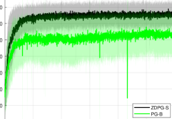
In section 5, we presented the learning curves for our algorithm implemented on a navigation problem with and without system noise. We showed that either with or without system noise, ZDPG and ZDPG-S enjoy a substantial advantage over PG with baseline (PG-B), and of course standard PG, especially without MC variance reduction, which is of importance in various practical settings. The main purpose of this section is to confirm that the advantage of ZDPG does not disappear as the noise in the system further increases; in fact, it becomes even more drastic. We show this by comparing the learning curves on our navigation example for system noise variance $\omega=0.01$ and $\omega=0.1$, for different values of Monte-Carlo variance reduction $(N)$, and policy evaluation rollout length $(T)$. In this set of simulations, we only compare ZDPG-S with PG-B, since these methods seem to be empirically superior to ZDPG and PG, respectively.

In Figure 3, the evaluation rollout length is set to $T=20$. The smoothing parameter for ZDPG-S is $\mu=0.5$ for the $\omega=0.01$ system noise case and $\mu=0.6$ for the $\omega=0.1$ system noise case. Analogously, for PG-B, we select action variance as $0.025$ for both levels of system noise as this value showed the most consistent performance throughout this line of experiments (by trial-and-error). For all simulations and for both methods, the learning rate was set to $\alpha=10^{-7}$. Figure 3 (top) shows that, indeed, ZDPG-S remains advantageous over and consistently outperforms PG-B when the system noise is increased. More interestingly, ZDPG-S shows significant advantage over PG-B in terms of noise resilience especially when there is no MC variance reduction at all (i.e. $N=1$), which, as also stated above, is a case of interest in most practical scenarios.

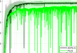
Figure 4 shows the learning curves for both methods when the evaluation length is set to $T=100$. While the performance of both ZDPG-S and PG-B is more sensitive over such a longer evaluation horizon, the plots show that ZDPG-S experiences much more stability in solving the navigation problem for both levels of system noise. In contrast, PG-B becomes significantly unstable, resulting in trajectories that either do not necessarily reach the target (see Figure 2), or reach the target after a phase of prolonged, suboptimal wandering.
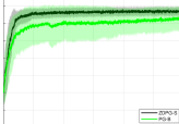
Because PG-B relies on the estimate (Q^โ€‹(s,a)โˆ’V~โ€‹(s)^๐‘„๐‘ ๐‘Ž~๐‘‰๐‘ \hat{Q}(s,a)-\tilde{V}(s)), MC variance reduction (whenever $N>1$) is essentially applied to both parts of the involved two-point difference for the results presented in Figure 3 (and analogously for the two-point gradient estimates in ZDPG). In that way, the comparison between ZDPG and PG-B is fair for every $N\geq 1$. Still, it would be interesting to compare ZDPG-S with PG-B, when in the latter a more accurate version of the corresponding true value function is employed, resembling a standard (non-stochastic) PG with baseline. To do this, we conducted the same experiment as in Figure 3 for the low system noise case ($\omega=0.01$) and with no MC reduction ($N=1$), but where only the baseline V~โ€‹(s)~๐‘‰๐‘ \tilde{V}(s) is constructed as a multiple-rollout estimate of the associated value function at state s๐‘ s (i.e., an average). We note, though, that this procedure results in a PG-B algorithm which is much more wasteful in terms of resources, whereas at the same time its comparison with ZDPG is extremely unfair, in favor of ZDPG. This resulting plots are shown in Figure 5. It very interesting to see that, even though the performance of PG-B slightly improves with the consideration of multiple-rollouts for the corresponding value function estimate, it still performs rather poorly compared with ZDPG-S, which of course demands just two system rollouts per episode.

Again, we would like to reiterate that the success of ZDPG comes from the non-heuristic use of deterministic policies, in contrast to random policies essential in log-trick-based standard (baseline) PG methods. At least with regards to our simulation setting, removing this level of randomness from the evolution of the system during training allows the agent to reach a solution quickly and consistently.