2 Department of Physics and IPAP, Yonsei University, Seoul 03722, Republic of Korea
Gravitational wave signals of dark matter freeze-out
Abstract
We study the stochastic background of gravitational waves which accompany the sudden freeze-out of dark matter triggered by a cosmological first order phase transition that endows dark matter with mass. We consider models that produce the measured dark matter relic abundance via (1) bubble filtering, and (2) inflation and reheating, and show that gravitational waves from these mechanisms are detectable at future interferometers.
1 Introduction
The identity of dark matter (DM) and its production mechanism are among the most important open questions in physics. In the weakly interacting massive particle (WIMP) paradigm, with its thermal freeze-out mechanism, the measured DM relic density requires a WIMP mass of GeV, and an electroweak-scale DM annihilation cross section. The decoupling temperature is related to the DM mass by . The vanilla version of this scenario had been challenged by the non-observation of WIMPs in DM direct detection searches. Alternative scenarios for DM production in the early universe often assume a DM sector that is out of thermal equilibrium with the standard model (SM) sector. For example, DM may be produced in the decays of a heavy particle Kolb:1998ki ; Allahverdi:2018iod . DM may also be produced by freeze-in through the feeble annihilation of particles which are thermalized with the SM bath McDonald:2001vt ; Hall:2009bx ; Chu:2013jja . However, in all of the above scenarios, the DM mass is constant during DM production.
The discovery of the 125 GeV SM-like Higgs boson at the Large Hadron Collider (LHC) Aad:2012tfa ; Chatrchyan:2012xdj consolidates spontaneous symmetry breaking as the mechanism that gives the SM particles their mass. The Higgs mechanism gives the simple relation between the fermion mass and its Yukawa coupling to the Higgs boson , where GeV is the vacuum expectation value (VEV) of the SM Higgs. A picture of the universe going through an electroweak phase transition because finite temperature effects modify its scalar potential as the universe cools down, emerges. Before the phase transition, when all the SM particles are massless, the global minimum of the scalar potential is located at . After the phase transition, the global minima of the potential shift to non-trivial values , which gives mass to the SM particles. In the SM, the electroweak phase transition is found non-perturbatively to be a smooth crossover crossover1 ; crossover2 . However, since we do not fully understand the entire structure of the scalar potential of the 125 GeV Higgs boson, and since the existence of additional scalars is a possibility, the nature of the transition is unknown.
The DM mass may be generated by a similar mechanism Hambye:2013sna ; Hambye:2018qjv ; Heurtier:2019beu ; Baker:2019ndr ; Chway:2019kft . The mass originates from its couplings to a scalar, which obtains a non-trivial VEV in the early universe, so that massless DM becomes massive during the phase transition. The scalar may or may not be the 125 GeV Higgs boson. We consider a first order phase transition (FOPT) in the early universe, with vacuum bubbles nucleated at temperature , which ends with the expanding bubbles populating the entire universe; until we discuss inflationary supercooling, we do not differentiate between the nucleation temperature and the temperature at which gravitational waves are produced. The symmetric and broken phases are located outside and inside the bubbles, respectively. The massless DM particles outside the bubbles become massive when they enter the bubbles. Only massless DM particles that carry kinetic energy larger than can penetrate the bubble walls and become massive. DM inside the bubbles abruptly decouples from the thermal bath if . The result is that the bubbles filter out a certain amount of DM and determine the DM relic abundance Baker:2019ndr ; Chway:2019kft . The massless DM outside the bubbles remains thermalized with SM radiation. It is also possible that all the massless DM particles enter the bubbles after being diluted by a period of inflation, which determines the relic abundance Hambye:2018qjv . DM particles with insufficient kinetic energy to enter the bubbles, bounce back to the symmetric phase and slow down the bubble expansion by applying pressure on the bubble walls.
The value of needed to produce the correct DM relic abundance depends on the velocity of the bubble walls . For instance, for TeV and , which satisfies . Note that DM freeze-out induced by a FOPT can easily accommodate DM masses above a PeV, which is beyond the current sensitivities of DM direct detection and LHC searches.
In this paper, we focus on gravitational wave (GW) signals of sudden DM freeze-out caused by a FOPT during which DM mass is generated. Because the power and frequency spectrum of the GW signal is model dependent, we choose two example models, Scalar Quartic Model Kehayias:2009tn ; Wang:2020jrd ; Dine:1992wr ; Adams:1993zs and Model Hambye:2018qjv ; Hambye:2013sna , to demonstrate that in parameter space regions that yield the observed DM relic abundance, a detection is possible at future GW interferometers. In the Scalar Quartic Model, the DM abundance is determined by bubble filtering, while in the Model, the DM abundance is set by inflation and reheating.
The paper is organized as follows. Bubble filtering is described in section 2, and computations of the bubble wall velocity are detailed in section 3. In section 4, we list the contributions to GW spectra from various processes. We calculate the GW signals for the two example models in section 5, and summarize in section 6.
2 Bubble filtering
During the FOPT and bubble expansion, massless (massive) DM particles are located outside (inside) the bubble, and momentum conservation must be satisfied at the bubble wall. An incident DM particle enters the bubble if it carries kinetic energy larger than its mass inside the bubble. Otherwise, the massless DM particle is reflected and stays outside the bubble. If a thermal flux of is incident on the wall, the number density of DM particles that enter the bubble is Chway:2019kft
| (1) |
where is the Lorentz boost factor of the wall in the rest frame of the plasma, is the number of spin states of the DM particle, and the DM distribution has been approximated to be Boltzmann. In the non-relativistic limit, , filtering strongly suppresses the DM number density inside the bubble as . In the relativistic limit, , the number density , so there is very little filtering and approaches the equilibrium number density outside the bubble, .
If is lower than the thermal decoupling temperature , the DM inside the bubble is already decoupled from the thermal bath and makes up the DM relic abundance, On the other hand, if , the DM filtered by the bubble wall remains in thermal equilibrium and the relic abundance is determined by standard thermal freeze-out with .111Note that even with the FOPT, is obtained by equating the Hubble expansion rate and the thermal averaged DM annihilation rate, Baker:2019ndr . We assume that the SM makes a dominant contribution to the light degrees of freedom so that with logarithmic corrections that depend on , and the DM coupling.
The DM abundance today can be calculated by dividing (at ) by the entropy density , where is the effective number of relativistic degrees of freedom associated with entropy, and normalizing to the critical density, Baker:2019ndr :
| (2) |
Using Eq. (1), this can be simplified to
| (5) |
Then, requires
| (8) |
For example, for , taking TeV and , requires
| (9) |
to give the measured DM relic abundance, .
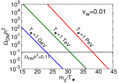
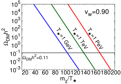
The DM relic abundances for three values of and relativistic and non-relativistic wall velocities are shown in Fig. 1. The left-panel shows that for small , if and . For (right panel), because bubble filtration is not efficient, larger values, , in the exponent of Eq. (1) are needed to suppress the DM number density. That larger requires larger can be understood by combining Eq. (1) and (2): .
3 Bubble wall velocity
We consider a fermionic or bosonic DM particle that couples to a scalar (that could be the SM Higgs or a new particle) with coupling (not to be confused with , the number of spin states). The scalar undergoes a FOPT at temperature , during which the VEV jumps from to . Nucleation starts at , and the bubbles expand and merge until the entire universe is populated with the phase. During the bubble expansion two phases coexist. Inside the bubbles , and DM gets a mass . Outside the bubbles, is massless because . Bubble filtering occurs as described in the previous section.
DM particles that are reflected by the bubble wall exert pressure on it, and slow down the bubble wall velocity, which is given by the equilibrium condition , where is the potential energy difference between the false and true vacua. The strength of the phase transition is defined in terms of the latent heat of the transition,
| (10) |
where the radiation energy density, , with the number of effectively massless degrees of freedom at temperature . For the SM, far above the electroweak scale, . Note that the derivative term in Eq. (10) is negligible for strong, supercooled transitions, as is the case for the Model.
In the ultrarelativistic limit, the pressure on the bubble wall can be obtained from the difference in the number of light degrees of freedom inside and outside the bubble Chway:2019kft ; Espinosa:2010hh ; Bodeker:2009qy :
where the ratio of the number of light degrees of freedom is
with and , the number of degrees of freedom of the bosons and fermions, respectively. If particle of the thermal plasma gains mass inside the bubble and , then most of the particles fail to penetrate the wall and instead exert pressure on it Chway:2019kft . If is fermionic DM with , then including particle and antiparticle contributions. Therefore, once is known from the scalar potential, can be obtained by solving the equation, :
| (11) |
In the limit , with , we find from Eq. (11). Eliminating from Eq. (9) yields the condition,
| (12) |
to produce the measured relic abundance for TeV. If we assume , a large and small is required.
A precise computation of the bubble wall velocity outside the ultrarelativistic regime is beyond the scope of this paper. For bubble wall velocities faster than the speed of sound in the plasma (), but not ultrarelativistic, we use the approximation Steinhardt:1981ct ,
| (13) |
For (i.e., ), the condition for is
| (14) |
The wall velocity in Eq. (13) is fixed by the Chapman-Jouguet condition for fluid expansion in chemical combustion. Since this condition is generally not fulfilled Laine:1993ey ; Espinosa:2010hh , we consider a range of velocities around the value of Eq. (13) to parameterize the uncertainty in the predicted GW signal.
4 Gravitational wave production
A FOPT generates GWs from three processes Caprini:2015zlo : i) Bubble collisions. ii) Sound waves in the plasma following bubble collisions and before the kinetic energy is dissipated by bubble expansion. iii) Magnetohydrodynamic (MHD) turbulence in the plasma after the bubble collisions. The parameters that control the signal are , , the phase transition strength , the inverse of the duration of the phase transition in units of the Hubble parameter at , all of which are model and scalar potential specific.
Our calculations of the GW spectra follow the semi-analytic treatment in Refs. Huber:2008hg ; Espinosa:2010hh ; Caprini:2015zlo . Here, we simply point out some aspects of the three contributions without regurgitating the equations used. Increasing the values of and increases the peak GW frequency, but the latter also suppresses the power of the GW signal. The power also decreases as is decreased. These properties are shared by all three GW contributions.
The GW contribution from bubble collisions can be calculated directly from the scalar field in the envelope approximation. In this approximation, an important quantity is the fraction of latent heat transformed into scalar field gradient energy, .
GWs are produced by the sound waves created during percolation. For values of not too close to the sound speed or speed of light, parametric fits to the numerically obtained GW spectrum can be found in Ref. Caprini:2015zlo . These fits include an efficiency parameter for the fraction of latent heat transformed into bulk motion of the fluid, that depends on the expansion mode of the bubble. The peak frequency of the contribution from sound waves is inversely propositional to .
The contribution from MHD turbulence arises when percolation transfers a fraction of the latent heat into turbulence in the plasma. This parameter is related to via , where represents the fraction of bulk motion that is turbulent. The value of is still under investigation, and we conservatively take Caprini:2015zlo , which makes the contribution from MHD turbulence small.
Even in the case of significant supercooling, as shown in Ref. Bodeker:2017cim , bubble walls do not runaway because of friction provided by transition radiation. In our study of the Model, we explicitly check that the vacuum contribution driving the expansion dominates the pressure difference due to transition radiation across the wall. Then, the walls carry most of the energy and the GW signal arises from bubble collisions.
5 Models
We now investigate two example models to demonstrate that abrupt DM freeze-out produces a detectable stochastic GW background.
We consider the Scalar Quartic Model and Model. Both models have a quartic term as the highest order term in their scalar potentials. However, in the former model, the effective scalar potential is composed of only one scalar field , and may be viewed as approximating a multi-field potential. There may be thermal or non-thermal contributions to the cubic term from new particles that are not heavy enough to be integrated out Wang:2020jrd . In this model, the DM candidate is unspecified. On the other hand, the Model has the SM gauge group with an extra , and the scalar potential at the Planck scale is assumed to only permit quartic terms built from the SM scalar doublet and a scalar doublet under . The absence of quadratic terms renders the model dimensionless at tree level. The quadratic terms and electroweak scale are dynamically generated Heikinheimo:2013fta ; Heikinheimo:2013xua , and the vector bosons are automatically stable and are the DM candidates Hambye:2008bq ; Cirelli:2005uq . A generalization of this model that includes mass terms at tree level has been studied in Ref. Baldes:2018emh .
5.1 Scalar Quartic Model
The effective scalar potential at finite temperature is Kehayias:2009tn ; Wang:2020jrd ; Dine:1992wr ; Adams:1993zs
| (15) |
where we have neglected non-thermal contributions to the cubic term. Many particle physics models such as the inert singlet, inert doublet, and minimal supersymmetry models, can be parametrized by the above finite-temperature effective potential. We identify with the SM Higgs and set the zero-temperature VEV to the SM value . Since is not the Higgs trilinear coupling, but the -independent coefficient of the term of the high- expansion of the Higgs effective potential, we take as a free parameter. Then the critical temperature is Wang:2020jrd
| (16) |
where
| (17) |
is the temperature when the potential barrier vanishes. The two minima are
| (18) |
There are three independent parameters , and in the above effective potential. For simplicity, we fix in following analysis.
The nucleation temperature is determined by requiring the bounce action , when the vacuum tunneling rate equals the Hubble expansion rate Kehayias:2009tn . We adopt the following analytic approximation from Ref. Adams:1993zs :
| (19) |
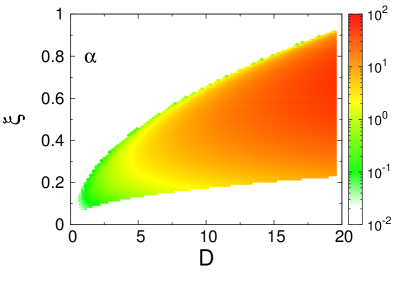
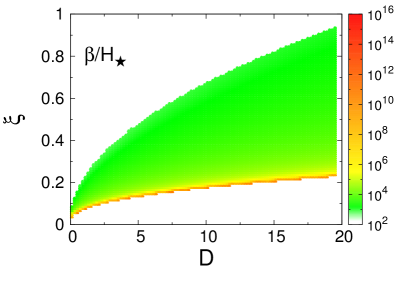
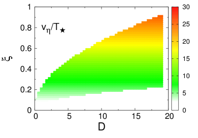
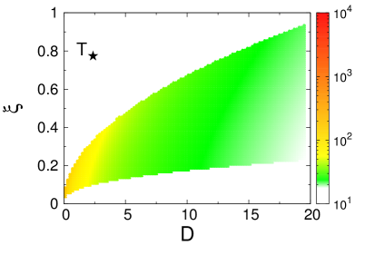
where , and , and are the results of a numerical fit. The expression is valid for which corresponds to . We choose to compute and Kehayias:2009tn . Figure 2 shows that in only narrow parameters region (for example around ), is large enough () as dictated by Eq. (14), to obtain the measured DM relic abundance for .
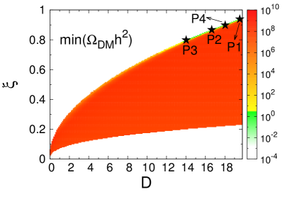
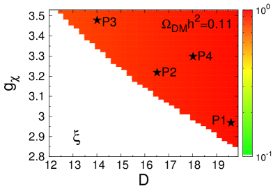
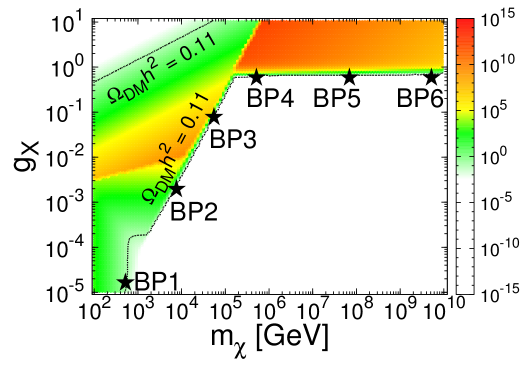
The DM relic abundance is mainly determined by bubble filtering in the Scalar Quartic Model. Because of the presence of the quadratic term at tree-level, inflationary supercooling (as for the Model) does not occur. In the left panel of Fig. 3, we show values of the relic abundance obtained by varying and with . In most of the parameter space DM is overproduced. However, in the narrow green region ; compare with the upper-left panel of Fig. 2. The values of and for which are displayed in the right panel of Fig. 3. The four benchmark points marked with stars in Fig. 3 are listed in Table 1.
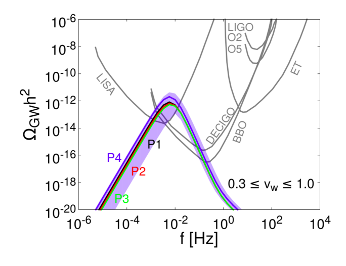
The GW spectra for the benchmark points are shown in Fig. 4. The frequencies peak around Hz because for all four points. This puts the model out of reach of LIGO and ET. LISA, BBO and DECIGO are sensitive to all four benchmark points because they have which generates a large peak signal strength, .
P1 P2 P3 P4 0.943 0.863 0.796 0.901 19.7 16.5 14.0 18.0 2.97 3.22 3.48 3.31 0.089 0.082 0.076 0.121 1116 1062 1015 1085 25.71 23.41 21.49 24.51 0.768 0.763 0.760 0.791 21.5 23.8 26.1 22.7 1642 1799 1953 1838
5.2 Model
In this dimensionless model, the SM gauge group is extended by an with gauge coupling , and a scalar , which transforms as a doublet under and is a singlet under the SM gauge group Hambye:2018qjv ; Hambye:2013sna . The scalar potential at tree level is
| (24) |
is spontaneously broken after acquires a VEV . We treat the three vector bosons of cumulatively as a single DM candidate with and mass .
In this model, as the universe cools down, the universe remains trapped in the false vacuum (i.e., ) during thermal inflation due to the thermal effects. Around this vacuum, all particles are massless. When the energy of the false vacuum exceeds the radiation energy (i.e., ), thermal inflation begins at temperature with Hubble constant , which are given by
| (25) |
During this phase, all particles undergo supercooling, because the scale factor grows exponentially and the temperature falls inversely with the scale factor. Supercooling ends at temperature with a phase transition to the true vacuum at . Supercooling ends when the temperature falls to the nucleation temperature , or earlier at the QCD phase transition temperature if :
| (26) |
where MeV.
The Coleman-Weinberg mechanism generates a true minimum at when the quartic becomes negative at a scale, Hambye:2018qjv . Assuming the true vacuum has zero energy, the energy in the false vacuum is , which implies that supercooling starts at Hambye:2018qjv
| (27) |
To compute the GW spectra we take Baldes:2018emh . To calculate , we use the bounce action,
| (30) |
which exactly reproduces the numerical result in Fig. 1 of Ref. Hambye:2018qjv . Nucleation occurs when .
After inflation ends, the universe is reheated by the transfer of vacuum energy from the scalars to the other particles. How quickly this occurs determines the reheating temperature . If the scalars decay rapidly, , and if they oscillate and transfer energy at a rate much slower than the Hubble rate before decaying, is lower, i.e.,
| (31) |
We assume that the energy transfer rate is dominated by Higgs decay, so , where the Higgs decay width, MeV.
5.2.1 Dark matter abundance
Having calculated , and , we now consider the DM relic abundance in two regimes: and , where is the decoupling temperature in the conventional freeze-out scenario. For , the DM abundance is dictated by supercooling and by sub-thermal production via scattering. Although we account for bubble filtering, its effect is negligible. On the other hand, for , the supercooled population is washed out, and the sub-thermal population reattains thermal equilibrium and produces the relic abundance as in the standard freeze-out scenario. The contour in the upper-left corner of Fig. 5 corresponds to this case.
The DM abundance resulting from inflationary supercooling is
| (32) |
where quantifies the filtering effect with in Eq. (1). However, for most of the parameter space of this model because the bubble wall velocity is close to the speed of light and . The dilution from supercooling is significant for , and can lead to DM being under-produced; this corresponds to the white region in the lower-right corner of Fig. 5. The DM density today can be calculated by rescaling from to the temperature today, 0.235 meV, and using Eq. (2).
We now consider sub-thermal DM production after supercooling. The decoupling temperature of this population is , where , and is the thermal averaged DM annihilation cross section of the process Hambye:2018qjv . The abundance of the sub-thermal population is obtained by solving the Boltzmann equation.
For , both supercooling and sub-thermal production contribute to the DM relic abundance,
| (33) |
For , the plasma thermalizes again, and the usual freeze-out mechanism yields the relic abundance,
| (34) |
The DM relic abundance is shown in Fig. 5. We mark six benchmark points along the dashed curves (which indicate ), and their values are listed in Table 2. For BP2 and BP3 sub-thermal processes dominate. Dilution by supercooling fixes the DM abundances for BP1, BP4, BP5, and BP6. The end of supercooling occurs at the nucleation temperature for BP4, BP5 and BP6, and at the QCD phase transition temperature for BP1. For the contour in the upper-left corner of Fig. 5, and the DM abundance is produced by the usual thermal freeze-out. However, we have checked that the pressure difference due to transition radiation across the wall becomes larger than the vacuum pressure driving the bubble expansion Bodeker:2017cim . Since this renders our assumption that GWs are predominately produced by bubble collisions invalid, we do not consider this part of the parameter space any further.
BP1 BP2 BP3 BP4 BP5 BP6 540 10.7 12.5 14.4 2.42 46.6 422 2082 3566 14.5 0.201 63.6 629
5.2.2 Gravitational wave signals
To calculate the GW spectra, we need the phase transition strength , inverse phase transition duration , , and . We evaluate and by following the procedure of Section 3 and replacing by in Eq. (10) to make the equation valid for vacuum transitions Caprini:2015zlo . The bounce action is used to find . We take , and rescale the peak frequency by and the amplitude by to account for a period of matter domination after the phase transition Baldes:2018emh . The values of these parameters are provided in Table 2 for the six benchmark points. The extremely large values of and are representative of ultra supercooling, for which the pressure cannot counter the vacuum energy , so that bubble expansion keeps accelerating, until the bubbles collide and produce GWs. All our benchmark points satisfy the requirement that is much larger than the pressure from transition radiation Baldes:2018emh :
| (35) |
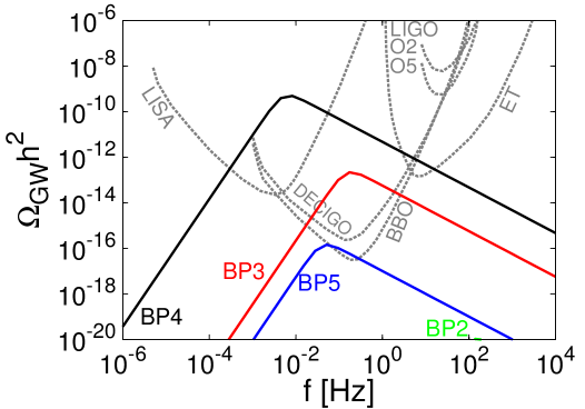
In Fig. 6, we display the GW spectra for a few benchmark points and the sensitivities of the LIGO O2 and O5 observing runs Aasi:2013wya , LISA Caprini:2015zlo ; Auclair:2019wcv , ET Hild:2010id , BBO Yagi:2011wg , and DECIGO Kawamura:2019jqt are provided for comparison. The BP1, BP2 and BP6 signals are suppressed to an unobservable level because of the large for BP1 and BP2, and small for BP6. BP3 and BP4 produce strong signals at BBO and DECIGO, and BP5 is marginally detectable at BBO. BP4 can also be detected by LISA, and marginally by ET.
6 Summary
We studied the sudden freeze-out of DM as an alternative to the continuous thermal freeze-out mechanism. A necessary ingredient for sudden freeze-out is that a FOPT generates DM mass. DM mass is generated via the coupling to a scalar particle, whose potential is responsible for a FOPT. When the scalar field acquires a non-zero VEV, DM becomes massive. The DM relic abundance may be determined by bubble filtering or by inflation and reheating. Because a FOPT triggers sudden DM freeze-out, GWs offer a signature for sudden freeze-out not available for thermal freeze-out.
To assess the viability of GWs as a signal of sudden freeze-out, we considered two example models that produce a DM abundance either by bubble-filtering (Scalar Quartic Model) or by inflation and reheating ( Model). We showed that the observed DM relic abundance can be realized in these models with detectable GW signals in future interferometers.
In the Scalar Quartic Model, the perturbativity condition, , forces the preferred parameter space to have a large and small phase transition strength, . To produce the DM relic abundance, the expanding bubbles must filter out most of the thermal DM in the symmetric phase via a large and non-relativistic bubble wall velocity. In these parameter regions the GW spectra have peak frequencies Hz, and powers large enough to be probed by LISA, DECIGO, and BBO.
In the Model, bubble filtering has a negligible effect on the DM number density, and the DM relic abundance is governed either by supercooling during thermal inflation or sub-thermal DM production. The parameter regions that give the DM relic abundance favor , which corresponds to ultra supercooling. Therefore, GWs originate from bubble collisions. Observable GW spectra have peak frequencies between about Hz to 1 Hz, and enough power to be probed by LISA, BBO, DECIGO and ET. For BP3 and BP4, the GW power is above .
Acknowledgements
We thank P. Schwaller and an anonymous referee for useful comments. D.M. is supported in part by the U.S. DOE under Grant No. de-sc0010504.
References
- (1) E. W. Kolb, D. J. H. Chung and A. Riotto, AIP Conf. Proc. 484, no. 1, 91 (1999), [hep-ph/9810361].
- (2) R. Allahverdi, K. Dutta and A. Maharana, JCAP 1810, 038 (2018), [arXiv:1808.02659 [astro-ph.CO]].
- (3) J. McDonald, Phys. Rev. Lett. 88, 091304 (2002), [hep-ph/0106249].
- (4) L. J. Hall, K. Jedamzik, J. March-Russell and S. M. West, JHEP 1003, 080 (2010), [arXiv:0911.1120 [hep-ph]].
- (5) X. Chu, Y. Mambrini, J. Quevillon and B. Zaldivar, JCAP 1401, 034 (2014), [arXiv:1306.4677 [hep-ph]].
- (6) G. Aad et al. [ATLAS Collaboration], Phys. Lett. B 716, 1 (2012), [arXiv:1207.7214 [hep-ex]].
- (7) S. Chatrchyan et al. [CMS Collaboration], Phys. Lett. B 716, 30 (2012), [arXiv:1207.7235 [hep-ex]].
- (8) K. Kajantie, M. Laine, K. Rummukainen and M. E. Shaposhnikov, Nucl. Phys. B 466, 189-258 (1996) d[arXiv:hep-lat/9510020 [hep-lat]].
- (9) K. Kajantie, M. Laine, K. Rummukainen and M. E. Shaposhnikov, Phys. Rev. Lett. 77, 2887-2890 (1996) [arXiv:hep-ph/9605288 [hep-ph]].
- (10) T. Hambye and A. Strumia, Phys. Rev. D 88, 055022 (2013), [arXiv:1306.2329 [hep-ph]].
- (11) T. Hambye, A. Strumia and D. Teresi, JHEP 1808, 188 (2018), [arXiv:1805.01473 [hep-ph]].
- (12) L. Heurtier and H. Partouche, Phys. Rev. D 101, no. 4, 043527 (2020), [arXiv:1912.02828 [hep-ph]].
- (13) M. J. Baker, J. Kopp and A. J. Long, arXiv:1912.02830 [hep-ph].
- (14) D. Chway, T. H. Jung and C. S. Shin, arXiv:1912.04238 [hep-ph].
- (15) J. Kehayias and S. Profumo, JCAP 1003, 003 (2010), [arXiv:0911.0687 [hep-ph]].
- (16) X. Wang, F. P. Huang and X. Zhang, arXiv:2003.08892 [hep-ph].
- (17) M. Dine, R. G. Leigh, P. Y. Huet, A. D. Linde and D. A. Linde, Phys. Rev. D 46, 550 (1992), [hep-ph/9203203].
- (18) F. C. Adams, Phys. Rev. D 48, 2800 (1993), [hep-ph/9302321].
- (19) J. R. Espinosa, T. Konstandin, J. M. No and G. Servant, JCAP 1006, 028 (2010), [arXiv:1004.4187 [hep-ph]].
- (20) D. Bodeker and G. D. Moore, JCAP 0905 (2009) 009, [arXiv:0903.4099 [hep-ph]].
- (21) P. J. Steinhardt, Phys. Rev. D 25, 2074 (1982).
- (22) M. Laine, Phys. Rev. D 49, 3847-3853 (1994) [arXiv:hep-ph/9309242 [hep-ph]].
- (23) C. Caprini et al., JCAP 1604, 001 (2016), [arXiv:1512.06239 [astro-ph.CO]].
- (24) S. J. Huber and T. Konstandin, JCAP 0809, 022 (2008), [arXiv:0806.1828 [hep-ph]].
- (25) D. Bodeker and G. D. Moore, JCAP 1705, 025 (2017), [arXiv:1703.08215 [hep-ph]].
- (26) M. Heikinheimo, A. Racioppi, M. Raidal, C. Spethmann and K. Tuominen, Mod. Phys. Lett. A 29, 1450077 (2014), [arXiv:1304.7006 [hep-ph]].
- (27) M. Heikinheimo, A. Racioppi, M. Raidal, C. Spethmann and K. Tuominen, Nucl. Phys. B 876, 201 (2013), [arXiv:1305.4182 [hep-ph]].
- (28) T. Hambye, JHEP 0901, 028 (2009), [arXiv:0811.0172 [hep-ph]].
- (29) M. Cirelli, N. Fornengo and A. Strumia, Nucl. Phys. B 753, 178 (2006), [hep-ph/0512090].
- (30) I. Baldes and C. Garcia-Cely, JHEP 1905, 190 (2019), [arXiv:1809.01198 [hep-ph]].
- (31) B. P. Abbott et al. [KAGRA and LIGO Scientific and VIRGO Collaborations], Living Rev. Rel. 21, no. 1, 3 (2018), [arXiv:1304.0670 [gr-qc]].
- (32) P. Auclair et al., arXiv:1909.00819 [astro-ph.CO].
- (33) S. Hild et al., Class. Quant. Grav. 28, 094013 (2011), [arXiv:1012.0908 [gr-qc]].
- (34) K. Yagi and N. Seto, Phys. Rev. D 83, 044011 (2011), [arXiv:1101.3940 [astro-ph.CO]].
- (35) S. Kawamura [DECIGO working group], PoS KMI 2019, 019 (2019).