Wide binaries are rare in open clusters

Abstract

The population statistics of binary stars are an important output of star formation models. However populations of wide binaries evolve over time due to interactions within a system’s birth environment and the unfolding of wide, hierarchical triple systems. Hence the wide binary populations observed in star forming regions or OB associations may not accurately reflect the wide binary populations that will eventually reach the field. We use Gaia DR2 data to select members of three open clusters, Alpha Per, the Pleiades and Praesepe and to flag cluster members that are likely unresolved binaries due to overluminosity or elevated astrometric noise. We then identify the resolved wide binary population in each cluster, separating it from coincident pairings of unrelated cluster members. We find that these clusters have an average wide binary fraction in the 300-3000 AU projected separation range of 2.1$\pm^{0.4}_{0.2}$% increasing to 3.0$\pm^{0.8}_{0.7}$% for primaries with masses in the 0.5–1.5 $M_{\odot}$ range. This is significantly below the observed field wide binary fraction, but shows some wide binaries survive in these dynamically highly processed environments. We compare our results with another open cluster (the Hyades) and two populations of young stars that likely originated in looser associations (Young Moving Groups and the Pisces-Eridanus stream). We find that the Hyades also has a deficit of wide binaries while the products of looser associations have wide binary fractions at or above field level.

1 Introduction

Binary systems are common, as almost half of solar-type stars (44$\pm$2%; Raghavan et al. 2010, see also more recent work by Moe & Di Stefano 2017) have one or more companions. Multiple systems have been shown to be more common around higher-mass stars with a trend to wider systems around more massive primaries (see reviews by Duchêne & Kraus 2013). Around a quarter of solar-type stars have a companion wider than 100 AU (Raghavan et al., 2010) with 4.4% of stars similar to the Sun having companions wider than 2000 AU (Tokovinin & Lépine, 2012).

Brandner & Köhler (1998) suggested that binary frequency and the separation distribution of binaries could vary significantly with star formation environment. As the field population is the combination of the outputs of countless star formation events, the field binary population is a superposition of the binary populations of all of these events (see discussion in Patience et al. 2002). Star formation is broadly categorised into clustered enviroments that are the likely progenitors of the open clusters we see in the solar neighbourhood and lower density distributed environments such as Sco-Cen or Taurus-Auriga. This latter star formation mode may be the progenitor of solar neighbourhood young moving groups.

In lower-density star forming regions such as Taurus-Auriga (Kraus et al., 2011) and Ophiuchus (Cheetham et al., 2015), wide systems are seen to exist at similar or higher frequencies to the field. Scally et al. (1999) suggested that the higher-mass Orion Nebular Cluster (ONC) had virtually no binaries wider than 1000 AU. Reipurth et al. (2007) found that the ONC had a binary fraction of 8.8$\pm$1.1% between 67.5 and 675 AU. More recently Jerabkova et al. (2019) found that the binary frequency per unit log separation was approximately 5% for binaries in the 1000-3000 AU range. However these studies of wide binarity in young populations may not translate directly to the binaries these populations will eventually contribute to the field.

Reipurth & Mikkola (2012) postulate that wide binaries are often triple systems which have evolved to one tight pair and one wide companion. This is supported by the apparently high frequency of higher-order multiplicity seen in wide systems (Law et al., 2010; Allen et al., 2012). As noted by Elliott et al. (2015), the Reipurth & Mikkola (2012) model suggests that many young wide binaries will be unstable and will not survive to field age. Thus while the population of wide binaries in star forming regions is an vital test for the output of star formation simulations, these systems may have undergone significant evolution or disruption by the time they reach field age. This means that population of wide binaries in young $<100$ Myr populations may not match the population of wide binaries from that star formation event that will eventually reach the field. Hence if one wishes to test the contribution a population of stars makes to the field wide binary population it is better to target intermediate-aged (100 Myr–1 Gyr) populations as these will suffer less future evolution due to either internal angular momentum evolution of the binary/hierarchical triple or due to external influences such as encounters with stars in the association/cluster or in the field.

We chose to study the wide binary populations of three well-studied open clusters, Alpha Per, the Pleiades and Praesepe. All three have had their memberships extensively studied using a variety of techniques. Alpha Per is a young cluster (85 Myr; Navascues et al. 2004) lying at low Galactic latitude making it the most challenging of our three clusters to study. That said there have been multiple studies of its membership (Jones & Stauffer, 1991; Rebolo et al., 1992; D. Barrado y Navascués et al., 2002; Deacon & Hambly, 2004; Lodieu et al., 2012b, 2019a). The Pleiades is the best-studied of our three clusters (Hambly et al., 1991; Deacon & Hambly, 2004; Stauffer et al., 2007; Lodieu et al., 2012a; Bouy et al., 2015; Rebull et al., 2016; Olivares et al., 2018; Lodieu et al., 2019a). It’s closeness and young age (125 Myr; Stauffer et al. 1998) have made it an ideal target to search for low-mass objects culminating in the discovery of some of the first brown dwarfs (Rebolo et al., 1995; Basri et al., 1996) and even probing down to the planet-brown dwarf boundary (Zapatero Osorio et al., 2018). Praesepe is the most distant and oldest of our clusters (790 Myr; Brandt & Huang 2015b) and as such it has proved an ideal target to study a stellar population at close to field age (Hambly et al., 1995; Hodgkin et al., 1999; Kraus & Hillenbrand, 2007; Baker et al., 2010; Boudreault et al., 2012; Rebull et al., 2017; Gao, 2019; Lodieu et al., 2019a).

Binary stars in clusters can be identified by their overluminosity (Stauffer, 1984; Rubenstein & Bailyn, 1997; Khalaj & Baumgardt, 2013; Sheikhi et al., 2016), lunar occultation (Richichi et al., 2012), radial velocity techniques (Neill Reid & Mahoney, 2000) or by direct imaging (Bouvier et al., 1997; Patience et al., 2002; Garcia et al., 2015; Hillenbrand et al., 2018). However these studies are typically limited to relatively close separations with only the direct imaging surveys going out to separations of a few hundred AU.

In this work we first identify cluster members using Gaia DR2 data (Prusti et al., 2016; Gaia Collaboration et al., 2018). We then characterise each cluster, measuring the system mass function (the mass function without a correction for unresolved binarity) and flagging objects that may be unresolved binaries. After doing this we identify pairs of objects and disentangle the population of wide binaries in each cluster from the population of coincident pairings between unrelated cluster members. We then estimate the wide binary fractions of each cluster. These wide binary fractions are then compared to those in other clusters and associations. We use this comparison to draw conclusions on the origin of the field wide binary population.

2 Cluster membership

2.1 Selecting cluster members

We implemented a probabilistic cluster member search. This method built on that undertaken by Deacon & Hambly (2004) which is based on Hambly et al. (1995) and Sanders (1971). Our method takes into account the 3D nature of the cluster while also including a statistical treatment of background contamination. Full details of the likelihood calculation are given in Appendix A.

We selected a sample of potential members from each cluster using the Gaia Archive (Prusti et al., 2016; Gaia Collaboration et al., 2018). Gaia provides exquisitely accurate astrometry with typical proper motion uncertainties of 0.1 milliarcseconds per year for $G<15$ rising to 1 milliarcsecond per year at $G=20$ as well as high-quality parallaxes. For each cluster we used the cluster centre quoted in the Simbad database. We then selected all stars in Gaia DR2 out to a radius of five degrees from the cluster centres. We list these cluster centres along with the approximate proper motions of each cluster in Table 1.

Table 1: The three open clusters we studied. The listed proper motions are the approximate Gaia proper motions of the cluster centres.

Cluster	Cluster Centre	Search radius	$\mu_{\alpha}\cos{\delta}$	$\mu_{\delta}$	$\theta$	Number of
						members
		(∘)	(mas/yr)	(mas/yr)	(∘)
Alpha Per	03 26 42.0 +48 48 00a	5	23	$-$26	48.0	801
Pleiades	03 47 00.0 +24 07 00b	5	20	$-$46	66.5	1526
Praesepe	08 40 24.0 +19 40 00b	5	$-$36	$-$13	160.0	1230
a Kharchenko et al. (2013)
b Wu et al. (2009)

For each cluster we divided the data by observed Gaia $G$-band magnitude. Objects brighter than $G=10$ mag were put into the brightest bin. We then used bins that were two magnitudes wide from $G=10$ mag to $G=18$ mag. The two faintest bins were set to be only one magnitude wide ($18<G<19$ and $19<G<20$) because astrometric errors increase faster at fainter magnitudes. We did not cut on Renormalised Unit Weighted Error (RUWE; Lindegren et al. 2018b) as we expect some binaries in the cluster to have elevated astrometric noise (see Section 3.1.1). As wide binaries often have components that are themselves binaries (Law et al., 2010; Allen et al., 2012), cutting on RUWE would bias our search against some wide binaries.

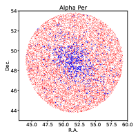
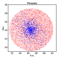
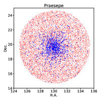
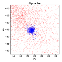
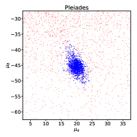
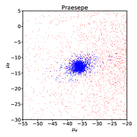
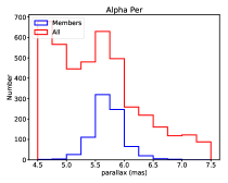
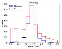
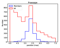
We fitted likelihoods to each magnitude bin of each cluster, allowing us to calculate membership probabilities for each star in the area around our clusters. Our fitting code did not converge for the faintest bin of Alpha Per, likely due to high background contamination caused by its low Galactic latitude. Thus our faint limit for Alpha Per is $G=19$  mag. We selected a star as a cluster member if it had a membership probability greater than 0.5. This left us with 815 Alpha Per members, 1477 Pleiades members and 1181 Praesepe members. Figure 1 shows the sky distribution plots, proper motion vector point diagrams and parallax histograms for each cluster. Our method clearly selects well-defined cluster populations. Table 4 lists all objects for which we calculate membership probabilities in each cluster.

Figure 1: Sky distribution, proper motion vector point diagrams, parallax histograms and membership probability histograms for the our three clusters. The blue points shown are objects with membership probabilities above 0.5.

2.2 Completeness and contamination

We study the completeness of our survey by using previous studies of our clusters to test how well we recover previously known objects. We expect to lose objects in a number of different ways. There will be objects which do not have a counterpart in Gaia. We will also lose objects where Gaia has only calculated a two parameter solution, making it impossible to calculate membership probabilities. There will also be objects which have proper motions and parallaxes that are so discrepant from the cluster values that they lie outside the normalisation limits for our likelihood. Additionally there are objects where the better-quality Gaia proper motions and the addition of parallax measurements reduce the object’s membership probability so that it is below 0.5.

Arenou et al. (2018) estimate that the Gaia survey completeness by comparing to the OGLE and HST data at different stellar densities. For the stellar densities found over most of they sky they recovered $>$99% of OGLE stars to fainter than $G=20$ mag. This is likely true of our clusters as they do not lie in areas of extremely high stellar density. We tested our completeness by examining the recovery fraction between our work and studies using the UKIDSS Galactic Plane Survey (Lodieu et al. 2012a in the Pleiades, Lodieu et al. 2012b in Alpha Per and Boudreault et al. 2012 in Praesepe). The Pleiades cluster has also been a target for the DANCe programme which uses a compilation of all previous observations with different surveys and telescopes to accurately measure the astrometric properties of candidate cluster members (see Bouy et al. 2015 and Olivares et al. 2018). Finally we added the Praesepe membership survey of Kraus & Hillenbrand (2007). We note that none of these surveys will themselves be 100% complete and that the recovery fractions listed here are only indicative of our true completeness.

Before beginning our completeness test we excluded any object in our comparison sample which fell outside the sky areas of our cluster search. We also excluded any object that would likely be faint enough to fall below our $G=20$ mag limit. We therefore cut on $Z<18$ mag (UKIDSS studies) and $J<16$ mag (DANCe) for Praesepe and the Pleiades and cutting on $Z<17$ mag for comparison with Lodieu et al. (2012b)’s studies of Alpha Per.

Table 2 lists the number of objects we recover from each cluster along with the number of objects lost at each particular stage. We are losing 0.0–0.4% of objects due to them lacking Gaia data and 1.1–3.9% of objects due to them having only two parameter solutions in Gaia. We found that most of the objects we miss due to low (or lack of) membership probabilities have parallax measurements that are inconsistent with cluster membership with other objects excluded due to discrepant proper motions. However, we note the Olivares et al. (2018) candidate cluster members form a distribution on a proper motion vector point diagram that is elongated along the direction of cluster motion. This is to be expected as if the cluster members have the same space velocity, then the more distant members will have slightly lower proper motions and the closer members will have higher proper motions but all will move in roughly the same direction. Indeed our work finds a higher dispersion in proper motions in the direction of cluster motion ($\sigma_{y}$).

We also compared to the recent study of Lodieu et al. (2019a). This study uses a more detailed 3D model for the cluster than our method. It also covers a much larger area and includes candidate members out to three times the tidal radii of each cluster. Our study by contrast is constrained to a smaller area around the cluster centre. Restricting ourselves to objects that fell within Lodieu et al. (2019a)’s tidal radius for each cluster and to objects bright enough to appear in our sample and which fall in our survey area, we found we recover 453/471 of Lodieu et al. (2019a)’s Alpha Per members, 1195/1225 of their Pleiades members and 696/707 of their Praesepe members. This is a 97% recovery rate across the three clusters. We also find that 814/815 of our Alpha Per members, 1473/1477 of our Pleiades members and 1147/1181 of our Praesepe members appear in Lodieu et al. (2019a)’s member list. Hence, despite our differing membership selection techniques, our membership lists for the core of each of our three clusters are almost identical.

We estimate our contamination by applying our cluster fits to control fields at the same Galactic latitude as our clusters but offset by ten degrees in Galactic longitude. Each field was three degrees in radius and the stars had the same transformation and filtering steps applied to them before having their membership probabilities analysed. These control fields should contain no true cluster members. In the Alpha Per offset field we found 32 out of 4596 stars had $p_{bin}>0.5$, 18 in the Pleiades offset field out of 5074 and 11 out of 3810 in the Praesepe offset field. Adjusting for the higher number of stars in our cluster fields (13979, 16167 and 12071 for Alpha Per, the Pleiades and Praesepe respectively) and we estimate that our cluster samples contain 97, 57 and 35 field interlopers for Alpha Per, the Pleiades and Praesepe respectively.

Table 2: Details of comparisons with previous membership studies of each cluster. We list the total number of objects which were bright enough and fell in the right sky area for us to detect ($N_{objects}$) plus the number recovered ($N_{recovered}$), how many had low membership probabilities ($N_{p_{memb}<0.5}$), how many fell outside the proper motion and parallax bounds of our membership probability calculations ($N_{nop_{memb}}$), how many had only two parameter solutions in Gaia ($N_{2parGaia}$)and how many had no Gaia counterpart ($N_{noGaia}$).

Study	Cluster	$N_{objects}$	$N_{recovered}$	Recovery	$N_{p_{memb}<0.5}$	$N_{nop_{memb}}$	$N_{2parGaia}$	$N_{noGaia}$
				percentage
Lodieu et al. (2012b)	Alpha Per	726	474	65%	148	78	23	3
Lodieu et al. (2019a)	Alpha Per	471	453	96%	18	0	0	0
Lodieu et al. (2012a)	Pleiades	1618	1346	83%	156	71	45	0
Bouy et al. (2015)	Pleiades	1947	1393	72%	436	62	52	4
Olivares et al. (2018)	Pleiades	2426	1356	56%	896	86	81	4
Lodieu et al. (2019a)	Pleiades	1225	1195	98%	29	1	0	0
Boudreault et al. (2012)	Praesepe	677	513	76%	103	37	21	3
Kraus & Hillenbrand (2007)	Praesepe	1134	914	81%	161	18	41	0
Lodieu et al. (2019a)	Praesepe	707	681	96%	26	0	0	0

2.3 Properties of cluster members

We estimated the masses for each of our potential cluster members using absolute Gaia $G$ magnitudes calculated using each star’s measured Gaia parallax. These absolute magnitudes were then converted into masses using isochrones from PARSEC stellar evolution models (Marigo et al., 2017) with the appropriate age and metallicity for each cluster. For the Pleiades we used an age of 125 Myr (Stauffer et al., 1998) and a metallicity of $[Fe/H]=-0.01$ (Netopil et al., 2016); for Praesepe 790 Myr (Brandt & Huang, 2015b) and $[Fe/H]=0.16$ (Netopil et al., 2016); and for Alpha Per 85 Myr (Navascues et al., 2004) and $[Fe/H]=0.14$ (Netopil et al., 2016). To produce a system mass function we then summed the membership probabilities of all stars in a particular mass bin weighting by the inverse of our incompleteness estimates from the previous section. We then used the scipy curvefit package to fit a log-normal function of the form

$$\xi(m)=\frac{dn}{d\log_{10}m}\propto e^{-\frac{(\log_{10}m-log_{10}m_{c})^{2}}{2\sigma^{2}}}$$ (1)

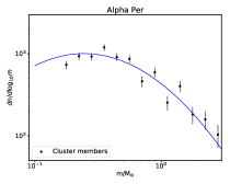
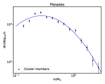
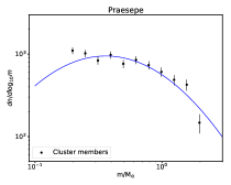
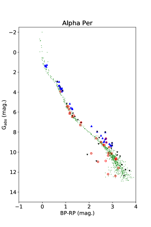
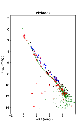
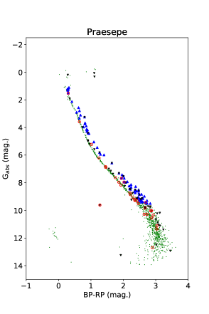
to each system mass function. We started our system mass function at the mass which was equivalent to $G=19$ mag for the Pleiades and Praesepe and $G=18$ mag for Alpha Per. This was because we found that the Gaia data became incomplete at fainter magnitudes. We found parameter values of $\log_{10}m_{c}=-0.611\pm 0.125$ ($m_{c}=0.24\,M_{\odot}$) & $\sigma=0.470\pm 0.065$ for Alpha Per, $\log_{10}m_{c}=-0.556\pm 0.038$ ($m_{c}=0.28\,M_{\odot}$) & $\sigma=0.392\pm 0.025$ for the Pleiades and $\log_{10}m_{c}=-0.442\pm 0.083$ ($m_{c}=0.36\,M_{\odot}$) & $\sigma=0.432\pm 0.063$ for Praesepe. These values are broadly similar to the previously derived values of $\log_{10}m_{c}=-0.46\pm 0.05$ & $\sigma=0.45\pm 0.02$ for the Alpha Per (Lodieu et al., 2012b), $\log_{10}m_{c}=-0.62\pm 0.02$ & $\sigma=0.44\pm 0.01$ for the Pleiades (Lodieu et al., 2012a) and $\log_{10}m_{c}=-0.60$ & $\sigma=0.55$ for the field system mass function of Chabrier (2005). Figure 2 shows our mass function for each cluster and Table 3 gives the values for the individual system mass function bins for each cluster.

Figure 2: System mass functions for the our three clusters. The blue lines show log-normal fits to each mass function. Points covered by red crosses were excluded from the system mass function fits.

Table 3: The individual bin values for our calculated system mass functions for each cluster.

Alpha Per		Pleiades		Praesepe
mass range	$\frac{dn}{d\log_{10}m}$	mass range	$\frac{dn}{d\log_{10}m}$	mass range	$\frac{dn}{d\log_{10}m}$
(M⊙)		(M⊙)		(M⊙)
…		0.120–0.151	914	…
0.157–0.198	735	0.151–0.190	1252	…
0.198–0.249	937	0.190–0.239	1949	0.175–0.220	1101
0.249–0.313	925	0.239–0.301	2098	0.220–0.277	1020
0.313–0.394	1196	0.301–0.379	1565	0.277–0.349	836
0.394–0.496	913	0.379–0.478	1484	0.349–0.440	979
0.496–0.625	867	0.478–0.601	1183	0.440–0.553	762
0.625–0.787	462	0.601–0.757	1036	0.553–0.697	849
0.787–0.991	593	0.757–0.953	747	0.697–0.877	735
0.991–1.247	254	0.953–1.200	694	0.877–1.104	608
1.247–1.570	403	1.200–1.511	376	1.104–1.390	487
1.570–1.977	182	1.511–1.902	243	1.390–1.750	425
1.977–2.488	159	1.902–2.394	109	1.750–2.050	147
2.488–3.133	104	2.394–3.014	72	…
3.133–3.944	30	3.014–3.794	48	…
3.944–4.965	58	…		…

Table 4: Membership probabilities for objects with $p_{memb}>0.5$ for each cluster. The positions, proper motions and parallaxes are taken from Gaia DR2.

Gaia source ID	R.A.	Dec.	$\mu_{\alpha}\cos{\delta}$	$\mu_{\delta}$	$\varpi$	$G$	mass	$p_{memb}$
	(J2000 Ep=2015.5)		(mas/yr)	(mas/yr)	(mas)	(mag)	(M⊙)
Alpha Per
439440029866690944	02 57 05.23	+49 39 29.3	25.7$\pm$0.3	-24.6$\pm$0.2	5.6$\pm$0.1	17.3	0.27	0.97
439191437159059968	02 57 54.15	+48 52 43.1	24.9$\pm$0.1	-22.0$\pm$0.1	5.5$\pm$0.1	8.7	1.73	0.90
434488516689743232	02 59 24.83	+47 07 49.8	23.9$\pm$0.3	-22.3$\pm$0.2	5.7$\pm$0.1	17.2	0.28	0.89
437601096669764736	02 59 35.66	+48 12 19.0	24.6$\pm$0.2	-22.1$\pm$0.2	5.5$\pm$0.1	16.4	0.4	0.70
439161986569729280	03 00 50.16	+49 01 59.4	25.2$\pm$0.6	-22.7$\pm$0.5	5.4$\pm$0.3	18.7	0.17	0.54

3 Binarity

3.1 Flagging potential unresolved pairs

The components of wide binary systems can themselves be close binaries. Such higher order multiples are common and the components of wide binaries might even be more likely to be close pairs than isolated field stars (Allen et al., 2012; Law et al., 2010). The dynamical evolution of higher order multiplies has been suggested as a formation mechanism for wide binaries (Reipurth & Mikkola, 2012). We identify possible higher-order multiples via two features: excess astrometric noise in Gaia, and overluminosity.

3.1.1 Stars with noisy astrometric solutions

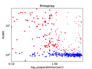
Binary companions introduce additional astrometric noise via several effects. When unresolved they can add shifts in the binary photocentre due to astrometric motion or due to photometric variability of one or both components. When resolved they can add additional astrometric datapoints that can confuse astrometric solution calculations. Finally, when they are partially resolved, PSF mismatch with the single-star PSF model results in higher scatter in the astrometric measurements. Gaia DR2 encapsulates the excess astrometric noise in the form of the Renormalised Weighted Error (RUWE; Lindegren et al. 2018a, b) which is similar to the the square root of the reduced $\chi^{2}$ statistic. RUWE measures the excess astrometric noise, accounting for the increase in excess noise in fainter objects and objects with extreme colours. To test how this excess noise statistic is elevated by close binarity we followed a similar approach to Rizzuto et al. (2018). We took close, directly imaged binaries (with separations within 1 arcsecond) from Kraus et al. (2016) and binaries found to be unresolved in Gaia from Ziegler et al. (2018) and Lamman et al. (2020). This sample in this latter work is a compilation of directly imaged binaries from Law et al. (2014), Baranec et al. (2016) and Ziegler et al. (2017) and counts binaries as resolved in Gaia if the secondary has a Gaia DR2 entry of its own. We follow Rizzuto et al. (2018) in using the ROBO-AO LP600 magnitude ratio quoted in Ziegler et al. (2018) as the Gaia magnitude difference (as the LP600 filter is similar to the Gaia $G$-band filter). We then use a PARSEC (Marigo et al., 2017) 2 Gyr isochrone to convert the Kraus et al. (2016) $K$-band magnitude difference to Gaia $G$-band magnitude difference.

Figure 3 shows that binaries closer than one arcsecond with magnitude differences less than four magnitudes have elevated RUWE values. We chose 1.4 as the limit for elevated RUWE as it was used as the limit in Lindegren et al. (2018b). Even at projected separations of $\rho\sim 0.1$″, we find that RUWE is elevated for binaries with magnitude differences less than three magnitudes. This complements the high recovery fraction in Gaia for binaries wider than one arcsecond (Ziegler et al., 2018). We flag objects with RUWE$>$1.4 and with no detected binary companion within one arcsecond as possible unresolved binaries or unresolved components of wide binaries.

Figure 3: A plot showing how the Renormalised Unit Weighted Error (Lindegren et al., 2018b) statistic in Gaia DR2 that measures excess astrometric noise as a function of binary separation and magnitude difference. The upward-pointing triangles are binaries from Kraus et al. (2016), the downward-pointing triangles are binaries from Ziegler et al. (2018) which are not resolved in Gaia and the small circles are binaries from Ziegler et al. (2018) resolved in Gaia. Red points are components or unresolved systems with RUWE$>$1.4.

3.1.2 Overluminous stars

To identify stars which may be overluminous due to binarity we used a simple isochrone fitting process. We use the previously mentioned PARSEC stellar evolution models (Marigo et al., 2017) to determine a star’s absolute $G$ magnitude based on its Gaia $BP-RP$ colour. However we found that the isochrones did not match the data well, especially for lower-mass cluster members. To remedy this we estimated the median offset in absolute $G$-band magnitude between estimates from $BP-RP$ colours & the PARSEC models and the values derived from Gaia parallaxes and apparent $G$ magnitude. We restricted ourselves to the brighter stars in each cluster where the isochrone still matched the observed colours and magnitudes reasonably well ($1<G_{abs}<12$ mag. for Alpha Per and the Pleiades, $1<G_{abs}<9.5$ mag. for Praesepe) but with small offsets. We found that using colours plus the PARSEC model made stars in Alpha Per and the Pleiades too faint (by 0.119 and 0.061 magnitudes respectively), while stars in Praesepe were marginally too bright (0.038 mag.). These offsets were then used to correct our estimated magnitudes based on $BP-RP$ colour. We then estimated the approximate scatter of the main sequence by calculating the median absolute deviation between the calculated Gaia $G$-band absolute magnitudes and those estimated from colours (after removing the previously mentioned offset) for objects that lay below the cluster isochrone. This approach allows us to estimate the scatter on the cluster star’s CMD distribution without being affected by overluminous binaries. We used 1.48 times these median absolute deviations as a robust estimate of the one sigma scatter (Maronna et al., 2006). These values were 0.151 mag. for Alpha Per, 0.162 mag. for the Pleiades and 0.092 mag. for Praesepe. Any star that had a calculated Gaia $G$-band absolute magnitude which was brighter than the estimated absolute $G$-band from colour by more than three times the scatter for the appropriate cluster was flagged as a possible overluminous binary. These are shown in Figure 7. When calculating the offsets and scatters we limited ourselves to $1<G_{abs}<9.5$ mag. in all clusters. However we found that using these calculated values we were able to reliably flag overluminous objects in Alpha Per and the Pleiades with $1<G_{abs}<12$ mag. while in Praesepe we were still limited to $1<G_{abs}<9.5$ mag. It is clear that we select stars that appear overluminous but that we miss a small number of clearly overluminous stars, especially in the $G_{abs}$=5-8 mag. range. This is likely due to to the fact that the offset between the absolute magnitudes estimated from the $BP-RP$ colours and the absolute magnitudes calculated from observed magnitude and parallax varies over the CMD.

3.2 Identifying comoving pairs

We searched the Gaia database for comoving companions to objects in our sample with separations up to 300 arcseconds. In works such as Deacon et al. (2014), wide binaries are identified by their common proper motion. Studying wide binaries in clusters using Gaia changes this strategy in two ways. Firstly all members of an open cluster are moving through space together. This means that there is a large population of other cluster members which are not binary companions to any particular star in that cluster but which will have common proper motion when paired with it. Secondly Gaia’s proper motions are so accurate that orbital motion outside the measurement errors of the proper motions must be taken into account. A $\sim$1000AU companion to a solar mass star will likely have an orbital velocity of $\sim$1 km/s. At the distance of our clusters this equates to a tangential motion of $\sim$1 mas/yr, significantly larger than the proper motion measurement errors. We perform a conservative cut on our data by adapting the astrometric difference defined by Deacon et al. (2017). This is the quadrature sum of the number of standard deviations that each pair of measurements for the proposed binary differ by. Including our orbital velocity term it is defined so that,

$$n_{\sigma}^{2}=\frac{(\mu_{\alpha 1}-\mu_{\alpha 2})^{2}}{(\sigma_{\mu\alpha 1}^{2}+\sigma_{\mu\alpha 2}^{2}+\mu_{orb,\alpha}^{2})}+\frac{(\mu_{\delta 1}-\mu_{\delta 2})^{2}}{(\sigma_{\mu\delta 1}^{2}+\sigma_{\mu\delta 2}^{2}+\mu_{orb,\delta}^{2}))}+\frac{(\pi_{1}-\pi_{2})^{2}}{(\sigma_{\pi 1}^{2}+\sigma_{\pi 2}^{2})}$$ (2)

Such that $\mu_{orb,\alpha}$ and $\mu_{orb,\delta}$ are set to be the one dimensional mean projections of the orbital velocity difference of each pair of stars separated by 1000 AU and situated at the mean distance of each cluster. We ignored covariance terms between proper motion and parallax.

$$\mu_{orb,\alpha}= \mu_{orb,\delta} =29.8km\,s^{-1}\times\left(\frac{1000.0}{4.74d_{cluster}(pc)}\right)$$

$$\left(\frac{1}{\sqrt{3}}\right)\left(\sqrt{\frac{(M_{1}+M_{2})}{\rho(AU)}}\right)$$

Where these proper motions are expressed in milliarcseconds per year. The first factor in the above equation converts from m/s to mas/yr at the distance of the cluster, the second factor accounts for the motion being split between three dimensions and the third factor is the total combined orbital velocity of the two stars. For both components of any potential binary, we use masses estimated from cluster isochrones. We select only pairs with $n_{\sigma}<5$.

3.3 Defining the wide binary population

Our sample of pairs will consist of a mix of true wide binaries and coincident pairings between unrelated cluster members, ignoring the presence of non-members in our sample because they are a negligible fraction of the total (see Section 2.2). We considered two populations of objects, field stars and cluster members. We then fitted likelihood distributions for both the cluster and field populations as a function of proper motion and parallax. The probability of cluster membership was then calculated for each star using these likelihood distributions. We take a similar approach where our pairs could be drawn from two different populations, true binaries and coincident pairings between cluster members. As we make use of the cluster density profile our logic is similar to that set out in Hambly et al. (1995). The full outline of the mathematical model for our likelihood is given in Appendix B. We use a likelihood that takes the form,

$$\phi= f_{comp}\phi_{comp}+(1-f_{comp})\phi_{coincident}$$ (3)

$$\phi_{comp}= \frac{e^{-r/r_{0}}}{2\pi r_{0}^{2}(1-e^{(-r_{max}/r_{0})}(1+r_{max}/r_{0}))}\frac{1}{x\log(\frac{x_{max}}{x_{min}})}$$

$$\phi_{coincident}= \frac{e^{-2r/r_{0}}c_{coincident,m_{2}}\xi(m_{2})}{2\pi(2r_{0})^{2}(1-e^{(-2r/r_{0})}(1+2r_{max}/r_{0}))}$$

$$\frac{2x}{(x_{max}^{2}-x_{min}^{2})}\normalsize$$

Where $r$ is the distance of the binary from the cluster centre, $m_{1}$ and $m_{2}$ are the masses of the primary and secondary component and $x$ is the separation of the binary on the sky in arcseconds. For the system mass function $\xi(m_{2})$ of each cluster we use the log-normal system mass functions we previously fitted for each cluster and use the perviously estimated masses for each star.

For the characteristic radii of the clusters $r_{0}$ we derive values using the distribution of stars in our membership selection and cluster centres taken from the Simbad database. We fitted exponential distribution to histograms of $r$ the distance from the cluster centre for each of our three clusters. We derived values of $r_{0}$ of 53.03 arcminutes for the Pleiades, 43.27 arcminutes for Praesepe and 62.77 arcminutes for Alpha Per.

For each cluster we maximised the likelihood as a function of $f_{comp}$. We did this by differentiating the log-likelihood such that,

$$\sum_{i}\frac{\partial\log\phi_{i}}{\partial f_{comp}}=0$$ (4)

Summing over all $i$ pairs in our sample. This gives us,

$$\sum_{i}\frac{1}{\phi_{i}}(\phi_{comp,i}-\phi_{coincident,i})=0$$ (5)

We solved the above equation using a simple bisection algorithm yielding values of $f_{comp}$ of 0.076 for the Pleiades, 0.036 for Praesepe and 0.075 for Alpha Per. Note that $f_{comp}$ the fraction of pairs that we believe to be real binaries and is not the same as $f_{bin}$ the actual binary fraction.

We were then able to estimate the probability that any particular pair is a binary using the equation,

$$p_{i}=\frac{\phi_{comp}(r_{i},x_{i},m_{1,i},m_{2,i})}{\phi(r_{i},x_{i},m_{1,i},m_{2,i})}$$ (6)

4 Results

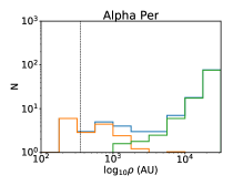
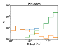
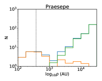
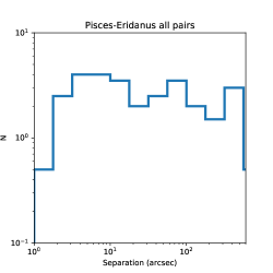
The separation histograms for our dataset are shown in Figure 6. In each we see a log-flat distribution of true binaries that is eventually swamped by coincident pairings at separations of around 3000 AU. There may be a population of true binaries at even wider separations, but the number of coincident pairs makes it hard to draw conclusions beyond  3000AU. We find 20 binaries with $p_{bin}>0.5$ in Alpha Per, 47 in the Pleiades and 28 in Praesepe. These are listed in Table 6. One of our probable pairings include a previously unknown companion to Asterope, one of the naked-eye members of the Pleiades. We note that we have a handful of very wide binaries ($>$5000 AU). These are found in the outskirts of each cluster where the density of cluster members, and hence the probability of chance alignment, is lower.

4.1 Completeness

To estimate our completeness we use the work of Hillenbrand et al. (2018) as a comparison survey. This work searched for companions to Pleiades and Praesepe members using adaptive optics. While most of their companions were at projected separations of less than an arcsecond and undetected by us, we recovered two of the four companions to stars that were in both our member selections and Hillenbrand et al. (2018)’s sample which had separations of 1.0–1.5 arcseconds, two of the three with 1.5–2.0 arcsecond separations and all three of the companions wider than that. Some of the Hillenbrand et al. (2018) targets did not appear in our sample as they fell outside our sky search area for each cluster, had no astrometric solution in Gaia or were not selected as members by our algorithm. For companions from Hillenbrand et al. (2018) that are wider than two arcseconds we do not recover four Pleiades systems. Both components in all of these systems are excluded as Pleiades members due to their parallaxes with three (s5035799, HII 659 and s5197248) having proper motions that lie outside our cluster distribution. Only DH 800 is listed as having a membership probability greater than 0.01 for either component. Only one of the components of these four binaries (the secondary of HII 659) is listed as having an elevated Renormalised Weighted Error (RUWE; Lindegren et al. 2018a, b) indicating that it is not poor-quality astrometric solutions driven by confusion that are causing these binaries to be ruled out. Indeed the primary of HII 659 also has a parallax that is discrepant with Pleiades membership ($\varpi=5.92\pm 0.05$ mas for the primary versus $\varpi=5.48\pm 0.34$ mas for the secondary). We also recover all five binaries wider than two arcseconds in Bouvier et al. (1997).

To test if missing the four wider Pleiades systems from Hillenbrand et al. (2018) is significant we extracted the SuperCOSMOS (Hambly et al., 2001) proper motions for these systems. SuperCOSMOS uses plate data with a much lower resolution and longer time baseline than Gaia. We therefore would expect binarity to affect the astrometric solutions differently from the way it affects Gaia data. We found that three of the objects (s5035799, HII 659 and s5197248) had proper motions that lay outside the proper motion distribution of Pleiades members found by Deacon & Hambly (2004) while obviously DH 800 was selected as a Pleiades member. This suggests that the absence of three wide Pleiades binaries from Hillenbrand et al. (2018) is likely due to those binaries being field interlopers or objects in the kinematic outskirts of the cluster which we exclude from our Pleiades member sample rather than any bias we have against selecting wide binary components as cluster members. The additional proper motion information of Gaia only serves to further refine the input member list that was available to Hillenbrand et al. (2018), it does not call the existence of any of their binaries into question.

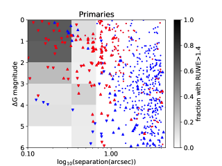
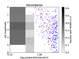
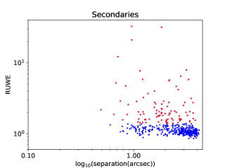
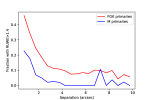
It is possible to further test if we are losing true binaries which have components that are missing from our cluster membership lists due to poor-quality astrometric solutions. To test this we examined all pairs of objects with separations up to ten arcseconds in the area around all three clusters. We chose to examine the secondary (i.e. fainter) components as these will be more likely to be affected by scattered light from a bright companion. Firstly we estimated the fraction of pairs as a function of separation that have noisy ($RUWE>1.4$) astrometric solutions for their secondary components (see the left-hand panel of Figure 4). This shows that for separations below two arcseconds there is a large fraction of objects with raised RUWE values. However beyond around three arcseconds this fraction reverts to the background level.

Figure 4: Testing the incompleteness of our survey as a function of binary separation. Here we estimate the fraction of companions to objects in the vicinity of all three clusters that have noisy astrometric solutions.

To further test our completeness we examine the work of Ziegler et al. (2018). They identified Gaia detections for components of directly imaged binaries (taken from Law et al. 2014, Baranec et al. 2016 and Ziegler et al. 2017). Their results show that almost all binaries wider than $\sim 2$ arcseconds and with magnitude differences less than 5 magnitudes have both components detected. Their sample contains few sources wider than 4 arcseconds. Arenou et al. (2018) use stars from the Washington Double Star catalogue (Mason et al., 2001) to show that binaries wider than around 4 arcseconds are complete in Gaia (their Figure 8). Hence we assume that we are complete to our faint limits for binaries wider than four arcseconds.

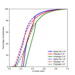
Our binary search will of course be constrained by the magnitude limit of our Gaia study. To quantify how complete we are, we estimated the binary mass ratios we could reach for each of our cluster members in each cluster (treating each as a possible primary star). We first estimated the mass of a star five magnitudes fainter than each possible primary using the PARSEC models for each cluster. This gives us a potential limiting mass for a potential companion in the 2–4 arcsecond range. If this mass was less than our lower mass limit for the cluster the star is a member of, then we used the cluster limiting mass as our limiting mass. We then divided this limiting mass by the mass of the potential primary to estimate the mass ratio above which we would be complete. We then assumed a completeness function that is zero below this mass ratio and 100% above it. Then we repeated this process for all stars in the cluster, summing the completeness functions and dividing by the number of cluster members in our sample then gives us the completeness between two and four arcseconds. These functions are shown in Figure 5. We also estimated the completeness for systems wider than four arcseconds by using the same process but only setting the limiting companion mass for each star to the lower limiting mass for the appropriate cluster. These completeness limits are also shown in Figure 5. If we assume a flat mass ratio distribution we can estimate the completeness of our sample for each cluster in each companion separation range by taking the mean of our completeness functions. Hence we find completenesses of 64% (2”–4”) & 71% ($>4"$) for Alpha Per, 64% (2”–4”) & 70% ($>4"$) for the Pleiades and 57% (2”–4”) & 63% ($>4"$) for Praesepe. It is likely that our completeness is higher than the quoted percentages. Our main source of incompleteness is undetected faint companions. Our faint limits for companions to these higher mass stars go to lower mass ratios than for companions to lower mass. These higher mass stars will be more likely to host binaries. Therefore we are likely to be more complete than our calculations around the stars most likely to host binaries. Additionally M dwarf primaries are more likely to host high mass ratio companions (Duchêne & Kraus, 2013). This means that the objects we are the least sensitive to, low mass ratio companions to low mass stars, are rare.

Figure 5: Completeness as a function of mass ratio for our three clusters both for companions in the 2–4 arcsecond range and in the $>$4 arcsecond range.

4.2 Estimating the binary fraction

We can estimate the binary fraction between 300 AU and 3000 AU for all three of our clusters. To do this we sum the binary probabilities for all pairs in this projected separation range. We then divide this by the total number of members of each cluster in our sample. Our calculation only includes binaries wider than two arcseconds in this as we are likely substantially incomplete for binaries closer than this. We then correct our calculated binary fractions by dividing by factors of $\log_{10}3000-\log_{10}2d_{cluster}$. This assumes a flat distribution in log-separation (i.e. Opik’s law Opik 1924) which broadly agrees with observations that show the separation distribution in this region is either flat (Kraus et al., 2011) or gradually declining (Raghavan et al., 2010; Tokovinin & Lépine, 2012). This takes into account the fact that cutting at separations of two arcseconds means we are incomplete for projected separations closer than $2d_{cluster}$. We also account for incompleteness for lower mass companions using the completeness estimates from Section 4.1. As we are dealing with small number statistics for our binaries we determine one sigma confidence limits using the relations of Gehrels (1986). This gives a better representation the uncertainties based on a small number of detections and leads to different upper and lower uncertainty bounds.

The calculated binary fractions in the 300–3000 AU projected separation range for stars in our three clusters are $f_{bin}=2.0\pm^{0.9}_{0.6}$% for Alpha Per, $f_{bin}=1.9\pm^{0.6}_{0.4}$% for the Pleiades and $f_{bin}=2.8\pm^{0.7}_{0.6}$% for Praesepe. The binary fractions are consistent within uncertainties. Table 5 shows the binary fractions for each cluster. We also calculate fractions for primary stars with mass estimates in the 0.5–1.5 $M_{\odot}$ range (roughly corresponding to FGK stars) and in the $<0.5$ $M_{\odot}$ range (roughly corresponding to M dwarfs). We note that the lower mass bin in each cluster has a lower binary fraction than the FGK star bin. Combining all the clusters together, the difference between the FGK and M dwarf fractions is 2.2 $\sigma$. This is consistent with previous work in young cluster (Kraus & Hillenbrand, 2009) and the field (Dhital et al., 2010) that shows that M dwarfs are less likely to be the host stars from wide binary systems than FGK stars.

Table 5: The binary fractions for different types of stars in our clusters. We use uncertainty estimates calculated with the relations of Gehrels (1986) as these are more appropriate for small number statistics. In each case we estimate the binary fraction divided by the log separation range covered $\frac{df_{bin}}{d\log_{10}x}$. Our two subranges cover approximately FGK dwarfs ($0.5<M/M_{\odot}<1.5$) and M dwarfs ($M<0.5M_{\odot}$)

	$\sum p_{bin}$	$N_{stars}$	Completeness	$d\log_{10}r$	$\frac{df_{bin}}{d\log_{10}x}$
Alpha Per
All dwarfs	11.0	815	64%	0.932	2.2$\pm^{0.9}_{0.7}$%
FGK dwarfs	8.5	250	72%	0.932	5.1$\pm^{2.4}_{1.7}$%
M dwarfs	2.4	506	53%	0.932	1.0$\pm^{1.1}_{0.6}$%
Pleiades
All dwarfs	21.7	1477	68%	1.00	2.2$\pm^{0.6}_{0.5}$%
FGK dwarfs	7.0	388	80%	1.00	2.3$\pm^{1.2}_{0.8}$%
M dwarfs	9.2	1010	59%	1.00	1.5$\pm^{0.7}_{0.5}$%
Praesepe
All dwarfs	11.8	1181	55%	0.904	2.0$\pm^{0.8}_{0.6}$%
FGK dwarfs	5.3	320	72%	0.904	2.5$\pm^{1.2}_{1.1}$%
M dwarfs	5.3	754	49%	0.904	1.6$\pm^{1.0}_{0.7}$%
All clusters combined
All dwarfs					2.1$\pm^{0.4}_{0.2}$%
FGK dwarfs					3.0$\pm^{0.8}_{0.7}$%
M dwarfs					1.4$\pm^{0.4}_{0.3}$%

Figure 6: Separation histograms for our three clusters. The blue line shows the total number of objects at each separation. The orange line shows the sum of the binary probabilities in each separation bin. The green line is the blue line minus the red line and shows the expected population of chance alignments. There is clearly an excess of pairs above the number of chance alignments below separations of around 2000AU

Table 6: A list of our probable wide binaries in Alpha Per, the Pleiades and Praesepe. All astrometry and photometry is from Gaia DR2.

Gaia ID	Position	$\mu_{\alpha}\cos{\delta}$	$\mu_{\delta}$	$\pi$	$G$	Projected		$p_{bin}$	Other name
						Separation
	(Eq.=J2000 Ep.=2015.5)	(mas/yr)	(mas/yr)	(mas)	(mag)	(”)	(AU)
Alpha Per
437596389381227648	02 58 22.98 +48 04 28.8	10.3$\pm$0.2	$-16.5\pm 0.2$	4.5$\pm$0.1	17.3	0.9	186	1.00
437596389384924544	02 58 22.99 +48 04 27.9	20.6$\pm$1.1	$-18.3\pm$0.5	4.9$\pm$0.4	18.9
439718962223158016	03 07 58.13 +50 24 35.8	24.1$\pm$0.1	$-$12.1$\pm$0.1	5.5$\pm$0.1	15.3	4.8	869	0.94	UGCS J030758.10+502436.0
439718962223158272	03 07 57.63 +50 24 36.1	24.0$\pm$0.1	$-$23.6$\pm$0.1	5.5$\pm$0.1	15.6				UGCS J030757.60+502436.3
436345969787424256	13 48.54 +48 59 11.1	23.8$\pm$0.1	$-23.8\pm 0.1$	5.4$\pm$0.1	12.0	2.6	489	0.98	TYC 3319-557-1
436345969787424896	13 48.73 +48 59 09.3	22.6$\pm$0.1	$-21.8\pm$0.1	5.4$\pm$0.1	13.7
436441176331772928	03 17 04.40 +49 20 14.6	23.6$\pm$0.1	$-$25.3$\pm$0.1	5.6$\pm$0.1	12.3	6.5	1165	0.93
436441176324119680	03 17 03.80 +49 20 11.7	21.5$\pm$0.1	$-$25.5$\pm$0.1	5.6$\pm$0.1	12.6
435680765247601536	03 17 42.13 +49 01 46.2	23.3$\pm$0.1	$-$24.3$\pm$0.1	5.6$\pm$0.1	11.7	1.5	274	0.98	AP121
435680765251589632	03 17 42.21 +49 01 44.8	22.5$\pm$0.5	$-$28.1$\pm$0.5	5.5$\pm$0.2	16.1
435184610626097408	03 18 01.20 +47 00 07.6	23.5$\pm$0.1	$-$24.3$\pm$0.1	5.8$\pm$0.1	15.2	1.7	295	0.99	DH 83
435184610626097536	03 18 01.29 +47 00 06.1	23.5$\pm$0.1	$-$25.1$\pm$0.1	5.8$\pm$0.1	15.4
242294983663641088	03 20 15.30 +45 00 10.0	19.9$\pm$0.3	$-21.2\pm$0.2	4.3$\pm$0.13	17.7	1.1	236	1.00
242294983667977472	03 20 15.25 +45 00 11.0	19.9$\pm$0.4	$-21.1\pm 0.3$	4.67$\pm$0.2	18.4
441640668031763584	03 22 32.80 +49 11 16.29	22.7$\pm$0.1	$-$26.0$\pm$0.1	5.7$\pm$0.1	16.4	2.9	484	0.96
441640668027534720	03 22 32.52 +49 11 15.49	23.2$\pm$0.3	$-$26.1$\pm$0.2	6.0$\pm$0.1	17.7				AP143
441716774852013568	03 22 40.95 +49 40 40.94	23.9$\pm$0.1	$-$25.7$\pm$0.1	5.8$\pm$0.1	12.6	4.6	783	0.87	AP107
441716774852012032	03 22 41.08 +49 40 45.32	24.3$\pm$0.2	$-$25.7$\pm$0.2	5.8$\pm$0.1	16.5
242736712463377280	03 22 55.54 +46 06 57.4	25.9$\pm$0.1	$-27.4\pm 0.1$	6.2$\pm$0.1	12.2	3.9	623	0.87	UCAC4 681-020405
242736712461022976	03 22 55.73 +46 06 54.1	25.8$\pm$0.2	$-27.1\pm 0.2$	6.2$\pm$0.1	17.0				UGCS J032255.70+460654.2
442705648117153792	03 23 20.34 +51 19 06.1	22.7$\pm$0.1	$-$23.3$\pm$0.1	5.4$\pm$0.1	13.4	1.1	205	1.00
442705648121901696	03 23 20.31 +51 19 07.2	21.5$\pm$0.1	$-$23.7$\pm$0.1	5.4$\pm$0.1	13.6
243108622271431424	03 26 22.67 +47 16 09.0	23.0$\pm$0.1	$-$25.3$\pm$0.1	5.7$\pm$0.1	11.7	7.1	1243	0.58	V627 Per AP 156 RSCVn
243108617973878272	03 26 21.98 +47 16 09.7	23.4$\pm$0.8	$-$26.1$\pm$0.4	5.9$\pm$0.3	18.5
442671563260694016	03 26 35.97 +51 22 32.5	21.1$\pm$0.1	$-$24.0$\pm$0.1	5.4$\pm$0.1	15.0	2.9	546	0.93	UGCS J032635.95+512232.6
442671563256206336	03 26 35.96 +51 22 29.6	20.5$\pm$0.7	$-$25.0$\pm$0.5	5.6$\pm$0.4	18.5
441405922299247616	03 26 50.15 +48 47 31.6	22.1$\pm$0.1	$-$26.5$\pm$0.1	5.6$\pm$0.1	10.2	4.5	813	0.83	AP51
441405922299247488	03 26 49.91 +48 47 35.4	22.3$\pm$0.2	$-$26.4$\pm$0.1	5.8$\pm$0.1	16.3
441596172170885888	03 27 50.11 +49 54 18.6	24.0$\pm$0.1	$-$26.2$\pm$0.1	5.9$\pm$0.1	15.4	14.9	2542	0.52	UGCS J032750.07+495418.9
441596172170886912	03 27 48.58 +49 54 17.9	24.2$\pm$0.2	$-$26.2$\pm$0.1	6.1$\pm$0.1	16.2				APX 155D
249111577803259264	03 28 21.96 +47 36 05.6	23.3$\pm$0.2	$-$26.6$\pm$0.1	5.8$\pm$0.1	15.7	1.1	191	1.00
249111577799138816	03 28 21.91 +47 36 06.6	24.3$\pm$0.2	$-$24.5$\pm$0.2	6.0$\pm$0.1	16.2				DH 184
249265062754562048	03 31 16.13 +48 25 11.9	20.9$\pm$0.4	$-$24.6$\pm$0.3	5.3$\pm$0.2	15.0	0.9	176	1.00	DH 222
249265062749872768	03 31 16.20 +48 25 11.2	22.8$\pm$0.3	$-$26.9$\pm$0.2	5.8$\pm$0.1	16.3
249033787353638400	03 37 28.45 +48 27 24.9	21.4$\pm$0.2	$-$24.6$\pm$0.2	5.2$\pm$0.1	17.1	4.2	803	0.95	UGCS J033728.43+482725.2
249033787353638912	03 37 28.39 +48 27 20.7	21.5$\pm$0.3	$-$24.8$\pm$0.2	5.2$\pm$0.1	17.1
Pleiades
69585140280997760	03 31 17.96 +26 01 43.0	21.2$\pm$0.1	$-42.6\pm$0.1	7.2$\pm$0.1	12.3	2.5	336	0.96	DANCe J03311794+2601434
69585140280997888	03 31 17.81 +26 01 42.6	17.0$\pm$0.86	$-43.9\pm$0.5	6.0$\pm$0.5	17.3
64597927335800064	03 36 24.36 +22 37 24.9	21.4$\pm$0.2	$-$44.5$\pm$0.1	7.3$\pm$0.1	13.5	2.5	372	0.96	DH 56
64597927334523904	03 36 24.20 +22 37 23.9	21.2$\pm$0.4	$-$43.9$\pm$0.3	6.6$\pm$0.2	16.5
68356367317952256	03 40 40.06 +24 44 08.4	21.7$\pm$0.2	$-$46.9$\pm$0.1	7.5$\pm$0.1	15.6	4.0	525	0.91	HZ Tau
68356367317952128	03 40 39.76 +24 44 08.1	21.6$\pm$0.3	$-$46.1$\pm$0.2	7.7$\pm$0.2	17.3
68364544935515392	03 42 03.90 +24 42 44.3	21.1$\pm$0.5	$-$46.8$\pm$0.4	8.4$\pm$0.3	13.5	1.3	160	1.00
68364544933829376	03 42 03.82 +24 42 45.1	19.5$\pm$0.4	$-$47.8$\pm$0.3	7.6$\pm$0.1	13.6				V610 Tau
65063707949772544	03 43 24.56 +23 13 32.6	20.8$\pm$0.1	$-$41.5$\pm$0.1	7.2$\pm$0.1	10.3	3.6	504	0.90	HII 102
65063707949772672	03 43 24.42 +23 13 29.6	21.3$\pm$0.2	$-$42.5$\pm$0.1	7.3$\pm$0.1	15.6				UGCS J034324.40+231330.1 Known Bouvier97
65266494828710400	03 43 36.72 +24 13 55.6	21.1$\pm$0.1	$-$45.7$\pm$0.1	7.1$\pm$0.1	14.2	1.8	260	0.99	Bouvier97
65266499126062080	03 43 36.58 +24 13 55.6	18.4$\pm$0.2	$-$41.2$\pm$0.1	6.9$\pm$0.1	14.5				LZ Tau
65247704349267584	03 44 13.08 +24 01 50.24	21.4$\pm$0.1	$-$45.9$\pm$0.1	7.5$\pm$0.1	11.2	5.7	808	0.94	HII 299
65248460263511552	03 44 12.76 +24 01 53.75	17.3$\pm$0.5	$-$49.0$\pm$0.4	7.0$\pm$0.3	11.8				HII 298 Known Bouvier97
69930283851373184	03 44 13.95 +25 32 14.9	17.2$\pm$0.2	$-$40.4$\pm$0.3	6.7$\pm$0.2	16.0	1.2	173	0.99	V515 Tau
69930283853148544	03 44 14.04 +25 32 14.9	19.5$\pm$0.7	$-$42.2$\pm$0.6	6.9$\pm$0.5	16.8
65249250535404928	03 44 14.65 +24 06 06.9	20.7$\pm$0.1	$-$43.5$\pm$0.1	7.2$\pm$0.1	10.9	1.8	265	1.00	HII 303 Known Bouvier97
65249250537488128	03 44 14.70 +24 06 05.1	17.6$\pm$0.1	$-$40.9$\pm$0.1	6.9$\pm$0.1	11.0
69823940463098752	03 44 27.32 +24 50 37.5	21.0$\pm$0.1	$-$49.2$\pm$0.1	7.6$\pm$0.1	13.3	4.6	609	0.81	HII 347 Pair known in Bouvier97 lists secondary as field contaminant
69823940463098112	03 44 27.20 +24 50 41.8	20.4$\pm$0.5	$-$48.0$\pm$0.3	7.4$\pm$0.2	18.3
65241313435901568	03 44 32.02 +23 52 29.4	19.7$\pm$0.1	$-$45.4$\pm$0.1	7.4$\pm$0.1	14.3	1.5	197	0.99
65241313437941504	03 44 31.97 +23 52 30.7	19.6$\pm$0.1	$-$46.5$\pm$0.1	7.3$\pm$0.1	14.4				HII 370
69864313155605120	03 45 15.38 +25 17 21.4	19.9$\pm$0.1	$-$45.8$\pm$0.1	7.4$\pm$0.1	11.0	3.9	556	0.83	HII 571 known Bouvier1997a also SB
69864313154046592	03 45 15.64 +25 17 22.9	18.5$\pm$0.4	$-$48.0$\pm$0.3	7.0$\pm$0.2	17.2
65282716922610944	03 45 37.81 +24 20 07.7	17.8$\pm$1.2	$-44.9\pm$1.1	9.7$\pm$0.7	7.1	5.3	665	0.73	HD 23387
65282716920396160	03 45 37.98 +24 20 02.9	19.7$\pm$0.4	$-47.3\pm$0.3	7.9$\pm$0.3	15.3				UGCS J034537.95+242003.4
64956127609464320	03 45 48.84 +23 08 49.0	20.8$\pm$0.2	$-$45.7$\pm$0.1	7.4$\pm$0.1	6.9	3.6	492	0.98	HD 23410 Known binary WDS
64956123313498368	03 45 48.73 +23 08 52.2	19.0$\pm$0.1	$-$45.6$\pm$0.1	7.3$\pm$0.1	10.1				TYC 1799-1443-1
70035351636365824	03 45 52.69 +25 51 41.5	20.5$\pm$0.1	$-$43.8$\pm$0.1	7.2$\pm$0.1	14.5	1.6	240	0.99	V444 Tau In bouvier97
70035355933666304	03 45 52.58 +25 51 41.6	19.4$\pm$0.4	$-$46.7$\pm$0.3	6.6$\pm$0.2	15.7				listed as a binary itself in Bouvier97
66800180408292992	03 46 05.66 +24 36 43.8	21.3$\pm$0.2	$-$44.5$\pm$0.1	7.4$\pm$0.1	15.1	5.5	78	0.82	SK 488
66800244832257280	03 46 05.71 +24 36 49.2	21.2$\pm$0.4	$-$45.3$\pm$0.2	7.3$\pm$0.2	17.3				UGCS J034605.69+243649.7
66799763794633856	03 46 06.52 +24 34 02.0	20.0$\pm$0.1	$-$46.5$\pm$0.1	7.3$\pm$0.1	12.4	17.5	2377	0.62	V813 Tau
66799768088857856	03 46 06.93 +24 33 45.4	19.7$\pm$0.1	$-$47.0$\pm$0.1	7.4$\pm$0.1	12.7				V789 Tau possible WDS eroneous entry
66801623514684416	03 46 09.91 +24 40 24.2	20.3$\pm$0.2	$-$47.0$\pm$0.1	7.4$\pm$0.1	14.3	1.4	186	0.99	BD+22 548
66801623517294848	03 46 09.97 +24 40 25.3	17.7$\pm$0.8	$-$43.9$\pm$0.4	7.5$\pm$0.1	16.3
65204342359530112	03 46 14.35 +23 51 02.2	18.5$\pm$0.4	$-$44.8$\pm$0.3	7.3$\pm$0.2	18.1	1.4	196	0.99	HHJ 56
65204342357685632	03 46 14.38 +23 51 00.8	20.1$\pm$0.7	$-$43.5$\pm$0.5	7.2$\pm$0.4	19.0
65203758244032512	03 46 22.22 +23 52 40.6	19.7$\pm$0.2	$-$43.6$\pm$0.2	7.2$\pm$0.1	16.3	14.5	2020	0.51	DH 441
65203723882387200	03 46 22.27 +23 52 26.1	16.9$\pm$1.3	$-$44.6$\pm$0.9	7.3$\pm$0.6	19.5				SHF 31
65011481147922560	03 47 06.12 +23 45 19.6	18.5$\pm$0.3	$-$43.4$\pm$0.2	7.1$\pm$0.2	17.3	15.1	2125	0.54	DANCe J03470610+2345202
65011476851589632	03 47 05.81 +23 45 34.2	19.2$\pm$0.4	$-$45.0$\pm$0.3	7.3$\pm$0.2	18.5				UGCS J034705.79+234534.7
66728089380492160	03 47 11.88 +24 13 53.2	19.2$\pm$0.6	$-$43.6$\pm$0.3	7.1$\pm$0.3	17.6	11.7	1651	0.69	HHJ 92
66728089380491648	03 47 11.04 +24 13 50.9	20.0$\pm$0.4	$-$46.0$\pm$0.2	7.2$\pm$0.2	17.6				QS Tau
66728128037119616	03 47 18.15 +24 13 50.8	18.8$\pm$0.4	$-$47.0$\pm$0.2	7.9$\pm$0.2	17.0	0.8	101	1.00	V1279 Tau A
66728128034922624	03 47 18.16 +24 13 50.0	20.7$\pm$0.4	$-$47.0$\pm$0.2	7.7$\pm$0.2	17.6				V1279 Tau B
65212691775922048	03 47 18.19 +24 02 10.4	21.3$\pm$0.2	$-$45.4$\pm$0.2	7.6$\pm$0.1	13.6	1.3	172	0.99	Known Bouvier97
65212691773969280	03 47 18.11 +24 02 11.1	21.9$\pm$0.3	$-$44.6$\pm$0.3	7.4$\pm$0.1	14.7				V646 Tau
65207709611941376	03 47 24.44 +23 54 52.1	20.5$\pm$0.1	$-$44.3$\pm$0.1	7.2$\pm$0.1	7.3	6.3	871	0.95	HD 23631 known SB
65207709613871744	03 47 23.98 +23 54 51.4	20.2$\pm$0.1	$-$45.3$\pm$0.1	7.3$\pm$0.1	9.7				HD 23631B binary system known Bouvier97
70085929172184704	03 47 56.69 +26 31 50.8	21.9$\pm$0.2	$-$43.5$\pm$0.1	7.3$\pm$0.1	15.0	1.3	178	0.99	HHJ 423
70085933468406784	03 47 56.62 +26 31 49.9	21.1$\pm$0.7	$-$44.7$\pm$0.4	7.0$\pm$0.1	16.0
66517468482370304	03:48:17.14 +23:53:24.6	17.9$\pm$0.1	$-$45.6$\pm$0.1	7.3$\pm$0.1	10.2	12.9	1760	0.56	HD 282972
66517468482370176	03:48:18.03 +23:53:28.6	19.1$\pm$0.1	$-$45.6$\pm$0.1	7.3$\pm$0.1	14.0	HII 1805
66828870789879168	03 48 20.32 +24 54 54.2	21.4$\pm$0.4	$-$43.3$\pm$0.3	8.4$\pm$0.2	16.1	0.5	62	0.99
66828870787370624	03 48 20.30 +24 54 54.7	21.4$\pm$0.6	$-$45.1$\pm$0.5	7.1$\pm$0.3	16.4				V344 Tau
64933759417769984	03 48 43.92 +23 15 34.6	18.7$\pm$0.1	$-$45.2$\pm$0.1	7.2$\pm$0.1	8.3	5.0	696	0.62	HD 23791
64933759417767424	03 48 44.20 +23 15 37.7	16.7$\pm$0.7	$-$42.3$\pm$0.4	7.2$\pm$0.3	17.6				HD 23791 B
66765855029760768	03 48 45.37 +24 37 25.6	18.4$\pm$0.3	$-$47.0$\pm$0.2	7.2$\pm$0.2	17.3	9.4	1311	0.76	V463 Tau
66765855029900288	03 48 44.71 +24 37 22.9	19.9$\pm$0.6	$-$45.1$\pm$0.5	6.8$\pm$0.3	18.6				CFHT 5
66525061984664832	03 49 16.82 +24 00 57.9	22.3$\pm$0.4	$-$46.3$\pm$0.2	7.3$\pm$0.2	16.8	1.4	190	0.99	HHJ 308
66525096340629504	03 49 16.86 +24 00 59.2	17.6$\pm$0.7	$-$45.6$\pm$0.4	7.0$\pm$0.3	17.7
66507469798631808	03 49 58.08 +23 50 54.5	18.7$\pm$0.2	$-$46.3$\pm$0.1	7.1$\pm$0.1	6.8	3.3	452	0.98	HD 23964 Known
66507469794885120	03 49 57.88 +23 50 52.6	20.7$\pm$0.2	$-$48.3$\pm$0.2	7.3$\pm$0.1	10.1				HD 23964B
66555573432261376	03 50 12.88 +24 21 05.8	18.1$\pm$0.1	$-$44.4$\pm$0.1	7.2$\pm$0.1	14.5	1.9	268	0.99	UGCS J035012.86+242106.2
66555573432261120	03 50 13.01 +24 21 06.5	19.1$\pm$0.2	$-$46.8$\pm$0.1	7.0$\pm$0.1	15.3				UGCS J035012.99+242106.9
70403589251055232	03 50 39.72 +26 34 19.7	20.2$\pm$0.2	$-$46.6$\pm$0.2	7.4$\pm$0.1	16.6	2.4	305	0.98	UGCS J035039.70+263420.0
70403589251055488	03 50 39.72 +26 34 17.4	19.4$\pm$0.2	$-$47.2$\pm$0.2	7.7$\pm$0.1	17.0				UGCS J035039.69+263417.7
67368829780861696	03 51 18.88 +26 03 08.2	19.4$\pm$0.2	$-$48.2$\pm$0.1	7.2$\pm$0.1	15.1	7.0	946	0.76	SK 237
67368834079044224	03 51 18.73 +26 03 14.9	18.9$\pm$0.3	$-$46.2$\pm$0.1	7.4$\pm$0.1	16.9				UGCS J035118.71+260315.4
63826448131945984	03 51 51.92 +21 49 21.2	20.5$\pm$0.2	$-$45.7$\pm$0.1	7.5$\pm$0.1	15.9	6.8	918	0.84	UGCS J035151.89+214921.6
63826070174824192	03 51 51.58 +21 49 16.3	20.4$\pm$0.2	$-$45.2$\pm$0.1	7.4$\pm$0.1	16.3				UGCS J035151.56+214916.8
66490977124308352	03 51 53.92 +24 02 51.0	19.6$\pm$0.2	$-$44.8$\pm$0.2	7.1$\pm$0.1	15.7	1.8	249	0.98	V475 Tau
66490977124308480	03 51 54.04 +24 02 50.4	19.6$\pm$0.3	$-$43.3$\pm$0.2	7.0$\pm$0.2	17.2
66665902550940672	03 51 58.83 +24 40 03.8	17.7$\pm$0.2	$-$45.0$\pm$0.1	7.3$\pm$0.1	15.6	8.8	1202	0.78	UGCS J035158.82+244004.3
66665902550940800	03 51 59.33 +24 39 58.2	17.3$\pm$0.2	$-$44.6$\pm$0.1	7.4$\pm$0.1	15.8				V387 Tau
66642641008348416	03 52 17.56 +24 27 19.2	19.2$\pm$0.2	$-$45.6$\pm$0.2	7.4$\pm$0.1	16.6	1.9	236	0.98	BPL 259
66642641008348544	03 52 17.66 +24 27 17.8	20.8$\pm$0.7	$-$44.7$\pm$0.5	8.0$\pm$0.4	18.9
65864427293364864	03 55 58.42 +24 32 59.0	18.7$\pm$0.1	$-$46.9$\pm$0.1	7.5$\pm$0.1	12.3	3.4	448	0.93	PELS 115
65864427293364992	03 55 58.18 +24 32 59.1	19.0$\pm$0.3	$-$46.8$\pm$0.2	7.3$\pm$0.2	15.8
67103405099117568	03 56 15.83 +25 29 15.0	18.1$\pm$0.4	$-$43.4$\pm$0.2	7.5$\pm$0.2	17.1	1.5	197	0.99	BPL 335
67103405096845056	03 56 15.77 +25 29 13.8	17.1$\pm$0.8	$-$45.6$\pm$0.3	7.4$\pm$0.4	18.6
65437644983224320	03 56 28.14 +23 09 00.2	18.6$\pm$0.1	$-$45.6$\pm$0.1	7.3$\pm$0.1	8.3	7.4	979	0.56	3334
65437644983223936	03 56 28.65 +23 09 02.9	18.7$\pm$0.3	$-$46.7$\pm$0.1	7.6$\pm$0.1	15.8				UGCS J035628.63+230903.4
66167205308371328	03 58 56.45 +24 18 31.6	20.2$\pm$0.2	$-$46.8$\pm$0.1	7.6$\pm$0.2	16.4	1.4	184	0.99
66167411464494848	03 58 56.35 +24 18 31.7	20.1$\pm$0.3	$-$44.6$\pm$0.3	7.8$\pm$0.3	17.6				HHJ 292
50649832062271360	04 01 04.15 +20 22 20.6	18.3$\pm$0.1	$-$44.6$\pm$0.1	7.7$\pm$0.1	14.7	0.9	131	1.00	DH 896 Known Hillenbrand
50649832065099008	04 01 04.15 +20 22 21.5	15.7$\pm$0.3	$-$46.7$\pm$0.1	7.2$\pm$0.1	16.1
66289044940711168	04 01 55.87 +24 44 02.0	18.6$\pm$0.3	$-$42.4$\pm$0.1	7.3$\pm$0.1	16.4	2.1	288	0.98	UGCS J040155.85+244402.3
66289044938594816	04 01 55.91 +24 43 59.9	17.7$\pm$1.5	$-$42.2$\pm$0.7	6.6$\pm$0.7	19.5
53892669813156736	04 03 49.58 +23 43 13.3	19.0$\pm$0.2	$-$49.9$\pm$0.2	7.9$\pm$0.2	17.0	11.7	1468	0.70	DH 910
53892768594980096	04 03 49.74 +23 43 24.8	19.2$\pm$0.8	$-$49.3$\pm$0.5	7.8$\pm$0.6	19.2				UGCS J040349.73+234325.1
66111886127026944	04 04 45.66 +24 41 19.0	17.6$\pm$0.2	$-$44.5$\pm$0.1	7.1$\pm$0.2	16.5	0.9	125	1.00	DH 912
66111886130402944	04 04 45.68 +24 41 18.1	15.9$\pm$0.3	$-$46.4$\pm$0.2	7.1$\pm$0.2	17.3
Other notable pairs
66798496781121792	03 45 54.50 +24 33 15.5	20.1$\pm$0.2	$-$46.4$\pm$0.1	7.6$\pm$0.1	5.7	8.8	1168	0.48	Asterope binary in Herschel but likely spurious
66798526845337344	03 45 55.14 +24 33 16.6	20.1$\pm$0.1	$-$45.5$\pm$0.1	7.4$\pm$0.1	13.8
Praesepe
676263049100512384	08 22 51.82 +21 40 10.9	$-$32.7$\pm$0.1	$-$15.0$\pm$0.1	5.0$\pm$0.1	15.6	2.3	459	0.96	2MASS J08225179+2140108
676263049100512256	08 22 51.66 +21 40 10.1	$-$31.9$\pm$0.1	$-$14.1$\pm$0.1	5.2$\pm$0.1	15.7
663299429047117952	08 23 27.28 +18 59 58.6	$-30.4\pm 0.2$	$-11.4\pm$0.1	4.9$\pm$0.1	16.6	1.2	241	0.98	2MASS J08232733+1859585
663299429048377856	08 23 27.33 +18 59 57.6	$-30.64\pm$0.7	$-12.2\pm$0.2	4.7$\pm$0.2	17.7
662917726714872960	08 31 16.89 +19 21 18.8	$-33.8\pm$0.1	$-13.0\pm$0.1	5.6$\pm$0.2	15.6	0.8	135	0.99	HSHJ 14
662917726713395968	08 31 16.90 +19 21 19.5	$-36.7\pm$0.6	$-12.6\pm$0.3	6.4$\pm$0.4	17.5
664625302630788608	08 35 56.91 +20 49 34.5	$-35.7\pm$0.1	$-14.3\pm$0.1	5.2$\pm$0.2	11.6	1.3	249	0.98	JS 102
664625302632292224	08 35 56.96 +20 49 33.4	$-28.0\pm$0.9	$-13.2\pm$0.4	5.7$\pm$0.5	15.7
664406087501474048	08 36 39.43 +20 22 33.5	$-35.5\pm$0.2	$-15.5\pm$0.2	5.5$\pm$0.2	16.7	0.8	146	0.99	JS 141
664406087499336448	08 36 39.44 +20 22 34.3	$-37.0\pm$0.6	$-13.1\pm$0.4	3.9$\pm$0.5	18.3
659248858275152128	08 37 13.80 +17 30 48.5	$-$35.4$\pm$0.1	$-$11.7$\pm$0.1	5.3$\pm$0.1	13.3	2.7	503	0.96	2MASS J08371388+1730487
659248862571213184	08 37 13.99 +17 30 48.8	$-$34.4$\pm$0.1	$-$11.5$\pm$0.1	5.3$\pm$0.1	14.3				UGCS J083714.00+173048.9
664293387559886464	08 38 14.19 +19 47 23.2	$-$35.2$\pm$0.1	$-$13.5$\pm$0.1	5.3$\pm$0.1	14.0	4.2	787	0.91	JC 121
664293387559886592	08 38 13.89 +19 47 22.8	$-$35.0$\pm$0.1	$-$14.3$\pm$0.1	5.2$\pm$0.1	15.2				UGCS J083813.90+194722.9
661260212936751616	08 38 50.99 +19 18 33.7	$-$36.1$\pm$0.3	$-$11.8$\pm$0.2	4.8$\pm$0.2	17.7	0.9	165	0.99	HSHJ 229
661260212933886464	08 38 50.97 +19 18 32.9	$-$35.8$\pm$0.4	$-$13.0$\pm$0.2	5.4$\pm$0.3	17.9
659674614089017984	08 39 23.44 +18 39 59.1	$-$35.6$\pm$0.1	$-$11.7$\pm$0.1	5.3$\pm$0.1	15.2	3.5	660	0.87	JS 159
659674614089018112	08 39 23.34 +18 39 55.9	$-$35.1$\pm$0.3	$-$12.4$\pm$0.2	5.3$\pm$0.2	17.7				UGCS J083923.35+183956.0
661295461730107392	08 40 12.28 +19 38 22.1	$-$37.5$\pm$0.1	$-$13.2$\pm$0.1	5.8$\pm$0.1	9.8	4.4	756	0.74	BD+20 2160 SB
661295466028469120	08 40 12.38 +19 38 17.9	$-$37.2$\pm$0.3	$-$12.1$\pm$0.1	5.5$\pm$0.1	15.9
661211147230556160	08 40 21.30 +19 10 54.3	$-$36.2$\pm$0.1	$-$12.7$\pm$0.1	5.4$\pm$0.1	14.0	2.5	457	0.97	JC 201
661211142934329088	08 40 21.26 +19 10 51.9	$-$37.5$\pm$0.1	$-$14.0$\pm$0.1	5.4$\pm$0.1	14.5				UGCS J084021.27+191052.1
661303471844671104	08 40 39.38 +19 42 55.3	$-$35.1$\pm$0.2	$-$12.7$\pm$0.1	5.5$\pm$0.1	16.6	1.3	232	0.99	2MASS J08403942+1942553
661303471847393664	08 40 39.35 +19 42 54.1	$-$36.3$\pm$0.4	$-$12.1$\pm$0.2	5.4$\pm$0.2	18.3
661413800965826816	08 40 53.75 +19 59 55.9	$-$36.3$\pm$0.2	$-$13.9$\pm$0.1	5.1$\pm$0.1	16.5	2.1	415	0.95	UGCS J084053.77+195956.1
661413800965826688	08 40 53.89 +19 59 55.0	$-$36.1$\pm$0.2	$-$12.8$\pm$0.1	5.4$\pm$0.1	16.6				UGCS J084053.91+195955.2
661401431460014976	08 41 09.76 +19 56 07.1	$-$36.5$\pm$0.1	$-$11.8$\pm$0.1	5.3$\pm$0.1	13.2	10.3	1930	0.51	JS 408
661401431460014720	08 41 10.48 +19 56 06.5	$-$37.3$\pm$0.1	$-$13.6$\pm$0.1	5.5$\pm$0.1	15.7				UGCS J084110.50+195606.6
661224581888230400	08 41 18.36 +19 15 39.4	$-36.7\pm$0.1	$-12.7\pm$0.1	5.1$\pm$0.1	8.0	2.2	423	0.99	V* HI Cnc A known
661224577591160448	08 41 18.40 +19 15 37.3	$-35.6\pm 0.2$	$-12.0\pm$0.1	4.9$\pm$0.1	10.2				V* HI Cnc AB
660995230632845184	08 41 30.67 +18 52 18.5	$-$36.3$\pm$0.1	$-$12.3$\pm$0.1	5.4$\pm$0.1	12.5	1.7	310	0.97	JC 257 Known Hillenbrand
660995230632845440	08 41 30.56 +18 52 17.6	$-$35.6$\pm$0.3	$-$12.2$\pm$0.2	5.5$\pm$0.2	16.2
664923064123308416	08 42 25.94 +21 13 50.8	$-$35.9$\pm$0.7	$-$14.1$\pm$0.4	5.6$\pm$0.4	16.1	1.2	215	0.98
664923064123308672	08 42 26.03 +21 13 50.8	$-$36.9$\pm$0.2	$-$14.1$\pm$0.1	5.5$\pm$0.1	16.6				2MASS J08422601+2113510
661036840275967872	08 43 07.38 +19 14 14.9	$-$38.3$\pm$0.1	$-$13.7$\pm$0.1	5.7$\pm$0.1	15.7	4.2	732	0.88	JS 519
661036840275967744	08 43 07.41 +19 14 19.0	$-$37.9$\pm$0.2	$-$14.3$\pm$0.1	5.7$\pm$0.1	16.6				UGCS J084307.43+191419.2
664909835625008256	08 44 53.83 +21 37 06.3	$-$39.0$\pm$0.1	$-$14.6$\pm$0.1	5.5$\pm$0.1	15.5	2.5	447	0.92	2MASS J08445387+2137065
664909831331050624	08 44 53.78 +21 37 08.8	$-$39.1$\pm$0.7	$-$16.6$\pm$0.4	5.7$\pm$0.5	18.9				UGCS J084453.80+213708.9
689285355577523584	08:48:56.22 +23:19:56.3	$-39.4\pm$0.1	$-14.9\pm$0.1	5.8$\pm$0.1	14.1	1.0	175	0.99	UCAC4 567-043746
689285355576359168	08:48:56.23 +23:19:57.3	$-43.2\pm$0.5	$-16.6\pm$0.4	5.6$\pm$0.3	17.2

4.3 Higher order multiple frequency

To probe the frequency of higher order multiples we estimated the fraction of binary components flagged as potential multiples using the methods outlined in Section 3.1. This is not a perfect process and it is likely that some of the stars we flag as possible multiples are not true multiples but have elevated astrometric noise or lie above the cluster main sequence for some other reason. We also note that our flagging is incomplete as we exclude fainter cluster members from being flagged as overluminous. The brightness condition for this changes between clusters with stars fainter than $G_{abs}=12$ mag. being excluded from our overluminous flagging for Alpha Per and the Pleiades, with a shallower limit of $G_{abs}=9.5$ for Praesepe. In Alpha Per we find that for cluster members ($p_{memb}>0.5$) our multiple flagged fraction is $f_{flagged}=11\pm 1$% while for components of wide binaries $p_{bin}>0.5$ it is $f_{flagged}=22\pm^{11}_{7}$%. For the Pleiades we find $f_{flagged}=12\pm 1$% for cluster members and $f_{flagged}=39\pm^{8}_{6}$% for wide binary components. In Praesepe we find $f_{flagged}=9\pm 1$% for cluster members and $f_{flagged}=25\pm^{11}_{8}$% for wide binary components. Note that Praesepe will have fewer objects flagged as overluminous due to our shallower flagging limit of $G<9.5$ mag. In two of the three clusters the components of wide binaries are more likely to be flagged as potential multiples than cluster members in general. Combining the three clusters we have a member flagging rate of 11$\pm$1% and a binary component flagging rate of 32$\pm^{5}_{4}$%. This difference is more than 4$\sigma$.

Figure 7: Hertzprung-Russell diagrams for $p_{memb}>0.5$ members of our three clusters. Red circles show objects in $p_{bin}>0.5$ binaries, blue triangles are objects flagged as possible overluminous binaries and downward-pointing black triangles are objects flagged as having elevated astrometric noise. We clearly select stars above the cluster sequences as overluminous. Note also how stars with elevated astrometric noise lie preferentially above the main sequence.

5 Comparison with other populations

5.1 Comparison with Young Moving Group members

Young Moving Groups (YMGs) represent another population of young stars in the solar neighbourhood. They likely represent the result of lower-density, more dispersed formation events than bound clusters like Alpha Per, the Pleiades or Praesepe. We use these YMGs as an alternative laboratory to study the wide binary fraction.

We began by assembling a sample of bona fide moving group members defined by Gagné et al. (2018) and Gagné & Faherty (2018). We restricted ourselves to the following moving groups: AB Dor, beta Pic, Carina, Columba, Tucana-Horologium, TW Hydra (TWA) and Carina Near. The first six of these groups were selected as they have ages measured by Bell et al. (2015) who judge them to have well-defined memberships. We also supplement this list with Carina Near, a $\sim$200 Myr-old moving group defined by Zuckerman et al. (2006). We selected GAIA DR2 counterparts for objects listed in Gagné et al. (2018), the additional bona fide members in Gagné & Faherty 2018 have their Gaia IDs listed in that paper. We excluded a handful of moving group members that were more distant than 100 pc. We then used PARSEC models for the appropriate-aged populations (taking Bell et al. 2015 ages for our first six groups and the Zuckerman et al. 2006 age for Carina Near) to generate mass estimates based on absolute Gaia magnitude. This allowed us to identify stars in our sample that were similar to our previous mass-based division of open cluster stars into FGK stars and M stars. This left us with 190 stars which are either single stars or primary stars of multiple systems. Of these, 130 fall in to our $0.5<M/M_{\odot}<1.5$ FGK star mass range and 19 fall in to the $0.1<M/M_{\odot}<0.5$ M dwarf mass range. We exclude a handful of later-type objects from our sample of primaries.

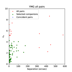
We searched the Gaia archive for binary companions within 10 arcminutes of each of our primaries. We then used the astrometric difference defined in Equation 2 to estimate the significance of the difference in proper motion and parallax and again selected only binaries with $n_{\sigma}<5$. To prevent us being overwhelmed by coincident pairings with unrelated stars with poor astrometric solutions, we excluded any star with a parallax error larger than 0.5 milliarcseconds. We also excluded any pairing where the primary star met this condition. We list only our selected 300–3000 AU pairs in the printed version of Table 7. The online version of this table contains all of our selected YMG binaries.

Figure 8: The pair separation distribution for our three other clusters/populations. Top row: pairs with bona-fide YMG members of Gagné & Faherty (2018) and Gagné et al. (2018) middle row: pairs with Hyades members from Lodieu et al. (2019b) and bottom row: pairs with Pisces-Eridanus members from Meingast et al. (2019), bottom row:. Left: The number of pairs with $n_{\sigma}<5$. Right: All pairs with members from our other clusters/populations plotted alongside an offset pairing populations created using the method of Lépine & Bongiorno (2007). Note the lack of coincident pairs with $n_{\sigma}<5$ below 200 arcseconds for the Young Moving Groups, 120 arcseconds for the Hyades and 400 arcseconds for Pisces-Eridanus and. In all cases we exclude pairs where either component has a parallax error above half a milliarcsecond.

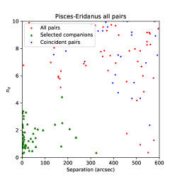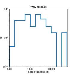
Deacon et al. (2016) suggest that chance alignments between moving group members at similar separations to our search will be relatively rare due to their low density on the sky. To test for chance alignments with field stars we used the offset pairing method of Lépine & Bongiorno (2007). In this we moved the YMG members by two degrees in Right Ascension and re-ran our pairing analysis. This should result in only chance alignments with unrelated stars. As shown in Figure 8 there are no coincident pairs from the Lépine & Bongiorno (2007) offset method with $n_{\sigma}<5$ within 600” and there is no obvious increase in the number of pairs with YMG members with separation below 200”. This suggests our binary sample is free of chance alignments for separations under 200”. We note a number of close pairs with $5<n_{\sigma}<$10. These all appear to have at least one component with an elevated RUWE value and have higher values of $n_{\sigma}$ due to discrepant parallax values. These could well be binaries where one component is itself a close binary leading to an inaccurate astrometric solution. We include these binaries in our list of pairs but flag them as having higher $n_{\sigma}$ values. While these binaries are likely true, bound systems, we exclude them from our binary frequency analysis as to do otherwise would be inconsistent. As a result our Young Moving Group wide binary fractions are likely underestimates.

We estimated our completeness using the method outlined in Section 4.1. We also restricted ourselves to pairs wider than two arcseconds as we are relatively complete at such separations. We divided our binary fraction analysis into three separation bins, 30-300 AU, 300-3000 AU and 3000-10000 AU. Our lower and upper separation limits and the varying distances of our target stars meant that we sometimes did not cover all of each of our three projected separation ranges for all stars. In each projected separation range we then summed the product of the completeness and the log-separation range covered for each star. This was then the denominator for our binary fraction calculations. Our numerator was the number of companions found in each projected separation range. As before we calculated the binary fractions for all stars, FGK stars and M dwarfs. The results are shown in Table 8. We find that in the 300–3000 AU projected separation range, FGK stars in young moving groups have a binary fraction of 14.6$\pm^{4.4}_{3.5}$%, higher than we found in our open clusters. Our M dwarf primary sample is very small so while we find very high wide binary fractions for Young Moving Groups, these binary fractions are highly uncertain.

5.2 Comparison with the Hyades

In our work on open clusters we have selected members of three open clusters and have looked for wide binary companions in all three. One additional check we can make is by comparing with the sample in the Hyades, cluster similar in age to Praesepe (750 Myr; Brandt & Huang 2015a) using members identified by Lodieu et al. (2019b). While this work relies on the same Gaia dataset as our studies of our three open clusters, it uses a different statistical method, the method used in our YMG search above, for identifying companions. The Hyades is also a much closer cluster ($\sim$47 pc) rather than the larger distances ($>$130 pc) for our three other clusters. This means that any bias against close pairs which we have for some reason missed will likely manifest itself in binaries with smaller projected separations than it would in our three clusters.

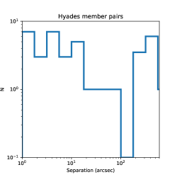
We searched the Gaia archive for co-moving companions within 600 arcseconds of Lodieu et al. (2019b)’s Hyades members, following the authors’ suggestions and restricting ourselves to objects within 30 pc of the cluster centre. As with our YMG companion search, we excluded objects with parallax uncertainties greater than half a milliarcsecond. There will be two possible sources of contamination for Hyades binaries, chance alignments of cluster members and chance alignments with field stars. To estimate the contamination from chance alignments with other Hyades members we paired Hyades members from Lodieu et al. (2019b) together and applied our $n_{\sigma}<5$ cut. A histogram of these pairings is shown in the left-hand panel of Figure 8. Chance alignments with other cluster members should increase with separation, just like in our three open clusters. We do not see any clear ramp-up in numbers below 120 arcseconds. This indicates this region is free of chance alignments of cluster members.

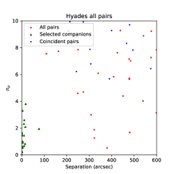
We repeated the chance alignment with field star analysis from the previous section. We found that out to pairing distances of eight arcminutes there were no chance alignments with $n_{\sigma}<5$. Hence we believe a sample of pairs that meet these criteria will be relatively free of contamination. The middle-right-hand panel of Figure 8 shows our selected companions along with the population of chance alignments. There is a clear distinction in this diagram between our pairs and the chance alignments.

We identified 37 wide binary systems in the Hyades that have separations less than 120 arcseconds and $n_{\sigma}<5$. Of those, five have primaries in our FGK mass range and have projected separations in the 300-3000 AU range. We list these pairs in Table 9 with our full list of pairs available in the electronic version of the table.

We estimated our completeness using the method outlined in Section 4.1 using the mass-absolute magnitude relation used by Lodieu et al. (2019b) for Hyades members. We also restricted our analysis to pairs wider than two arcseconds as our census is relatively complete at such separations. However we note that there are 12 binary pairs with separations below our two arcsecond lower limit, the majority of which are M dwarf primaries. We divide our binary fraction analysis into two separation bins, 30-300 AU and 300-3000 AU. We do not detect any binaries with FGK or M primaries in the 3000-10000 AU range (although we have one binary with an A star primary). Hence we measure binary fractions of zero in this range. We have no binaries wider than 3500 AU, suggesting binaries wider than this are rare or lacking in the Hyades. We followed the same process outlined in the previous section and calculated the binary fractions for FGK stars and M dwarfs. The results are shown in Table 8. The binary fractions of both FGK and M stars in the 300-3000 AU range agree well with the number found in our three open clusters.

Table 7: The multiple systems found for Young Moving Group members from Gagné & Faherty (2018) and Gagné et al. (2018). Here we list only the objects with primaries which fell into our FGK mass range, had $n_{\sigma}<5$ and projected separations in the 300-3000 AU range with projected separations greater than two arcseconds.

Gaia ID	Position	$\mu_{\alpha}\cos{\delta}$	$\mu_{\delta}$	$\pi$	$G$	Projected		Other name
						Separation
	(Eq.=J2000 Ep.=2015.5)	(mas/yr)	(mas/yr)	(mas)	(mag)	(”)	(AU)
AB Dor
374400957846408192	01:03:40.30 +40:51:26.7	126.9$\pm$0.1	-161.3$\pm$0.1	32.2$\pm$0.1	10.1	27.9	864.9	G 132-50
374400893423204992	01:03:42.23 +40:51:13.5	132.9$\pm 0.1$	$-$155.9$\pm$0.01	32.5$\pm$0.1	12.3			G 132-51 B
374400893422315648	01:03:42.45 +40:51:13.2	130.4$\pm$0.2	-162.5$\pm$0.2	32.7$\pm$0.1	13.2			G 132-51 A
248004472671281664	03:33:13.59 +46:15:23.8	68.6$\pm$0.1	-175.3$\pm$0.1	27.5$\pm$0.1	8.0	9.5	346.1	HD 21845
248004472671505152	03:33:14.15 +46:15:16.3	69.0$\pm$0.1	-172.6$\pm$0.1	27.5$\pm$0.1	10.5			HD 21845 B
4795598309045006208	05:36:56.89 -47:57:52.9	23.3$\pm$0.1	-1.1$\pm$0.1	40.6$\pm$0.1	7.5	18.3	449.6	UY Pic
4795596831576255488	05:36:55.14 -47:57:47.9	28.7$\pm$0.1	3.4$\pm$0.1	40.6$\pm$0.1	9.3			HIP 26369
4802947444765743104	05:37:12.93 -42:42:55.8	8.4$\pm$0.1	-10.3$\pm$0.1	12.5$\pm$0.1	9.5	4.0	320.8	HD 37551A
4802947444765742848	05:37:13.26 -42:42:57.5	11.9$\pm$0.1	-8.6$\pm$0.1	12.4$\pm$0.1	10.3			HD 37551B
beta Pic
107774202769886848	02:17:25.39 +28:44:41.0	87.1$\pm$0.1	-74.1$\pm$0.1	25.1$\pm$0.1	6.9	13.8	547.2	HD 14082
107774198474602368	02:17:24.84 +28:44:29.3	86.0$\pm$0.1	-71.1$\pm$0.1	25.2$\pm$0.1	7.6			HD 14082B
132362959259196032	02:27:29.35 +30:58:23.5	79.5$\pm$0.1	-72.0$\pm$0.1	24.4$\pm$0.1	9.7	22.0	903.2	BD+30 397
132363027978672000	02:27:28.15 +30:58:39.2	82.7$\pm$0.1	-73.5$\pm$0.1	24.4$\pm$0.1	11.4			BD+30 397
5935776714456619008	16:57:20.24 -53:43:32.9	-21.0$\pm$0.2	-84.1$\pm$0.1	19.8$\pm$0.1	11.3	11.0	555.4	TYC 8726-1327-1
5935776710115544832	16:57:21.41 -53:43:29.2	-16.2$\pm$0.2	-85.7$\pm$0.1	19.8$\pm$0.1	15.9			2MASS J16572144-5343277
5811866422581688320	17:17:25.45 -66:57:05.9	-21.5$\pm$0.1	-137.1$\pm$0.1	32.8$\pm$0.1	6.4	34.1	1040.7	HD 155555 A
5811866358170877184	17:17:31.25 -66:57:07.7	-14.8$\pm$0.1	-145.1$\pm$0.1	33.0$\pm$0.1	11.4			HD 155555 C
6702775135228913280	18:03:03.41 -51:38:57.8	2.3$\pm$0.1	-86.1$\pm$0.1	20.2$\pm$0.1	6.9	6.5	322.1	HD 164249 A
6702775508886369408	18:03:04.11 -51:38:57.7	5.8$\pm$0.1	-95.0$\pm$0.1	20.2$\pm$0.1	12.3			HD 164249 B
6400161703868444800	21:21:24.75 -66:54:58.9	95.7$\pm$0.1	-100.3$\pm$0.1	31.3$\pm$0.1	8.7	26.5	836.1	V390 Pav
6400160947954197888	21:21:28.99 -66:55:07.8	116.0$\pm$0.7	-85.3$\pm$0.8	31.7$\pm$0.4	10.0			TYC 9114-1267-1
Carina Near
3466924200065405184	11:56:42.10 -32:16:05.5	-172.0$\pm$0.1	-8.2$\pm$0.1	28.2$\pm$0.1	7.5	18.7	664.2	HD 103743
3466924200065405824	11:56:43.56 -32:16:02.8	-178.9$\pm$0.1	-6.7$\pm$0.1	28.1$\pm$0.1	7.6			HD 103742
1541667932396172800	12:28:04.18 +44:47:39.4	-181.8$\pm$0.1	-4.7$\pm$0.1	22.0$\pm$0.1	7.3	9.7	442.3	HD 108574
1541667932396172416	12:28:04.54 +44:47:30.5	-180.4$\pm$0.1	0.4$\pm$0.1	21.9$\pm$0.1	7.9			HD 108575
Tuc Hor
4714764481913306496	02:07:26.31 $-$59:40:46.2	92.7$\pm$0.1	$-$18.3$\pm$0.01	21.9$\pm$0.1	7.4	52.3	2387	HD 13246
4714764447553568640	02:07:32.40 $-$59:40:21.4	93.6$\pm$0.1	$-$21.7$\pm$0.1	22.0$\pm$0.1	9.9			CD-60 416
4742040410461492096	02:41:47.00 $-$52:59:52.6	97.8$\pm$0.1	$-$14.2$\pm$0.1	22.8$\pm$0.1	9.7	22.2	972	CD-53 544
4742040513540707072	02:41:47.47 $-$52:59:30.8	93.5$\pm$0.1	$-$11.6$\pm$0.2	23.0$\pm$0.1	11.1			AF Hor
4842275841819363200	04:00:32.08 $-$41:44:54.4	68.2$\pm$0.1	$-$7.0$\pm$0.1	19.2$\pm$0.1	8.2	8.8	456	HD 25402 A
4842275837523665664	04:00:32.35 $-$41:45:02.6	71.7$\pm$0.1	$-$0.4$\pm$0.1	19.19$\pm$0.1	12.3			HD 25402 B
4891725758804030208	04:38:44.01 $-$27:02:02.0	56.3$\pm$0.1	$-$10.9$\pm$0.1	18.3$\pm$0.1	8.3	23.0	1255	HD 29615 A
4891725758804028672	04:38:45.73 $-$27:02:02.2	56.8$\pm$0.1	$-11.7\pm$0.1	18.4$\pm$0.1	14.4			HD 29615 B
TWA
5399220743767211776	11:21:17.13 -34:46:45.8	-66.0$\pm$0.1	-18.1$\pm$0.1	16.7$\pm$0.1	10.9	5.1	303.5	CD-34 7390 A
5399220743767211264	11:21:17.36 -34:46:50.0	-69.0$\pm$0.1	-16.9$\pm$0.1	16.7$\pm$0.1	10.9			CD-34 7390 B

Table 8: The binary fractions for different types of stars in our six young moving groups, the Hyades and the Pisces-Eridanus stream. We use uncertainty estimates calculated with the relations of Gehrels (1986) as these are more appropriate for small number statistics. In each case we estimate the binary fraction divided by the log separation range covered $\frac{df_{bin}}{d\log_{10}x}$. Our two subranges cover approximately FGK dwarfs ($0.5<M/M_{\odot}<1.5$) and M dwarfs ($M<0.5M_{\odot}$). For Pisces Eridanus we only cover binaries with primaries that are approximately FGK dwarfs ($0.5<M/M_{\odot}<1.5$) as there are no lower-mass objects in the membership list of Meingast et al. (2019). The x-axis error bars represent the projected separation range covered.

	$N_{companions}$	$N_{stars}$	$\sum Completeness\times d\log r$	$\frac{df_{bin}}{d\log_{10}x}$
Young Moving Groups
FGK stars
30-300 AU	6	130	54.6	11.0$\pm^{6.7}_{4.8}$%
300-3000 AU	17	130	116.5	14.6$\pm^{4.4}_{3.5}$%
3000-10000 AU	1	130	49.5	2.0$\pm^{4.9}_{1.7}$%
M stars
30-300 AU	4	19	10.1	39.6$\pm^{32.0}_{19.2}$%
300-3000 AU	3	19	12.4	24.2$\pm^{23.7}_{13.4}$%
3000-10000 AU	1	19	2.9	34.5$\pm^{65.5}_{30.0}$%
Hyades
FGK stars
30-300 AU	7	196	66.6	10.5$\pm^{5.7}_{3.9}$%
300-3000 AU	5	196	176.6	2.5$\pm^{2.0}_{1.2}$%
3000-20000 AU	0	196	98.4	0.0$\pm^{2.0}_{0.0}$%
M stars
30-300 AU	8	390	94.0	8.5$\pm^{4.2}_{3.0}$%
300-3000 AU	3	390	232.4	1.3$\pm^{1.3}_{0.7}$%
3000-20000 AU	0	390	134.2	0.0$\pm^{1.5}_{0.0}$%
Pisces-Eridanus
FGK stars
300-3000 AU	22	249	204.9	10.7$\pm^{2.8}_{2.3}$%
3000-20000 AU	11	249	183.6	6.0$\pm^{2.4}_{1.8}$%

Table 9: Wide companions to Hyades members listed in Lodieu et al. (2019b). Here we list only the companions where the primaries have mass estimates in the $0.5<M/M_{\odot}<1.5$ range and with projected separations in the 300-3000 AU range with projected separations greater than two arcseconds. A full version of this table with all pairs will be available electronically.

Gaia ID	Position	$\mu_{\alpha}\cos{\delta}$	$\mu_{\delta}$	$\pi$	$G$	Projected
						Separation
	(Eq.=J2000 Ep.=2015.5)	(mas/yr)	(mas/yr)	(mas)	(mag)	(”)	(AU)
108421608959951488	02:58:05.48 +20:40:07.0	234.0$\pm$0.1	$-$31.3$\pm$0.1	30.6$\pm$0.1	5.7	14.7	479.0
108421402801188864	02:58:06.45 +20:40:01.3	238.1$\pm$0.2	$-$24.5$\pm$0.2	30.6$\pm$0.1	13.5
125343573948444800	03:13:03.02 +32:53:46.3	184.5$\pm$0.1	$-$61.9$\pm$0.1	25.3$\pm$0.1	8.0	10.6	419.2
125343608307015296	03:13:03.83 +32:53:49.3	186.2$\pm$0.1	$-$65.6$\pm$0.1	25.4$\pm$0.1	12.9
56447041481918720	03:37:33.53 +17:51:14.1	170.6$\pm$0.1	$-$30.2$\pm$0.1	25.8$\pm$0.1	11.7	16.2	626.3
56447037184877824	03:37:34.09 +17:51:00.0	170.5$\pm$0.1	$-$27.9$\pm$0.1	25.6$\pm$0.1	12.1
50756411675761920	03:49:06.16 +18:50:11.6	104.5$\pm$0.1	$-$20.9$\pm$0.1	16.4$\pm$0.1	12.2	9.7	595.4
50756415973201152	03:49:05.54 +18:50:15.8	106.2$\pm$0.1	$-$23.1$\pm$0.1	16.6$\pm$0.1	14.3
145293181643038336	04:26:18.61 +21:28:13.0	103.2$\pm$0.1	$-$38.4$\pm$0.1	20.7$\pm$0.1	7.2	11.1	536.9
145293181643038208	04:26:19.31 +21:28:07.5	105.8$\pm$0.2	$-$40.3$\pm$0.1	20.9$\pm$0.1	15.1

Table 10: Wide companions to Pisces-Eridanus stream members listed in Meingast et al. (2019). Here we only list objects in the 300-3000 AU projected separation range with projected separations greater than two arcseconds. A full version of this table with all pairs will be available electronically.

Gaia ID	Position	$\mu_{\alpha}\cos{\delta}$	$\mu_{\delta}$	$\pi$	$G$	Projected
						Separation
	(Eq.=J2000 Ep.=2015.5)	(mas/yr)	(mas/yr)	(mas)	(mag)	(”)	(AU)
2741273390752119680	00 18 42.99 +05 06 35.6	20.0$\pm$0.1	$-$15.8$\pm$0.0	8.3$\pm$0.0	13.3	2.5	301
2741273395049220992	00 18 43.13 +05 06 34.3	19.5$\pm$0.1	$-$16.1$\pm$0.1	8.4$\pm$0.0	14.2
2799470060173799680	00 23 04.65 +21 27 50.9	13.1$\pm$0.1	$-$18.1$\pm$0.1	5.9$\pm$0.1	12.4	3.6	615
2799470060175375872	00 23 04.44 +21 27 52.9	13.3$\pm$0.2	$-$18.0$\pm$0.2	6.0$\pm$0.1	16.7
2528797033588184960	00 44 19.62 $-$04 23 56.9	20.2$\pm$0.1	$-$11.1$\pm$0.1	10.1$\pm$0.1	8.7	8.3	820
2528796277673941376	00 44 20.05 $-$04 24 02.1	20.9$\pm$0.2	$-$10.8$\pm$0.1	10.1$\pm$0.1	15.1
4975223840046231424	00 47 38.48 $-$47 41 45.8	24.6$\pm$0.0	22.4$\pm$0.0	12.4$\pm$0.0	11.5	9.3	746
4975223840048745472	00 47 39.36 $-$47 41 48.6	24.0$\pm$0.1	22.4$\pm$0.1	12.3$\pm$0.1	15.2
2577307864562003456	01 02 29.70 +06 59 54.5	14.1$\pm$0.1	$-$17.3$\pm$0.1	9.8$\pm$0.1	9.8	12.6	1280
2577307860266860800	01 02 30.41 +07 00 01.3	15.0$\pm$0.5	$-$16.4$\pm$0.2	10.0$\pm$0.2	17.9
2590688680553786368	01 24 29.20 +15 30 36.2	13.3$\pm$0.1	$-$27.1$\pm$0.1	9.8$\pm$0.0	10.2	3.6	366
2590688680553786240	01 24 29.27 +15 30 39.7	19.4$\pm$0.4	$-$25.6$\pm$0.1	9.8$\pm$0.1	15.1
2508964107269556864	01 42 37.20 $-$00 47 50.9	11.0$\pm$0.1	$-$12.2$\pm$0.1	8.9$\pm$0.1	12.2	4.7	522
2508964111565146752	01 42 37.02 $-$00 47 54.7	11.8$\pm$0.5	$-$15.0$\pm$0.3	9.1$\pm$0.3	17.1
5141461678818746880	01 59 17.21 $-$17 46 38.0	10.0$\pm$0.1	$-$0.4$\pm$0.1	11.5$\pm$0.0	12.8	7.7	667
5141461683110761728	01 59 17.45 $-$17 46 44.8	9.7$\pm$0.0	$-$0.6$\pm$0.0	11.4$\pm$0.0	13.4
2462582789799726336	01 59 54.07 $-$09 30 16.6	7.9$\pm$0.1	$-$5.7$\pm$0.1	8.0$\pm$0.1	10.8	6.0	748
2462582794095085056	01 59 53.73 $-$09 30 19.6	1.4$\pm$3.3	$-$5.3$\pm$2.7	1.9$\pm$1.8	20.4
24667616384335872	02 27 47.44 +11 14 27.3	3.6$\pm$0.1	$-$19.5$\pm$0.1	7.6$\pm$0.0	10.7	15.4	2036
24667616384335744	02 27 48.49 +11 14 26.5	4.1$\pm$0.1	$-$20.0$\pm$0.1	7.6$\pm$0.1	15.1
5155187986271622912	03 20 33.29 $-$14 16 58.4	$-$0.7$\pm$0.1	$-$3.0$\pm$0.1	7.5$\pm$0.1	12.3	2.4	323
5155187986271622784	03 20 33.17 $-$14 16 56.7	$-$1.7$\pm$0.1	$-$2.1$\pm$0.1	7.3$\pm$0.1	13.4
5085954625291316224	03 30 22.88 $-$24 22 26.1	$-$0.0$\pm$0.0	2.6$\pm$0.0	8.5$\pm$0.0	12.1	3.7	441
5085954625291316096	03 30 22.74 $-$24 22 22.8	$-$1.0$\pm$0.1	2.4$\pm$0.1	8.5$\pm$0.1	15.1
3193559873957065472	03 55 08.93 $-$10 10 11.8	$-$3.5$\pm$0.1	$-$1.3$\pm$0.1	5.6$\pm$0.0	9.4	12.8	2300
3193559839597327360	03 55 08.08 $-$10 10 14.7	$-$3.5$\pm$0.1	$-$1.4$\pm$0.1	5.7$\pm$0.1	16.6
5092558979319804672	04 13 00.24 $-$19 51 17.2	$-$6.1$\pm$0.1	2.5$\pm$0.1	5.9$\pm$0.0	9.1	17.1	2874
5092558979319804928	04 12 59.03 $-$19 51 18.6	$-$6.2$\pm$0.2	3.0$\pm$0.2	6.5$\pm$0.2	17.0
3205573756476323328	04 23 54.59 $-$02 33 43.4	$-$7.1$\pm$0.1	$-$5.9$\pm$0.0	6.4$\pm$0.0	11.6	16.7	2604
3205573756476257792	04 23 54.71 $-$02 33 59.9	$-$6.7$\pm$0.2	$-$5.6$\pm$0.1	6.5$\pm$0.1	17.1
3198734278756825856	04 26 27.10 $-$07 39 39.7	$-$9.6$\pm$0.0	$-$4.9$\pm$0.0	6.2$\pm$0.0	11.5	3.3	535
3198734278756825984	04 26 26.91 $-$07 39 41.6	$-$8.2$\pm$0.1	$-$4.8$\pm$0.0	6.2$\pm$0.0	14.5
3185678437170300800	04 34 42.76 $-$08 57 18.5	$-$9.2$\pm$0.0	$-$4.8$\pm$0.0	6.0$\pm$0.0	11.9	6.9	1143
3185678437170301056	04 34 42.38 $-$08 57 22.4	$-$8.8$\pm$0.0	$-$5.8$\pm$0.0	6.1$\pm$0.0	13.7
2709158614610269312	22 30 54.93 +06 09 13.8	18.3$\pm$0.1	$-$12.1$\pm$0.1	6.0$\pm$0.0	11.7	11.7	1941
2709158687624627584	22 30 54.15 +06 09 15.1	18.0$\pm$0.2	$-$11.2$\pm$0.2	6.2$\pm$0.1	15.8
2623655475128272384	22 38 32.87 $-$06 12 49.4	24.8$\pm$0.1	$-$9.8$\pm$0.1	7.4$\pm$0.1	10.3	6.7	904
2623655470833544704	22 38 32.95 $-$06 12 42.7	29.3$\pm$0.1	$-$9.2$\pm$0.1	7.6$\pm$0.1	12.9
2596395760081700608	22 39 53.53 $-$16 36 23.3	24.5$\pm$0.1	$-$4.4$\pm$0.1	7.9$\pm$0.0	11.5	3.2	408
2596395764377286272	22 39 53.74 $-$16 36 24.2	24.0$\pm$0.2	$-$1.8$\pm$0.3	7.7$\pm$0.1	15.6
2625503165763607808	22 43 16.91 $-$03 03 06.6	25.9$\pm$0.1	$-$12.2$\pm$0.1	6.9$\pm$0.1	10.8	5.1	746
2625503165766158848	22 43 17.18 $-$03 03 09.8	25.4$\pm$0.4	$-$11.4$\pm$0.4	5.5$\pm$0.4	18.2
2612073116562162304	22 52 26.88 $-$05 05 12.5	25.8$\pm$0.1	$-$10.3$\pm$0.1	7.8$\pm$0.0	12.1	2.7	344
2612073082202424320	22 52 26.71 $-$05 05 13.4	22.5$\pm$0.1	$-$11.0$\pm$0.1	7.7$\pm$0.0	14.3
2659702787750762624	23 25 32.83 +03 32 42.4	18.1$\pm$0.1	$-$12.6$\pm$0.1	7.0$\pm$0.1	12.8	13.8	1966
2659702787750762752	23 25 32.06 +03 32 34.7	18.1$\pm$0.1	$-$12.1$\pm$0.1	7.0$\pm$0.0	12.9

5.3 Comparison with the Pisces-Eridanus stream

The Pisces-Eridanus stream is a kinematic structure identified by Meingast et al. (2019) in Gaia data. They estimated that this stream is a $\sim$1 Gyr-old dispersed remnant of a single star formation event that extends to 400 pc in length. More recently Curtis et al. (2019) have used gyrochronology to estimate an age of $\sim$125 Myr. Moreover Curtis et al. (2019) suggest that the Pisces-Eridanus stream formed in a dispersed manner with multiple cores, similar to nearby young associations. Hence this stream could represent a more dispersed star formation event which lies at a similar distance to the Pleiades and has a similar age. We set out to measure the wide binary fraction in this stream as any deviation from the Pleiades wide binary fraction would hint at an environmental dependence in the formation and/or survival of wide binaries.

We repeated the analysis we did for the Hyades and the Young Moving Groups using the membership list from Meingast et al. (2019). Again we examined coincident pairs between members of the stream and also searched for coincident pairs using the offset pairing method of Lépine & Bongiorno (2007). Figure 8 shows both of these analyses. It is clear that there is no significant population of chance alignments out to separations of 400”. We list our 300-3000 AU pairs in the printed version of Table 10 with the full list in the electronic version of this table. We estimated the masses of both components of each pair using the same PARSEC models we used for the Pleiades (as the Curtis et al. 2019 age suggest this cluster is the same age as Pisces-Eridanus). The members listed in Meingast et al. (2019) almost all fall into the $0.5<M/M_{\odot}<1.5$ range. Hence we are only able to calculate the binary fraction for FGK stars. We do this using the same incompleteness analysis as was used for the Hyades and the Young Moving Groups. Our binary frequency calculations are shown in Table 8. As with the Young Moving Groups we find that the there is an excess of binaries in the 300-3000 AU range with 10.7$\pm^{2.8}_{2.3}$% of FGK stars having companions in the 300-3000 AU projected separation range compared to our value of 3.6$\pm^{0.8}_{0.7}$% in our three open clusters.

6 Discussion

6.1 The environmental dependence of the wide binary fraction

Our results are plotted, along with the literature values and our Young Moving Group FGK binary fractions in Figure 9. As discussed in the introduction, studies of close unresolved binarity in our three clusters indicate that the binary fraction matches the field distribution. As these studies mostly concentrate on FGK stars we restrict ourselves to pairs where the our primaries have a mass range between 0.5 and 1.5 solar masses. Hillenbrand et al. (2018) refer to their primaries as KM stars but the vast majority have mass estimates in the 0.5–0.9 $M_{\odot}$ range. We recalculate the uncertainties in the literature results using Gehrels (1986) so that they are comparable with our uncertainty estimates. We also calculated the combined cluster binary fraction from Patience et al. (2002) using the figures in their Table A1 and multiplying by a factor of $\frac{4}{3}$. This latter factor takes into account possible incompleteness as Patience et al. (2002) state they are likely complete for $q>0.25$ so assuming a flat mass ratio distribution they should have detected 75% of binaries. We divide by the log separation range each study covers so that we have comparable values of $\frac{df_{bin}}{d\log_{10}x}$ (where $x$ is the angular separation).

It is clear that for the Pleiades, Praesepe and the combined result for all three clusters, the wide binary fraction for FGK dwarfs falls below that expected in the field. The field binary fraction falls away at higher separations and our open cluster 300–3000 AU wide binary fraction is more comparable with the field value found at separations wider than 2000 AU by Tokovinin & Lépine (2012). Alpha Per has a higher, but more uncertain binary fraction indicating that this higher value could be due to noise. The deficit in wide companions in two of our three clusters and in the combined cluster result appear to be significant at the $\sim 3\sigma$ level. By contrast the Pisces-Eridanus and YMG binary fractions seems to lie slightly above or on the field distribution. It is possible that we have somehow biased ourselves against close pairs. However we have shown in Section 4.1 that cluster members can be reliably detected at separations wider than two arcseconds. Hence we suggest that this deficit in the number of wide binaries in our cluster could be due to some level of dynamical processing of wide binaries in open clusters. If this is correct then we would expect that the field population of wide binaries would have formed (and survived) preferentially in lower-density formation environments, albeit with some contribution from denser clusters as well.

Figure 9: The binary fractions from this work, Raghavan et al. (2010), Patience et al. (2002) (incorporating the results of Bouvier et al. 1997), Hillenbrand et al. (2018) and Tokovinin & Lépine (2012). Left: It appears that while closer binaries in Alpha Per, the Pleiades, Praesepe and the Hyades are in agreement with the field population, there is a deficit of wider binaries. Right: Conversely the less dense Young Moving Groups and Pisces-Eridanus stream show wide binary fractions at or above the field values.

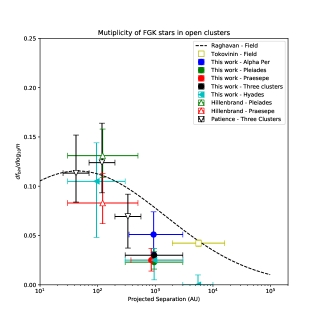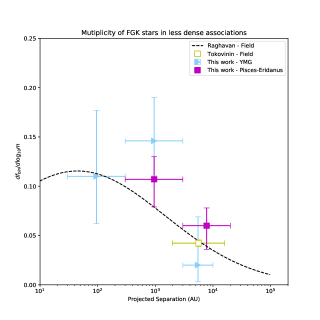We can use the approach taken by Brandner & Köhler (1998) and Patience et al. (2002) to estimate the origins of field wide binaries and of stars in general. These works proposed a model where there were two possible origins for wide binaries, Pleiades-like clusters and lower density star forming regions similar to Pisces-Eridanus. This is an extreme model as there is actually a continuum of stellar formation environments with only 7% of embedded clusters resulting in Pleiades-like open clusters (Lada & Lada, 2003). There are also more extreme dense, high-mass star forming regions than the progenitor of the Pleiades with multiple clusters in the Milky Way having masses over 10⁴ M_⊙ (Portegies Zwart et al., 2010) which will be so dense that the average separation between members in the centre will be of the order of a few thousand AU. Nonetheless, if we assume that the binary fraction of field stars follows the distribution of Raghavan et al. (2010) this would mean that in our 300-3000 AU separation range we would expect an occurrence rate of $\frac{df_{bin}}{d\log_{10}x}=7.8\%$. In the Pleiades we find $\frac{df_{bin}}{d\log_{10}x}=$2.3$\pm^{1.1}_{0.7}$% in the same separation while in Pisces-Eridanus we have $\frac{df_{bin}}{d\log_{10}x}=$10.7$\pm^{2.8}_{2.3}$%. We then assume the aforementioned toy model of star formation with only two environments, the progenitor environment of the Pleiades and the progenitor environment of Pisces-Eridanus. In this model $X\%$ of stars would form in the former environment and $100-X\%$ would form in the latter. We used a numerical simulation where we drew a hundred thousand random binomial distributions with our calculated 300-3000 AU binary fractions for both the Pleiades and Pisces-Eridanus and with the correct number of stars in each around which we could detect binaries. For each of these hundred thousand simulated populations we calculated $X$ and from the distribution of $X$ calculated the median and standard deviation around that median. These simulations imply that $X=38\pm^{13}_{16}$% of stars form in Pleiades-progenitor-like environments and the remainder in less dense, more distributed environments. This is below the 70$\pm^{10}_{15}\%$ or 80% figure calculated by Patience et al. (2002) who assumed that the binary separation distributions in star forming regions would equate to the final binary separation distributions that would make their way from those star forming regions into the field. We again note that this method for estimating the origin of wide binaries forces star formation environments into two distinct types when there is a spectrum of star formation environments.

Our work suggests that the products of low density star formation regions have higher wide binary fractions than the products of higher-mass star-forming clusters. In the lower-density Taurus-Auriga (Kraus et al., 2011) and Ophiuchus (Cheetham et al., 2015) regions the wide binary fraction appears to be at or above the field level. The best nearby comparator we have for more massive star forming regions is the Trapezium Cluster within the Orion Nebula Cluster (ONC). Lada & Lada (2003) used the low number of wide binaries found by Scally et al. (1999) as evidence for the rapid destruction of wide binaries in the progenitors of open clusters. However recently Jerabkova et al. (2019) found a wide (1000–3000 AU) binary fraction of 5% with primaries that are mostly M dwarfs. This work, like that of Scally et al. (1999) covered a much larger area than just the central Trapezium Cluster itself. In a survey of the central 20 arcmins of the ONC Reipurth et al. (2007) found a binary fraction of 8.8$\pm$1.1% between 67.5 and 675 AU, again with a sample dominated by M dwarfs (83%). Even accounting for the ONC’s younger age (1–3 Myr; Beccari et al. 2017) the vast majority of these objects would have comparable masses to our M dwarf sample in our clusters. We find that across our three clusters that 1.4$\pm^{0.4}_{0.3}$% of M dwarfs are the primary stars in binary systems with separations in the 300–3000 AU range. We recalculate the Reipurth et al. (2007) binary fraction in their two widest bins 250–675 AU and find a binary fraction of $\frac{df_{bin}}{d\log_{10}x}=5.4\pm^{1.6}_{1.3}$%. Reipurth et al. (2007) found the ratio of binaries with projected separations wider than $\sim$250 AU to those wider than this limit varied with the distance from the centre of the Trapezium Cluster with relatively few wide binaries in the inner 400 arcseconds of the cluster. Reipurth et al. (2007) also note that their survey of the central region of the ONC has roughly 2.2 times fewer wide binaries than studies of looser T-Tauri associations.

We note that using a total mass of 735 M_⊙ and a half-mass radius of 3.66 pc (Pinfield et al., 1998) the hard-soft boundary in the Pleiades today would be roughly 1500 AU. However much of the dynamical processing of a cluster like the Pleiades would likely have been done when it was younger and possibly more compact. See Parker et al. (2009)’s work on an ONC-like cluster.

6.2 Other possible explanations

We have found that open clusters such as the Alpha Per, the Hyades, the Pleiades and Praesepe host fewer wide binaries than associations which likely formed in less dense star forming regions such as Young Moving Groups and the Pisces-Eridanus stream. There are a number of arguments against the results of our survey being evidence for an environmental dependence in the wide binary frequency. It could be that we are missing a large number of binaries in the open clusters due to small-scale incompleteness in the Gaia data. However we have shown that the quality of Gaia data are not affected by a close companion wider than three arcseconds and only minimally affected in the 2”–3” range. Furthermore if small-scale incompleteness were to affect the Pleiades and suppress its binary fraction, one would also expect it to affect the Pisces-Eridanus stream (which lies at a similar distance) in a similar way. Finally, we have shown that the Hyades also has a suppressed wide binary fraction at $>$300 AU. For this to be caused by small-scale incompleteness the Gaia data would need to be incomplete at separations of 6 arcseconds. We have found no evidence to support such incompleteness.

It could be argued that the deficit in wide binaries in open clusters would be replenished by the cluster members capturing other cluster members as the cluster dissolves. Indeed it has been suggested by (Kouwenhoven et al., 2010) this could be origin of 1–30% of $>$1000 AU wide binaries. However we note that the Hyades, a cluster which has dissolved to the point where capture between members seems incredibly unlikely, also has a deficit of wide binaries similar to the other open clusters.

It could be possible that systems which currently have separations below our 300 AU lower bound will evolve into wider binaries by the time they reach field age. Elliott & Bayo (2016) suggest a model based on work by Reipurth & Mikkola (2012) where wide binaries are hidden higher-order multiples and slowly increase their separation over time, albeit at younger ages than our open clusters. We think this process will be unlikely to have affected our results as the deficit in wide binaries appears similar between the Pleiades (125 Myr) and the Hyades & Praesepe ($\sim$750 Myr). Further we also note that the Pleiades and the Pisces-Eridanus stream are approximately the same age and show significantly different wide binary fractions, suggesting an environment-dependent rather than age-dependent effect. It is however true that further evolution of wide binary systems before they reach field age would alter the fraction of wide binaries each star formation environment would donate to the field.

7 Conclusions

We have shown that there appears to be a deficit of wide (300–3000 AU) binaries in open clusters. This deficit persists over a range of cluster distances, suggesting it is not the product of small-scale incompleteness in the Gaia data release. We also compared to young moving groups and the Pisces-Eridanus stream (both likely products of lower-density, less-clustered star formation events) and found these had wide binary fractions at or above the field level. These results suggest that wide binaries are more likely form and/or survive in low density formation environments than more dense star clusters.

Appendix A Deriving the cluster membership likelihood

We used a similar likelihood method to Deacon & Hambly (2004) (based on previous work such as Sanders 1971 and Hambly et al. (1995)) which fitted likelihood distributions in proper motion space for the cluster and field populations. We used an altered version of this method in proper motion space. First we calculate the expected proper motion of a cluster member at the space position of each star using the $UVW$ velocities quoted in Lodieu et al. (2019a) and coordinate system transformations from the astropy coordinates package (Robitaille et al., 2013). We then project the proper motion of each object to a basis where one direction is parallel to the expected cluster proper motion at the space position of each object and one direction perpendicular ($\mu_{\parallel obs}$ and $\mu_{\perp obs}$). In this basis a cluster member will be expected to have its proper motion entirely in the direction of cluster motion. Thus the total expected proper motion for each cluster member is $\mu_{\parallel exp}$ while $\mu_{\perp exp}=0$. We then subtract the expected proper motion in the direction of cluster motion such that $\Delta\mu_{\parallel}=\mu_{\parallel obs}-\mu_{\parallel exp}$. We then use $\Delta\mu_{\parallel}$ and $\mu_{\perp obs}$ as the basis for our proper motion analysis. The cluster forms a Gaussian distribution around roughly (0,0) while we found that the field population was also a Gaussian centred away from the origin. The width of the cluster distribution will be a combination of the true $UVW$ distribution of the cluster, the range of distances along the line of sight, uncertainties in the expected proper motions and the measurement uncertainties of the proper motions. We also diverge from the method of Deacon & Hambly (2004) by adding a parallax terms to our likelihoods. Here the width of the parallax distribution will be a combination of parallax uncertainty and the line of sight depth of the cluster. As the typical parallax and proper motion uncertainties increase with magnitude we split our analysis into magnitude bins. This allows fainter stars to have higher parallax and proper motion dispersions than brighter stars. We neglect the covariances between proper motion and parallax and assume that the intrinsic proper motion dispersion does not change significantly across the cluster. Assuming the Pleiades is about 10 pc deep we would expect the proper motion dispersion to vary by around 7% with smaller dispersions for other clusters. Our selection only uses proper motions and parallaxes to determine membership probabilities while other methods use the spatial distribution of the stars to calculate membership probabilities. We choose not to do this as we do not want to assume a possibly incorrect functional form for the spatial distribution that could bias our selection.We start by defining a likelihood $\phi$ that is a sum of field and cluster components.

$$\phi=f\phi_{f}+(1-f)\phi_{c}$$ (7)

Where the field component is defined as,

$$\phi_{f}=\frac{c_{\varpi}}{2\pi\Sigma_{\parallel}\Sigma_{\perp}}e^{\big{(}-\frac{(\mu_{\perp}-\mu_{\perp,f})^{2}}{2\Sigma_{\perp}^{2}}-\frac{(\Delta\mu_{\parallel}-\Delta\mu_{\parallel,f})^{2}}{2\Sigma_{\parallel}^{2}}-\frac{\varpi}{\tau_{\varpi}}\big{)}}$$ (8)

Where the proper motion terms parallel and perpendicular to the direction of cluster motion ($\Delta\mu_{\parallel}$ and $\mu_{\perp}$) are Gaussian and the parallax terms ($\varpi$) is a declining exponential. Deacon & Hambly (2004) used a declining exponential for the $\mu_{y}$ term. We chose to use a declining exponential in $\varpi$ after examining a historgram of the parallax values for each the area around each cluster. As we use a declining exponential, we require a normalisation term for $\varpi$

$$c_{\varpi}=\frac{1}{\int_{\varpi_{min}}^{\varpi{max}}e^{-\frac{\varpi}{\tau_{\varpi}}}d\varpi}=\frac{1}{\tau_{\varpi}(e^{-\frac{\varpi_{min}}{\tau_{\varpi}}}-e^{-\frac{\varpi_{max}}{\tau_{\varpi}}})}$$ (9)

For all our clusters we choose limits of $\varpi_{min}=3$ mas and $\varpi_{max}=15$ mas.

We define the cluster component of our likelihood as,

$$\phi_{c}=\frac{1}{(2\pi)^{3/2}\sigma_{\varpi}\sigma_{\perp}\sigma_{\parallel}}e^{\big{(}-\frac{(\mu_{\perp}-\mu_{\perp c})^{2}}{2\sigma_{\perp}^{2}}-\frac{(\Delta\mu_{\parallel}-\Delta\mu_{\parallel c})^{2}}{2\sigma_{\parallel}^{2}}-\frac{(\varpi-\varpi_{c})^{2}}{2\sigma_{\varpi}^{2}}\big{)}}$$ (10)

Where we use Gaussians for both the parallax and both components of the proper motion. Unlike in Deacon & Hambly (2004) we use separate standard deviations for the proper motion components of the Gausssian.

We then find the best fitting parameters by maximising the derivative of the logarithm of the likelihood with respect to each of our likelihood parameters $\Theta$ such that,

$$\sum_{i}\frac{\partial\ln\phi_{i}}{\partial\Theta}=0$$ (11)

This then leads to individual equations

$$f:\sum_{i}\frac{\phi_{f,i}-\phi_{c,i}}{\phi_{i}}=0$$ (12)

$$\sigma_{\perp}:\sum_{i}\frac{\phi_{c,i}}{\phi_{i}}\left(\frac{(\mu_{\perp,i}-\mu_{\perp c})^{2}}{\sigma_{\perp}^{2}}-1\right)$$ (13)

$$\sigma_{\parallel}:\sum_{i}\frac{\phi_{c,i}}{\phi_{i}}\left(\frac{(\Delta\mu_{\parallel,i}-\Delta\mu_{\parallel c})^{2}}{\sigma_{\parallel}^{2}}-1\right)$$ (14)

$$\sigma_{\varpi}:\sum_{i}\frac{\phi_{c,i}}{\phi_{i}}\left(\frac{(\varpi_{i}-\varpi_{c})^{2}}{\sigma_{\varpi}^{2}}-1\right)$$ (15)

$$\mu_{\perp c}:\sum_{i}\frac{\phi_{c,i}}{\phi_{i}}\left(\mu_{\perp,i}-\mu_{\perp c}\right)$$ (16)

$$\Delta\mu_{\parallel c}:\sum_{i}\frac{\phi_{c,i}}{\phi_{i}}\left(\Delta\mu_{\parallel,i}-\Delta\mu_{\parallel c}\right)$$ (17)

$$\varpi_{c}:\sum_{i}\frac{\phi_{c,i}}{\phi_{i}}\left(\varpi_{i}-\varpi_{c}\right)$$ (18)

$$\Sigma_{\perp}:\sum_{i}\frac{\phi_{f,i}}{\phi_{i}}\left(\frac{(\mu_{\perp,i}-\mu_{\perp f})^{2}}{\Sigma_{\perp}^{2}}-1\right)$$ (19)

$$\mu_{\perp f}:\sum_{i}\frac{\phi_{f,i}}{\phi_{i}}\left(\mu_{\perp,i}-\mu_{\perp f}\right)$$ (20)

$$\Sigma_{\parallel}:\sum_{i}\frac{\phi_{f,i}}{\phi_{i}}\left(\frac{(\mu_{\parallel,i}-\mu_{\parallel f})^{2}}{\Sigma_{\parallel}^{2}}-1\right)$$ (21)

$$\Delta\mu_{\parallel f}:\sum_{i}\frac{\phi_{f,i}}{\phi_{i}}\left(\mu_{\parallel,i}-\mu_{\parallel f}\right)$$ (22)

$$\tau_{\varpi}:\sum_{i}\frac{\phi_{f,i}}{\phi_{i}}\left(\frac{\varpi_{i}}{\tau_{\varpi}}-1-c_{\varpi}(\varpi_{min}e^{-\frac{\varpi_{min}}{\tau{\varpi}}}-\varpi_{max}e^{-\frac{\varpi_{max}}{\tau{\varpi}}})\right)$$ (23)

We solve these equations iteratively using a bisection algorithm. We list the fitted parameters for each magnitude bin in each cluster in Table 11. Once the cluster parameters have converged we use these to calculate membership probabilities using,

$$p_{memb,i}=\frac{(1-f)\phi_{c,i}}{f\phi_{f,i}+(1-f)\phi_{c,i}}$$ (24)

Table 11: The fitted parameters for each magnitude bin in each cluster.

Range	$f$	$\sigma_{\perp}$	$\sigma_{\parallel}$	$\sigma_{\varpi}$	$\mu_{\perp c}$	$\Delta\mu_{\parallel c}$	$\varpi_{c}$	$\Sigma_{\perp}$	$\Sigma_{\parallel}$	$\tau_{\varpi}$	$\mu_{\perp f}$	$\mu_{\parallel f}$
		(mas/yr)	(mas/yr)	(mas)	(mas/yr)	(mas/yr)	(mas)	(mas/yr)	(mas/yr)	(mas)	(mas/yr)	(mas/yr)
Alpha Per
$G<$10	0.792	0.623	0.784	0.231	0.019	-0.239	5.678	14.622	19.411	2.195	3.065	-8.216
10$<G<$12	0.941	0.434	0.565	0.197	0.065	-0.209	5.660	14.757	19.758	1.541	3.056	-7.429
12$<G<$14	0.957	0.387	0.460	0.219	-0.150	-0.295	5.678	15.240	19.450	1.332	2.452	-6.634
14$<G<$16	0.942	0.464	0.586	0.206	0.167	-0.417	5.695	15.147	20.390	1.606	2.444	-7.066
16$<G<$18	0.933	0.480	0.948	0.280	0.226	-0.580	5.749	15.280	20.569	1.349	2.817	-7.070
18$<G<$19	0.967	0.764	1.627	0.415	0.265	-0.436	5.713	13.557	19.341	1.039	2.347	-8.317
Pleiades
$G<$10	0.737	0.876	1.172	0.267	0.043	-0.409	7.358	17.523	17.231	2.804	-0.179	-12.161
10$<G<$12	0.882	0.831	0.904	0.261	-0.052	-0.326	7.303	17.621	18.369	1.637	-1.510	-9.447
12$<G<$14	0.902	0.848	0.855	0.222	-0.117	-0.320	7.336	18.039	18.887	1.588	-2.265	-8.892
14$<G<$16	0.885	0.845	1.207	0.289	0.020	-0.486	7.352	18.654	19.079	1.747	-2.203	-8.847
16$<G<$18	0.870	0.822	1.437	0.338	0.089	-0.417	7.349	18.073	18.681	1.451	-1.818	-8.873
18$<G<$19	0.948	0.991	2.254	0.483	0.363	-0.399	7.315	16.795	18.271	1.124	-2.239	-8.096
19$<G<$20	0.979	1.267	4.067	0.673	0.334	-0.581	7.378	14.611	16.511	0.989	-1.847	-10.132
Praesepe
$G<$10	0.740	0.581	1.207	0.182	-0.036	-0.317	5.310	17.665	18.512	2.504	-6.653	-13.481
10$<G<$12	0.885	0.756	0.768	0.107	-0.099	-0.790	5.364	17.165	17.425	1.523	-8.847	-12.274
12$<G<$14	0.891	0.624	0.735	0.160	-0.020	-0.947	5.369	17.780	18.600	1.342	-8.781	-11.434
14$<G<$16	0.881	0.637	1.186	0.157	0.005	-0.669	5.371	18.076	19.170	1.554	-9.584	-12.476
16$<G<$18	0.897	0.531	1.640	0.249	0.017	-0.351	5.336	18.073	18.772	1.352	-9.826	-11.923
18$<G<$19	0.900	0.669	2.471	0.386	0.008	-0.416	5.338	16.986	17.969	1.085	-9.969	-12.680
19$<G<$20	0.969	0.876	4.261	0.534	-0.152	-1.289	5.461	14.938	16.860	0.948	-9.320	-14.098

Appendix B Deriving the binary companion likelihood

We begin by thinking of the pairs as the function of four variables, the separation on the sky between the two components of the pair $x$, the masses of two components $m_{1}$ and $m_{2}$, and the distance of the pair from the cluster centre $r$. We use the distance of the primary (brighter) component of each pair from the cluster centre. As our pairs are a few tens of arcseconds in separation and the clusters are several degrees across this should not affect our results significantly. We define the number of pairs as a function of cluster radius, separation and primary and secondary masses as,

$$n(r,x,m_{1},m_{2})= f_{comp}n_{comp}(r,x,m_{1},m_{2})$$ (25)

$$+(1-f_{comp})n_{coincident}(r,x,m_{1},m_{2})$$

Where $f_{comp}$ is the fraction of companions in our sample. We also define the number of true binary pairs as,

$$n_{comp}(r,x,m_{1},m_{2})=c_{comp,m}c_{comp,\rho}\rho_{obj}(r)c_{comp,x}(xd)^{-1}$$ (26)

where $d$ is the distance to the primary derived from inverting the Gaia parallax, $\rho(r)=e^{(-r/r_{0})}$ is the number density of cluster members at a distance $r$ from the cluster centre and $c_{comp,rho}$ normalises the number of comparies such that if $f_{comp}=1$ then the total number of pairs from $r=0$ to $r=r_{max}$ is $N_{tot}$ the total number of pairs in our sample. The variable $c_{comp,x}$ normalises the separation distribution and $c_{comp,m}$ normalises the mass distribution. Note that the number depends on the number density of stars. Each true binary system will consist of two stars, a primary and a secondary. The distribution of primary stars will follow the number density of stars in the cluster. However we assume a constant binary fraction across the cluster so the probability of any particular primary star having a companion will not depend on the distribution of stars in the cluster. We note that in a dynamically relaxed cluster such as Praesepe (or the Pleiades; Moraux et al. 2004), binary systems will sink to the centre of the cluster. However modelling such a radially-dependent binary fraction is likely beyond our small sample of binaries. We also assume a log-flat distribution in projected separation in AU (Opik, 1924). We note that assuming a separation distribution that declines with separation would increase the (already close to unity) binary probabilities of closer binaries while decreasing the binary probabilities of already marginal wider binaries. This would have the overall effect of reducing the sum of the binary probabilities in the 300-3000 AU range in our calculations. Note also there is no dependence on the secondary mass. This is because we assume a flat mass ratio distribution for binaries.

Now we turn to the normalisation factors. Firstly $c_{comp,\rho}$,

$$c_{comp,\rho}=\frac{N_{tot}}{2\pi\int_{0}^{r_{max}}r\rho(r)dr}=\frac{N_{tot}}{2\pi r_{0}^{2}(1-e^{(-r/r_{0})}(1+r_{max}/r_{0}))}$$ (27)

And $c_{comp,x}$ normalises the part of Equation 26 that is dependent on separation such that

$$c_{comp,x}=\frac{1}{\int_{x_{min}}^{x_{max}}(xd)^{-1}dx}=\frac{d}{\log(\frac{x_{max}}{x_{min}})}$$ (28)

Where $\log$ is the natural logarithm. Finally we look at the normalisation of a flat mass ratio distribution,

$$c_{comp,m}=\frac{1}{\int_{0}^{m_{1}}dm_{2}}=\frac{1}{m_{1}}$$ (29)

Here $m_{1}$ is the primary and by definition the secondary cannot have a larger mass than this .

Hence our true physical binary population becomes

$$n_{comp}(r,x)=\frac{1}{m_{1}}\frac{N_{tot}e^{-r/r_{0}}}{2\pi r_{0}^{2}(1-e^{(-r_{max}/r_{0})}(1+r_{max}/r_{0}))}\frac{1}{x\log(\frac{x_{max}}{x_{min}})}$$ (30)

The coincident population will take the form

$$n_{coincidient}(r,x)= c_{coincident,m_{2}}\xi(m_{2})c_{coincident,\rho}(\rho_{obj}(r))^{2}$$ (31)

$$c_{coincident,x}\times 2\pi x$$

note that this depends on density squared. Coincident pairs are one star in the cluster randomly having another star in the cluster at angular distance $x$ away from it. The first factor of density comes from the fact that each pair starts with a cluster member (let’s call it ”star one”) and the density of those cluster members follows $\rho(r)$. The cluster member ”star one” could then paired with a random nearby cluster member. The number of cluster members ”star one” could be paired within an annulus at separation $x$ with a given bin width $dx$ is the sky area of that annulus $2\pi x$ times the number density of cluster members near to ”star one”. This number density introduces the second factor of $\rho(r)$. This second factor of $\rho(r)$ means that the population of coincident pairs in the cluster has half the scale length in $r$ than the population of true binary companions. The mass term is the value of the system mass function of the cluster at the mass of the secondary star in the pair. This is because a coincident secondary is simply a random draw from the population of the cluster and the system mass function describes the distribution of masses in the cluster. We do not account for mass segregation in the cluster in our likelihood. We use the system mass functions we calculated for each cluster, converting each from $\frac{dn}{d\log_{10}m}$ to $\frac{dn}{dm}$. We numerically solve the integral of each system mass function between the minimum and maximum masses in our isochrone for each object to derive our normalisation factor $c_{coincident,m_{2}}$.

The other normalisation factors are similar to the companion distribution, firstly assume that if all the pairs are background pairs then the integral over $(\rho_{obj}(r))^{2}$ will give $N_{tot}$.

$$c_{coincident,\rho}=\frac{N_{tot}}{2\pi\int_{0}^{r_{max}}r(\rho(r))^{2}dr}=\frac{N_{tot}}{2\pi(2r_{0})^{2}(1-e^{(-2r_{max}/r_{0})}(1+2r_{max}/r_{0}))}$$ (32)

and the normalisation in separation space is given by

$$c_{coincident,x}=\frac{1}{\int_{x_{min}}^{x_{max}}2\pi xdx}=\frac{1}{\pi(x_{max}^{2}-x_{min}^{2})}$$ (33)

hence we find that the coincident population takes the form

$$n_{coincidient}(r,x)=\frac{N_{tot}c_{coincident,m_{2}}\xi(m_{2})e^{-2r/r_{0}}}{2\pi(2r_{0})^{2}(1-e^{(-2r/r_{0})}(1+2r_{max}/r_{0}))}\frac{2x}{(x_{max}^{2}-x_{min}^{2})}$$ (34)

Dividing both $n_{comp}$ and $n_{coinicident}$ by $N_{tot}$ yields the normalised likelihood,

$$\phi =f_{comp}\phi_{comp}+(1-f_{comp})\phi_{coincident}$$ (35)

$$\phi_{comp} =\frac{e^{-r/r_{0}}}{2\pi r_{0}^{2}(1-e^{(-r/r_{0})}(1+r_{max}/r_{0}))}\frac{1}{x\log(\frac{x_{max}}{x_{min}})}$$

$$\phi_{coincident} =\frac{e^{-2r/r_{0}}c_{coincident,m_{2}}\xi(m_{2})}{2\pi(2r_{0})^{2}(1-e^{(-2r/r_{0})}(1+2r_{max}/r_{0}))}\frac{2x}{(x_{max}^{2}-x_{min}^{2})}$$

References

- Allen et al. (2012) Allen P. R., Burgasser A. J., Faherty J. K., Kirkpatrick J. D., 2012, Astron. J., 144, 62
- Arenou et al. (2018) Arenou F. et al., 2018, Astron. Astrophys., 616, A17
- Baker et al. (2010) Baker D. E. a., Jameson R. F., Casewell S. L., Deacon N., Lodieu N., Hambly N., 2010, Mon. Not. R. Astron. Soc., 408, 2457
- Baranec et al. (2016) Baranec C., Ziegler C., Law N. M., Morton T., Riddle R., Atkinson D., Schonhut J., Crepp J., 2016, Astron. J., 152, 18
- Basri et al. (1996) Basri G., Marcy G. W., Graham J. R., 1996, Astrophys. J., 458, 600
- Beccari et al. (2017) Beccari G. et al., 2017, Astron. Astrophys., 604, A22
- Bell et al. (2015) Bell C. P. M., Mamajek E. E., Naylor T., 2015, Mon. Not. R. Astron. Soc., 454, 593
- Boudreault et al. (2012) Boudreault S., Lodieu N., Deacon N. R., Hambly N. C., 2012, Mon. Not. R. Astron. Soc., 426, 3419
- Bouvier et al. (1997) Bouvier J., Rigaut F., Nadeau D., 1997, Astron. Astrophys., 323, 139
- Bouy et al. (2015) Bouy H. et al., 2015, Astron. Astrophys., 577, A148
- Brandner & Köhler (1998) Brandner W., Köhler R., 1998, Astrophys. J., 499, L79
- Brandt & Huang (2015a) Brandt T. D., Huang C. X., 2015a, Astrophys. J., 807, 58
- Brandt & Huang (2015b) Brandt T. D., Huang C. X., 2015b, Astrophys. J., 807, 24
- Chabrier (2005) Chabrier G., 2005, in Initial Mass Funct. 50 years later, Corbelli E., Palle F., Zinnecker H., eds., Vol. 327, p. 41
- Cheetham et al. (2015) Cheetham A. C., Kraus A. L., Ireland M. J., Cieza L., Rizzuto A. C., Tuthill P. G., 2015, Astrophys. J., 813, 83
- Curtis et al. (2019) Curtis J. L., Agüeros M. A., Mamajek E. E., Wright J. T., Cummings J. D., 2019, Astron. J., 158, 77
- D. Barrado y Navascués et al. (2002) D. Barrado y Navascués, Bouvier J., Stauffer J. R., Lodieu N., McCaughrean M. J., 2002, Astron. Astrophys., 395, 813
- Deacon et al. (2017) Deacon N. et al., 2017, Mon. Not. R. Astron. Soc., stx065
- Deacon & Hambly (2004) Deacon N. R., Hambly N. C., 2004, Astron. Astrophys., 416, 125
- Deacon et al. (2014) Deacon N. R. et al., 2014, Astrophys. J., 792, 119
- Deacon et al. (2016) Deacon N. R., Schlieder J. E., Murphy S. J., 2016, Mon. Not. R. Astron. Soc., ,, 3191
- Dhital et al. (2010) Dhital S., West A. A., Stassun K. G., Bochanski J. J., 2010, Astron. J., 139, 2566
- Duchêne & Kraus (2013) Duchêne G., Kraus A., 2013, Annu. Rev. Astron. Astrophys., 51, 269
- Elliott & Bayo (2016) Elliott P., Bayo A., 2016, Mon. Not. R. Astron. Soc., 459, 4499
- Elliott et al. (2015) Elliott P. et al., 2015, Astron. Astrophys., 580, A88
- Gagné & Faherty (2018) Gagné J., Faherty J. K., 2018, Astrophys. J., 862, 138
- Gagné et al. (2018) Gagné J. et al., 2018, Astrophys. J., 856, 23
- Gaia Collaboration et al. (2018) Gaia Collaboration et al., 2018, Astron. Astrophys., 616, A1
- Gao (2019) Gao X.-h., 2019, Mon. Not. R. Astron. Soc., 486, 5405
- Garcia et al. (2015) Garcia E. V., Dupuy T. J., Allers K. N., Liu M. C., Deacon N. R., 2015, Astrophys. J., 804, 65
- Gehrels (1986) Gehrels N., 1986, Astrophys. J., 303, 336
- Hambly et al. (2001) Hambly N. et al., 2001, Mon. Not. R. Astron. Soc., 326, 1279
- Hambly et al. (1991) Hambly N. C., Hawkins M. R. S., Jameson R. F., 1991, Mon. Not. R. Astron. Soc., 253, 1
- Hambly et al. (1995) Hambly N. C., Steele I. A., Hawkins M. R. S., Jameson R. F., 1995, Mon. Not. R. Astron. Soc., 273, 505
- Hillenbrand et al. (2018) Hillenbrand L. A., Zhang C., Riddle R. L., Baranec C., Ziegler C., Law N. M., Stauffer J., 2018, Astron. J., 155, 51
- Hodgkin et al. (1999) Hodgkin S. T., Pinfield D. J., Jameson R. F., Steele I. A., Cossburn M. R., Hambly N. C., 1999, Mon. Not. R. Astron. Soc., 310, 87
- Jerabkova et al. (2019) Jerabkova T., Beccari G., Boffin H. M. J., Petr-Gotzens M. G., Manara C. F., Prada Moroni P. G., Tognelli E., Degl’Innocenti S., 2019, Astron. Astrophys., 627, A57
- Jones & Stauffer (1991) Jones B. F., Stauffer J. R., 1991, Astron. J., 102, 1080
- Khalaj & Baumgardt (2013) Khalaj P., Baumgardt H., 2013, Mon. Not. R. Astron. Soc., 434, 3236
- Kharchenko et al. (2013) Kharchenko N. V., Piskunov A. E., Schilbach E., Röser S., Scholz R.-D., 2013, Astron. Astrophys., 558, A53
- Kouwenhoven et al. (2010) Kouwenhoven M. B. N., Goodwin S. P., Parker R. J., Davies M. B., Malmberg D., Kroupa P., 2010, Mon. Not. R. Astron. Soc., 404, 1835
- Kraus & Hillenbrand (2007) Kraus A. L., Hillenbrand L. A., 2007, Astron. J., 136, 2340
- Kraus & Hillenbrand (2009) Kraus A. L., Hillenbrand L. A., 2009, Astrophys. J., 703, 1511
- Kraus et al. (2016) Kraus A. L., Ireland M. J., Huber D., Mann A. W., Dupuy T. J., 2016, Astron. J., 152, 8
- Kraus et al. (2011) Kraus A. L., Ireland M. J., Martinache F., Hillenbrand L. A., 2011, Astrophys. J., 731, 8
- Lada & Lada (2003) Lada C. J., Lada E. A., 2003, Annu. Rev. Astron. Astrophys., 41, 57
- Lamman et al. (2020) Lamman C. et al., 2020, Astron. J., 159, 139
- Law et al. (2010) Law N. M., Dhital S., Kraus A., Stassun K. G., West a. a., 2010, Astrophys. J., 720, 1727
- Law et al. (2014) Law N. M. et al., 2014, Astrophys. J., 791, 35
- Lépine & Bongiorno (2007) Lépine S., Bongiorno B., 2007, Astron. J., 133, 889
- Lindegren et al. (2018a) Lindegren L. et al., 2018a, Astron. Astrophys., 616, A2
- Lindegren et al. (2018b) Lindegren L. et al., 2018b, in IAU 30 GS - Div. A Fundam. Astron., Vienna
- Lodieu et al. (2012a) Lodieu N., Deacon N. R., Hambly N. C., 2012a, Mon. Not. R. Astron. Soc., 422, 1495
- Lodieu et al. (2012b) Lodieu N., Deacon N. R., Hambly N. C., Boudreault S., 2012b, Mon. Not. R. Astron. Soc., 426, 3403
- Lodieu et al. (2019a) Lodieu N., Pérez-Garrido A., Smart R. L., Silvotti R., 2019a, Astron. Astrophys., 628, A66
- Lodieu et al. (2019b) Lodieu N., Smart R. L., Pérez-Garrido A., Silvotti R., 2019b, Astron. Astrophys., 623, A35
- Marigo et al. (2017) Marigo P. et al., 2017, Astrophys. J., 835, 77
- Maronna et al. (2006) Maronna R. A., Martin R. D., Yohai V. J., 2006, Robust Statistics, Wiley Series in Probability and Statistics. John Wiley & Sons, Ltd, Chichester, UK
- Mason et al. (2001) Mason B. D., Wycoff G. L., Hartkopf W. I., Douglass G. G., Worley C. E., 2001, Astron. J., 122, 3466
- Meingast et al. (2019) Meingast S., Alves J., Fürnkranz V., 2019, Astron. Astrophys., 622, L13
- Moe & Di Stefano (2017) Moe M., Di Stefano R., 2017, Astrophys. J. Suppl. Ser., 230, 15
- Moraux et al. (2004) Moraux E., Kroupa P., Bouvier J., 2004, Astron. Astrophys., 426, 75
- Navascues et al. (2004) Navascues D. B. y., Stauffer J. R., Jayawardhana R., 2004, Astrophys. J., 614, 386
- Neill Reid & Mahoney (2000) Neill Reid I., Mahoney S., 2000, Mon. Not. R. Astron. Soc., 316, 827
- Netopil et al. (2016) Netopil M., Paunzen E., Heiter U., Soubiran C., 2016, Astron. Astrophys., 585, A150
- Olivares et al. (2018) Olivares J. et al., 2018, Astron. Astrophys., 617, A15
- Opik (1924) Opik E., 1924, Publ. L’Observatoire Astron. l’Universite Tartu, 25, 1
- Parker et al. (2009) Parker R. J., Goodwin S. P., Kroupa P., Kouwenhoven M. B. N., 2009, Mon. Not. R. Astron. Soc., 397, 1577
- Patience et al. (2002) Patience J., Ghez A. M., Reid I. N., Matthews K., 2002, Astron. J., 123, 1570
- Pinfield et al. (1998) Pinfield D. J., Jameson R. F., Hodgkin S. T., 1998, Mon. Not. R. Astron. Soc., 299, 955
- Portegies Zwart et al. (2010) Portegies Zwart S. F., McMillan S. L., Gieles M., 2010, Annu. Rev. Astron. Astrophys., 48, 431
- Price-Whelan et al. (2018) Price-Whelan A. M. et al., 2018, Astron. J., 156, 123
- Prusti et al. (2016) Prusti T. et al., 2016, Astron. Astrophys., 595, A1
- Raghavan et al. (2010) Raghavan D. et al., 2010, Astrophys. J. Suppl. Ser., 190, 1
- Rebolo et al. (1992) Rebolo R., Martin E. L., Magazzu A., 1992, Astrophys. J., 389, L83
- Rebolo et al. (1995) Rebolo R., Osorio M. R. Z., Martín E. L., 1995, Nature, 377, 129
- Rebull et al. (2016) Rebull L. M. et al., 2016, Astron. J., 152, 113
- Rebull et al. (2017) Rebull L. M., Stauffer J. R., Hillenbrand L. A., Cody A. M., Bouvier J., Soderblom D. R., Pinsonneault M., Hebb L., 2017, Astrophys. J., 839, 92
- Reipurth et al. (2007) Reipurth B., Guimarães M. M., Connelley M. S., Bally J., 2007, Astron. J., 134, 2272
- Reipurth & Mikkola (2012) Reipurth B., Mikkola S., 2012, Nature, 492, 221
- Richichi et al. (2012) Richichi A., Chen W. P., Cusano F., Fors O., Moerchen M., Komonjinda S., 2012, Astron. Astrophys., 541, A96
- Rizzuto et al. (2018) Rizzuto A. C., Vanderburg A., Mann A. W., Kraus A. L., Dressing C. D., Agüeros M. A., Douglas S. T., Krolikowski D. M., 2018, Astron. J., 156, 195
- Robitaille et al. (2013) Robitaille T. P. et al., 2013, Astron. Astrophys., 558, A33
- Rubenstein & Bailyn (1997) Rubenstein E. P., Bailyn C. D., 1997, Astrophys. J., 474, 701
- Sanders (1971) Sanders W. L., 1971, Astron. Astrophys., 14, 226
- Scally et al. (1999) Scally A., Clarke C., McCaughrean M. J., 1999, Mon. Not. R. Astron. Soc., 306, 253
- Sheikhi et al. (2016) Sheikhi N., Hasheminia M., Khalaj P., Haghi H., Zonoozi A. H., Baumgardt H., 2016, Mon. Not. R. Astron. Soc., 457, 1028
- Stauffer (1984) Stauffer J. R., 1984, Astrophys. J., 280, 189
- Stauffer et al. (2007) Stauffer J. R. et al., 2007, Astrophys. J. Suppl. Ser., 172, 663
- Stauffer et al. (1998) Stauffer J. R., Schultz G., Kirkpatrick J. D., 1998, Astrophys. J., 499, L199
- Taylor (2005) Taylor M., 2005, in Astron. Data Anal. Softw. Syst. XIV ASP Conf. Ser. Vol. 347, Shopbell P., Britton M., Ebert R., eds., Astronomical Society of the Pacific, San Francisco, p. 29
- Tokovinin & Lépine (2012) Tokovinin A., Lépine S., 2012, Astron. J., 144, 102
- Wu et al. (2009) Wu Z.-Y., Zhou X., Ma J., Du C.-H., 2009, Mon. Not. R. Astron. Soc., 399, 2146
- Zapatero Osorio et al. (2018) Zapatero Osorio M. R., Béjar V. J. S., Lodieu N., Manjavacas E., 2018, Mon. Not. R. Astron. Soc., 475, 139
- Ziegler et al. (2018) Ziegler C. et al., 2018, Astron. J., 156, 259
- Ziegler et al. (2017) Ziegler C. et al., 2017, Astron. J., 153, 66
- Zuckerman et al. (2006) Zuckerman B., Bessell M. S., Song I., Kim S., 2006, Astrophys. J., 649, L115