Constraints from gravitational wave detections of binary black hole mergers on the ${}^{12}\rm{C}\left(\alpha,\gamma\right)^{16}\!\rm{O}$ rate

Abstract

Gravitational wave detections are starting to allow us to probe the physical processes in the evolution of very massive stars through the imprints they leave on their final remnants. Stellar evolution theory predicts the existence of a gap in the black hole mass distribution at high mass due to the effects of pair-instability. Previously, we showed that the location of the gap is robust against model uncertainties, but it does depend sensitively on the uncertain ${}^{12}\rm{C}\left(\alpha,\gamma\right)^{16}\!\rm{O}$ rate. This rate is of great astrophysical significance and governs the production of oxygen at the expense of carbon. We use the open source MESA stellar evolution code to evolve massive helium stars to probe the location of the mass gap. We find that the maximum black hole mass below the gap varies between $40\,\rm{M}_{\odot}$ to $90\,\rm{M}_{\odot}$, depending on the strength of the uncertain ${}^{12}\rm{C}\left(\alpha,\gamma\right)^{16}\!\rm{O}$ reaction rate. With the first ten gravitational-wave detections of black holes, we constrain the astrophysical S-factor for ${}^{12}\rm{C}\left(\alpha,\gamma\right)^{16}\!\rm{O}$, at $300\mathrm{keV}$, to $S_{300}>175\rm{\,\mathrm{keV}\,barns}$ at 68% confidence. With $\mathcal{O}(50)$ detected binary black hole mergers, we expect to constrain the S-factor to within $\pm 10$–$30\rm{\,\mathrm{keV}\,barns}$. We also highlight a role for independent constraints from electromagnetic transient surveys. The unambiguous detection of pulsational pair instability supernovae would imply that $S_{300}>79\rm{\,\mathrm{keV}\,barns}$. Degeneracies with other model uncertainties need to be investigated further, but probing nuclear stellar astrophysics poses a promising science case for the future gravitational wave detectors.

1 Introduction

The ${}^{12}\rm{C}\left(\alpha,\gamma\right)^{16}\!\rm{O}$ reaction is one of the most important nuclear reaction rates (Burbidge et al., 1957) in the evolution of stars yet also one of the most uncertain (Holt et al., 2019). Reducing the uncertainty on this rate has been dubbed “the holy grail of nuclear astrophysics” (deBoer et al., 2017; Bemmerer et al., 2018). It plays a key role in governing the evolution and composition of stars beyond the main sequence, from the C/O ratio in white dwarfs (Salaris et al., 1997; Straniero et al., 2003; Fields et al., 2016), whether a star will form a neutron star or a black hole (Brown et al., 2001; Woosley et al., 2002; Heger et al., 2002; Tur et al., 2007; West et al., 2013; Sukhbold & Adams, 2020), and the amount of $\mathrm{{}^{12}C}$ and $\mathrm{{}^{16}O}$ in the Universe (Boothroyd & Sackmann, 1988; Weaver & Woosley, 1993; Thielemann et al., 1996)

Thus improving our understanding of this key rate is of critical importance to stellar astrophysics. The difficulty in measuring the rate occurs due to the negligible cross section of the reaction at temperatures relevant for helium burning in stars (An et al., 2015, 2016). Thus nuclear experiments can only provide data for much higher energies (i.e. temperatures) from which we extrapolate down to astrophysically relevant energies. However, the cross-section has a complex energy dependence and thus is not easily extrapolated to lower temperatures (deBoer et al., 2017; Friščić et al., 2019). Recent lab measurements, with high beam luminosities, though indirect studies of the excited states of $\mathrm{{}^{16}O}$, and improved theoretical modeling of the ${}^{12}\rm{C}\left(\alpha,\gamma\right)^{16}\!\rm{O}$ rate have begun to reduce the uncertainty on the rate (Hammer et al., 2005; An et al., 2016; Hammache et al., 2016; deBoer et al., 2017; Shen et al., 2020). New experiments will soon be better able to probe the ${}^{12}\rm{C}\left(\alpha,\gamma\right)^{16}\!\rm{O}$ reaction rate at astrophysically relevant temperatures (Holt et al., 2018; Friščić et al., 2019).

Astrophysical studies using white dwarfs have attempted to place constraints on the ${}^{12}\rm{C}\left(\alpha,\gamma\right)^{16}\!\rm{O}$ reaction rate, using astroseismology of white dwarfs (Metcalfe et al., 2001, 2002; Metcalfe, 2003). However, these measurements are sensitive to other physics choices, like semiconvection and convective overshoot mixing (Straniero et al., 2003), that are poorly constrained. Thus a cleaner signal is needed to provide a more robust estimate from stellar astrophysical sources.

Merging black holes detected by LIGO/Virgo (LIGO Scientific Collaboration et al., 2015; Acernese et al., 2015) can provide such a signal, via the location of the pair-instability mass gap (Takahashi, 2018; Farmer et al., 2019). A gap is predicted to form in the mass distribution of black holes, due to pair-instability supernovae (PISN) completely disrupting massive stars, leaving behind no remnant (Fowler & Hoyle, 1964; Barkat et al., 1967; Woosley, 2017). The lower edge of the gap is set by mass loss experienced by a star during pulsational pair instability supernovae (Rakavy & Shaviv, 1967; Fraley, 1968; Woosley et al., 2002). These objects undergo multiple mass-loss phases before collapsing into a black hole (Woosley et al., 2002; Chen et al., 2014; Yoshida et al., 2016; Woosley, 2017; Marchant et al., 2019; Farmer et al., 2019).

In Farmer et al. (2019) we evolved hydrogen-free helium cores and found that the lower edge of the PSIN black hole mass gap was robust to changes in the metallicity and other uncertain physical processes, e.g wind mass loss and chemical mixing. Over the range of metallicities considered the maximum black hole mass decreased by  3$\,\rm{M}_{\odot}$. We also showed that the choices for many other uncertain physical processes inside stars do not greatly affect the location of the PISN mass gap.

The existence of a gap in the mass distribution of merging binary black holes (BBH) would provide strong constraints on their progenitors, and hence of the post main-sequence evolution of stars, which includes the effect of ${}^{12}\rm{C}\left(\alpha,\gamma\right)^{16}\!\rm{O}$ on a star’s evolution (Takahashi, 2018; Sukhbold & Adams, 2020). The existence of a gap in the mass distribution can also be used as a “standardizable sirens” for cosmology and used to place constraints on the Hubble constant (Schutz, 1986; Holz & Hughes, 2005; Farr et al., 2019).

Here we investigate how the maximum black hole mass below the PISN mass gap is sensitive to the ${}^{12}\rm{C}\left(\alpha,\gamma\right)^{16}\!\rm{O}$ nuclear reaction rate and thus can be used to place constraints on the reaction rate. In Section 2 we discuss our methodology. In Section 3 we describe the star’s evolution before pulsations begin, and how this is altered by the ${}^{12}\rm{C}\left(\alpha,\gamma\right)^{16}\!\rm{O}$ reaction rate. In Section 4 we show how the maximum black hole mass below the gap is affected by the nuclear redaction rates and place constraints on the ${}^{12}\rm{C}\left(\alpha,\gamma\right)^{16}\!\rm{O}$ reaction rate in Section 5. In Section 6 we discuss how these results will improve with future gravitational wave detections. In Section 7 we discuss potentially other observables that can be used to constrain the ${}^{12}\rm{C}\left(\alpha,\gamma\right)^{16}\!\rm{O}$. Finally, in Sections 8 & 9, we discuss and summarize our results.

2 Method

There are many channels for the formation of a source detectable by ground-based gravitational-wave detectors. We consider here the case where the progenitors of the merging black holes have come from an isolated binary system. There are multiple stellar pathways for this to produce a successful binary black hole merger, including common-envelope evolution (Tutukov & Yungelson, 1993; Dominik et al., 2012; Belczynski et al., 2016a), chemically homogeneous evolution (de Mink & Mandel, 2016; Marchant et al., 2016; Mandel & de Mink, 2016), or stars which interact in dynamic environments (Kulkarni et al., 1993; Portegies Zwart & McMillan, 2000; Gerosa & Berti, 2019) In each case, we expect the stars to lose their hydrogen envelopes after the end of the star’s main sequence, leaving behind the helium core of the star.

We use the MESA stellar evolution code, version 11701 (Paxton et al., 2011, 2013, 2015, 2018, 2019), to follow through the various stages of nuclear burning inside these helium cores until they either collapse to form a black hole or explode as a PISN. We follow the evolution of helium cores with initial masses between $\rm{M_{He,init}}=30\,\rm{M}_{\odot}$ and $\rm{M_{He,init}}=200\,\rm{M}_{\odot}$ in steps of $1\,\rm{M}_{\odot}$, at a metallicity of $\rm{Z}=10^{-5}$. We use the default model choices from Farmer et al. (2019) for setting all other MESA input parameters. See Appendix A for further details of our usage of MESA, and our input files with all the parameters we set can be found at https://zenodo.org/record/3559859.

After a star has formed its helium core, it begins burning helium in its central region, converting $\mathrm{{}^{4}He}$ into $\mathrm{{}^{12}C}$ and then $\mathrm{{}^{16}O}$. The final ratio of the mass fractions of $\mathrm{{}^{12}C}$/$\mathrm{{}^{16}O}$ depends on the relative strengths of the $3\alpha$ reaction rate, which produces $\mathrm{{}^{12}C}$, and ${}^{12}\rm{C}\left(\alpha,\gamma\right)^{16}\!\rm{O}$ reaction rate, which converts the $\mathrm{{}^{12}C}$ into $\mathrm{{}^{16}O}$. We define the end of core helium burning to occur when the central mass fraction of $\mathrm{{}^{4}He}$ drops below $10^{-4}$. The core is now dominated by $\mathrm{{}^{12}C}$ and $\mathrm{{}^{16}O}$, with only trace mass fractions of other nuclei. This core then begins a phase of contraction, and thermal neutrino losses begin to dominate the total energy loss from the star (Fraley, 1968; Heger et al., 2003, 2005; Farmer et al., 2016).

As the core contracts the central density and temperature increases which, for sufficiently massive cores, causes the core to begin producing copious amounts of electron-positron pairs ($e^{\pm}$). The production of the $e^{\pm}$ removes photons which were providing pressure support, softening the equation of state in the core, and causes the core to contract further. We then follow the dynamical collapse of the star, which can be halted by the ignition of oxygen leading to either a PPISN or a PISN. We follow the core as it contracts and bounces (Marchant et al., 2019), generating shock waves that we follow through the star until they reach the outer layers of the star. These shocks then cause mass loss from the star to occur, as material becomes unbound. In this case we find that the star can eject between $0.1\,\rm{M}_{\odot}$ and $\sim 20\,\rm{M}_{\odot}$ of material in a pulsational mass loss episode (Woosley, 2017; Farmer et al., 2019; Renzo et al., 2020a). Stars at the boundary between core collapse and PPISN may generate weak pulses, due to only a small amount of material becoming dynamicaly unstable, and therefore do not drive any appreciable mass loss (Woosley, 2017). We use the term PPISN only for an event which ejects mass (Renzo et al., 2020a). PISN are stars for which the energy liberated by the thermonuclear explosion of oxygen (and carbon) exceeds the total binding energy, resulting in total disruption after only one mass loss episode.

As a star evolves into the pair instability region we switch to using MESA’s Riemen contact solver, HLLC, (Toro et al., 1994; Paxton et al., 2018), to follow the hydrodynamical evolution of each pulse. This switch occurs when the volumetric pressure-weighted average adiabatic index $\langle\Gamma_{1}\rangle-4/3<0.01$, which occurs slightly before the star enters the pair instability region. The adiabatic index, $\Gamma_{1}$ is defined as

$$\Gamma_{1}=\frac{\mathrm{d}\ln P}{\mathrm{d}\ln\rho}\biggr{\rvert}_{s}$$ (1)

where $P$, $\rho$ are the local pressure and density and is evaluated at a constant entropy $s$. We used the continuity equation to transform the volumetric integral of $\Gamma_{1}$ into an integral over the mass domain, thus (Stothers, 1999):

$$\langle\Gamma_{1}\rangle\equiv\frac{\int\Gamma_{1}P\,d^{3}r}{\int P\,d^{3}r}\equiv\frac{\int\Gamma_{1}\frac{P}{\rho}\,dm}{\int\frac{P}{\rho}\,dm}$$ (2)

We follow the dynamical evolution of the star, until all shocks have reached the surface of the star. These shocks may unbind a portion of the outer stellar envelope, resulting in mass loss (Yoshida et al., 2016; Woosley, 2019; Renzo et al., 2020a). We follow the ejected material until the bound portion of the star relaxes back into hydrostatic equilibrium, after it has radiated away the energy of the pulse. We remove the material that has become unbound from our computational grid by generating a new stellar model with the same entropy and chemical distribution as the remaining bound material. We evolve this new star assuming hydrostatic equilibrium until either another pulse occurs or the core temperature ($\rm{T_{c}}$) exceeds $\rm{T_{c}}>10^{9.6}\rm{K}$, as the star is approaching core collapse. At which point we switch back to using the hydrodynamic solver, We define the final core collapse to occur when any part of the star begins collapsing with a velocity $v>8000{\mathrm{km\ s^{-1}}}$, so that any pulse that is in the process of being ejected during core collapse is resolvable.

Stars with core masses above $\rm{M_{He,init}}\gtrapprox 120\,\rm{M}_{\odot}$ attempt to undergo a PISN, however sufficient energy is released during the pulse that the core heats to the point where photo-distintegrations become the dominant energy sink. These reactions then reduce the available energy, which was powering the outward moving shock, and prevents the envelope from becoming unbound. The star then collapses without significant mass loss. We assume that this forms a black hole (Bond et al., 1984; Woosley, 2017).

We define the mass of the black hole formed to be the mass of the bound material of the star at collapse. Given the uncertain black hole formation mechanism (Fryer, 1999; Fryer et al., 2001, 2012), or weak shock generation (Nadezhin, 1980; Lovegrove & Woosley, 2013; Fernández et al., 2018), our black holes masses are upper limits. We take the bound mass not the total mass, as some stars are under going a mass ejection from a pulsation at the time of core collapse (Renzo et al., 2020a).

2.1 Nuclear reaction rates

Nuclear reaction rates play a key role in the evolution and final fate of a star. However, they are also uncertain and this uncertainty varies as function of temperature (Iliadis et al., 2010a, b; Longland et al., 2010). Varying nuclear reaction rates within their known uncertainties has been shown to a have large impact on the structure of a star (Hoffman et al., 1999; Iliadis et al., 2002).

To sample nuclear reaction rates within their known uncertainties, we use the STARLIB (Sallaska et al., 2013) (version 67a) library. STARLIB provides both the median reaction rate and uncertainty in that reaction as a function of temperature. We sample each reaction at a fixed number of standard deviations from the median (Evans et al., 2000). We assume that the temperature-dependent uncertainty in a reaction follows a log-normal distribution Longland et al. (2010).

For each reaction rate tested, we create a sampled reaction rate at 60 points log-spaced in temperature between, 0.01 and $10\times 10^{9}\,\rm{K}$ (Fields et al., 2016, 2018).

The rate of a reaction per particle pair is given by:

$$N_{A}\langle\sigma\nu\rangle=\left(\frac{8}{\pi\mu}\right)^{1/2}\frac{N_{A}}{\left(k_{B}T\right)^{(3/2)}}\\ \int_{0}^{\infty}\sigma\left(E\right)E\exp^{\left(-E/k_{B}T\right)}dE$$ (3)

where $\mu$ is the reduced mass of the particles, $E=\mu\nu^{2}/2$ is the center of mass energy, $\nu$ is the average velocity of the particles, $N_{A}$ is Avogadro’s number, and $k_{B}$ is the Boltzmann constant (e.g Lippuner & Roberts, 2017; deBoer et al., 2017; Holt et al., 2019). We can factor out the energy dependent cross-section $\sigma\left(E\right)E$, by replacing it with the astrophysical S-factor:

$$S(E)=\sigma\left(E\right)E\exp^{2\pi\eta}$$ (4)

and

$$\eta=\sqrt{\frac{\mu}{2E}}Z_{1}Z_{2}\frac{e^{2}}{\hbar}$$ (5)

where $\eta$ is the Summerfield parameter, $Z_{1,2}$ the proton charge of each particle, $e$ is the electric charge, $\hbar$ is the reduced Planck’s constant. The $\exp^{2\pi\eta}$ term accounts for (approximately) the influence of the Coulomb barrier on the cross-section. As the S-factor depends on energy, we quote it at the typical energy for a reaction. For ${}^{12}\rm{C}\left(\alpha,\gamma\right)^{16}\!\rm{O}$ the typical energy is $E=300\,\mathrm{keV}$.

3 Pre-SN carbon burning

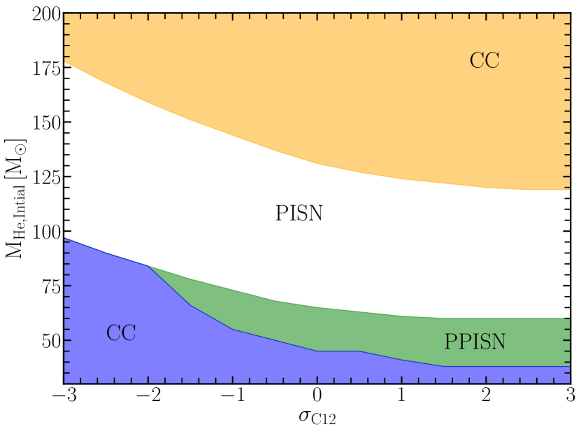
Figure 1: Final fate of a star as function of the initial helium core mass and ${}^{12}\rm{C}\left(\alpha,\gamma\right)^{16}\!\rm{O}$ rate. $\sigma_{\rm{C12}}$ denotes how far the ${}^{12}\rm{C}\left(\alpha,\gamma\right)^{16}\!\rm{O}$ is from the median STARLIB rate, measured in standard deviations. Blue regions indicate stars which undergo core collapse (CC) below the pair instability supernovae (PISN) mass gap, green regions form black holes after a pulsational pair instability supernovae (PPISN), while white regions are completely disrupted in a PISN, and models in the orange region form black holes from core collapse for stars above the PISN mass gap. There are 2210 models, in the grid spaced by $1\,\rm{M}_{\odot}$ and $0.5\sigma_{\rm{C12}}$.

In Fig. 1 we show the outcome for our grid of 2210 evolutionary models as a function of the initial helium core mass and the ${}^{12}\rm{C}\left(\alpha,\gamma\right)^{16}\!\rm{O}$ reaction. We parameterize the ${}^{12}\rm{C}\left(\alpha,\gamma\right)^{16}\!\rm{O}$ in terms of the number of sigmas ($\sigma_{\rm{C12}}$) from the median STARLIB ${}^{12}\rm{C}\left(\alpha,\gamma\right)^{16}\!\rm{O}$ reaction rate:

$$\langle\sigma\nu\rangle=\langle\sigma\nu\rangle_{\rm{median}}e^{\mu\left(T\right)\sigma_{\rm{C12}}}$$ (6)

where $\langle\sigma\nu\rangle_{\rm{median}}$ is the median reaction rate provided by STARLIB, and $\mu\left(T\right)$ is the temperature-dependent uncertainty in the reaction (which is assumed to follow a log-normal distribution).

For higher initial core mass (for a given ${}^{12}\rm{C}\left(\alpha,\gamma\right)^{16}\!\rm{O}$ rate), the final fate of a star transitions from core collapse, to PPISN, to PISN, and then to core collapse again (Bond et al., 1984). As the reaction rate increases (i.e, large values of $\sigma_{\rm{C12}}$) the boundary between the different end fates shifts to lower initial helium core mass. See Section 7 for a discussion of the implications of this for the black hole formation and EM transient rate.

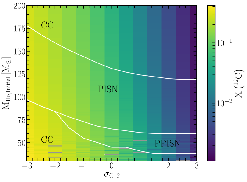
Figure 2: The mass fraction of $\mathrm{{}^{12}C}$ in the core after core helium burning, but before carbon burning, for all initial masses as a function of $\sigma_{\rm{C12}}$. White lines denote the boundaries between the different end fates. Text labels denote the final fate of the star. Grey boxes denote models that do not evolve beyond core helium burning, defined as when the mass fraction of $\mathrm{{}^{4}He}$ at the center of the star drops below $10^{-4}$.

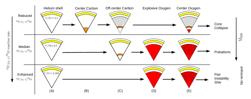
Figure 3: A schematic of the time progression of the major fuel burning, for a star with $\rm{M_{He,init}}=60\,\rm{M}_{\odot}$ as a function of $\sigma_{\rm{C12}}$, at reduced ($\sigma_{\rm{C12}}=-3$), median ($\sigma_{\rm{C12}}=0$), and enhanced ($\sigma_{\rm{C12}}=3$) ${}^{12}\rm{C}\left(\alpha,\gamma\right)^{16}\!\rm{O}$ reaction rates. Yellow regions denote helium burning, orange regions denote carbon burning, and red regions denote oxygen burning. Hatched regions indicate convection mixing regions. Letters match those points marked in Fig. 4. Also shown is the core’s C/O mass ratio at the end of core helium burning.

To understand the reason for these trends, it is insightful to consider the $\mathrm{{}^{12}C}$ mass fraction in the core of the stellar models, after core helium burning has finished. We define the end of core helium burning, when the mass fraction of $\mathrm{{}^{4}He}$ at the center of the star drops below $10^{-4}$. Figure 2 shows that the $\mathrm{{}^{12}C}$ mass fraction in the core of the stars considered here decreases from $\approx 30\%$ to $\approx 0.001\%$ as the ${}^{12}\rm{C}\left(\alpha,\gamma\right)^{16}\!\rm{O}$ rate is increased from $\sigma_{\rm{C12}}=-3$ to $\sigma_{\rm{C12}}=3$, independent of initial mass. This change in the $\mathrm{{}^{12}C}$ mass fraction is what drives the changes in the star’s later phases of evolution and thus final fate.

After core helium burning has ceased the core begins contracting, increasing its density and temperature. However, at the same time, thermal neutrino losses increase which acts to cool the core. The next fuel to burn is, $\mathrm{{}^{12}C}$ via $\mathrm{{}^{12}C}$+$\mathrm{{}^{12}C}$ to $\mathrm{{}^{22}Ne}$, $\mathrm{{}^{23}Na}$, and $\mathrm{{}^{24}Mg}$ (Arnett & Truran, 1969; Farmer et al., 2015). As the $\mathrm{{}^{12}C}+\mathrm{{}^{12}C}$ reaction rate depends on the number density of carbon squared, small changes in the number density of $\mathrm{{}^{12}C}$ can have a large impact on the power generated by the $\mathrm{{}^{12}C}+\mathrm{{}^{12}C}$ reaction.

In Fig. 3 we show a simplified picture of the steps a star takes to its final fate depending on its ${}^{12}\rm{C}\left(\alpha,\gamma\right)^{16}\!\rm{O}$ reaction rate. The top panel shows a star which would undergo core collapse, first by igniting carbon both at the center and then in a off-center shell. This star then avoids igniting oxygen explosively, instead proceeds through its evolution to core collapse. As the ${}^{12}\rm{C}\left(\alpha,\gamma\right)^{16}\!\rm{O}$ increases, the carbon stops igniting at the center and only ignites in a shell (middle panel), before proceeding to ignite oxygen explosively. For the highest ${}^{12}\rm{C}\left(\alpha,\gamma\right)^{16}\!\rm{O}$ shown, no carbon is burnt before oxygen ignites (bottom panel). The C/O ratios shown are defined at the end of core helium burning.

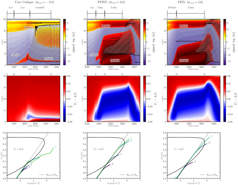
Figure 4: The time evolution of the internal structure of a star for $\rm{M_{He,init}}=60\,\rm{M}_{\odot}$ for different assumptions for the ${}^{12}\rm{C}\left(\alpha,\gamma\right)^{16}\!\rm{O}$ reaction rate. The top row shows the signed logarithm of the net specific power, i.e. $\rm{sign}\left(\epsilon_{\rm{nuc}}-\epsilon_{\nu}\right)\log_{10}\left(\rm{max}\left(1.0,|\epsilon_{\rm{nuc}}-\epsilon_{\nu}|\right)/\left(\rm{erg\,g^{-1}\,s^{-1}}\right)\right)$, where $\epsilon_{\rm{nuc}}$ is the specific power from nuclear reactions and $\epsilon_{\nu}$ is the specific power lost via neutrinos. Purple regions denote strong neutrino cooling and red regions denote regions of strong nuclear burning. Hatched regions indicate convective mixing regions. Text labels state the primary fuel burned in that region. Points marked on the top x axis correspond to those marked in Fig. 3, given with approximate timescales. The middle row shows the evolution of $\Gamma_{1}$ (Equation 1), regions with $\Gamma_{1}-4/3<0$ are locally unstable. The bottom row shows the density-temperature structure of the inner region of the stars at the points marked in the top panel, light colors denote later phases. The dashed line shows where the gas pressure is approximately equal to the radiation pressure. The solid black line that encloses $\Gamma_{1}<4/3$ shows the approximate location of the pair instability region.

Why changing the carbon burning behavior changes the final outcome for a star can be seen in Fig. 4. Here we show the time evolution of the helium cores, for stars with $\rm{M_{He,init}}=60\,\rm{M}_{\odot}$ during carbon burning and up to the ignition of oxygen, for different ${}^{12}\rm{C}\left(\alpha,\gamma\right)^{16}\!\rm{O}$ rates. The top row shows a Kippenhan diagram of the time evolution of the net nuclear energy minus neutrino losses and the mixing regions inside the star. The middle row shows the evolution of $\Gamma_{1}-4/3$. Regions where $\Gamma_{1}-4/3<0$ are locally unstable. The bottom row shows the temperature and density structure inside the star at points in time marked on the top row of Fig. 4. The points in time marked, show how the stars are evolving on different timescales. Timescales vary from a few thermal timescales (left column) to a few dynamical timescales (middle and right columns).

When the ${}^{12}\rm{C}\left(\alpha,\gamma\right)^{16}\!\rm{O}$ rate is small (and thus the $\mathrm{{}^{12}C}$ mass fraction is $\approx 30\%$, with the rest of the core being made of $\mathrm{{}^{16}O}$), $\mathrm{{}^{12}C}$ ignites vigorously at the center in a radiative region (Fig. 4 top-left) and burns outwards until it begins to drive a convective $\mathrm{{}^{12}C}$ burning shell. The star will then ignite oxygen in the core (non-explosively) and proceed through silicon and iron burning before collapsing in a core collapse.

As the ${}^{12}\rm{C}\left(\alpha,\gamma\right)^{16}\!\rm{O}$ rate increases the initial $\mathrm{{}^{12}C}$ ignition point, defined where the nuclear energy generated is greater than the energy lost in neutrinos, moves outwards in mass coordinate (Fig. 4 top-center). As the $\mathrm{{}^{12}C}$ abundance decreases, the star requires a higher density to burn $\mathrm{{}^{12}C}$ vigorously, thus the star must contract further which increases the neutrino losses. No convective carbon shell forms before the oxygen in the core ignites explosively, proceeding to a PPISN. Once the ${}^{12}\rm{C}\left(\alpha,\gamma\right)^{16}\!\rm{O}$ rate increases sufficiently such that the core is depleted in $\mathrm{{}^{12}C}$ after core helium burning, no $\mathrm{{}^{12}C}$ burning region forms and the core proceeds to ignite oxygen explosively (Fig. 4 top-right) as a PISN leaving behind no black hole remnant.

Stars with a convective $\mathrm{{}^{12}C}$ burning shell can resist the collapse caused by the production of $e^{\pm}$, and thus maintain hydrostatic equilibrium until core collapse. Figure 4 (middle-left) shows that when the shell forms it prevents the center of the star from reaching $\Gamma_{1}-4/3<0$. Therefore, the instability is only local and never becomes global: only a small region around the carbon shell becomes unstable. For stars without the convective carbon shell (middle-center and middle-right), a significant fraction of the entire star becomes unstable resulting in a global instability.

Carbon burning begins at the center and moves outwards (either vigorously or not), thus depleting the center of $\mathrm{{}^{12}C}$. Therefore, the carbon shell (if it forms) can not move inwards as there is insufficient fuel for it to burn. The region undergoing carbon burning can not move outwards either, as the convection zone is mixing the energy released from the nuclear reactions over a significant portion of the star. This prevents layers above the carbon burning region from reaching sufficient temperatures and densities needed for vigorous carbon burning (Farmer et al., 2015; Takahashi, 2018).

The convective carbon shell can only be sustained then if it can bring fresh fuel in via convective mixing from the rest of the core. Thus when a convective carbon shell forms it also allows additional fuel to be mixed into the burning region from the outer layers of the core. This prolongs the lifetime of the carbon burning shell and prevents the collapse due to $e^{\pm}$ from occurring, until the carbon shell convective region is depleted in $\mathrm{{}^{12}C}$ which may not occur before the star undergoes core collapse.

As the carbon fraction decreases, the carbon shell burning becomes less energetic (due to the $\mathrm{{}^{12}C}+\mathrm{{}^{12}C}$ reaction depending on the density of carbon squared). Therefore, as $\sigma_{\rm{C12}}{}$ increases (and $\mathrm{{}^{12}C}$ fraction decreases) less energy is released from the carbon burning, thus the fraction of the core where $\Gamma_{1}-4/3<0$ increases There becomes a critical point where the carbon burning is insufficient to prevent the violent ignition of oxygen in the core, thus pulsations begin. Around this critical region, convective carbon burning can still occur, however the burning region can undergo flashes, where the $\mathrm{{}^{12}C}$ ignites but is then quenched. This leads to weaker and shorter lived convection zones which do not mix in sufficient $\mathrm{{}^{12}C}$ to sustain a continuous carbon burning shell. This leads to very weak pulses removing only a few tenths of a solar mass of material. For stars with these weak convection zones the carbon shell only delays the ignition of oxygen; once carbon is sufficiently depleted the oxygen can ignite explosively. Eventually no carbon shell convection zone is formed at all (Fig. 4 middle-center), this leads to larger pulses removing solar masses of material.

The bottom row of Fig. 4 shows the temperature-density profile inside the star at moments marked in the top row of Fig. 4. As the stars evolve the core contracts and heats up, eventually the central regions of the star enter the instability region ($\Gamma_{1}-4/3<0$). Once a convective carbon shell forms (bottom-left) the core stops contracting homogeneously (along the line where the radiation pressure is equal to the gas pressure) and moves to higher densities. This is due to the continued loss of entropy to neutrinos from the core. Thus when oxygen ignites the core is now outside the instability region ($\Gamma_{1}-4/3>0$) and as such does not undergo pulsational mass loss (Takahashi, 2018).

For stars without a convective carbon shell (bottom-center and bottom-right) the core continues to contract homogeneously. When oxygen ignites it does so inside the $\Gamma_{1}-4/3<0$ region. As the temperature increases, due to the oxygen burning, the production of $e^{\pm}$ increases causing a positive feedback loop. This leads to the explosive ignition needed to drive a pulse. Stars undergoing a PPISN (bottom-center) have slightly lower core entropies than stars undergoing a PISN (bottom-right) due to the small amount of non-convective carbon burning that occurs before oxygen burning begins.

Further decreases in the carbon abundance leave little carbon fuel to burn. Thus as the star collapses due to the production of $e^{\pm}$, the oxygen is free to ignite violently. This causes the star to undergo a PISN, completely disrupting the star. This can also be seen in Figure 2 where the boundaries between the different final fates move to lower masses as $\sigma_{\rm{C12}}$ increases, as the pulses become more energetic for a given initial mass.

3.1 Black holes above the PISN mass gap

Figure 1 shows population of black holes that form above the PISN mass gap. These black holes form due to the failure of the PISN explosion to fully unbind the star (e.g., Bond et al., 1984). As the helium core mass is increased (at constant $\sigma_{\rm{C12}}$) a PISN explosion increases in energy, due to a greater fraction of the oxygen being burnt in the oxygen ignition. This increased energy leads to an increase in the maximum core temperature the star reaches, before the inward collapse is reverted and the star becomes unbound. This increased temperature can be seen in the increased production of ${}^{56}\mathrm{Ni}$ as the initial mass increases (Woosley et al., 2002; Renzo et al., 2020a). Eventually the core reaches sufficent temperatures that the energy extracted from the core by photo disintegrations is sufficent to prevent the star from becoming unbound.

Figure 1 shows that as $\sigma_{\rm{C12}}$ increases the initial helium core mass needed to form a black hole above the gap decreases. This is due to the increased production of oxygen as $\sigma_{\rm{C12}}$ increases. At these masses we do not see the formation of a convective carbon shell, even for $\sigma_{\rm{C12}}=-3$, though some radiative carbon burning occurs (similar to point C in the middle panels of Figure 4). Instead the cores with greater total amounts of oxygen can liberate greater amounts of energy from the oxygen burning. This burning raises the temperature in the core, allowing additional nuclosynethesis to occur with the silicon and iron group elements produced from the oxygen burning. For a fixed initial helium core mass as $\sigma_{\rm{C12}}$ increases, the peak core temperature increases. Once a core reaches $\log\ \rm{T/K}\approx 9.86$, then the rate of photodisintegrations is sufficient to prevent the star from unbinding itself. This is what sets the upper edge of the mass gap.

4 Edges of the PISN mass gap

Figure 5 shows the location of the PISN black hole mass gap as a function of the temperature-dependent uncertainty in ${}^{12}\rm{C}\left(\alpha,\gamma\right)^{16}\!\rm{O}$. As the rate increases (with increasing $\sigma_{\rm{C12}}$) both the lower and upper edge of the PISN mass gap shift to lower masses, from $\approx 90\,\rm{M}_{\odot}$ to $\approx 40\,\rm{M}_{\odot}$ for the lower edge and $\approx 175\,\rm{M}_{\odot}$ to $\approx 120\,\rm{M}_{\odot}$ for the upper edge. The width of the region remains approximately constant at $83^{+5}_{-8}\,\rm{M}_{\odot}$. The typical quoted value for the maximum mass of a black hole below the PISN mas gap is $45-55\,\rm{M}_{\odot}$ (Yoshida et al., 2016; Woosley, 2017; Leung et al., 2019; Marchant et al., 2019; Farmer et al., 2019) The gray box in Fig. 5 shows the region of black hole masses, between $\rm{M_{\rm BH}}\approx 90-120\,\rm{M}_{\odot}$, where we can not place a black hole from a first generation core collapse or PPISN model. Thus black holes detected in this mass region would need to come from alternate formation mechanisms, for instance; either second generation mergers (Rodriguez et al., 2016, 2019; Gerosa & Berti, 2019), primordial black holes (Carr et al., 2016; Ali-Haïmoud et al., 2017), or accretion on to the black hole (Di Carlo et al., 2020a; Roupas & Kazanas, 2019; van Son et al., 2020).

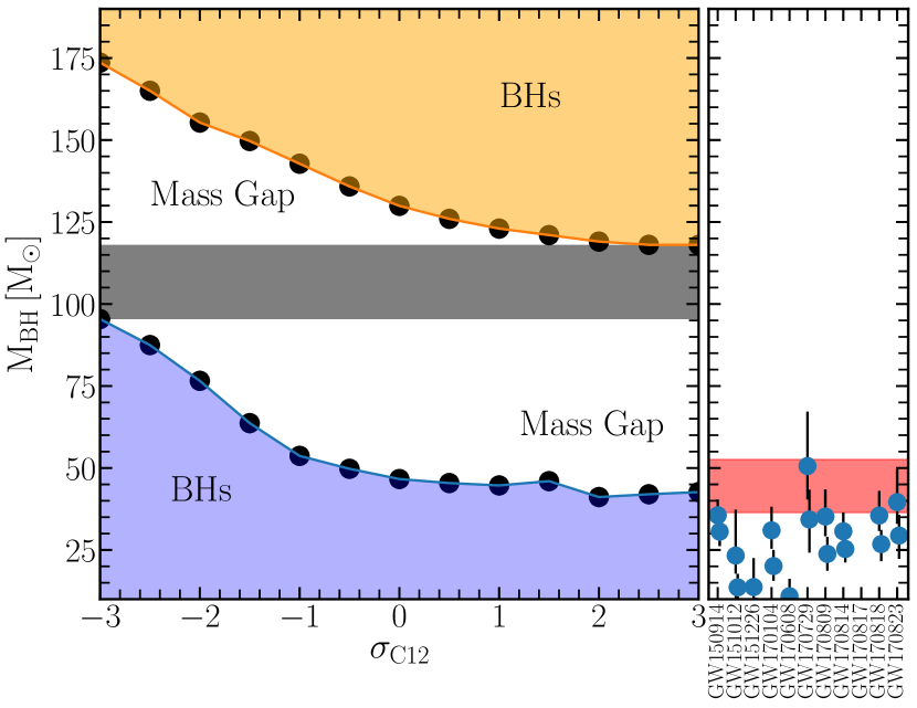
Figure 5: The location of the PISN mass gap as a function of the temperature-dependent uncertainty in the ${}^{12}\rm{C}\left(\alpha,\gamma\right)^{16}\!\rm{O}$ reaction rate. The white region denotes the mass gap, while the grey horizontal bar region denotes the mass range where we can not place a black hole for any value of the ${}^{12}\rm{C}\left(\alpha,\gamma\right)^{16}\!\rm{O}$ rate. The side plot shows the inferred masses of the currently known black holes from LIGO/Virgo O2 (Abbott et al., 2019a), with their 90% confidence intervals. The red region shows the 90% confidence range for the inferred location of the lower edge of the PISN mass gap from the O1/O2 data (Abbott et al., 2019b).

The detection of the upper edge of the PISN mass gap ($\rm{M_{\rm BH}}>120\,\rm{M}_{\odot}$) would provide a strong constraint on the ${}^{12}\rm{C}\left(\alpha,\gamma\right)^{16}\!\rm{O}$ rate. This edge has smaller numerical uncertainties associated with it, as it is defined only by a combination of fundamental physics (nuclear reaction rates and the equation of state of an ionized gas) and does not depend on the complexities of modeling the hydrodynamical pulses which define the lower edge of the PISN mass gap. Mergers in this mass range are expected to be rare due to the difficulty in producing sufficiently massive stars in close binaries (Belczynski et al., 2016b), however they may be detectable by third generation gravitational wave detectors (Mangiagli et al., 2019).

4.1 Other sources of the ${}^{12}\rm{C}\left(\alpha,\gamma\right)^{16}\!\rm{O}$ rate

Table 1 shows the maximum black hole mass as a function of different sources for the ${}^{12}\rm{C}\left(\alpha,\gamma\right)^{16}\!\rm{O}$ reaction. The Sallaska et al. (2013) STARLIB rate is based on that of Kunz et al. (2002), however STARLIB assumes rate probability density is lognormal thus its median value is $\sqrt{\rm{R_{Low}}\times\rm{R_{High}}}$ (eqaution 17 Sallaska et al. (2013)), where $\rm{R_{Low}}$ and $\rm{R_{High}}$ are from Kunz et al. (2002). The maximum black mass for the deBoer et al. (2017) rate is computed using the “adopted”, “lower”, and “upper” rates from Table XXV of deBoer et al. (2017). The lower edge of the black hole mass gap over the different sources is between $47-51\,\rm{M}_{\odot}$, with an uncertainty on the maximum black hole mass of $<5\%$. The upper edge varies between $130-136\,\rm{M}_{\odot}$, with a similar uncertainty on the maximum black hole mass of $<5\%$.

The small variations seen in the edges of the PISN mass gap, are due to the fact that the different sources of the ${}^{12}\rm{C}\left(\alpha,\gamma\right)^{16}\!\rm{O}$ have been slowly converging over time on a S-factor between $140-160\rm{\,\mathrm{keV}\,barns}$ (See figure 7). See Figure 26 of deBoer et al. (2017) for a review of how the uncertainty in the different energy levels has improved since the 1970’s.

Table 1: Location of the edges of the PISN mass gap for different sources of the ${}^{12}\rm{C}\left(\alpha,\gamma\right)^{16}\!\rm{O}$ reaction rate. Uncertainties quoted are $1\sigma$ where applicable.

Source	Lower [$\,\rm{M}_{\odot}$]	Upper [$\,\rm{M}_{\odot}$]
$1.7\times$ Caughlan & Fowler (1988)	49	135
Angulo et al. (1999) (NACRE)	49	130
Kunz et al. (2002)	50	134
Cyburt et al. (2010) (REACLIB)	50	136
Sallaska et al. (2013) (STARLIB)	$47^{+7}_{-2}$	$130^{+13}_{-7}$
deBoer et al. (2017)	$51^{+0}_{-4}$	$134^{+5}_{-5}$

Table 2: The relative change in the location of the upper and lower edge of the PISN mass gap, when varying both the ${}^{12}\rm{C}\left(\alpha,\gamma\right)^{16}\!\rm{O}$ reaction rate and either the $3\alpha$, $\mathrm{{}^{12}C}$+$\mathrm{{}^{12}C}$, or $\mathrm{{}^{16}O}$+$\mathrm{{}^{16}O}$ reaction rate, with respect to our default choices.

Rate	Uncertainty	${}^{12}\rm{C}\left(\alpha,\gamma\right)^{16}\!\rm{O}$
		$\sigma_{\rm{C12}}=-3$		$\sigma_{\rm{C12}}=0$		$\sigma_{\rm{C12}}=+3$
		Lower	Upper	Lower	Upper	Lower	Upper
$3\alpha$	$+1\sigma$	0$-1.0\%$	0$-2.7\%$	+0$1.7\%$	0$-0.8\%$	0$-4.3\%$	0$-0.8\%$
Sallaska et al. (2013)	$-1\sigma$	+0$6.2\%$	+0$4.2\%$	+0$8.9\%$	+0$4.6\%$	0$-7.6\%$	+0$0.8\%$
$\mathrm{{}^{12}C}+\mathrm{{}^{12}C}$	$+1\sigma$	0$-1.0\%$	+0$0.5\%$	+$16.6\%$	+$\sim 0.0\%$	0$-16.8\%$	+$\sim 0.0\%$
Tumino et al. (2018)	$-1\sigma$	+0$1.9\%$	+0$0.5\%$	0$-1.4\%$	+$\sim 0.0\%$	0$-1.2\%$	+$\sim 0.0\%$
$\mathrm{{}^{16}O}+\mathrm{{}^{16}O}$	$\times 10$	+0$0.0\%$	0$-1.8\%$	00$0.0\%$	0$-2.3\%$	0$-2.6\%$	0$-3.3\%$
Caughlan & Fowler (1988)	$\times 0.1$	+0$0.0\%$	+0$4.4\%$	+0$5.7\%$	+0$9.1\%$	+0$6.9\%$	+0$9.2\%$

4.2 Sensitivity to other reaction rates

Table 2 shows how the maximum black hole mass varies as a function of both the ${}^{12}\rm{C}\left(\alpha,\gamma\right)^{16}\!\rm{O}$ rate and other reaction rates that either create carbon (the $3\alpha$ reaction), destroy carbon ($\mathrm{{}^{12}C}+\mathrm{{}^{12}C}$), and oxygen burning ($\mathrm{{}^{16}O}+\mathrm{{}^{16}O}$). For each rate varied we compute the location of the mass gap for the number of standard deviations from the median for that rate, and for variations in the ${}^{12}\rm{C}\left(\alpha,\gamma\right)^{16}\!\rm{O}$ reaction. This is to probe for correlations between the rates. In the case of the rates from Caughlan & Fowler (1988) we follow the uncertainty provided by STARLIB and we multiply (divide) the rate by a fixed factor of 10 due to the lack of knowledge of the uncertainty in this rate. Table 2 then shows the fractional change in the location of each edge of the mass gap, as an indication of how sensitive the edges of the mass gap are to other uncertainties. In general the maximum fractional error is $\approx 5-15\%$ from considering other reactions, in the location of the PISN mass gap.

We would expect that varying a rate between its upper and lower limits would produce relative changes with opposing signs, however in some cases this does not occur. This is due to numerical difficulties in the evolution of the models. Some of these models would fail to reach core collapse, and thus we could not measure the peak of the black hole mass distribution. Instead, we report the largest black hole mass only for the models that successfully reach core collapse. This means that the relative change we measure includes changes in the initial mass as well as the black hole mass. Table 2 should therefore be taken as a representation of the changes expected for different rates, but it does not show the complete picture.

For the STARLIB median ${}^{12}\rm{C}\left(\alpha,\gamma\right)^{16}\!\rm{O}$ reaction rate, the $3\alpha$ reaction produces a fractional uncertainty of $1-10\%$, independent of the ${}^{12}\rm{C}\left(\alpha,\gamma\right)^{16}\!\rm{O}$ rate. By increasing the $3\alpha$, within its one sigma uncertainties, rate we decrease the maximum black hole mass. There is a much larger change when reducing the rate than when the rate is increased.

To test variations in the $\mathrm{{}^{12}C}+\mathrm{{}^{12}C}$ we use the rate provided by Tumino et al. (2018), which provides a temperature dependent $1\sigma$ uncertainty on the reaction rate. However, the uncertainty is only available up to $3\,\rm{GK}$, at higher temperatures we revert to MESA’s standard $\mathrm{{}^{12}C}+\mathrm{{}^{12}C}$ reaction rate, which does not have a provided uncertainty estimate (Caughlan & Fowler, 1988).

It is difficult to determine the trend in black hole mass compared to the $\mathrm{{}^{12}C}+\mathrm{{}^{12}C}$ given a number of models due not converge. We might expect variations around $\approx 15\%$. The larger change occurs when the $\sigma_{\rm{C12}}\geq 0$ than when $\sigma_{\rm{C12}}=-3$. This is due to the change in the power generated during the carbon burning. When the $\mathrm{{}^{12}C}+\mathrm{{}^{12}C}$ rate is increased then stars with low $\mathrm{{}^{12}C}$ fractions ($\sigma_{\rm{C12}}\geq 0$), which would not generate a convective carbon shell (when $\mathrm{{}^{12}C}+\mathrm{{}^{12}C}$ is small) can now generate sufficient power to alter the core structure and potentially drive the formation of convective carbon burning shell. See however Tan et al. (2020) for a discussion on why the Tumino et al. (2018) rate may have been overestimated, and Fruet et al. (2020) for a discussion on new measurement techniques of the $\mathrm{{}^{12}C}+\mathrm{{}^{12}C}$ rate.

As the $\mathrm{{}^{16}O}+\mathrm{{}^{16}O}$ rate increases the maximum black hole mass decreases. This change is asymmetric, with a larger change occurring when the rate decreases than when the rate increases. The 0% change seen when $\sigma_{\rm{C12}}=-3$, is due to those stars lacking pulsations. As the star has a high $\mathrm{{}^{12}C}$ fraction, and thus a carbon shell, it does not undergo explosive oxygen burning only stable core oxygen burning. As there are no pulsations no mass is lost. This rate does have an effect on the core structure of the star, which might lead to variations in the mass lost during the final collapse into a black hole. For larger values of $\sigma_{\rm{C12}}$ there is up to a $10\%$ variation in the location of the edges of the PISN mass gap.

More work is needed to understand the correlations between the different reaction rates and their effect on our ability to constrain the edges of the PISN mass gap, e.g. West et al. (2013). We need to improve our understanding of how the uncertainty in the rates at different temperatures alters the behavior of the carbon shell and the final black hole mass. This could be achieved with a Monto-Carlo sampling of the reactions rates, e.g. Rauscher et al. (2016); Fields et al. (2016, 2018), however this comes at a much greater computational cost.

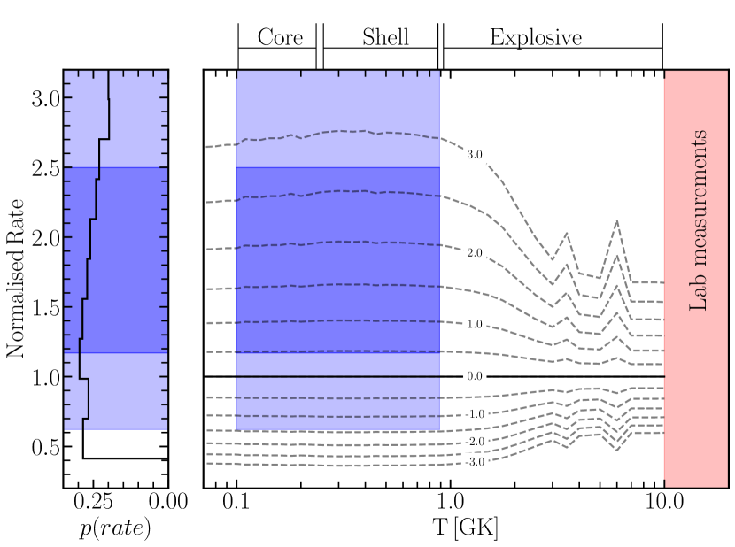
Figure 6: The right pannel shows the ${}^{12}\rm{C}\left(\alpha,\gamma\right)^{16}\!\rm{O}$ rate as a function of temperature, normalized to the median STARLIB rate $\langle\sigma\nu\rangle/\langle\sigma\nu\rangle_{\rm{median}}=e^{\mu\left(T\right)\sigma_{\rm{C12}}}$. The left panel shows the posterior of our distribution. The solid line, labeled 0.0, indicates the normalized median rate (i.e., $\sigma_{\rm{C12}}$=0.0). The dashed lines show the reaction rates above and below the median STARLIB rate, labeled by the appropriate value of $\sigma_{\rm{C12}}$. We assume that the black hole mass distribution is given by model B of Abbott et al. (2019b). The dark blue region shows the 50% confidence range in the ${}^{12}\rm{C}\left(\alpha,\gamma\right)^{16}\!\rm{O}$ rate, while the lighter blue shows the 90% confidence interval. Note the upper rate limit is unbounded when adopting the current O2 LIGO/Virgo posteriors on the maximum black hole mass. The red region ($\rm{T}>10\,GK$) shows the approximate lower edge of the energy range for lab measurements of the ${}^{12}\rm{C}\left(\alpha,\gamma\right)^{16}\!\rm{O}$ rate (Holt et al., 2019).

5 Constraining the ${}^{12}\rm{C}\left(\alpha,\gamma\right)^{16}\!\rm{O}$ reaction rate with gravitational waves

Because of the sensitivity of the edges of the PISN mass gap to the ${}^{12}\rm{C}\left(\alpha,\gamma\right)^{16}\!\rm{O}$ reaction rate, we can use the measured location of the gap to derive a value for the ${}^{12}\rm{C}\left(\alpha,\gamma\right)^{16}\!\rm{O}$ at astrophysically relevant temperatures. See Appendix B for the sensitivity of our results to different temperature ranges. We focus here on the lower edge of the mass gap, as it has been inferred from the existing LIGO/Virgo data (Abbott et al., 2019b).

The currently most massive black hole in O1/O2, as inferred by LIGO/Virgo is GW170729 at $\rm{M_{\rm BH}}=50.6^{+16.6}_{-10.2}\,\,\rm{M}_{\odot}$ (Abbott et al., 2019b), which could be used as an estimate for the location of the PISN mass gap, assuming that it is from a first generation black hole. There are also several other candidates for the most massive black hole. This includes IMBHC-170502 has which has been inferred to have individual black hole components with masses $\approx 94\,\rm{M}_{\odot}$ and $\approx 62\,\rm{M}_{\odot}$ (Udall et al., 2019). GW151205 has also been proposed to have one component with an inferred mass of $\rm{M_{\rm BH}}=68^{+28}_{-17}\,\rm{M}_{\odot}$ (Nitz et al., 2020). By having a component mass inside the classical PISN mass gap it was suggested that this was the result of dynamical mergers.

However, we must be careful in not over-interpreting single events, which may be susceptible to noise fluctuations (Fishbach et al., 2020) which can make a black hole have a higher apparent mass than it truly does. For instance, considering GW170729 jointly with the other O1/O2 detections, lowers its mass to $\rm{M_{\rm BH}}=38.9^{+7.3}_{-4.5}\,\rm{M}_{\odot}$, which places it below the PISN mass gap.

Thus we must consider the entire population of binary black hole mergers as a whole, when measuring the maximum inferred black hole mass below the gap. The 10 detections in O1/O2 places the maximum black hole mass below the PISN mass gap at $42-44\,\rm{M}_{\odot}$ depending on the choice of model parameters (Abbott et al., 2019b). The current 90% confidence interval on this value is $\approx\pm 10\,\rm{M}_{\odot}$. With a large enough population ($\mathcal{O}(50)$) of black holes we can place limits of $\approx\pm 1\,\rm{M}_{\odot}$ on the location of the gap (Fishbach & Holz, 2017; Abbott et al., 2019b).

We assume that all binary black hole mergers so far detected come from isolated binaries or first generation black hole mergers, thus the maximum mass black holes below the gap come from PPISN. We also assume that only uncertainties in ${}^{12}\rm{C}\left(\alpha,\gamma\right)^{16}\!\rm{O}$ matter. Thus we can use the posterior distribution over the maximum black hole mass for the population of black holes as the estimate of the maximum black hole mass below the mass gap.

Figure 6 shows the uncertainty in the STARLIB ${}^{12}\rm{C}\left(\alpha,\gamma\right)^{16}\!\rm{O}$ reaction rate as a function of temperature. Over the temperatures we are sensitive to, less than $1.0\,\rm{GK}$ where helium burns non-explosively, the uncertainty is approximately constant. Thus we need only find a single temperature-independent $\sigma_{\rm{C12}}$ to fit to the maximum black hole mass below the gap.

We fit a 4^th order polynomial to the lower edge of the PISN mass gap (Fig. 5) to map from maximum black hole mass to $\sigma_{\rm{C12}}$. This is then combined with the posterior of the maximum black hole mass to generate a posterior distribution over $\sigma_{\rm{C12}}$. The blue boxes in Fig. 6 show our 50% and 90% confidence interval on $\sigma_{\rm{C12}}$. At 50% confidence, we can limit $\sigma_{\rm{C12}}$ to be between 0.5 and 2.5$\sigma_{\rm{C12}}$, while at 90% confidence we can only place a lower limit of $\sigma_{\rm{C12}}>-1.5$. This is due to the posterior distribution from LIGO/Virgo allowing the maximum black hole mass to be $\rm{M}_{\rm{BH,max}}<40\,\rm{M}_{\odot}$, which is below the lower limit we find for the edge of the mass gap.

By taking the STARLIB astrophysical S-factor, at $300\mathrm{keV}$, to be $165\rm{\,\mathrm{keV}\,barns}$ (Sallaska et al., 2013) we can scale the S-factor from the $\sigma_{\rm{C12}}$. As the normalized rate is approximately flat (Fig. 6) the uncertainty is flat. Using Equation 4 and Fig. 6 we have $e^{\mu\left(T\right)\sigma_{\rm{C12}}}=\langle\sigma\nu\rangle/\langle\sigma\nu\rangle_{\rm{median}}\propto S(300\,\mathrm{keV})$ , thus the S-factor can be linearly scaled from its STARLIB value to a new value, given by a different $\sigma_{\rm{C12}}$.

Figure 7 shows a comparison between the values for the S-factor from nuclear laboratory experiments, constraints placed by white dwarf asterosiesmology and galactic chemical enrichment models, and this study. For our assumptions we find the S-factor for the ${}^{12}\rm{C}\left(\alpha,\gamma\right)^{16}\!\rm{O}$ rate at $300\mathrm{keV}$ to be $S_{300}>175\rm{\,\mathrm{keV}\,barns}$, at 68% confidence. At 95% confidence we find a limit of $S_{300}>82\rm{\,\mathrm{keV}\,barns}$ and at 99% confidence we find a limit of $S_{300}>68\rm{\,\mathrm{keV}\,barns}$. The S-factors computed here are consistent with experimentally derived values, though we only currently place a lower limit on the S-factor. See section 6 for a discussion on how this limit may be improved with future gravitational wave detections. Figure 7 also shows the lower limit on the S-factor if PPISN can be shown to exist though other means, for instance electromagnetic observations of the SN. The existence of PPISN would imply that $S_{300}>79\rm{\,\mathrm{keV}\,barns}$, this is discussed further in Section 7.2.

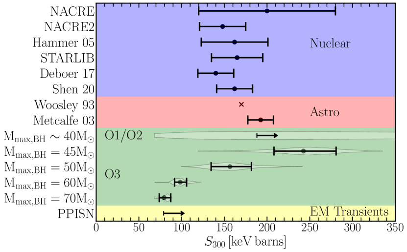
Figure 7: Constraints on the S-factor at $300\mathrm{keV}$ for the ${}^{12}\rm{C}\left(\alpha,\gamma\right)^{16}\!\rm{O}$ reaction rate. The blue region presents values for commonly-used nuclear reaction rate libraries, while the red region shows values inferred from astrophysical measurements, by observations of white dwarfs (Metcalfe, 2003) and from the galactic chemical enrichment model of Woosley et al. (1993). The green region show our posteriors on the ${}^{12}\rm{C}\left(\alpha,\gamma\right)^{16}\!\rm{O}$ derived from the O1/O2 maximum black hole mass inferred from model B of Abbott et al. (2019b), and for 50 simulated binary black-hole observations, approximately the number expected in O3, assuming that the O3 detections follow the power law model B from Abbott et al. (2019b). Error bars show the 68% confidence intervals on our inferred S-factor at $300\mathrm{keV}$. The yellow region shows the constraints placed if PPISN supernovae exist (Section 7.2). Error bars in the blue and red regions are $1\sigma$ uncertainties. We assume that the uncertainty from Shen et al. (2020) is the same as that of deBoer et al. (2017).

5.1 GW190521

The detection of GW190521 (Abbott et al., 2020a) with component masses of $85^{+21}_{-14}\,\rm{M}_{\odot}$ and $66^{+17}_{-18}\,\rm{M}_{\odot}$ places both black holes firmly in the mass gap, as inferred from the O1/O2 observations (Abbott et al., 2020b). However, if we assume that the primary black hole in GW190521 was a first generation black hole, this leads to an inference of $\sigma_{\rm{C12}}=-2.4^{+0.6}$, and thus $S(300\,\mathrm{keV})=73^{+11}\rm{\,\mathrm{keV}\,barns}$. We can not infer a lower limit as the 90% confidence interval for the mass extends above $\rm{M_{\rm BH}}\approx 95\,\rm{M}_{\odot}$ where our models can not place a black hole, below the mass gap. If $\sigma_{\rm{C12}}\approx-2.5$, then PPISN would be suppressed due to the carbon burning shell. Instead, if we assume that only the secondary object was a first generation black hole we would infer a $\sigma_{\rm{C12}}=-1.7^{+1.8}_{-0.5}$, and thus $S(300\,\mathrm{keV})=87^{+84}_{-12}\rm{\,\mathrm{keV}\,barns}$.

However, it is unlikely that GW190521 is a pair of first generation black holes, instead it is likely to be a pair of second generation black holes, perhaps inside an AGN disk (Abbott et al., 2020b). Indeed, (Graham et al., 2020) claims a tentative detection of EM counterpart (ZTF19abanrhr) due to the merger product ramming into an AGN disk. However, the redshift of the AGN does not agree with the GW-inferred redshift. Further investigation of this event and the likelihood of a double second generation merger in an AGN disk is warranted. The presence of black holes in the expected mass gap region can make the analysis of the location of the gap more difficult, though folding in a prior based on the ${}^{12}\rm{C}\left(\alpha,\gamma\right)^{16}\!\rm{O}$ may help to identify outliers that have formed through alternative formation mechanisms.

6 Prospects for constraining ${}^{12}\rm{C}\left(\alpha,\gamma\right)^{16}\!\rm{O}$ from future GW detections

With the release of the O3 data from LIGO/Virgo, it is predicted that there will be $\mathcal{O}(50)$ BBH detections (Abbott et al., 2018). Thus we can ask how well can we expect to do with additional observations? This depends strongly on what value the lower edge of the PISN mass gap is found to be.

We assume that the detections in O3 will follow a power law in primary mass ($\rm{M}_{1}$) of the black hole in the binary, with the form previously assumed for the O1/O2 data (Abbott et al., 2019b). Thus we have:

$$p(\rm{M}_{1})\propto\rm{M}_{1}^{\alpha}$$ (7)

for $\rm{M_{min}}<\rm{M}_{1}<\rm{M_{max}}$, where $\rm{M_{min}}$ is the minimum possible black hole mass below the PISN mass gap, and $\rm{M_{max}}$ is the maximum possible black hole mass. We also assume that the secondary mass $\rm{M_{2}}$ follows:

$$p(\rm{M}_{2}|\rm{M}_{1})\propto\rm{M}_{2}^{\beta}$$ (8)

where $\rm{M_{min}}<\rm{M}_{2}<\rm{M}_{1}$. This is equivalent to model B of Abbott et al. (2019b). We set $\rm{M_{min}}=5\,\rm{M}_{\odot}$ and $\beta=4$ to be consistent with the current O1/O2 observations (Abbott et al., 2019b). There is a strong correlation between the values of $\alpha$ and $\rm{M_{max}}$. Thus for different choices of $\rm{M_{max}}$ we choose a value of $\alpha$ that remains consistent with the O1/O2 data (e.g, Fig. 3 of Abbott et al. (2019b)). As $\rm{M_{max}}$ increases, we require a larger $\alpha$ value. We consider 4 possible locations for the lower edge of the PISN mass gap ($\rm{M_{max}}$) to explore how the uncertainty both from the LIGO/Virgo measurements and from our stellar models affects our determination of the ${}^{12}\rm{C}\left(\alpha,\gamma\right)^{16}\!\rm{O}$ rate. We considered $\rm{M_{max}}=45,50,60,70\,\rm{M}_{\odot}$, and we choose $\alpha=-1.5,-1.5,-2,-3$, to remain consistent with the joint $\alpha,\rm{M_{max}}$ posterior from O1/O2 (Abbott et al., 2019b).

We generate 50 mock detections from each of the four mass distributions described above. We assume that the underlying merger rate density is constant in redshift, and that sources are detected if they pass an SNR threshold of 8 in a single detector. We neglect the spins of the black holes in this study, as the maximum mass is well-measured independently of the underlying spin distribution. For each mock detection, we simulate the measurement uncertainty on the source-frame masses according to the prescription in Fishbach et al. (2020), which is calibrated to the simulation study of Vitale et al. (2017). This gives a typical $1\sigma$ measurement uncertainty of $\sim 30\%$ on the source-frame masses. We then perform a hierarchical Bayesian analysis (Mandel, 2010; Mandel et al., 2019) on each set of 50 detections to recover the posterior over the population parameters, $\alpha$, $M_{\mathrm{max}}$, $\beta$ and $M_{\mathrm{min}}$. This provides a projection of how well $M_{\mathrm{max}}$, the maximum mass below the PISN mass gap, can be measured with 50 observations. We sample from the hierarchical Bayesian likelihood using PyMC3 (Salvatier et al., 2016). Finally, we translate the projected measurement of $M_{\mathrm{max}}$ under each of the simulated populations to a measurement of the ${}^{12}\rm{C}\left(\alpha,\gamma\right)^{16}\!\rm{O}$ reaction rate according to Fig. 5.

Figure 7 shows our inferred S-factors (at $300\mathrm{keV}$) for different choices of the maximum black hole mass below the PISN mass gap. As the maximum black hole mass increases, the S-factor decreases (as stars have more $\mathrm{{}^{12}C}$ in their core and thus have reduced mass loss from pulsations). The 68% confidence interval also reduces in size as the maximum black hole mass increases. The predicted accuracy with which LIGO/Virgo is expected to infer the maximum black hole mass decreases as the mass increases, as we require a steeper power law index $\alpha$ to be consistent with the O1/O2 observations. This leads to fewer mergers near the gap. However, the maximum black hole mass becomes more sensitive to the choice of $\sigma_{\rm{C12}}$. This can be seen in the gradient of the lower edge of the PISN mass gap in Fig. 5, which increases as $\sigma_{\rm{C12}}$ decreases. We caution that we have likely under-estimated the size of the uncertainty range, especially at the higher black hole masses, due to the effect of uncertainties in other reaction rates and mass lost during the formation of the black hole. With the predicted accuracy expected for LIGO/Virgo during O3 in inferring the maximum black hole mass, we will be limited by the accuracy of our models, not the data, in constraining the ${}^{12}\rm{C}\left(\alpha,\gamma\right)^{16}\!\rm{O}$ reaction rate.

7 Other observables

7.1 Formation rates

Given that the initial mass function (IMF) strongly favors less massive progenitors, this would imply that PPISN and PISN would be more common at higher values of $\sigma_{\rm{C12}}$ (higher ${}^{12}\rm{C}\left(\alpha,\gamma\right)^{16}\!\rm{O}$ rates), all else being equal. This is potentially detectable given a sufficiently large population of binary black hole mergers or PPISN/PISN transients, and could provide additional constraints on the ${}^{12}\rm{C}\left(\alpha,\gamma\right)^{16}\!\rm{O}$ rate. A number of upcoming surveys, including LSST, JWST, and WFIRST, are expected to find significant numbers of PPISN and PISN transients (Young et al., 2008; Hummel et al., 2012; Whalen et al., 2013a, b; Villar et al., 2018; Regős et al., 2020).

To provide a rough estimate for this, we make the simplified assumption that the helium core masses follow a Salpeter-like IMF with a power law $\alpha=-2.35$, so that we can compare the relative difference in formation rates for stars with $\sigma_{\rm{C12}}=\pm 1$. We take the smallest helium cores to be $\rm{M_{He,init}}=30\,\rm{M}_{\odot}$ (the least massive stars modeled in our grid), and the maximum helium core mass that makes a black hole as: $73\,\rm{M}_{\odot}$ for $\sigma_{\rm{C12}}=-1$, and $61\,\rm{M}_{\odot}$ for $\sigma_{\rm{C12}}=+1$. This folds together the formation rates of black holes from both core collapse and PPISN, as gravitional waves can not distinguish these objects from their gravitional wave signal alone. This leads to a relative increase in the formation rates of black holes of $\approx 10\%$ for the $\sigma_{\rm{C12}}=-1$ over $\sigma_{\rm{C12}}=+1$ models. There is a larger variation possible, if we consider how the lowest-mass helium core that makes a black hole varies with ${}^{12}\rm{C}\left(\alpha,\gamma\right)^{16}\!\rm{O}$. For $\sigma_{\rm{C12}}=\pm 1$ this puts the lower limit at $5\,\rm{M}_{\odot}$ and $8\,\rm{M}_{\odot}$ (Sukhbold & Adams, 2020), which would lead to a factor 2 difference in the formation rates of black holes. This is mostly due to the change in the relative number of low mass black holes.

Figure 8 shows the black hole masses as a function of the initial helium core mass, for different choices of $\sigma_{\rm{C12}}$. At the lowest values of $\sigma_{\rm{C12}}$, no star undergoes PPISN, thus the black hole mass scales lineraly with the initial helium core mass. As $\sigma_{\rm{C12}}$ increases the final black hole mass shifts to lower masses away from a linear relationship with the helium core mass, due to pulsational mass loss. There is also a turn over in the initial-black hole mass realtionship, where the most massive black holes do not form from the most massive stars undergoing PPISN (Farmer et al., 2019). This turn over may be detectable in the infered black hole mass distribution (see model C of Abbott et al. 2019b). There may also be a small bump in the black hole mass distribution at the interface between the stars undergoing CC and the lightest PPISN progenitors, depending on the strength of the mass loss in the lighest PPISN progenitors (Renzo et al., 2020b). We chose not to show Figure 8 in terms of the carbon core mass, which is the more applicable quantity to show when comparing between different metalicities (Farmer et al., 2019), as the highest $\sigma_{\rm{C12}}$ models have $X\left({}^{12}\rm{C}\right)\approx 0$ in their cores. This leads to the carbon core mass being ill-defined.

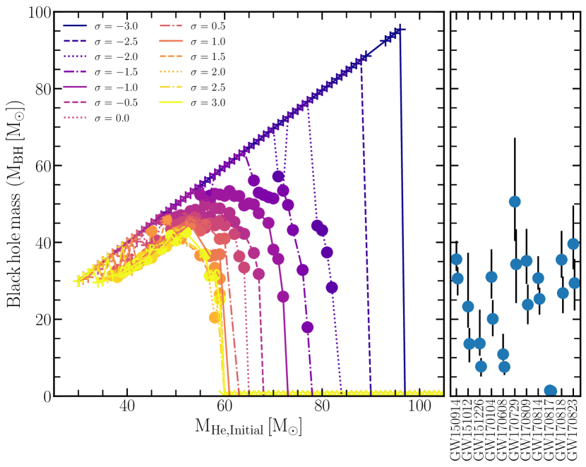
Figure 8: The final black hole mass as a function of the initial helium core mass. The colors represent different choices for $\sigma_{\rm{C12}}$. Circles denote models which undergo pulsational mass loss (PPISN) while plus symbols denote models which do not undergo mass lost due to pulsations (CC). The right pannel shows the inferred masses of the currently known black holes from LIGO/Virgo O2 (Abbott et al., 2019a), with their 90% confidence intervals.

We can compare the formation rates of PPISN (and thus potentially detectable supernovae) only for $\sigma_{\rm{C12}}>-2.0$. As an indication of the variation, we consider the relative change (due to the IMF) in formation rates only for $\sigma_{\rm{C12}}{}=\pm 1$. We find the helium core masses for stars that we would classify as undergoing a PPISN, as $41-61\,\rm{M}_{\odot}$ for $\sigma_{\rm{C12}}=+1$, and $55-73\,\rm{M}_{\odot}$ for $\sigma_{\rm{C12}}=-1$. This leads to a increase by a factor of 2 for $\sigma_{\rm{C12}}=+1$ over $\sigma_{\rm{C12}}=-1$. However, there can be difficulty in determining which stars are PPISN due to the small amounts of mass lost for the lightest PPISN progenitors (Renzo et al., 2020a).

For the rate of PISN, we find the initial helium core masses to be $61-124\,\rm{M}_{\odot}$ for $+1\sigma_{\rm{C12}}$, and $73-142\,\rm{M}_{\odot}$ for $\sigma_{\rm{C12}}=-1$, These ranges then lead to a relative increase of $\approx 30\%$ for the rate of PISN for $\sigma_{\rm{C12}}=+1$ compared to $\sigma_{\rm{C12}}=-1$. These variations are driven by the change in the lower masses needed for a PPISN or PISN as the ${}^{12}\rm{C}\left(\alpha,\gamma\right)^{16}\!\rm{O}$ rate increases (Takahashi, 2018).

7.2 Observations of supernovae

In Fig. 1 we show that when $\sigma_{\rm{C12}}<-2$ no PPISN are formed. This provides an intriguing observational test for the ${}^{12}\rm{C}\left(\alpha,\gamma\right)^{16}\!\rm{O}$ reaction rate. If the existence of PPISN can be confirmed though photometric observations (for instance candidate PPISN SN2006gy (Woosley et al., 2007), SN2006jc (Pastorello et al., 2007), SN iPTF14hls (Arcavi et al., 2017; Woosley, 2018; Vigna-Gómez et al., 2019), SN iPTF16eh (Lunnan et al., 2018), or SN2016iet (Gomez et al., 2019), or SN2016aps (Nicholl et al., 2020)) then we can place a lower limit on the ${}^{12}\rm{C}\left(\alpha,\gamma\right)^{16}\!\rm{O}$ reaction rate of $\sigma_{\rm{C12}}>-2.0$.

The outer layers of the star that are expelled in a pulsational mass loss event, or even the small amount of material that might be ejected in the final collapse to a black hole, provides some information on the final composition of the star, though this will depend on the star’s metallicity and assumed wind mass loss rate. In general the lowest mass stars that undergo a PPISN, in our grid, have surface layers dominated by $\mathrm{{}^{4}He}$, while the higher mass stars have $\mathrm{{}^{16}O}$ rich outer layers (Renzo et al., 2020a).

As the initial mass increases, and the pulses get stronger and thus remove more mass they can expose $\mathrm{{}^{16}O}$ rich layers, with traces of $\mathrm{{}^{20}Ne}$, $\mathrm{{}^{23}Na}$, $\mathrm{{}^{24}Mg}$, and $\mathrm{{}^{28}Si}$ (Renzo et al., 2020a). However, the $\mathrm{{}^{12}C}$ fraction in the outer layers follows the same trend seen in the core $\mathrm{{}^{12}C}$ fraction. As the ${}^{12}\rm{C}\left(\alpha,\gamma\right)^{16}\!\rm{O}$ reaction rate increases more $\mathrm{{}^{12}C}$ is converted into $\mathrm{{}^{16}O}$ in helium shell burning. Therefore, the measured abundances could provide additional constraints on ${}^{12}\rm{C}\left(\alpha,\gamma\right)^{16}\!\rm{O}$, and may provide constraints in a reduced temperature region (that associated with shell helium burning, $0.3<\rm{T}/\,\rm{GK}<1.0$). Further work is needed to quantify the amount of mixing in the outer layers of the star (Renzo et al., 2020b), understanding which parts of the ejecta (and thus which layers of the star) would be measured in spectroscopy of a PPISN (Renzo et al., 2020a), as well as investigating the effect of a larger nuclear network to follow in greater detail the nucleosynthetic yields from the explosive oxygen burning (Weaver & Woosley, 1993; Heger & Woosley, 2002; Woosley & Heger, 2007; West et al., 2013).

8 Discussion

This work assumes that all black holes found by LIGO/Virgo so far have come from stars that lose their hydrogen envelope before their collapse to a black hole. Thus the maximum mass a black hole can have is limited by PISN and mass loss from PPISN. However there are formation mechanisms which may place a black hole in the mass gap. If a star can retain its hydrogen envelope until collapse, though a combination of weak stellar winds (Woosley, 2017) or for a stellar merger (Vigna-Gómez et al., 2019; Spera et al., 2019), then we could find black holes up to $\sim 60\,\rm{M}_{\odot}$, see van Son et al. (2020) for an overview. Black holes formed in dense stellar clusters, or AGN disks (McKernan et al., 2018), can merge multiple times (Rodriguez et al., 2016; Stone et al., 2017; Di Carlo et al., 2019; Yang et al., 2019).

The first generation black holes in these environments will be limited by the PISN mass gap, however higher generation mergers would not be limited and could populate the gap (Di Carlo et al., 2020b). Their effect on the inference of ${}^{12}\rm{C}\left(\alpha,\gamma\right)^{16}\!\rm{O}$ will depend on whether the kick the resulting black hole receives is small enough that the black hole stays in the cluster (Rodriguez et al., 2018; Fragione & Kocsis, 2018), and thus on their uncertain contribution to the total rate of black hole mergers. If they are distinguishable from mergers due to isolated binary evolution, for instance via their spin (Fishbach et al., 2017; Gerosa & Berti, 2017; Bouffanais et al., 2019; Arca Sedda et al., 2020), then they could be removed from the population used to infer the ${}^{12}\rm{C}\left(\alpha,\gamma\right)^{16}\!\rm{O}$ rate. It may also be possible to fit the maximum black hole mass below the gap assuming the population contains both isolated binaries and hierarchical mergers without needing to subtract out the hierarchical mergers (Kimball et al., 2020) Also, if a channel that produces black holes in the mass gap is rare, we may still be able to determine the location of the mass gap for the more dominant channel.

In this work we have considered four reaction rates, $3\alpha$, ${}^{12}\rm{C}\left(\alpha,\gamma\right)^{16}\!\rm{O}$, $\mathrm{{}^{12}C}+\mathrm{{}^{12}C}$, and $\mathrm{{}^{16}O}+\mathrm{{}^{16}O}$. There are many other reaction rates that can alter the evolution of a star (Rauscher et al., 2016; Fields et al., 2018). We expect their effect to be small for the final black hole mass, compared with the reaction rates considered here, though they would play a role in the nuclosynethic yields from the PPISN and PISN ejecta. In Farmer et al. (2019) we investigated other uncertainties, e.g mass loss, metallicity, convective mixing, and neutrino physics, have only a small effect of $\approx 10\%$, on the location of the mass gap. How convection is treated in this hydrodynamical regime can have a small impact on the final black hole mass for stars at the boundary between core collapse and PPISN i.e, where the pulses are weak. However the edge of the PISN mass gap is not affected, due to the stronger pulses experienced by a star near the mass gap (Renzo et al., 2020b). In this work we considered only non-rotating models. Rotation may play a role in the final black hole mass, depending on how material with high angular momentum is accreted onto the black hole during the collapse (Fryer & Warren, 2004; Rockefeller et al., 2006; Batta et al., 2017).

By assuming the entire bound mass of the star collapses into a black hole, we place an upper limit on the black hole mass possible for a PPISN. If the star was to lose mass during the collapse, then we would over estimate the inferred S-factor for the ${}^{12}\rm{C}\left(\alpha,\gamma\right)^{16}\!\rm{O}$ reaction rate. If the star forms a proto-neutron star during its collapse it might eject $\approx 10\%$ of the proto-neutron star mass as neutrinos, $\approx 0.1\,\rm{M}_{\odot}$ (Fryer, 1999; Fryer et al., 2012). The envelope of the star may then respond to the change in the gravitational potential, generating a weak shock that unbinds material with binding energies less than $10^{47}\rm{ergs}$ (Nadezhin, 1980; Lovegrove & Woosley, 2013; Fernández et al., 2018). However, stars undergoing PPISN will have already expelled their weakly bound outer envelopes, thus mass lost via a weak shock is limited to a few tenths of a solar mass. If a jet is produced, by accretion onto the compact object, then there maybe an ejection $>1\,\rm{M}_{\odot}$ of material (Gilkis et al., 2016; Quataert et al., 2019). Assuming $1\,\rm{M}_{\odot}$ of mass loss during the collapse, then our inferred S-factor at 68% confidence decreases from $S_{300}>175\rm{\,\mathrm{keV}\,barns}$ to $S_{300}>159\rm{\,\mathrm{keV}\,barns}$. Further work is needed to understand the collapse mechanism of these massive cores, and whether we can extrapolate from models of stars that core collapse with $5-10\,\rm{M}_{\odot}$ cores to those with $\approx 50\,\rm{M}_{\odot}$ cores.

Previous studies of PPISN and PISN progenitors have found the location of the PISN mass gap consistent with ours, $50-53\,\rm{M}_{\odot}$ (Yoshida et al., 2016), $\approx 48\,\rm{M}_{\odot}$ (Woosley, 2017), $\approx 50\,\rm{M}_{\odot}$ (Leung et al., 2019). The small variations in the location of the gap can be attributed to differences in chosen metallicity, mass loss rates, and source of the ${}^{12}\rm{C}\left(\alpha,\gamma\right)^{16}\!\rm{O}$ reaction rate. Takahashi (2018) showed how increasing the reaction rate decreases the initial mass needed for PISN, in agreement with our findings and that the range of initial masses that can form a PPISN is reduced as the reaction rate decreases.

9 Summary

With the rapid increase in the number of gravitational-wave detections, the hope is that they can be used to start drawing lessons about the uncertain physics of their massive-star progenitors. In an earlier paper (Farmer et al., 2019) we speculated that measurements of the edge of the predicted black-hole mass gap due to pair-instability could be used to constraint the nuclear reaction rate of carbon capturing alpha particles producing oxygen (${}^{12}\rm{C}\left(\alpha,\gamma\right)^{16}\!\rm{O}$). This reaction rate is very uncertain but has large astrophysical significance. It is crucial in determining the final properties and fate of a star, and as we explicitly show in this work the predictions for the location of the pair-instability mass gap.

We show that the physical reason why this reaction rate is so important is that it determines the relative fraction of carbon and oxygen in the core at the end of helium burning. In models for which we adopted a lower reaction rate, enough carbon is left to ignite such that it effectively delays the ignition of oxygen. As carbon-carbon burning occurs in a shell, the core inside the shell contracts to higher densities. This increases the effects of electron degeneracy and gas pressure, which stabilizes the core. The formation of electron-positron pairs is then suppressed due to the increased occupation fraction of the low energy states for electrons. Oxygen can then ignite stably even for higher core masses.

In contrast, in models for which we assume higher reaction rates, almost all carbon is depleted at the end of helium burning. The star then skips carbon-carbon burning and oxygen ignites explosively. The net effect is that increasing the ${}^{12}\rm{C}\left(\alpha,\gamma\right)^{16}\!\rm{O}$ reaction rate pushes the mass regime for pair pulsations and pair-instability supernovae to lower masses. This allows for lower mass black holes and thus shifts the location of the pair instability mass gap to lower masses.

Our results can be summarized as follows:

1. The location of the gap is sensitive to the reaction rate for alpha captures on to carbon, but the width of the mass gap is not. The lower edge of the mass gap varies between $47^{+49}_{-4}\,\rm{M}_{\odot}$ and $130^{+44}_{-12}\,\rm{M}_{\odot}$ for the upper edge, for $\pm 3$ sigma variations in the ${}^{12}\rm{C}\left(\alpha,\gamma\right)^{16}\!\rm{O}$ reaction rate. The width is $83^{+5}_{-8}\,\rm{M}_{\odot}$ (Figure 5).

2. We can place a lower limit on the ${}^{12}\rm{C}\left(\alpha,\gamma\right)^{16}\!\rm{O}$ reaction rate using the first ten gravitational-wave detections of black holes. Considering only variations in this reaction, we constrain the astrophysical S-factor, which is a measure of the strength of the reaction rate, to $S_{300}>175\rm{\,\mathrm{keV}\,barns}$ at 68% confidence (Figure 7).

3. With $\mathcal{O}(50)$ detections, as expected after the completion of the third observing run, we expect to place constraints of $\pm$10–30$\rm{\,\mathrm{keV}\,barns}$ on the ${}^{12}\rm{C}\left(\alpha,\gamma\right)^{16}\!\rm{O}$ S-factor. We show how the constraints depend on the actual location of the gap (Figure 7).

4. We find other stellar model uncertainties to be subdominant, although this needs to be explored further. Variations in other nuclear reactions such as helium burning ($3\alpha$), carbon burning ($\mathrm{{}^{12}C}+\mathrm{{}^{12}C}$), and oxygen burning ($\mathrm{{}^{16}O}+\mathrm{{}^{16}O}$) contribute uncertainties of the order of 10% to the edge of the mass gap (Table 2). See Farmer et al. (2019) and Renzo et al. (2020b) for a discussion of the effect of physical uncertainties and numerics.

5. The unambiguous detection of pulsational pair-instability supernovae in electromagnetic transient surveys would place an independent constraint on the ${}^{12}\rm{C}\left(\alpha,\gamma\right)^{16}\!\rm{O}$ reaction rate. For the lowest adopted reaction rates ($<-2\sigma$) we no longer see pulsations due to pair instability. The detection of pulsational pair-instability would thus imply a lower limit of $S_{300}>79\rm{\,\mathrm{keV}\,barns}$ for the ${}^{12}\rm{C}\left(\alpha,\gamma\right)^{16}\!\rm{O}$ reaction rate (Figure 1, Section 7.2). This will be of interest for automated wide-field transient searches such as the Legacy Survey of Space and Time (LSST).

6. Constraining nuclear stellar astrophysics is an interesting science case for third generation gravitational wave detectors. Future detectors such as the Einstein Telescope and Cosmic Explorer will be able to probe detailed features in the black-hole mass distribution as a function of redshift, and potentially lead to detections above the mass gap. Improved progenitor models will be needed to maximize the science return as the observational constraints improve, but the future is promising.

Appendix A MESA

When solving the stellar structure equations MESA uses a set of input microphysics. This includes thermal neutrino energy losses from the fitting formula of Itoh et al. (1996). The equation of state (EOS) which is a blend of the OPAL (Rogers & Nayfonov, 2002), SCVH (Saumon et al., 1995), PTEH (Pols et al., 1995), HELM (Timmes & Swesty, 2000), and PC (Potekhin & Chabrier, 2010) EOSes. Radiative opacities are primarily drawn from OPAL (Iglesias & Rogers, 1993, 1996), with low-temperature data from Ferguson et al. (2005) and the high-temperature, Compton-scattering dominated regime from Buchler & Yueh (1976). Electron conduction opacities are taken from Cassisi et al. (2007).

MESA’s default nuclear reaction rates come from a combination of NACRE (Angulo et al., 1999) and REACLIB (Cyburt et al., 2010) (default snapshot). The MESA nuclear screening corrections are provided by Chugunov et al. (2007). Weak reaction rates are based on the following tabulations; Langanke & Martínez-Pinedo (2000), Oda et al. (1994), and Fuller et al. (1985).

Reverse nuclear reaction rates are computed from detailed balance based on the NACRE/REACLIB reaction rate, instead of consistently from the STARLIB rate. This is due to limitations in MESA. However, for the rates we are interested in $3\alpha$, ${}^{12}\rm{C}\left(\alpha,\gamma\right)^{16}\!\rm{O}$, $\mathrm{{}^{12}C}+\mathrm{{}^{12}C}$, and $\mathrm{{}^{16}O}+\mathrm{{}^{16}O}$ their reverse reactions have negligible impact on the star’s evolution. The nuclear partition functions used to calculate the inverse rates are taken from Rauscher & Thielemann (2000).

We treat wind mass loss rates as in Marchant et al. (2019), where we assume the mass loss rate of Hamann et al. (1982, 1995); Hamann & Koesterke (1998) with a wind efficiency of 0.1 to account for wind clumpiness. For further discussion of the effect of wind mass loss, see Farmer et al. (2019).

Appendix B Calibration of ${}^{12}\rm{C}\left(\alpha,\gamma\right)^{16}\!\rm{O}$ reaction rate

To test which temperature range we are most sensitive to, we ran models where we used the STARLIB median ${}^{12}\rm{C}\left(\alpha,\gamma\right)^{16}\!\rm{O}$ rate, but changed the rate in one of three temperature regions to that of the $-3\sigma$ value (for that temperature region only). These temperatures were chosen based on the type of helium burning encountered at that temperature: core helium burning $0.1<\rm{T}/\,\rm{GK}<0.3$, shell helium burning $0.3<\rm{T}/\,\rm{GK}<1.0$, and explosive helium burning $\rm{T}>1\,\rm{GK}$. For the default case of the median $\sigma_{\rm{C12}}$, the maximum black hole mass was 46$\,\rm{M}_{\odot}$, and for $\sigma_{\rm{C12}}=-3$ (over the whole temperature range) it was 95$\,\rm{M}_{\odot}$. When only changing the rate during the core helium burning, the maximum black hole mass became 79$\,\rm{M}_{\odot}$, for helium shell burning it was 55$\,\rm{M}_{\odot}$, and explosive helium burning it was 46$\,\rm{M}_{\odot}$. Thus we are most sensitive to changes in the ${}^{12}\rm{C}\left(\alpha,\gamma\right)^{16}\!\rm{O}$ in the core helium burning temperature range, with a smaller dependence on the shell helium burning region, and we are not sensitive to changes in the ${}^{12}\rm{C}\left(\alpha,\gamma\right)^{16}\!\rm{O}$ reaction rate in the explosive helium burning temperature range.

The changes in the maximum black hole mass occur due to the changes in the carbon fraction and where those changes occur. Changes during core helium burning primarily effect the core carbon fraction (see Sec. 3). The maximum black hole mass does not mass depend on the ${}^{12}\rm{C}\left(\alpha,\gamma\right)^{16}\!\rm{O}$ in the explosive helium burning regime, as no helium-rich region reaches $\rm{T}>1\,\rm{GK}$.

References

- Abbott et al. (2018) Abbott, B. P., Abbott, R., Abbott, T. D., et al. 2018, Living Reviews in Relativity, 21, 3, doi: 10.1007/s41114-018-0012-9
- Abbott et al. (2019a) —. 2019a, Physical Review X, 9, 031040, doi: 10.1103/PhysRevX.9.031040
- Abbott et al. (2019b) —. 2019b, ApJ, 882, L24, doi: 10.3847/2041-8213/ab3800
- Abbott et al. (2020a) Abbott, R., Abbott, T. D., Abraham, S., et al. 2020a, arXiv e-prints, arXiv:2009.01075. https://arxiv.org/abs/2009.01075
- Abbott et al. (2020b) —. 2020b, arXiv e-prints, arXiv:2009.01190. https://arxiv.org/abs/2009.01190
- Acernese et al. (2015) Acernese, F., Agathos, M., Agatsuma, K., et al. 2015, Classical and Quantum Gravity, 32, 024001, doi: 10.1088/0264-9381/32/2/024001
- Ali-Haïmoud et al. (2017) Ali-Haïmoud, Y., Kovetz, E. D., & Kamionkowski, M. 2017, Phys. Rev. D, 96, 123523, doi: 10.1103/PhysRevD.96.123523
- An et al. (2016) An, Z.-D., Ma, Y.-G., Fan, G.-T., et al. 2016, ApJ, 817, L5, doi: 10.3847/2041-8205/817/1/L5
- An et al. (2015) An, Z.-D., Chen, Z.-P., Ma, Y.-G., et al. 2015, Phys. Rev. C, 92, 045802, doi: 10.1103/PhysRevC.92.045802
- Angulo et al. (1999) Angulo, C., Arnould, M., Rayet, M., et al. 1999, Nucl. Phys. A, 656, 3, doi: 10.1016/S0375-9474(99)00030-5
- Arca Sedda et al. (2020) Arca Sedda, M., Mapelli, M., Spera, M., Benacquista, M., & Giacobbo, N. 2020, ApJ, 894, 133, doi: 10.3847/1538-4357/ab88b2
- Arcavi et al. (2017) Arcavi, I., Hosseinzadeh, G., Howell, D. A., et al. 2017, Nature, 551, 64, doi: 10.1038/nature24291
- Arnett & Truran (1969) Arnett, W. D., & Truran, J. W. 1969, ApJ, 157, 339, doi: 10.1086/150072
- Barkat et al. (1967) Barkat, Z., Rakavy, G., & Sack, N. 1967, Physical Review Letters, 18, 379, doi: 10.1103/PhysRevLett.18.379
- Batta et al. (2017) Batta, A., Ramirez-Ruiz, E., & Fryer, C. 2017, ApJ, 846, L15, doi: 10.3847/2041-8213/aa8506
- Belczynski et al. (2016a) Belczynski, K., Holz, D. E., Bulik, T., & O’Shaughnessy, R. 2016a, Nature, 534, 512, doi: 10.1038/nature18322
- Belczynski et al. (2016b) Belczynski, K., Heger, A., Gladysz, W., et al. 2016b, A&A, 594, A97, doi: 10.1051/0004-6361/201628980
- Bemmerer et al. (2018) Bemmerer, D., Cowan, T. E., Grieger, M., et al. 2018, in European Physical Journal Web of Conferences, Vol. 178, European Physical Journal Web of Conferences, 01008, doi: 10.1051/epjconf/201817801008
- Bond et al. (1984) Bond, J. R., Arnett, W. D., & Carr, B. J. 1984, ApJ, 280, 825, doi: 10.1086/162057
- Boothroyd & Sackmann (1988) Boothroyd, A. I., & Sackmann, I. J. 1988, ApJ, 328, 653, doi: 10.1086/166323
- Bouffanais et al. (2019) Bouffanais, Y., Mapelli, M., Gerosa, D., et al. 2019, ApJ, 886, 25, doi: 10.3847/1538-4357/ab4a79
- Brown et al. (2001) Brown, G. E., Heger, A., Langer, N., et al. 2001, New A, 6, 457, doi: 10.1016/S1384-1076(01)00077-X
- Buchler & Yueh (1976) Buchler, J. R., & Yueh, W. R. 1976, ApJ, 210, 440, doi: 10.1086/154847
- Burbidge et al. (1957) Burbidge, E. M., Burbidge, G. R., Fowler, W. A., & Hoyle, F. 1957, Reviews of Modern Physics, 29, 547, doi: 10.1103/RevModPhys.29.547
- Carr et al. (2016) Carr, B., Kühnel, F., & Sandstad, M. 2016, Phys. Rev. D, 94, 083504, doi: 10.1103/PhysRevD.94.083504
- Cassisi et al. (2007) Cassisi, S., Potekhin, A. Y., Pietrinferni, A., Catelan, M., & Salaris, M. 2007, ApJ, 661, 1094, doi: 10.1086/516819
- Caughlan & Fowler (1988) Caughlan, G. R., & Fowler, W. A. 1988, Atomic Data and Nuclear Data Tables, 40, 283, doi: 10.1016/0092-640X(88)90009-5
- Chen et al. (2014) Chen, K.-J., Woosley, S., Heger, A., Almgren, A., & Whalen, D. J. 2014, The Astrophysical Journal, 792, 28. http://stacks.iop.org/0004-637X/792/i=1/a=28
- Chugunov et al. (2007) Chugunov, A. I., Dewitt, H. E., & Yakovlev, D. G. 2007, Phys. Rev. D, 76, 025028, doi: 10.1103/PhysRevD.76.025028
- Cyburt et al. (2010) Cyburt, R. H., Amthor, A. M., Ferguson, R., et al. 2010, The Astrophysical Journal Supplement Series, 189, 240, doi: 10.1088/0067-0049/189/1/240
- de Mink & Mandel (2016) de Mink, S. E., & Mandel, I. 2016, MNRAS, 460, 3545, doi: 10.1093/mnras/stw1219
- deBoer et al. (2017) deBoer, R. J., Görres, J., Wiescher, M., et al. 2017, Reviews of Modern Physics, 89, 035007, doi: 10.1103/RevModPhys.89.035007
- Di Carlo et al. (2019) Di Carlo, U. N., Giacobbo, N., Mapelli, M., et al. 2019, MNRAS, 487, 2947, doi: 10.1093/mnras/stz1453
- Di Carlo et al. (2020a) Di Carlo, U. N., Mapelli, M., Bouffanais, Y., et al. 2020a, MNRAS, 497, 1043, doi: 10.1093/mnras/staa1997
- Di Carlo et al. (2020b) Di Carlo, U. N., Mapelli, M., Giacobbo, N., et al. 2020b, MNRAS, doi: 10.1093/mnras/staa2286
- Dominik et al. (2012) Dominik, M., Belczynski, K., Fryer, C., et al. 2012, ApJ, 759, 52, doi: 10.1088/0004-637X/759/1/52
- Evans et al. (2000) Evans, M., Hastings, N., & Peacock, B. 2000, Statistical Distributions, 3rd edn. (Hoboken, NJ: Wiley)
- Farmer (2018) Farmer, R. 2018, rjfarmer/mesaplot, doi: 10.5281/zenodo.1441329
- Farmer & Bauer (2018) Farmer, R., & Bauer, E. B. 2018, rjfarmer/pyMesa: Add support for 10398, v1.0.3, Zenodo, doi: 10.5281/zenodo.1205271
- Farmer et al. (2016) Farmer, R., Fields, C. E., Petermann, I., et al. 2016, ApJS, 227, 22, doi: 10.3847/1538-4365/227/2/22
- Farmer et al. (2015) Farmer, R., Fields, C. E., & Timmes, F. X. 2015, ApJ, 807, 184, doi: 10.1088/0004-637X/807/2/184
- Farmer et al. (2019) Farmer, R., Renzo, M., de Mink, S. E., Marchant, P., & Justham, S. 2019, ApJ, 887, 53, doi: 10.3847/1538-4357/ab518b
- Farr et al. (2019) Farr, W. M., Fishbach, M., Ye, J., & Holz, D. E. 2019, ApJ, 883, L42, doi: 10.3847/2041-8213/ab4284
- Ferguson et al. (2005) Ferguson, J. W., Alexander, D. R., Allard, F., et al. 2005, ApJ, 623, 585, doi: 10.1086/428642
- Fernández et al. (2018) Fernández, R., Quataert, E., Kashiyama, K., & Coughlin, E. R. 2018, MNRAS, 476, 2366, doi: 10.1093/mnras/sty306
- Fields et al. (2016) Fields, C. E., Farmer, R., Petermann, I., Iliadis, C., & Timmes, F. X. 2016, ApJ, 823, 46, doi: 10.3847/0004-637X/823/1/46
- Fields et al. (2018) Fields, C. E., Timmes, F. X., Farmer, R., et al. 2018, The Astrophysical Journal Supplement Series, 234, 19, doi: 10.3847/1538-4365/aaa29b
- Fishbach et al. (2020) Fishbach, M., Farr, W. M., & Holz, D. E. 2020, ApJ, 891, L31, doi: 10.3847/2041-8213/ab77c9
- Fishbach & Holz (2017) Fishbach, M., & Holz, D. E. 2017, ApJ, 851, L25, doi: 10.3847/2041-8213/aa9bf6
- Fishbach et al. (2017) Fishbach, M., Holz, D. E., & Farr, B. 2017, ApJ, 840, L24, doi: 10.3847/2041-8213/aa7045
- Fowler & Hoyle (1964) Fowler, W. A., & Hoyle, F. 1964, The Astrophysical Journal Supplement Series, 9, 201, doi: 10.1086/190103
- Fragione & Kocsis (2018) Fragione, G., & Kocsis, B. 2018, Phys. Rev. Lett., 121, 161103, doi: 10.1103/PhysRevLett.121.161103
- Fraley (1968) Fraley, G. S. 1968, Ap&SS, 2, 96, doi: 10.1007/BF00651498
- Friščić et al. (2019) Friščić, I., Donnelly, T. W., & Milner, R. G. 2019, Phys. Rev. C, 100, 025804, doi: 10.1103/PhysRevC.100.025804
- Fruet et al. (2020) Fruet, G., Courtin, S., Heine, M., et al. 2020, Phys. Rev. Lett., 124, 192701, doi: 10.1103/PhysRevLett.124.192701
- Fryer (1999) Fryer, C. L. 1999, ApJ, 522, 413, doi: 10.1086/307647
- Fryer et al. (2012) Fryer, C. L., Belczynski, K., Wiktorowicz, G., et al. 2012, ApJ, 749, 91, doi: 10.1088/0004-637X/749/1/91
- Fryer & Warren (2004) Fryer, C. L., & Warren, M. S. 2004, ApJ, 601, 391, doi: 10.1086/380193
- Fryer et al. (2001) Fryer, C. L., Woosley, S. E., & Heger, A. 2001, ApJ, 550, 372, doi: 10.1086/319719
- Fuller et al. (1985) Fuller, G. M., Fowler, W. A., & Newman, M. J. 1985, ApJ, 293, 1, doi: 10.1086/163208
- Gerosa & Berti (2017) Gerosa, D., & Berti, E. 2017, Phys. Rev. D, 95, 124046, doi: 10.1103/PhysRevD.95.124046
- Gerosa & Berti (2019) —. 2019, Phys. Rev. D, 100, 041301, doi: 10.1103/PhysRevD.100.041301
- Gilkis et al. (2016) Gilkis, A., Soker, N., & Papish, O. 2016, ApJ, 826, 178, doi: 10.3847/0004-637X/826/2/178
- Gomez et al. (2019) Gomez, S., Berger, E., Nicholl, M., et al. 2019, ApJ, 881, 87, doi: 10.3847/1538-4357/ab2f92
- Graham et al. (2020) Graham, M. J., Ford, K. E. S., McKernan, B., et al. 2020, Phys. Rev. Lett., 124, 251102, doi: 10.1103/PhysRevLett.124.251102
- Hamann & Koesterke (1998) Hamann, W. R., & Koesterke, L. 1998, A&A, 335, 1003
- Hamann et al. (1995) Hamann, W.-R., Koesterke, L., & Wessolowski, U. 1995, A&A, 299, 151
- Hamann et al. (1982) Hamann, W.-R., Schoenberner, D., & Heber, U. 1982, A&A, 116, 273
- Hammache et al. (2016) Hammache, F., Oulebsir, N., Roussel, P., et al. 2016, in Journal of Physics Conference Series, Vol. 665, Journal of Physics Conference Series, 012007, doi: 10.1088/1742-6596/665/1/012007
- Hammer et al. (2005) Hammer, J. W., Fey, M., Kunz, R., et al. 2005, Nucl. Phys. A, 752, 514, doi: 10.1016/j.nuclphysa.2005.02.056
- Heger et al. (2003) Heger, A., Fryer, C. L., Woosley, S. E., Langer, N., & Hartmann, D. H. 2003, ApJ, 591, 288, doi: 10.1086/375341
- Heger & Woosley (2002) Heger, A., & Woosley, S. E. 2002, ApJ, 567, 532, doi: 10.1086/338487
- Heger et al. (2002) Heger, A., Woosley, S. E., Rauscher, T., Hoffman, R. D., & Boyes, M. M. 2002, New A Rev., 46, 463, doi: 10.1016/S1387-6473(02)00184-7
- Heger et al. (2005) Heger, A., Woosley, S. E., & Spruit, H. C. 2005, ApJ, 626, 350, doi: 10.1086/429868
- Hoffman et al. (1999) Hoffman, R. D., Woosley, S. E., Weaver, T. A., Rauscher, T., & Thielemann, F. K. 1999, ApJ, 521, 735, doi: 10.1086/307568
- Holt et al. (2018) Holt, R. J., Filippone, B. W., & Pieper, S. C. 2018, arXiv e-prints, arXiv:1809.10176. https://arxiv.org/abs/1809.10176
- Holt et al. (2019) —. 2019, Phys. Rev. C, 99, 055802, doi: 10.1103/PhysRevC.99.055802
- Holz & Hughes (2005) Holz, D. E., & Hughes, S. A. 2005, ApJ, 629, 15, doi: 10.1086/431341
- Hummel et al. (2012) Hummel, J. A., Pawlik, A. H., Milosavljević, M., & Bromm, V. 2012, ApJ, 755, 72, doi: 10.1088/0004-637X/755/1/72
- Hunter (2007) Hunter, J. D. 2007, Computing In Science & Engineering, 9, 90
- Iglesias & Rogers (1993) Iglesias, C. A., & Rogers, F. J. 1993, ApJ, 412, 752, doi: 10.1086/172958
- Iglesias & Rogers (1996) —. 1996, ApJ, 464, 943, doi: 10.1086/177381
- Iliadis et al. (2002) Iliadis, C., Champagne, A., José, J., Starrfield, S., & Tupper, P. 2002, ApJS, 142, 105, doi: 10.1086/341400
- Iliadis et al. (2010a) Iliadis, C., Longland, R., Champagne, A. E., & Coc, A. 2010a, Nuclear Physics A, 841, 251, doi: 10.1016/j.nuclphysa.2010.04.010
- Iliadis et al. (2010b) Iliadis, C., Longland, R., Champagne, A. E., Coc, A., & Fitzgerald, R. 2010b, Nuclear Physics A, 841, 31, doi: 10.1016/j.nuclphysa.2010.04.009
- Itoh et al. (1996) Itoh, N., Hayashi, H., Nishikawa, A., & Kohyama, Y. 1996, The Astrophysical Journal Supplement Series, 102, 411, doi: 10.1086/192264
- Kimball et al. (2020) Kimball, C., Talbot, C., Berry, C. P. L., et al. 2020, arXiv e-prints, arXiv:2005.00023. https://arxiv.org/abs/2005.00023
- Kluyver et al. (2016) Kluyver, T., Ragan-Kelley, B., Pérez, F., et al. 2016, in Positioning and Power in Academic Publishing: Players, Agents and Agendas: Proceedings of the 20th International Conference on Electronic Publishing, IOS Press, 87
- Kulkarni et al. (1993) Kulkarni, S. R., Hut, P., & McMillan, S. 1993, Nature, 364, 421, doi: 10.1038/364421a0
- Kunz et al. (2002) Kunz, R., Fey, M., Jaeger, M., et al. 2002, ApJ, 567, 643, doi: 10.1086/338384
- Langanke & Martínez-Pinedo (2000) Langanke, K., & Martínez-Pinedo, G. 2000, Nuclear Physics A, 673, 481, doi: 10.1016/S0375-9474(00)00131-7
- Leung et al. (2019) Leung, S.-C., Nomoto, K., & Blinnikov, S. 2019, ApJ, 887, 72, doi: 10.3847/1538-4357/ab4fe5
- LIGO Scientific Collaboration et al. (2015) LIGO Scientific Collaboration, Aasi, J., Abbott, B. P., et al. 2015, Classical and Quantum Gravity, 32, 074001, doi: 10.1088/0264-9381/32/7/074001
- Lippuner & Roberts (2017) Lippuner, J., & Roberts, L. F. 2017, ApJS, 233, 18, doi: 10.3847/1538-4365/aa94cb
- Longland et al. (2010) Longland, R., Iliadis, C., Champagne, A. E., et al. 2010, Nuclear Physics A, 841, 1, doi: 10.1016/j.nuclphysa.2010.04.008
- Lovegrove & Woosley (2013) Lovegrove, E., & Woosley, S. E. 2013, ApJ, 769, 109, doi: 10.1088/0004-637X/769/2/109
- Lunnan et al. (2018) Lunnan, R., Fransson, C., Vreeswijk, P. M., et al. 2018, Nature Astronomy, doi: 10.1038/s41550-018-0568-z
- Mandel (2010) Mandel, I. 2010, Phys. Rev. D, 81, 084029, doi: 10.1103/PhysRevD.81.084029
- Mandel & de Mink (2016) Mandel, I., & de Mink, S. E. 2016, MNRAS, 458, 2634, doi: 10.1093/mnras/stw379
- Mandel et al. (2019) Mandel, I., Farr, W. M., & Gair, J. R. 2019, MNRAS, 486, 1086, doi: 10.1093/mnras/stz896
- Mangiagli et al. (2019) Mangiagli, A., Bonetti, M., Sesana, A., & Colpi, M. 2019, ApJ, 883, L27, doi: 10.3847/2041-8213/ab3f33
- Marchant et al. (2016) Marchant, P., Langer, N., Podsiadlowski, P., Tauris, T. M., & Moriya, T. J. 2016, A&A, 588, A50, doi: 10.1051/0004-6361/201628133
- Marchant et al. (2019) Marchant, P., Renzo, M., Farmer, R., et al. 2019, ApJ, 882, 36, doi: 10.3847/1538-4357/ab3426
- McKernan et al. (2018) McKernan, B., Ford, K. E. S., Bellovary, J., et al. 2018, ApJ, 866, 66, doi: 10.3847/1538-4357/aadae5
- Metcalfe (2003) Metcalfe, T. S. 2003, ApJ, 587, L43, doi: 10.1086/375044
- Metcalfe et al. (2002) Metcalfe, T. S., Salaris, M., & Winget, D. E. 2002, ApJ, 573, 803, doi: 10.1086/340796
- Metcalfe et al. (2001) Metcalfe, T. S., Winget, D. E., & Charbonneau, P. 2001, ApJ, 557, 1021, doi: 10.1086/321643
- Nadezhin (1980) Nadezhin, D. K. 1980, Ap&SS, 69, 115, doi: 10.1007/BF00638971
- Nicholl et al. (2020) Nicholl, M., Blanchard, P. K., Berger, E., et al. 2020, Nature Astronomy, doi: 10.1038/s41550-020-1066-7
- Nitz et al. (2020) Nitz, A. H., Dent, T., Davies, G. S., et al. 2020, The Astrophysical Journal, 891, 123, doi: 10.3847/1538-4357/ab733f
- Oda et al. (1994) Oda, T., Hino, M., Muto, K., Takahara, M., & Sato, K. 1994, Atomic Data and Nuclear Data Tables, 56, 231, doi: 10.1006/adnd.1994.1007
- Pastorello et al. (2007) Pastorello, A., Smartt, S. J., Mattila, S., et al. 2007, Nature, 447, 829, doi: 10.1038/nature05825
- Paxton et al. (2011) Paxton, B., Bildsten, L., Dotter, A., et al. 2011, ApJS, 192, 3, doi: 10.1088/0067-0049/192/1/3
- Paxton et al. (2013) Paxton, B., Cantiello, M., Arras, P., et al. 2013, ApJS, 208, 4, doi: 10.1088/0067-0049/208/1/4
- Paxton et al. (2015) Paxton, B., Marchant, P., Schwab, J., et al. 2015, ApJS, 220, 15, doi: 10.1088/0067-0049/220/1/15
- Paxton et al. (2018) Paxton, B., Schwab, J., Bauer, E. B., et al. 2018, ApJS, 234, 34, doi: 10.3847/1538-4365/aaa5a8
- Paxton et al. (2019) Paxton, B., Smolec, R., Schwab, J., et al. 2019, ApJS, 243, 10, doi: 10.3847/1538-4365/ab2241
- Pérez & Granger (2007) Pérez, F., & Granger, B. E. 2007, Computing in Science & Engineering, 9, 21
- Pols et al. (1995) Pols, O. R., Tout, C. A., Eggleton, P. P., & Han, Z. 1995, MNRAS, 274, 964, doi: 10.1093/mnras/274.3.964
- Portegies Zwart & McMillan (2000) Portegies Zwart, S. F., & McMillan, S. L. W. 2000, ApJ, 528, L17, doi: 10.1086/312422
- Potekhin & Chabrier (2010) Potekhin, A. Y., & Chabrier, G. 2010, Contributions to Plasma Physics, 50, 82, doi: 10.1002/ctpp.201010017
- Quataert et al. (2019) Quataert, E., Lecoanet, D., & Coughlin, E. R. 2019, MNRAS, 485, L83, doi: 10.1093/mnrasl/slz031
- Rakavy & Shaviv (1967) Rakavy, G., & Shaviv, G. 1967, ApJ, 148, 803, doi: 10.1086/149204
- Rauscher et al. (2016) Rauscher, T., Nishimura, N., Hirschi, R., et al. 2016, MNRAS, 463, 4153, doi: 10.1093/mnras/stw2266
- Rauscher & Thielemann (2000) Rauscher, T., & Thielemann, F.-K. 2000, Atomic Data and Nuclear Data Tables, 75, 1, doi: 10.1006/adnd.2000.0834
- Regős et al. (2020) Regős, E., Vinkó, J., & Ziegler, B. L. 2020, ApJ, 894, 94, doi: 10.3847/1538-4357/ab8636
- Renzo et al. (2020a) Renzo, M., Farmer, R., Justham, S., et al. 2020a, A&A, 640, A56, doi: 10.1051/0004-6361/202037710
- Renzo et al. (2020b) Renzo, M., Farmer, R. J., Justham, S., et al. 2020b, MNRAS, 493, 4333, doi: 10.1093/mnras/staa549
- Rockefeller et al. (2006) Rockefeller, G., Fryer, C. L., & Li, H. 2006, arXiv e-prints, astro. https://arxiv.org/abs/astro-ph/0608028
- Rodriguez et al. (2018) Rodriguez, C. L., Amaro-Seoane, P., Chatterjee, S., et al. 2018, Phys. Rev. D, 98, 123005, doi: 10.1103/PhysRevD.98.123005
- Rodriguez et al. (2016) Rodriguez, C. L., Chatterjee, S., & Rasio, F. A. 2016, Phys. Rev. D, 93, 084029, doi: 10.1103/PhysRevD.93.084029
- Rodriguez et al. (2019) Rodriguez, C. L., Zevin, M., Amaro-Seoane, P., et al. 2019, Phys. Rev. D, 100, 043027, doi: 10.1103/PhysRevD.100.043027
- Rogers & Nayfonov (2002) Rogers, F. J., & Nayfonov, A. 2002, ApJ, 576, 1064, doi: 10.1086/341894
- Roupas & Kazanas (2019) Roupas, Z., & Kazanas, D. 2019, A&A, 632, L8, doi: 10.1051/0004-6361/201937002
- Salaris et al. (1997) Salaris, M., Domínguez, I., García-Berro, E., et al. 1997, ApJ, 486, 413, doi: 10.1086/304483
- Sallaska et al. (2013) Sallaska, A. L., Iliadis, C., Champange, A. E., et al. 2013, The Astrophysical Journal Supplement Series, 207, 18, doi: 10.1088/0067-0049/207/1/18
- Salvatier et al. (2016) Salvatier, J., Wieckiâ, T. V., & Fonnesbeck, C. 2016, PyMC3: Python probabilistic programming framework. http://ascl.net/1610.016
- Saumon et al. (1995) Saumon, D., Chabrier, G., & van Horn, H. M. 1995, ApJS, 99, 713, doi: 10.1086/192204
- Schutz (1986) Schutz, B. F. 1986, Nature, 323, 310, doi: 10.1038/323310a0
- Shen et al. (2020) Shen, Y. P., Guo, B., deBoer, R. J., et al. 2020, Phys. Rev. Lett., 124, 162701, doi: 10.1103/PhysRevLett.124.162701
- Spera et al. (2019) Spera, M., Mapelli, M., Giacobbo, N., et al. 2019, MNRAS, 485, 889, doi: 10.1093/mnras/stz359
- Stone et al. (2017) Stone, N. C., Metzger, B. D., & Haiman, Z. 2017, MNRAS, 464, 946, doi: 10.1093/mnras/stw2260
- Stothers (1999) Stothers, R. B. 1999, MNRAS, 305, 365, doi: 10.1046/j.1365-8711.1999.02444.x
- Straniero et al. (2003) Straniero, O., Domínguez, I., Imbriani, G., & Piersanti, L. 2003, ApJ, 583, 878, doi: 10.1086/345427
- Sukhbold & Adams (2020) Sukhbold, T., & Adams, S. 2020, MNRAS, 492, 2578, doi: 10.1093/mnras/staa059
- Takahashi (2018) Takahashi, K. 2018, ApJ, 863, 153, doi: 10.3847/1538-4357/aad2d2
- Tan et al. (2020) Tan, W. P., Boeltzig, A., Dulal, C., et al. 2020, Phys. Rev. Lett., 124, 192702, doi: 10.1103/PhysRevLett.124.192702
- Thielemann et al. (1996) Thielemann, F.-K., Nomoto, K., & Hashimoto, M.-A. 1996, ApJ, 460, 408, doi: 10.1086/176980
- Timmes & Swesty (2000) Timmes, F. X., & Swesty, F. D. 2000, ApJS, 126, 501, doi: 10.1086/313304
- Toro et al. (1994) Toro, E. F., Spruce, M., & Speares, W. 1994, Shock Waves, 4, 25, doi: 10.1007/BF01414629
- Townsend (2019) Townsend, R. 2019, MESA SDK for Linux: 20190911, doi: 10.5281/zenodo.2603170
- Tumino et al. (2018) Tumino, A., Spitaleri, C., La Cognata, M., et al. 2018, Nature, 557, 687, doi: 10.1038/s41586-018-0149-4
- Tur et al. (2007) Tur, C., Heger, A., & Austin, S. M. 2007, ApJ, 671, 821, doi: 10.1086/523095
- Tutukov & Yungelson (1993) Tutukov, A. V., & Yungelson, L. R. 1993, MNRAS, 260, 675, doi: 10.1093/mnras/260.3.675
- Udall et al. (2019) Udall, R., Jani, K., Lange, J., et al. 2019, arXiv e-prints, arXiv:1912.10533. https://arxiv.org/abs/1912.10533
- van der Walt et al. (2011) van der Walt, S., Colbert, S. C., & Varoquaux, G. 2011, Computing in Science Engineering, 13, 22, doi: 10.1109/MCSE.2011.37
- van Son et al. (2020) van Son, L. A. C., De Mink, S. E., Broekgaarden, F. S., et al. 2020, ApJ, 897, 100, doi: 10.3847/1538-4357/ab9809
- Vigna-Gómez et al. (2019) Vigna-Gómez, A., Justham, S., Mandel, I., de Mink, S. E., & Podsiadlowski, P. 2019, ApJ, 876, L29, doi: 10.3847/2041-8213/ab1bdf
- Villar et al. (2018) Villar, V. A., Nicholl, M., & Berger, E. 2018, ApJ, 869, 166, doi: 10.3847/1538-4357/aaee6a
- Vitale et al. (2017) Vitale, S., Lynch, R., Raymond, V., et al. 2017, Phys. Rev. D, 95, 064053, doi: 10.1103/PhysRevD.95.064053
- Weaver & Woosley (1993) Weaver, T. A., & Woosley, S. E. 1993, Phys. Rep., 227, 65, doi: 10.1016/0370-1573(93)90058-L
- West et al. (2013) West, C., Heger, A., & Austin, S. M. 2013, ApJ, 769, 2, doi: 10.1088/0004-637X/769/1/2
- Whalen et al. (2013a) Whalen, D. J., Fryer, C. L., Holz, D. E., et al. 2013a, ApJ, 762, L6, doi: 10.1088/2041-8205/762/1/L6
- Whalen et al. (2013b) Whalen, D. J., Even, W., Frey, L. H., et al. 2013b, ApJ, 777, 110, doi: 10.1088/0004-637X/777/2/110
- Woosley (2017) Woosley, S. E. 2017, ApJ, 836, 244, doi: 10.3847/1538-4357/836/2/244
- Woosley (2018) —. 2018, ApJ, 863, 105, doi: 10.3847/1538-4357/aad044
- Woosley (2019) —. 2019, ApJ, 878, 49, doi: 10.3847/1538-4357/ab1b41
- Woosley et al. (2007) Woosley, S. E., Blinnikov, S., & Heger, A. 2007, Nature, 450, 390, doi: 10.1038/nature06333
- Woosley & Heger (2007) Woosley, S. E., & Heger, A. 2007, Phys. Rep., 442, 269, doi: 10.1016/j.physrep.2007.02.009
- Woosley et al. (2002) Woosley, S. E., Heger, A., & Weaver, T. A. 2002, Rev. Mod. Phys., 74, 1015, doi: 10.1103/RevModPhys.74.1015
- Woosley et al. (1993) Woosley, S. E., Timmes, F. X., & Weaver, T. A. 1993, Journal of Physics G Nuclear Physics, 19, S183, doi: 10.1088/0954-3899/19/S/016
- Yang et al. (2019) Yang, Y., Bartos, I., Gayathri, V., et al. 2019, Phys. Rev. Lett., 123, 181101, doi: 10.1103/PhysRevLett.123.181101
- Yoshida et al. (2016) Yoshida, T., Umeda, H., Maeda, K., & Ishii, T. 2016, MNRAS, 457, 351, doi: 10.1093/mnras/stv3002
- Young et al. (2008) Young, D. R., Smartt, S. J., Mattila, S., et al. 2008, A&A, 489, 359, doi: 10.1051/0004-6361:20078662