Characterizing the accuracy of ALMA linear-polarization mosaics

Abstract

We characterize the accuracy of linear-polarization mosaics made using the Atacama Large Millimeter/submillimeter Array (ALMA). First, we observed the bright, highly linearly polarized blazar 3C 279 at Bands 3, 5, 6, and 7 (3 mm, 1.6 mm, 1.3 mm, and 0.87 mm, respectively). At each band, we measured the blazar’s polarization on an 11$\times$11 grid of evenly-spaced offset pointings covering the full-width at half-maximum (FWHM) area of the primary beam. After applying calibration solutions derived from the on-axis pointing of 3C 279 to all of the on- and off-axis data, we find that the residual polarization errors across the primary beam are similar at all frequencies: the residual errors in linear polarization fraction $P_{\textrm{frac}}$ and polarization position angle $\chi$ are $\lesssim$ 0.001 ($\lesssim$ 0.1% of Stokes $I$) and $\lesssim$ 1$\degree$ near the center of the primary beam; the errors increase to $\sim$ 0.003–0.005 ($\sim$ 0.3–0.5% of Stokes $I$) and $\sim$ 1–5$\degree$ near the FWHM as a result of the asymmetric beam patterns in the (linearly polarized) $Q$ and $U$ maps. We see the expected double-lobed “beam squint” pattern in the circular polarization (Stokes $V$) maps. Second, to test the polarization accuracy in a typical ALMA project, we performed observations of continuum linear polarization toward the Kleinmann-Low nebula in Orion (Orion-KL) using several mosaic patterns at Bands 3 and 6. We show that after mosaicking, the residual off-axis errors decrease as a result of overlapping multiple pointings. Finally, we compare the ALMA mosaics with an archival 1.3 mm CARMA polarization mosaic of Orion-KL and find good consistency in the polarization patterns.

I. Introduction

When an astronomical source is not observed at the pointing center, off-axis errors in linear and circular polarization will affect the resulting observations of polarized emission. This is true for all telescopes. In the case of telescopes with on-axis receiver feeds, off-axis errors in the linear polarization appear. In those with receiver feeds whose axes are offset with respect to the axis of the reflector, off-axis errors in both linear and circular polarization become evident (Chu & Turrin, 1973); and indeed, the vast majority of telescope with multiple receiver bands fall into this latter category, including, e.g., the Atacama Large Millimeter/submillimeter Array (ALMA) and the Karl G. Jansky Very Large Array (VLA).

In addition to the traditional method of full-polarization holographic imaging (e.g., Harp et al., 2011; Perley, 2016; Jagannathan et al., 2017), another method of characterizing the wide-field polarization errors across the primary beam of an interferometer is to use the full array to perform a grid of observations, where all antennas simultaneously observe a polarized point source (e.g., a quasar or blazar) in many offset positions. Here we report results of 11$\times$11 observations by ALMA at Bands 3, 5, 6, and 7 (3 mm, 1.6 mm, 1.3 mm, and 0.87 mm, respectively) toward the highly linearly polarized blazar 3C 279. Since the wide-field polarization response of an antenna manifests itself in the antenna’s frame of reference, in all tests the offset pointings were evenly spaced in the azimuth-elevation (Azimuth, Elevation) frame, not in the (RA, DEC) frame like a typical observation.

A primary reason for characterizing the wide-field polarization performance of ALMA antennas is to understand the effect that wide-field polarization errors have in a polarization mosaic, where many pointings are stitched together. Performing wide-field polarization science using an image made from a single ALMA pointing is not advisable because the polarization performance far from the center of the primary beam is sub-optimal due to residual off-axis errors. However, mosaicking an image alleviates this problem, because many pointings are combined, and the on-axis emission (i.e., emission located at or very near the pointing center) in any giving pointing is more heavily weighted than the off-axis emission. On the other hand, in contrast to a non-mosaicked, on-axis, single-pointing observation, a mosaic contains some off-axis emission from one or more adjacent pointings in every location in the image: see, for example, the black shaded region in Figure 1, which indicates the regions of a standard Nyquist mosaic that do not coincide with the inner $\frac{1}{3}$ FWHM of any given pointing. This emission from off-axis regions of multiple neighboring pointings could corrupt the final image, and thus here we also characterize the error in a mosaicked image by analyzing linear-polarization observations of an extended, highly linearly polarized source with ALMA at Bands 3 and 6 (3 mm and 1.3 mm, respectively).

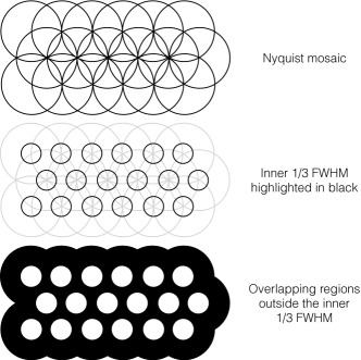
Figure 1.— Top: An illustration of a standard Nyquist mosaic, where the diameter of each circle indicates the FWHM of each pointing. Each pointing is centered at the FWHM of neighboring pointings. Middle: small black circles indicate the inner $\frac{1}{3}$ FWHM, where the off-axis polarization errors are minimal. Bottom: the black shaded region indicates the areas of the mosaic comprising emission that falls outside of the $\frac{1}{3}$ FWHM of any pointing.

Our target is the Kleinmann-Low Nebula in Orion (Orion-KL), which lies in the OMC-1 region at the center of the “integral-shaped filament,” a filamentary cloud with a length of $\gtrsim$ 7 pc that lies in the northern portion of the Orion A star-forming cloud (Johnstone & Bally, 1999). Our observations of Orion-KL comprise a mosaic centered on the iconic Source I (see, e.g., Plambeck et al., 2009, and references therein), and extending NNE and SSW to cover the filamentary structure, including the “Northern Ridge” (Johnstone & Bally, 1999; Hull et al., 2014) that lies $\sim$ 25$\arcsec$ to the NE of Source I. Later in this work, we compare our ALMA mosaics with a similar 1.3 mm linear-polarization mosaic of Orion-KL performed by Hull et al. (2014) using the Combined Array for Research in Millimeter-wave Astronomy (CARMA).

Single-dish polarization observations using the POL2 camera on the James Clerk Maxwell Telescope (JCMT) by Pattle et al. (2017) yielded a high-sensitivity image of the magnetic field in Orion A, which is roughly perpendicular to the filament’s long axis, as frequently seen in star-forming clouds whose magnetic field is thought to be dynamically important (e.g., Fissel et al., 2016; Planck Collaboration et al., 2016). These JCMT results, along with the results that we present here and in a companion paper (Cortes et al., 2020) are recent contributions to a large body of literature comprising single-dish and interferometric studies of millimeter, submillimeter, and far-infrared polarization toward the Orion-KL region and its environs. The first detection of polarization toward Orion-KL in this wavelength regime was made by a balloon-borne polarimeter (Cudlip et al., 1982); numerous later detections used polarimeters on the Kuiper Airborne Observatory (KAO), the Berkeley-Illinois-Maryland Association (BIMA) array, the JCMT, the Caltech Submillimeter Observatory (CSO), the Submillimeter Array (SMA), CARMA, the Stratospheric Observatory for Infrared Astronomy (SOFIA), and the IRAM 30 m telescope (Hildebrand et al., 1984; Novak et al., 1989; Rao et al., 1998; Schleuning, 1998; Plambeck et al., 2003; Girart et al., 2004; Houde et al., 2004; Matthews et al., 2009; Tang et al., 2010; Hull et al., 2014; Ritacco et al., 2017; Chuss et al., 2019). See Pattle et al. (2017) for a more exhaustive list of references.

Below we begin with a description of the observations, calibration, and imaging procedures for the 11$\times$11 observations of 3C 279 (§ II), after which we discuss the results from these tests (§ III). Similarly, we then present the mosaicked polarization observations toward Orion-KL (§ IV), and the results from those mosaic tests (§ V); the latter section includes a comparison between ALMA and CARMA observations toward Orion-KL (§ V.2). We end by offering our conclusions (§ VI).

All of the data we present here, and in a companion paper by Cortes et al. (2020), were collected as part of the ALMA Extension and Optimization of Capabilities (EOC) program. The EOC program is based at the Joint ALMA Observatory (JAO) in Santiago, Chile—with collaboration from scientists both at the ALMA Regional Centers (ARCs) as well as at external institutions—and is focused on using science-quality data to test, verify, and open new observing modes at ALMA.

Table 1Observational details (11$\times$11)

Band	Obs. date	Source	$N_{\textrm{ant}}$	UID
	(UTC)
3	2015 Mar 06	3C 279	31	A002_X9b98ec_X94d
				A002_X9b98ec_Xb98
				A002_X9b98ec_Xde3
5	2016 Nov 10	3C 279	9	A002_Xba6edb_X31db
				A002_Xba6edb_X3988
				A002_Xba6edb_X3d57
6	2015 May 08	3C 279	32	A002_Xa018c4_X743
				A002_Xa018c4_Xa3d
				A002_Xa018c4_Xdc7
7	2015 May 09	3C 279	35	A002_Xa018c4_X3b92
				A002_Xa018c4_X3de3
				A002_Xa018c4_X402a

II. 11$\times$11 observations of 3C 279

Our first set of observations comprise 11$\times$11 grids of offset pointings toward 3C 279 at Bands 3, 5, 6 and 7, the goal of which is to characterize the off-axis polarization errors across the field of view of single-pointing ALMA observations at several ALMA bands. The 11$\times$11 grid pointings are evenly spaced in (Azimuth, Elevation), and extend out to approximately the FWHM of the primary beam at each observing frequency. Figure 2 shows the pattern of the 121 pointings. Each set of observations of 3C 279 includes three separate executions spaced by $\sim$ 1 hr, which yields sufficient parallactic angle coverage to allow us to solve for the leakage terms ($D$-terms) and the cross-hand phase ($XY$-phase); we discuss the derivation of both of these quantities later in this section. We list the observation dates and data identification codes (or UIDs, each corresponding to an individual ALMA execution/observation) in Table 1. We chose to observe 3C 279 because, at the time of observation in 2015/2016, it was both extremely bright and had an extremely high linear polarization fraction. All observations were taken using the standard correlator setup for continuum polarization observations, which includes four 1.875 GHz-wide spectral windows with 64 channels each. See Table 2 for the on-axis results, and for the observational setup at each band.

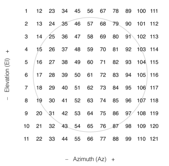
Figure 2.— 11$\times$11 pointing pattern. The dotted gray circle indicates the FWHM of the primary beam.

Table 2Observational setup and on-axis results (11$\times$11)

Band	$\nu$	$\theta$	Source	$I$	$Q$	$U$	$P_{\textrm{frac}}$	$\chi$
	(GHz)							(deg)
3	397.479	$3\farcs 31\times 2\farcs 49$	3C 279	1	0.0404	0.1074	0.115	34.7
5	183.261	$1\farcs 03\times 0\farcs 61$	3C 279	1	–0.00052	0.1095	0.110	045.1a
6	233.000	$1\farcs 15\times 0\farcs 88$	3C 279	1	0.0398	0.1142	0.121	35.4
7	343.479	$0\farcs 82\times 0\farcs 55$	3C 279	1	0.0373	0.1158	0.122	36.1

Note that, as no other calibrators besides 3C 279 were observed in the 11$\times$11 tests, we perform every step of the reduction process using 3C 279. We first split out the scans where 3C 279 was located at the pointing center (i.e., the central point of the 11$\times$11 grid) and concatenate them into a separate dataset; we use these on-axis data to derive the on-axis polarization calibration via the current ALMA polarization calibration scheme. For further details about standard, on-axis reduction of ALMA polarization data, see Nagai et al. (2016) as well as the 3C 286 Polarization CASA Guide.

We first perform an initial phase-versus-time gain calibration, which we apply on-the-fly when solving for the bandpass solution. After solving for the bandpass, we perform gain calibration (amplitude and phase), assuming an initial unpolarized source model for 3C 279. Since ALMA has crossed-linear feeds, the linear polarization properties of the source manifest themselves in the gain amplitude solutions when an initial, unpolarized model is used. To make a first estimate of the polarization of 3C 279, we use the task qufromgain from almapolhelpers.py. Next, we solve for the cross-hand delay using the scans where the $XX$/$YY$ polarization ratio is changing the fastest (this can be seen by viewing the gain-amplitude calibration table). We then solve for the $XY$-phase, which is the phase difference between the $X$ and the $Y$ polarizations of the reference antenna. This solution can have angle ambiguities, which we resolve by using the task xyamb; this task uses both the initial $XY$-phase solution as well as the previously derived initial model of the source polarization to solve for the final polarization model of 3C 279. With the correct model of 3C 279 in hand, we then re-derive the gains (amplitude and phase) using the model in order to remove the polarization response from the gain amplitudes. Finally, we derive the $D$-terms. After doing so, we apply all of the calibration tables (the bandpass; the modified gains after removing the source polarization; the cross-hand delay; the $XY$-phase; and the $D$-terms) to our on-axis dataset.

After applying the standard on-axis calibration to all of the on- and off-axis data, we perform one round of phase-only self-calibration (selfcal) to correct the residual phase errors as a function of time for both the on-axis data and each off-axis pointing. With the exception of the selfcal phase solutions, all calibration tables that we apply to the off-axis data are solved for using on-axis data only—this includes $D$-terms and $XY$-phase. We do this to mimic the standard calibration method of ALMA polarization data.

After completing the data reduction process, we produce $I$, $Q$, $U$, $V$ images using the task clean from CASA version 5.6.1 with standard imaging parameters, including a Briggs visibility weighting of robust = 2.0 (i.e., natural weighting). After making the images, we extract the $I$, $Q$, $U$, $V$ peak values using the CASA task imfit; these are the values that we analyze and report in Section III. Finally, we use these Stokes maps to produce maps of the linearly polarized intensity $P$, linear polarization fraction $P_{\textrm{frac}}$, and linear polarization angle $\chi$:

$$P=\sqrt{Q^{2}+U^{2}}$$ (1)

$$P_{\textrm{frac}}=\frac{P}{I}$$ (2)

$$\chi=\frac{1}{2}\,\textrm{arctan2}\,{\left(\frac{U}{Q}\right)}\,\,.$$ (3)

The dynamic range (peak flux value divided by the rms noise value) in the Stokes $I$ continuum maps ranges from $\sim$ 10,000–100,000, depending on the observing frequency (lowest dynamic range at Band 7, highest at Band 3). The dynamic range in the polarized intensity ($P$) maps is always a factor of $\sim$ 10 lower, since 3C 279 had a polarization fraction of $\sim$ 10% in all of our observations (see Table 2). Nevertheless, the dynamic range of our $P$ maps is always > 1000; in a region where the dynamic range of $P$ is 1000, the statistical error of the polarization angle ($\sigma_{\chi}=0.5\,\sigma_{P}/P$) is $\sim$ 0.03$\degree$, which is much smaller than the on-axis uncertainty of $\sim$ 0.4$\degree$ in the polarization angle calculated by Nagai et al. (2016) (Nagai et al. note that the exact value depends on the number of antennas used in each observation). Therefore, changes in the image properties of the $I,$ $Q,$ and $U$ Stokes parameters as a function of offset pointing are not caused by sensitivity limits, but rather by systematic polarization variations across the primary beam.

Since the time when these data were obtained 4–5 years ago, there have been no major changes in the receiver optics. The sub-reflectors in each antenna also remain un-tilted. A number of ALMA 12 m antennas were found to be astigmatic, which requires a corrective scheme to be applied to the surface of the dishes; however, as of the time of publication, this scheme has not yet been implemented. If the antenna astigmatism introduces wide-field polarization errors, then the errors reported in this work should improve once the correction scheme is applied. In the future, ALMA is planning new receivers, which will potentially change the optics (e.g., additional external mirrors) and will also use the tilting capabilities of the sub-reflector to improve the alignment with the receiver feeds. These changes will most likely improve the errors that we report here, but future tests will be needed to confirm this.

III. Results: 11$\times$11 observations of 3C 279

III.1. Error in $Q$, $U$, $P_{\textrm{frac}}$, and $\chi$

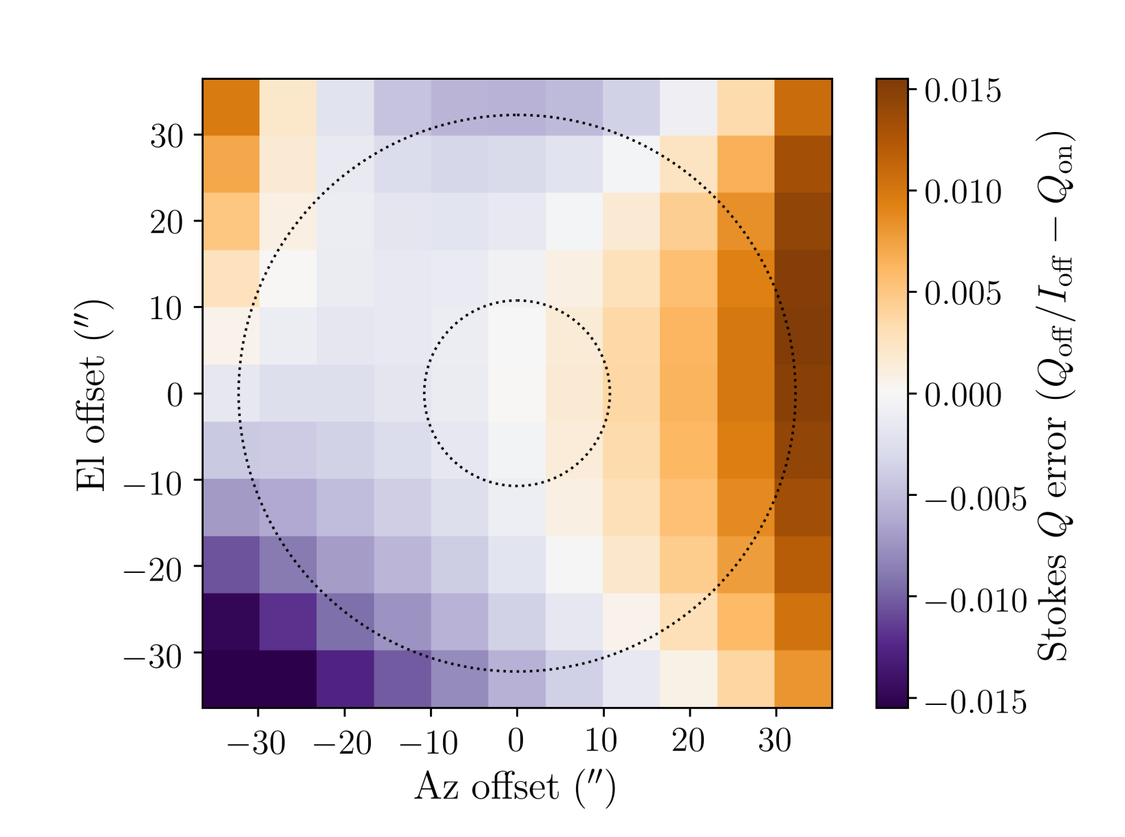
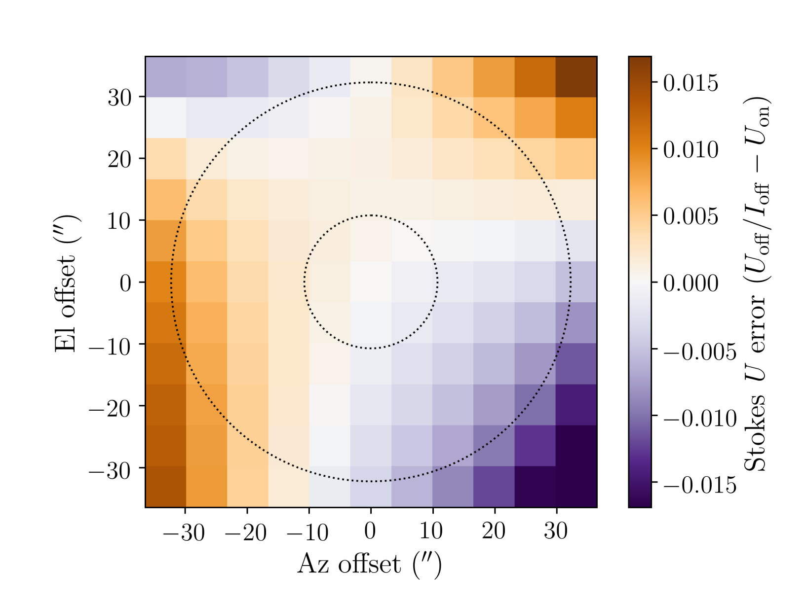
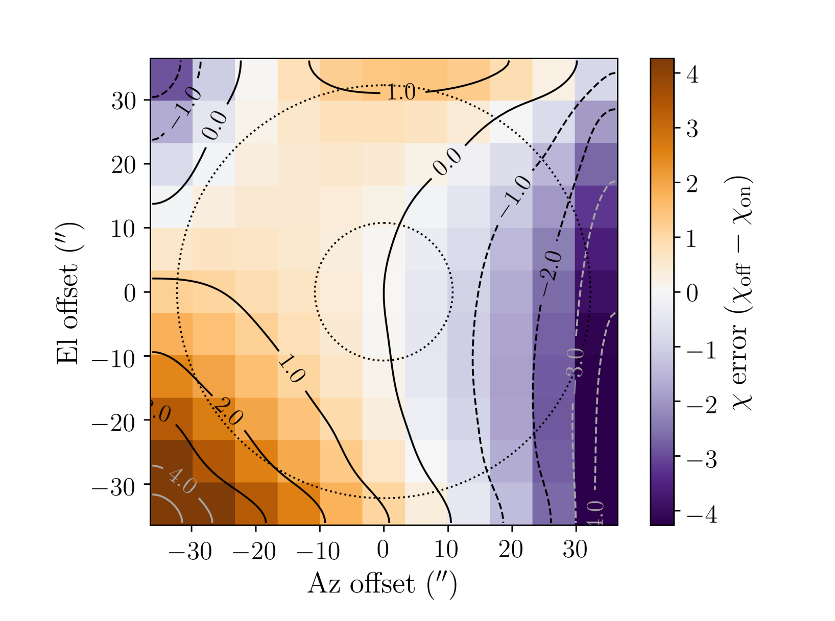
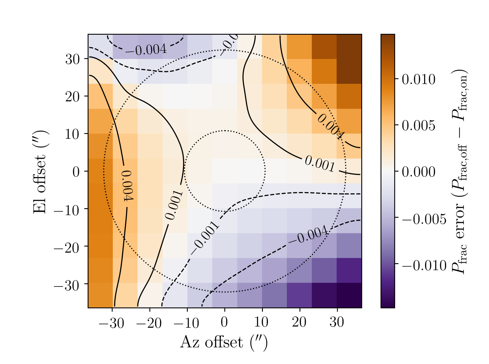
Figure 3.— Band 3 error maps in Stokes $Q,$ $U,$ position angle $\chi$, and polarization fraction $P_{\textrm{frac}}$. We apply on-axis calibration (including $D$-terms) to all off-axis positions. The outer dotted line is the FWHM of the primary beam; the inner dotted line is the $\frac{1}{3}$ FWHM level. The primary beam response was removed from the $Q$ and $U$ error maps by dividing by the Stokes $I$ value in each pixel. In all cases we subtract the central value from all of the off-axis pixels. The errors in $P_{\textrm{frac}}$ and $\chi$ shown in this figure (and similar figures for other bands) comprise the main results of the 11$\times$11 tests.

In Figure 3 (Band 3), and in Appendix A (Bands 5, 6, and 7), we show the errors across the primary beam in Stokes $Q$, Stokes $U$, $\chi$, and $P_{\textrm{frac}}$ that we derived from the observations toward the highly linearly polarized blazar 3C 279, which had $P_{\textrm{frac}}\approx 12\%$ at the time of observation. Assuming a circular, azimuthally symmetric primary beam in Stokes $I$, we can remove the primary beam response (i.e., the sensitivity fall-off with radius) in the Stokes $Q$ and $U$ images by dividing the off-axis Stokes $Q_{\textrm{off}}$ and $U_{\textrm{off}}$ values by the value of $I_{\textrm{off}}$ in the corresponding pixels:

$$Q_{\textrm{off,norm}} =Q_{\textrm{off}}/I_{\textrm{off}}$$ (4)

$$U_{\textrm{off,norm}} =U_{\textrm{off}}/I_{\textrm{off}}\,\,.$$ (5)

We then subtract the on-axis Stokes $Q_{\textrm{on}}$ or $U_{\textrm{on}}$ value from the normalized value in each pixel, leaving the residual errors $\delta Q$ and $\delta U$:

$$\delta Q =Q_{\textrm{off,norm}}-Q_{\textrm{on}}$$ (6)

$$\delta U =U_{\textrm{off,norm}}-U_{\textrm{on}}\,\,.$$ (7)

We define the off-axis $P_{\textrm{frac,off}}$ to be

$$P_{\textrm{frac,off}}=\frac{\sqrt{Q_{\textrm{off}}^{2}+U_{\textrm{off}}^{2}}}{I_{\textrm{off}}}\,\,.$$ (8)

As all of our Stokes $I$ maps are normalized to $I_{\textrm{on}}=1$, this simplifies the equations for $P_{\textrm{frac}}$:

$$P_{\textrm{frac,on}} =\sqrt{Q_{\textrm{on}}^{2}+U_{\textrm{on}}^{2}}$$ (9)

$$P_{\textrm{frac,off}} =\sqrt{Q_{\textrm{off,norm}}^{2}+U_{\textrm{off,norm}}^{2}}\,\,.$$ (10)

Finally, we calculate the error in the position angle $\delta\chi$ and in the polarization fraction $\delta P_{\textrm{frac}}$ as the differences in the on- versus off-axis pointings:

$$\delta\chi =\chi_{\textrm{off}}-\chi_{\textrm{on}}$$ (11)

$$\delta P_{\textrm{frac}} =P_{\textrm{frac,off}}-P_{\textrm{frac,on}}\,\,.$$ (12)

In the error maps of $\chi$ and $P_{\textrm{frac}}$, we subtract the central value from each pixel.

After analyzing the observations of the highly linearly polarized blazar 3C 279, we find that the systematic errors in the polarization fraction $\delta P_{\textrm{frac}}$ and in the position angle $\delta\chi$ are similar for all observing frequencies. Within the inner $\frac{1}{3}$ FWHM, the residual errors in $P_{\textrm{frac}}$ and $\chi$ are $\lesssim$ 0.001 ($\lesssim$ 0.1% of Stokes $I$) and $\lesssim$ 1$\degree$, respectively. Near the FWHM, the errors increase to $\sim$ 0.003–0.005 ($\sim$ 0.3–0.5% of Stokes $I$) and $\sim$ 1–5$\degree$, respectively, as shown in Figures 3, 10, 11, and 12.

III.2. $V$ beam shape (beam squint)

Each Stokes $V$ map exhibits a double-lobed “beam squint” pattern at the 1–2% level of the on-axis Stokes $I$ value: see Figure 4 (note that the Stokes $V$ values have not been primary-beam corrected). Squint arises when a receiver is not aligned with the telescope’s optical axis (Chu & Turrin, 1973; Adatia & Rudge, 1975; Rudge & Adatia, 1978). This is the case for all ALMA receivers, which are installed in a single dewar along several concentric circles, all of which are offset from the optical axis (Lamb et al., 2001). When dual-polarization receivers are offset, the response to left- and right-circular polarization (LCP and RCP, respectively) are slightly displaced from one another (this is true regardless of whether the receivers are crossed-linear like those at ALMA, or circular like, e.g., the 1.3 mm receivers at CARMA). Since Stokes $V$ $\equiv$ RCP – LCP (IEEE, 1997), this offset in the circular-polarization response of the two separate receivers results in a double-lobed Stokes $V$ pattern.

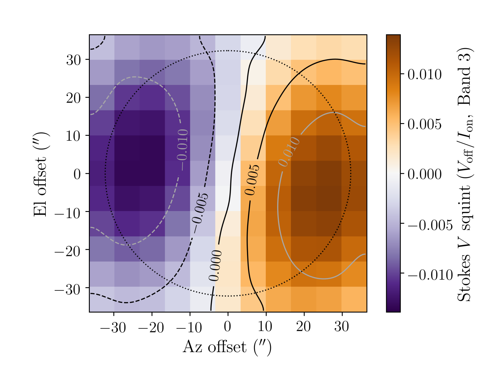
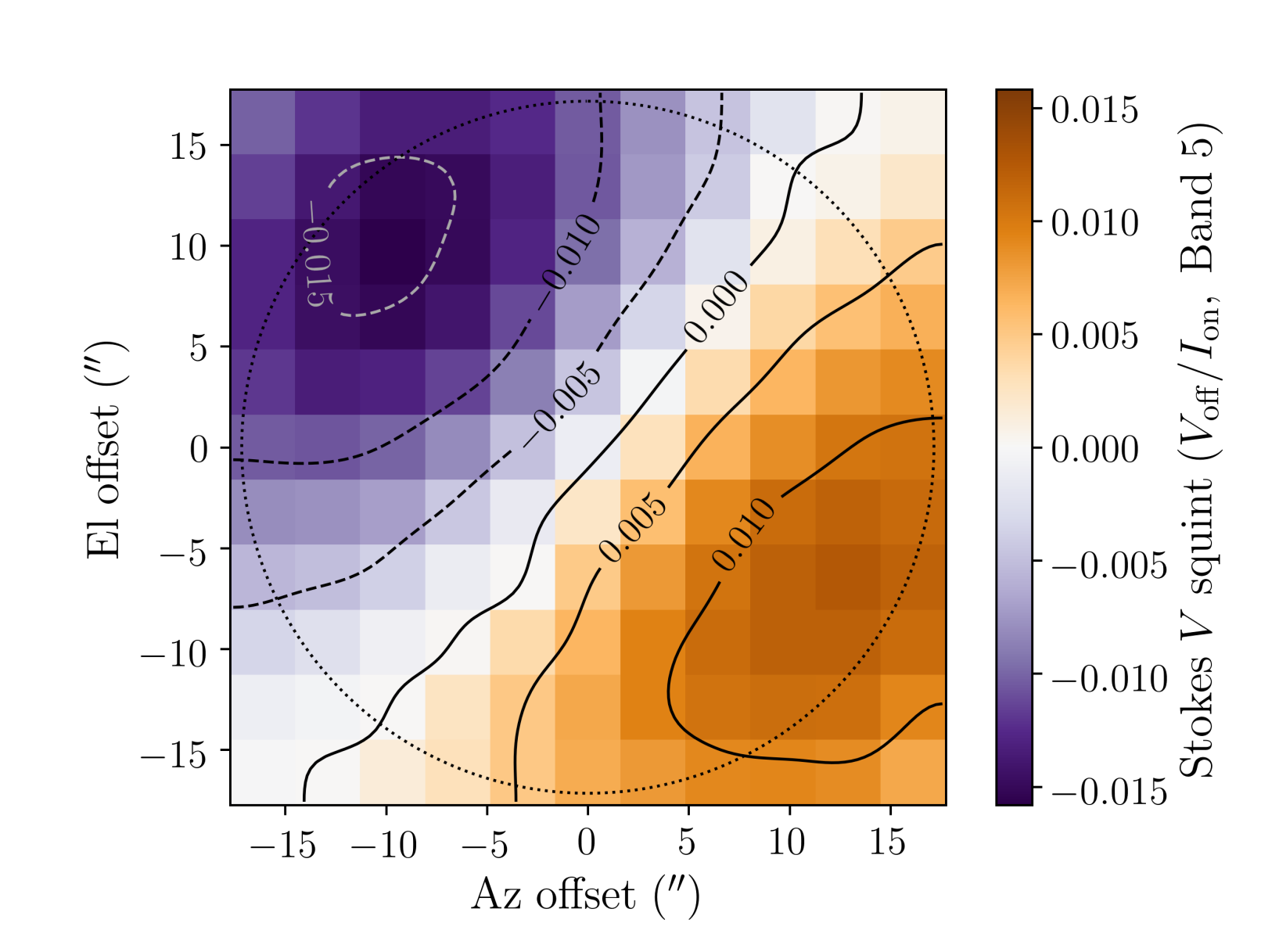
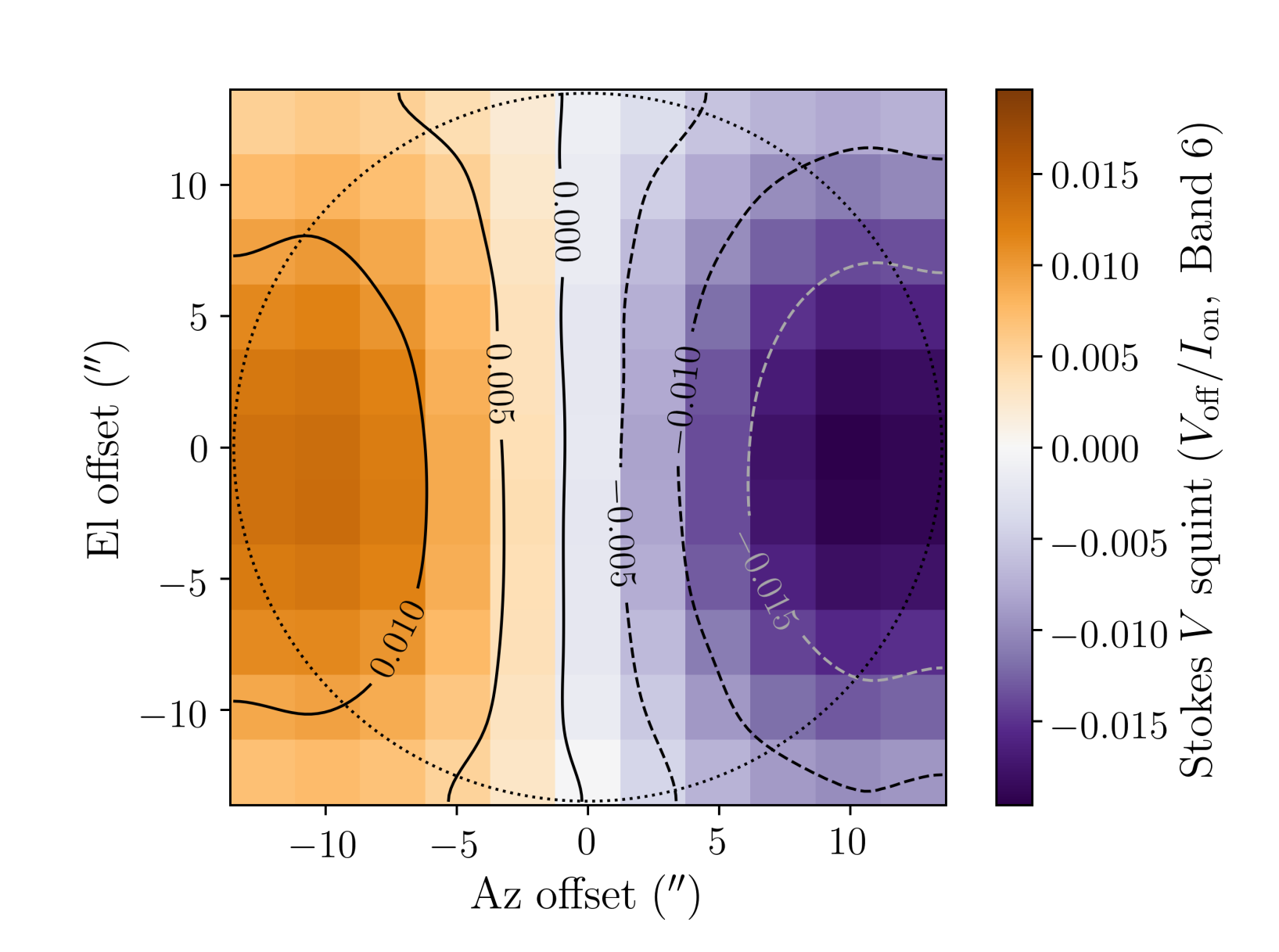
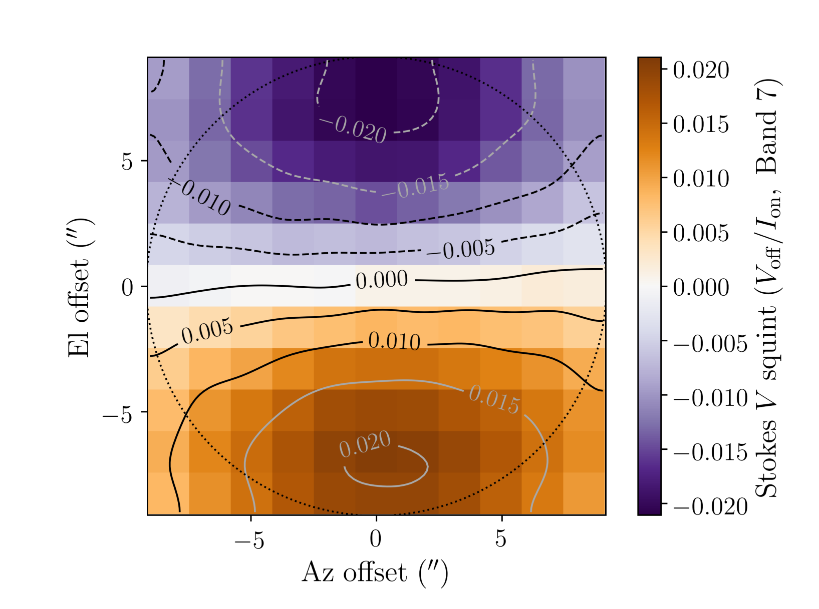
Figure 4.— Stokes $V$ squint profiles for Bands 3 (upper-left), 5 (upper-right), 6 (lower-left), and 7 (lower-right). Colorscale shows $V/I_{\textrm{on}}$, where the on-axis value $I_{\textrm{on}}$ has been normalized to 1. Note that the Stokes $V$ values have not been primary-beam corrected.

It is essential to correct for the known squint profile before attempting wide-field circular polarization observations (either mosaics or single pointings) with ALMA. This is particularly true because unlike the more extended “squash” error pattern in the linearly polarized $Q$ and $U$ maps (see Section III.3), the squint profile is compact, manifesting itself well within the FWHM at all bands. Direction-dependent errors such as squint can be removed from VLA observations using the awproject keyword in the CASA task tclean (Bhatnagar et al., 2008); however, this has not yet been implemented for ALMA observations. Efforts to implement full-polarization voltage-pattern corrections (i.e., primary beam models) at ALMA are underway (S. Bhatnagar et al., in preparation), and will allow us in the future to calibrate out the wide-field polarization errors that we analyze in this paper.

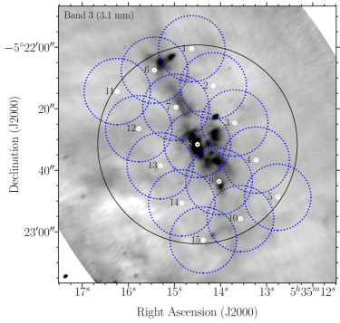
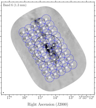
Figure 5.— Complete patterns for the Band 3 (left) and Band 6 (right) Orion-KL mosaics. The small white circles indicate the center of each field, the dotted blue circles correspond to the inner $\frac{1}{3}$ FWHM region of the 12 m antenna primary beam, and the solid black circle denotes the FWHM of the primary beam at the representative frequency of the observations. The ellipses in the lower-left corners are the synthesized beams (resolution elements), which measure 1$\farcs$43 $\times$ 0$\farcs$95 at Band 3 and 0$\farcs$65 $\times$ 0$\farcs$48 at Band 6.

III.3. $Q$ and $U$ errors (beam squash)

The maps of the off-axis errors in $Q$ and $U$ in some of the 11$\times$11 observations reveal hints of what is known as “beam squash,” which is a cloverleaf-like pattern in the Stokes $Q$ and $U$ error maps. Like beam squint, beam squash is caused by the antenna optics. Squash is the result of different beam widths of the orthogonal linear polarizations, which are in turn due to the varying projected geometries of the reflections over the parabolic reflector surface. Beam squash is discussed in Napier (1994, 1999), and can be seen in maps made using the Arecibo Observatory (Heiles et al., 2001) and the Green Bank Telescope (GBT; Robishaw & Heiles, 2018). Astroholography measurements show that the beam squash error patterns of the ALMA antennas have an angular extent of approximately twice that of the squint pattern (S. Bhatnagar et al., in preparation), and thus the extent of the 11$\times$11 observations is not sufficient to sample the entire pattern. However, particularly in the Band 3 data (Figure 3) and Band 7 data (Figure 12), we begin to see the inner edge of the cloverleaf pattern in the error maps of $Q$ and $U$, with four lobes alternating between positive and negative. We can also see the telltale 45$\degree$ rotation between the $Q$ and $U$ error patterns. The squash error patterns of the ALMA antennas will be investigated more thoroughly in future studies focusing on full-polarization holographic mapping of the full ALMA primary beam (S. Bhatnagar et al., in preparation).

IV. Orion-KL mosaic observations

We observed Orion-KL using the 12 m array at Bands 3 and 6. The data were taken in the standard sessions mode used for ALMA polarization observations (Remijan et al., 2019), and had the standard correlator setup for continuum polarization observations, which includes four 1.875 GHz-wide spectral windows with 64 channels each. The Band 3 and Band 6 sessions comprised three and two executions, respectively. We list the details in Table 3.

Table 3Observational details (Orion-KL)

Band	$\nu$	Obs. date	Source	Config.	$\theta$	$N_{\textrm{ant}}$	UID
	(GHz)	(UTC)
3	97.479	2018 Mar 17	Orion-KL	C-4	$1\farcs 43\times 0\farcs 95$	39	A002_Xca795f_X50f
		2018 Mar 18					A002_Xca795f_Xcbd
		2018 Mar 18					A002_Xca795f_Xd0
6	233.000	2019 Apr 12	Orion-KL	C-3 $\rightarrow$ C-4	$0\farcs 65\times 0\farcs 48$	43	A002_Xdab261_X13a0a
		2019 Apr 12					A002_Xdab261_X1448a

Table 4Pointings associated with the different Orion-KL mosaic patterns

Patterns	Band	Nyquist parameter	Pointing
Hyper-Nyquist	3	4.6	1 $\rightarrow$ 15, all pointings
Super-Nyquist	3	3.3	2, 4, 6, 8, 10, 12, 14
Nyquist	3	2.3	6, 8, 10
Single pointing	3	—	8
Hyper-Nyquist	6	4.6	1 $\rightarrow$ 45, all pointings
Super-Nyquist	6	3.3	2, 4, 6, 8, 10, 12, 14, 16, 18, 20, 22, 24, 26, 28, 30, 32, 34, 36, 38, 40, 42, 44
Nyquist	6	2.3	2, 4, 12, 14, 22, 24, 32, 34, 42, 44

We calibrate the data using the standard procedures for processing ALMA polarization observations (see, e.g., Cortes et al. 2016; Nagai et al. 2016; Hull et al. 2017, 2018). We use J0522–3627 as the polarization calibrator, J0423–0120 as the bandpass calibrator, and J0529–0519 as the gain calibrator. The same calibration sources were used in both the Band 3 and 6 observations. A bandpass scan was performed only in the first execution of the observing session. We derive the bandpass solutions and the flux scaling from both the bandpass calibrator (J0423–0120) and the polarization calibrator (J0522–3627), whereas we correct the amplitude and phase by deriving complex gains from the gain calibrator (J0529–0519). The polarization calibrator (J0522–3627) was observed every $\sim$ 35 minutes, and had a flux of 8.2 Jy and $P_{\textrm{frac}}\approx$ 3.4% during the Band 3 observations, and a flux of 3.8 Jy and $P_{\textrm{frac}}\approx$ 1.7% during the Band 6 observations.

The mosaicked observations of Orion-KL were set up to allow us to compare different mosaic patterns, which we label according to their different densities of pointings: Hyper-Nyquist (separation between the pointings of $\sim$ $1/4$ of the FWHM; i.e., over-sampled by a factor of $\sim$ 2 in each dimension relative to a standard Nyquist-sampled mosaic), Super-Nyquist (separation of $\sim$ $1/3$ of the FWHM; i.e., over-sampled by a factor of $\sim$ 1.5), Nyquist (separation of $\sim$ $1/2$ of the FWHM; i.e., standard sampling), and a single field (the reference pointing, centered on Source I itself).

The primary beam of each mosaic pointing is assumed (in CASA) to be a 2D Gaussian peaked at the center of the pointing. Figure 5 shows the full 3$\times$5 pointing rectangular mosaic pattern of our observations (i.e., the Hyper-Nyquist pattern) at Band 3, and the similar $5\times 9$ pattern at Band 6. In the case of Band 3, the field of view of the single pointing includes most of the filament, which allows us to compare the single pointing with the various ALMA mosaics. In contrast, the ALMA Band 6 field of view is too small to allow us to comparison the single pointing and the mosaics.

We image the data using the task tclean from CASA version 5.4.0, using standard imaging parameters and a Briggs visibility weighting of robust = 0.5, resulting in maps with synthesized beams (resolution elements) of 1$\farcs$43 $\times$ 0$\farcs$95 at Band 3 and 0$\farcs$65 $\times$ 0$\farcs$48 at Band 6. We independently image all four cases (i.e., Hyper-Nyquist, Super-Nyquist, Nyquist, and single field) in order to compare them with one another. We perform the imaging of all of these cases by specifying the fields that belong to each of the mosaic sampling patterns (see Table 4). For Band 3, all of the mosaicking patterns include the center field. In the Band 6 data, however, the Nyquist and Super-Nyquist mosaics do not include the center field. Consequently, we re-grid these latter mosaicked images to the Hyper-Nyquist frame using the CASA task imregrid in order to match the coordinates.

For each of the four patterns, we clean the Stokes $I$, $Q$, and $U$ maps separately. Note that we do not perform self-calibration on any of the images of Orion-KL. Furthermore, note that spectral lines were not flagged prior to making the continuum images (the default Band 6 spectral setup avoids major lines of interest). We primary-beam correct the final images using the CASA task impbcor to the 20% sensitivity level of the Stokes $I$ primary beam model. We then use these Stokes maps to produce maps of $P$, $P_{\textrm{frac}}$, and $\chi$. The mosaicked images of Orion-KL at both Bands 3 and 6 have median levels of $P_{\textrm{frac}}\approx 6-7\%$ across the maps. While the signal-to-noise ratio (SNR) of the $P$ images can be > 30 at the peaks of polarized emission, the median SNR values across the $P$ maps at Bands 3 and 6 are between 7–8.

V. Results: Orion-KL mosaic observations

In order to assess the performance of the ALMA’s linear-polarization mosaicking mode in a typical observational scenario, we performed standard (RA, DEC) observations of the Orion-KL star-forming region at Bands 3 and 6, and compare the images made using a single pointing versus the three different mosaic patterns (Hyper-Nyquist, Super-Nyquist, and Nyquist). Table 5 lists the peak fluxes and rms noise levels in the $I$, $Q$, $U$, and $P$ maps for both bands and all sampling patterns.

Table 5Image statistics from Orion-KL observations

Pattern	Band	$I_{\textrm{peak}}$	$I_{\textrm{rms}}$	$Q_{\textrm{peak}}$	$Q_{\textrm{rms}}$	$U_{\textrm{peak}}$	$U_{\textrm{rms}}$	$P_{\textrm{peak}}$	$P_{\textrm{rms}}$
		$\left(\frac{\textrm{mJy}}{\textrm{beam}}\right)$	$\left(\frac{\textrm{mJy}}{\textrm{beam}}\right)$	$\left(\frac{\textrm{mJy}}{\textrm{beam}}\right)$	$\left(\frac{\textrm{mJy}}{\textrm{beam}}\right)$	$\left(\frac{\textrm{mJy}}{\textrm{beam}}\right)$	$\left(\frac{\textrm{mJy}}{\textrm{beam}}\right)$	$\left(\frac{\textrm{mJy}}{\textrm{beam}}\right)$	$\left(\frac{\textrm{mJy}}{\textrm{beam}}\right)$
Hyper-Nyquist	3	112	0.90	–3.39	0.100	3.73	0.102	3.79	0.157
Super-Nyquist	3	112	0.93	–3.40	0.102	3.72	0.107	3.78	0.164
Nyquist	3	113	0.96	–3.47	0.118	3.75	0.120	3.81	0.180
Single field	3	115	1.31	–3.46	0.150	3.34	0.139	3.35	0.243
Hyper-Nyquist	6	415	2.08	11.30	0.522	12.300	0.495	13.500	0.485
Super-Nyquist	6	418	2.11	11.40	0.535	12.100	0.508	13.500	0.519
Nyquist	6	418	2.40	11.40	0.556	12.200	0.524	13.600	0.755

We first focus our analysis on comparing mosaicked images with the inner $\frac{1}{3}$ FWHM region of the single pointings, where the effects of residual off-axis errors are minimal. For both the Band 3 and Band 6 data, we analyze several individual pointings that are common to all three of the mosaics (see Table 4) and that show emission in $I$, $Q$, and $U$. We first produce difference maps (i.e., Hyper-Nyquist minus single pointing, Super-Nyquist minus single pointing, and Nyquist minus single pointing) for $I$, $Q$, and $U$ using the CASA task immath. We perform our comparison both with and without a cutoff, where the cutoff limits the difference images to the region(s) where the emission in the single pointing images is 5 $\times$ the rms noise level. We then use the CASA task imsubimage to extract the inner $\frac{1}{3}$ FWHM regions from the difference maps in order to quantify the impact of overlapping pointings in the mosaics, under the initial assumption that by stitching together pointings to make a mosaic, the emission in the mosaic should be “polluted” by the off-axis contributions from neighboring pointings (however, as we see later, we are not actually able to detect the effects of the off-axis pointings in the on-axis data).

We do not show the distributions of the differences in the Stokes $I$, $Q$, and $U$ maps here because all three difference histograms (for example, the three histograms of the differences in Stokes $Q$ between the chosen single pointing versus the Hyper-Nyquist, Super-Nyquist, and Nyquist mosaics) have similar structure, and have standard deviations that tend to be well below the rms noise level in the single-pointing images. This suggests that we can consider all of the mosaicked images to be the same when compared with the single pointing. Note also that the maps are dynamic range limited; in no case have we reached the thermal noise limit. These findings allow us to draw two main conclusions: first, the errors in the inner $\frac{1}{3}$ FWHM of the $Q$ and $U$ (and also $I$) maps are primarily caused by imaging artifacts stemming from the inability of our ALMA observations to recover emission at large spatial scales in Orion-KL, rather than by residual off-axis polarization errors; if the latter were dominant, we should expect to see a change in the width of the $Q$ and $U$ difference histograms with increased mosaic packing, since increased packing should reduce the contribution from off-axis errors. Second, while packing the pointings in the mosaics more closely should in theory improve the accuracy of the polarization images, we are not able to detect these incremental improvements among the Nyquist, Super-Nyquist, and Hyper-Nyquist mosaics. Thus, based on our dynamic-range-limited Orion-KL images (and for other sources with similarly complex, multi-scale structure), we cannot recommend using a mosaic packing that is tighter than the standard Nyquist pattern.

When analyzing the Orion-KL results, we choose not to analyze the fractional polarization errors, as the fractional polarization is equal to $\sqrt{Q^{2}+U^{2}}/I$; with respect to Stokes $I$, Stokes $Q$ and $U$ have different physical origins and thus different spatial structure (including different distributions of power as a function of spatial scale) when the source is resolved (for example, see the polarized intensity $P$ versus Stokes $I$ emission in high-resolution ALMA polarization maps in, e.g., Maury et al., 2018; Cortes et al., 2019; Hull et al., 2020; Le Gouellec et al., 2019). Finally, the Stokes $Q$ and $U$ maps have very different dynamic range limitations compared with the Stokes $I$ maps. Consequently, characterization of polarization fraction errors is better performed with point sources, as we have done in the 11$\times$11 observations of 3C 279 (see Section III.1).

We thus choose only to use the polarization position angle $\chi$ to characterize the effects of residual off-axis errors in the Orion-KL mosaics. Below we analyze $\chi$ only for the lower-resolution Band 3 data, because of the simplicity afforded by the larger field of view relative to Band 6, and because the large-scale structure in the Band 3 data is significantly less spatially filtered than in the higher resolution Band 6 data, resulting in lower-level imaging artifacts.

V.1. Comparison of $\chi$ in the mosaics versus the inner region ($r~{}<~{}\frac{1}{3}$ FWHM) and outer “donut” region ($\frac{1}{3}$ FWHM $<~{}r~{}<$ FWHM) of single pointings

We compute difference maps of the polarization position angle $\chi$ in the Hyper-Nyquist mosaic versus single-pointing images in the same manner as described above. The three single pointings we use are those in the Band 3 Nyquist mosaic; the setup of the test can be seen in Figure 6. We use a conservative (5 $\sigma_{P}$) cutoff in the $\chi$ maps in order to avoid considering any spurious points at the edge of the maps in our statistics.

The histograms of the $\chi$ differences within the inner $\frac{1}{3}$ FWHM of the single pointings can be seen in Figure 7. They all have standard deviations of < 1.3$\degree$, revealing that at the $\sim$ 1$\degree$ level, the regions of the mosaic corresponding to the inner $\frac{1}{3}$ FWHM region of a given pointing are not, in fact, “polluted” by the off-axis regions of the neighboring pointings, as we had initially assumed.

In Figure 7 we also show the histograms of the $\chi$ differences in the outer “donut” regions ($\frac{1}{3}$ FWHM $<~{}r~{}<$ FWHM). It is clear that in the two outer pointings (point 6 and point 10), the histograms of the differences in $\chi$ in the “donut” regions are significantly wider than in the inner $\frac{1}{3}$ FWHM regions, having standard deviations of 3.6$\degree$ (point 6) and 2.7$\degree$ (point 10). This suggests that we can detect the effects of residual off-axis errors in these single-pointing maps, consistent with what was seen in the 11$\times$11 maps.

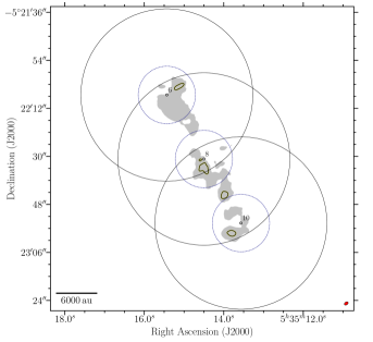
Figure 6.— Setup of the test to compare the polarization position angles in the three mosaics with those in the “donut”-shaped region outside of the $\frac{1}{3}$ FWHM in the three single pointings comprising the Band 3 Nyquist mosaic. The gray shaded area indicates the region where polarized emission is detected in the hyper-Nyquist mosaic map of Orion KL, and is masked below 5 $\sigma_{P}$, where the rms noise in the $P$ map $\sigma_{P}=0.15$ mJy beam^-1. Thick black contours indicate the regions where the $P$ map has SNR > 15. The concentric circles show the FWHM (large circles) and the $\frac{1}{3}$ FWHM (small circles) for the three different single pointings. The synthesized beam is shown as an ellipse in the lower-right corner.

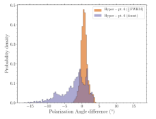
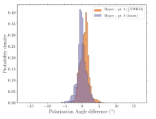
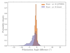
Figure 7.— Difference maps between the polarization position angle $\chi$ from three individual pointings in the Band 3 observations versus the same regions in the Hyper-Nyquist mosaic. The histograms show the differences in the inner $\frac{1}{3}$ FWHM as well as in the outer “donut” region ($\frac{1}{3}$ FWHM $<r<$ FWHM).

Mosaicking reduces these off-axis errors as a result of overlapping multiple pointings. A visually simple demonstration of this error-canceling effect can be seen by looking at Figure 6. In all three pointings, the median differences in $\chi$ in the high-SNR patches of polarized emission (see the thick contours in Figure 6, which inducate regions where $P$ has an SNR > 15, corresponding to a statistical uncertainty of $\sim$ 2$\degree$)—when observed by the Hyper-Nyquist mosaic versus when observed on-axis in the single pointings—are always < 1$\degree$. However, for example, when the patch of emission near the center of point 6 is observed near the FWHM of point 8 (i.e., when the emission is observed off-axis), the median difference with respect to the Hyper-Nyquist mosaic is $\sim$ 3$\degree$, as expected from the Band 3 11$\times$11 tests (see Figure 3). This same effect is also seen when the other patches of high-SNR emission near the centers of points 8 and 10 are observed off-axis: the median position angle difference with respect to the Hyper-Nyquist mosaic when the emission is observed off-axis in the single pointings is always larger than the difference when the same emission is observed on-axis. These simple tests demonstrate again that mosaicking the image reduces the off-axis polarization angle errors.

Note that, in an effort to connect these Orion-KL error results with the errors we derived from the 11$\times$11 blazar observations (see Section III.1), we perform a statistical analysis of the 11$\times$11 data. This analysis, which is an attempt to estimate the errors in a mosaic from the 11$\times$11 data, can be found in Appendix B.

V.2. Comparison with CARMA

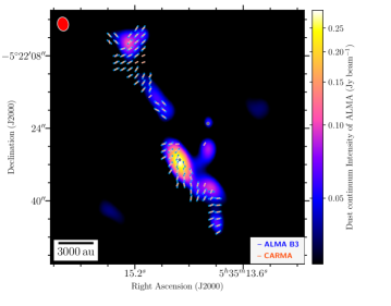
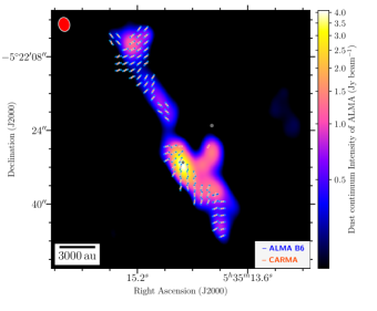
Figure 8.— Comparison of ALMA and CARMA observations of the inferred magnetic field (rotated by 90$\degree$ with respect to the observed polarization) toward Orion-KL using the Nyquist-sampled ALMA data (blue line segments) and CARMA data (orange line segments). Both maps show the same 1.3 mm CARMA data; the left- and right-hand maps show the Band 3 (3 mm) and Band 6 (1.3 mm) ALMA data, respectively. We produce both ALMA maps using the same $uv$-coverage as the CARMA observations, and then smooth them to the CARMA beam size of 3$\farcs$07$\,\times\,$2$\farcs$45 (shown as ellipses in the upper-left corners of both plots). The color scales show the Stokes $I$ thermal dust emission from ALMA, which we plot beginning at 3 $\sigma_{I}$, where $\sigma_{I}$ is the rms noise in the smoothed ALMA maps. $\sigma_{I}=8.9$ mJy beam^-1 at Band 3 and 55 mJy beam^-1 at Band 6. The CARMA polarization map is the one provided in the online version of Hull et al. (2014, see their Figure 19); the map was already masked, and thus we perform no additional cuts. We plot the ALMA polarization detections only in locations with a corresponding CARMA detection. The diamond and circle indicate the positions of Source I and the Becklin-Neugebauer Object (BN; Becklin & Neugebauer, 1967), respectively, plotted at the positions reported in Rodríguez et al. (2017). The distance to the Orion Nebula Cluster is $388\pm 5$ pc (Kounkel et al., 2017).

Another mosaicked polarization observation of Orion-KL was performed by Hull et al. (2014) using the CARMA interferometer’s full-polarization system (Hull & Plambeck, 2015). Here we compare those archival data from an independent instrument with our ALMA results in order to characterize the performance of ALMA linear-polarization mosaics. The 1.3 mm CARMA data were taken in 2013, have a resolution of 3$\farcs$07$\,\times\,$2$\farcs$45, and comprise a seven-pointing mosaic with a field of view similar to that of our ALMA observations. In order to perform the most accurate possible comparison between the CARMA and ALMA datasets, we match the $uv$-range (using the uvrange keyword in the CASA task clean) and the synthesized-beam size (using the CASA task imsmooth) of the Band 3 and Band 6 ALMA data to those of CARMA. We also re-grid the ALMA images to match the coordinates of the CARMA maps. We use the standard Nyquist mosaic pattern from our ALMA data for the comparison with the CARMA observations, which are also Nyquist sampled.

See Figure 8 for an overlay of the inferred magnetic field from the CARMA data with both the Band 3 and Band 6 ALMA data. We can see that the magnetic field orientation in both the Band 3 and the Band 6 ALMA maps matches the CARMA observations remarkably well, especially in the Northern Ridge. This consistency of inferred magnetic field orientation as a function of frequency is expected in optically thin material (which, we should note, might not be the case toward the very central region near Source I), under the standard assumption that dust-grain alignment via radiative alignment torques (RATs; Lazarian, 2007) is the cause of the dust polarization.

In Figure 9 we show both a map and a histogram of the differences in the polarization position angle $\chi$ in the ALMA versus the CARMA data. The distribution of differences peaks around 0$\degree$, with a width (defined as the minimum window necessary to encompass 68% of the data) of $\pm$ 12$\degree$. The differences in $\chi$ can be as large as $\pm$ 40$\degree$ in some locations, and the distribution is somewhat skewed to negative differences, but there is no obvious systematic trend in angle differences in the CARMA versus ALMA maps. The ALMA polarization position angles have a systematic error of < 1$\degree$ on-axis (Nagai et al., 2016). The CARMA polarization position angle measurements have a systematic on-axis error of $\pm$ 3$\degree$, which is the result of systematic errors in the $XY$-phase correction (including variations in the absolute position angle of the wire grids used to derive the $XY$-phase passbands; Hull & Plambeck 2015).

VI. Conclusions

We characterize the wide-field errors in interferometric observations performed using the ALMA array of 12 m antennas. We first measure the errors across the field of view of a single-pointing image by observing the highly linearly polarized blazar 3C 279 in 11$\times$11 grids out to the FWHM of primary beam in the (Azimuth, Elevation) frame. Next, in order to characterize ALMA’s polarization mosaic performance during a standard-mode observation in the (RA, DEC) frame, we performed mosaicked linear-polarization observations at Bands 3 and 6 of the Orion-KL star-forming region using several different mosaic patterns.

These are the main conclusions we draw from the 11$\times$11 observations of the highly linearly polarized blazar 3C 279:

[1.] After on-axis calibration of all off-axis pointings, we find that:

[(a)] The systematic errors in polarization fraction ($P_{\textrm{frac,err}}=P_{\textrm{frac,on}}-P_{\textrm{frac,off}}$) for all observed bands (3, 5, 6, 7) are $\lesssim$ 0.001 ($\lesssim$ 0.1% of Stokes $I$) near the beam center, and increase to $\sim$ 0.003–0.005 ($\sim$ 0.3–0.5% of Stokes $I$) near the FWHM of the primary beam.

[(b)] The systematic errors in the polarization position angle ($\chi_{\textrm{err}}=\chi_{\textrm{on}}-\chi_{\textrm{off}}$) are $\lesssim$ 1$\degree$ near the beam center, and $\sim$ 1–5$\degree$ near the FWHM.

[2.] In all bands, we see the expected double-lobed “beam squint” patterns in the Stokes $V$ maps at the 1–2% level of Stokes $I$.

[3.] The off-axis errors in the $\chi$ and $P_{\textrm{frac}}$ maps arise from differences in the shapes of the $Q$ and $U$ beams. Also known as “beam squash,” this effect causes cloverleaf patterns of positive and negative lobes in the $Q$ and $U$ error maps. The quadrupolar squash error patterns are approximately twice the linear extent of the double-lobed beam squint patterns, and thus our 11$\times$11 observations only sample the inner part of the squash error patterns.

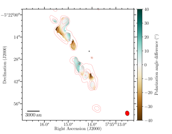
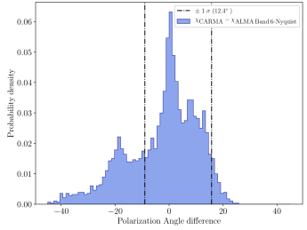
Figure 9.— Left: Map of the differences in the polarization position angle $\chi$ between the Nyquist-sampled ALMA Band 6 image of Orion-KL and the 1.3 mm CARMA map from Hull et al. (2014). The red contours show the polarized intensity $P$ in the ALMA data, which we plot at 3, 5, 9 $\times$ $\sigma_{P}$, where $\sigma_{P}=3.9$ mJy beam^-1 in the smoothed ALMA map, as derived from the Python astropy.stats.mad_std method. Note that as in Figure 8, we normalize $\sigma_{P}$ by the primary-beam-correction map. We plot the diamond, circle, and ellipse (synthesized beam) as in Figure 8. Right: histogram of the differences in $\chi$ in the CARMA versus ALMA maps. We only include pixels whose polarized intensity is $\geq$ 5 $\times$ $\sigma_{P}$ of the ALMA data. The map from Hull et al. (2014) was already masked based on the SNR of its polarized intensity. The two black, dot-dashed lines encompass 68% of the distribution; the width of the distribution, defined as half the distance between the two lines, is $\sim$ 12$\degree$.

Next, we analyze linear-polarization mosaics of the Orion-KL star-forming region observed using several patterns: a single-pointing observation, a standard Nyquist-sampled mosaic, and two more densely packed (“Super-Nyquist” and “Hyper-Nyquist”) mosaics. While we conclude that mosaicking improves the accuracy of the polarization images relative to the single pointing images, we are not able to detect incremental improvements in the accuracy among the three mosaics. Thus, based on our Orion-KL images (and for other sources with similarly complex, multi-scale structure), we cannot recommend using a mosaic packing that is tighter than the standard Nyquist pattern. Finally, we compare the ALMA results with archival CARMA data. Our conclusions from these efforts are as follows:

[4.] We compare the Band 3 and Band 6 mosaicked images of Orion-KL with the inner $\frac{1}{3}$ FWHM region of several single pointings. We find that the errors in the inner $\frac{1}{3}$ FWHM of the $Q$ and $U$ (and also $I$) maps are primarily caused by imaging artifacts stemming from the inability of our ALMA observations to recover emission at large spatial scales in Orion-KL, rather than by residual off-axis polarization errors. Furthermore, the different spatial structure of the $I$ versus $Q$ and $U$ emission makes it difficult to perform a meaningful analysis of the differences in maps of $P_{\textrm{frac}}$. Characterization of errors in $P_{\textrm{frac}}$ is thus better performed with point sources, as we have done in the 11$\times$11 observations of 3C 279.

[5.] The polarization position angle $\chi$ is a better quantity for characterizing off-axis errors, as it is independent of $I$. The difference maps of $\chi$ in the (Band 3 only) Hyper-Nyquist mosaic versus the inner $\frac{1}{3}$ FWHM regions of three Band 3 single pointings show that the differences are $\sim$ 1$\degree$, indicating that, at the $\sim$ 1$\degree$ level, the inner regions of a given pointing are not “polluted” by the errors in the off-axis regions of neighboring pointings.

[6.] Next we compare the (Band 3 only) Hyper-Nyquist mosaic with the outer ($\frac{1}{3}$ FWHM < $r$ < FWHM) “donut” region of the same three Band 3 single pointings. We find that, in two of the three pointings, the distributions of the differences between $\chi$ in the outer “donut” regions of the single pointings versus the mosaic are significantly wider than the differences in the inner $\frac{1}{3}$ FWHM of the single pointings versus the mosaic. This suggests that we can detect the effects of off-axis errors in the single-pointing maps, consistent with what was seen in the 11$\times$11 tests.

[7.] We perform a simple test using the Band 3 Orion-KL data where we analyze several patches of high-SNR polarized emission. In all three pointings, the median differences in $\chi$ in the high-SNR patches of polarized emission—when observed by the Hyper-Nyquist mosaic versus when observed on-axis in the single pointings—are always < 1$\degree$. However, when the same patches of emission are viewed off-axis in adjacent single pointings, the median position angle differences with respect to the Hyper-Nyquist mosaic are always larger (with typical median values of 2–4$\degree$) than when the same emission is observed on-axis. These larger differences are consistent with the Band 3 11$\times$11 tests. These tests demonstrate again that mosaicking reduces off-axis errors.

[8.] Finally, we perform a comparison of both the 3 mm and 1.3 mm ALMA mosaics with a 1.3 mm CARMA mosaic from Hull et al. (2014). After matching the $uv$-coverage of the ALMA and CARMA data and then smoothing the ALMA data to the coarser CARMA resolution, we find good consistency in the polarization position angles in both bands, especially in the Northern Ridge region of Orion-KL. The distribution of differences in $\chi$ in the CARMA versus the ALMA maps has a width of $\pm$ 12$\degree$.

Our results show that, due to the large angular extent of the beam-squash pattern of the ALMA 12 m antennas, the errors introduced by this wide-field effect are modest. We show that mosaicking reduces the magnitudes of these errors because multiple pointings are overlapped, and because the mosaic-imaging algorithm puts a higher weight on emission that is on-axis versus emission that is far from the pointing center. However, ultimately we would like to be able to calibrate out these effects, thus yielding accurate wide-field polarization images even in single-pointing observations. Efforts to implement full-polarization voltage-pattern corrections (i.e., primary beam models) at ALMA are underway, and will allow us to achieve this goal in the future.

A. A. Off-axis Stokes $I,Q,U,V$ data using the highly linearly polarized blazar 3C 279

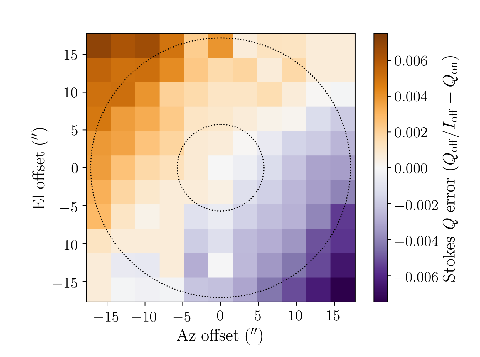
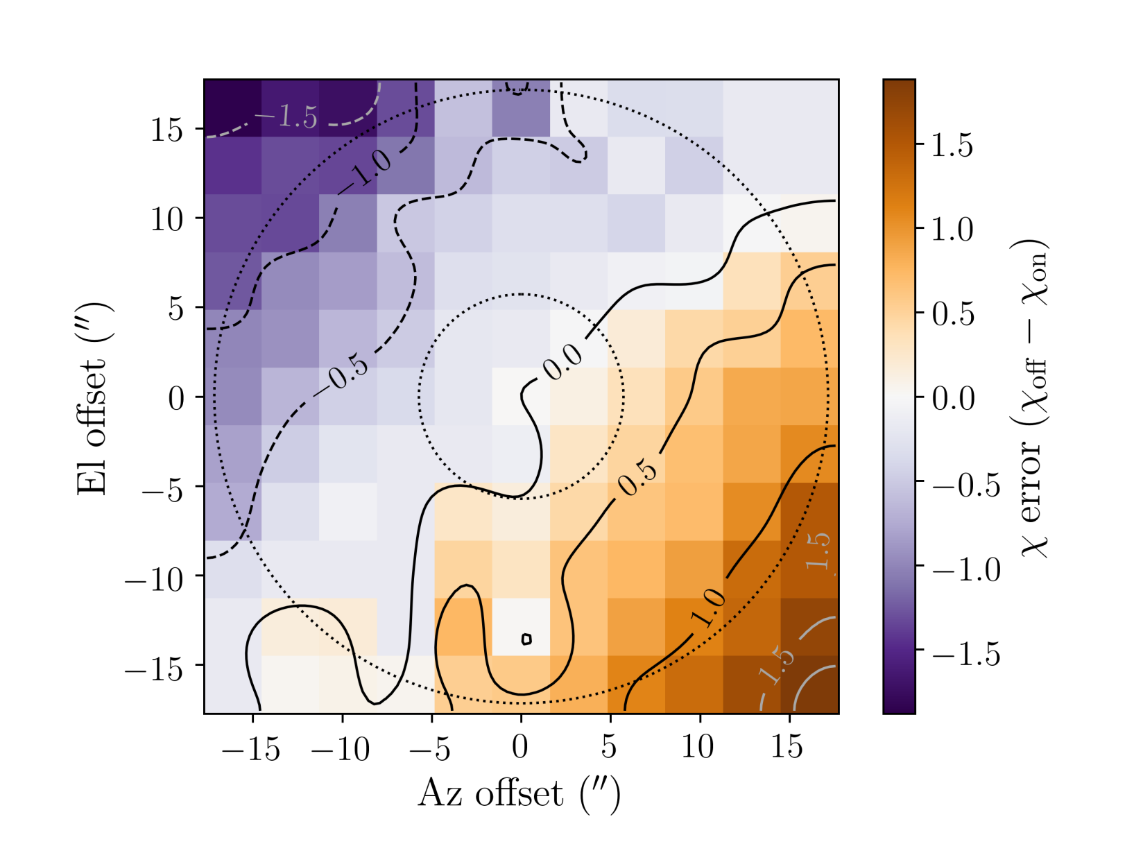
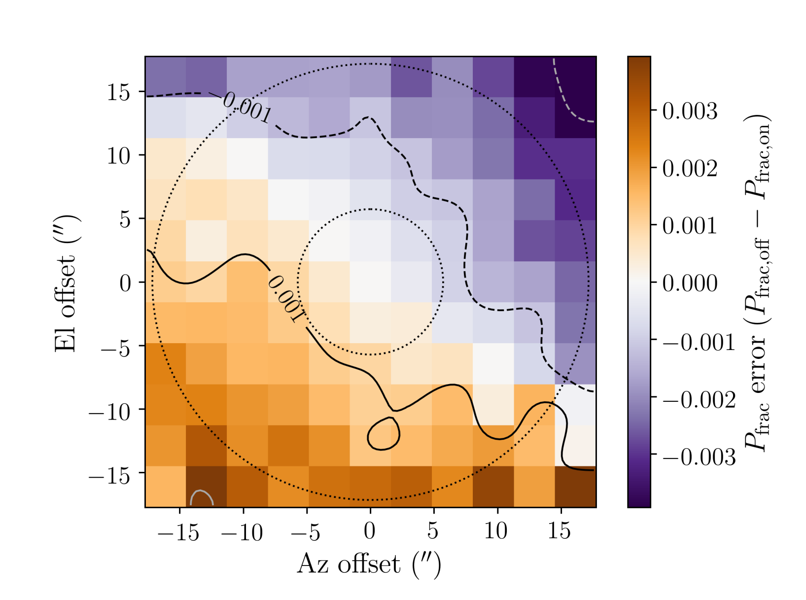
Figure 10.— Same as Figure 3, for Band 5.

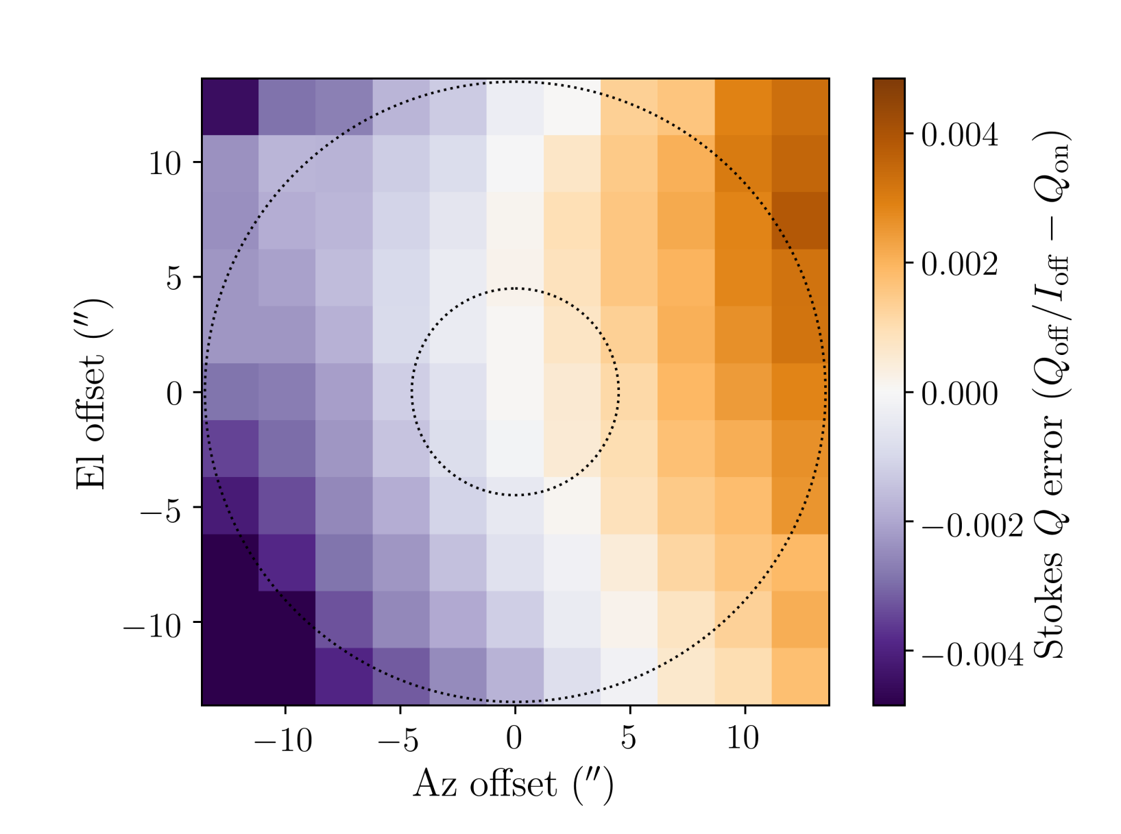
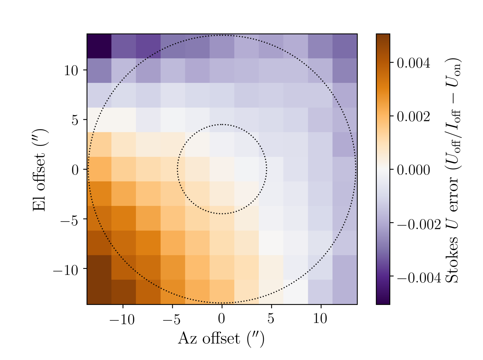
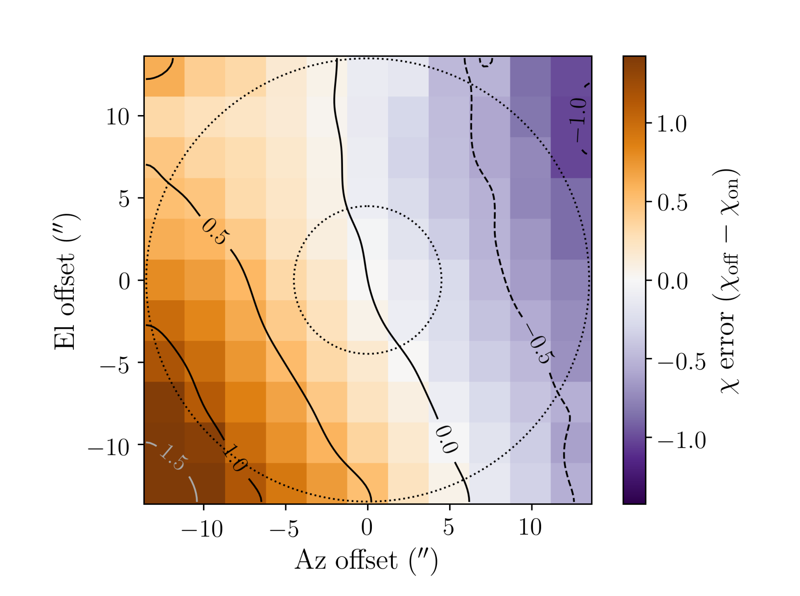
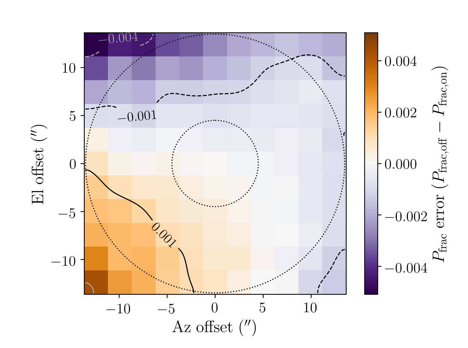
Figure 11.— Same as Figure 3, for Band 6.

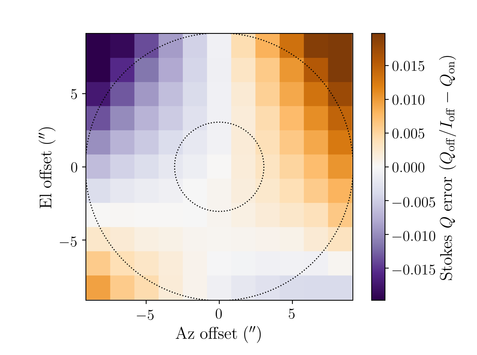
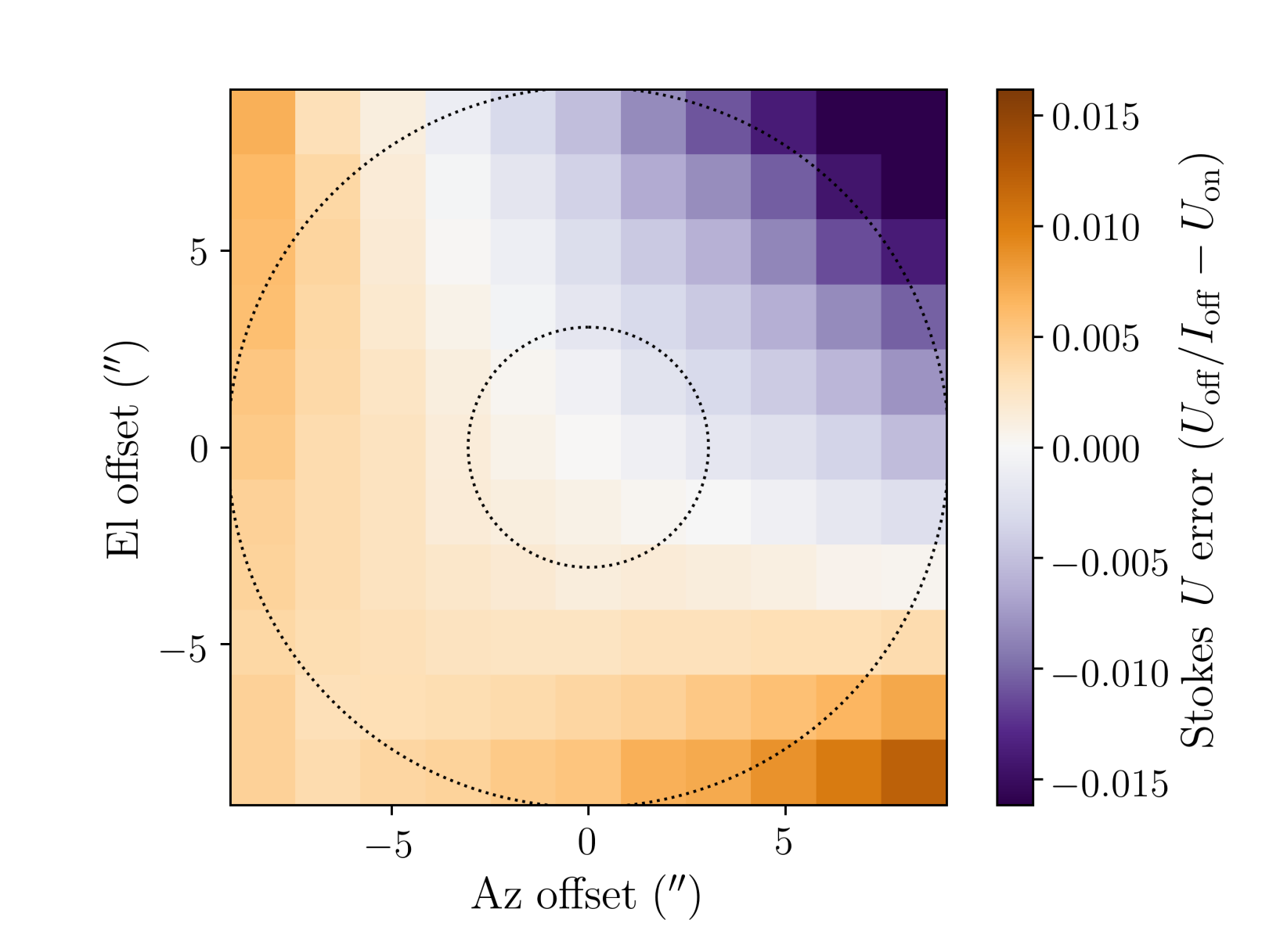
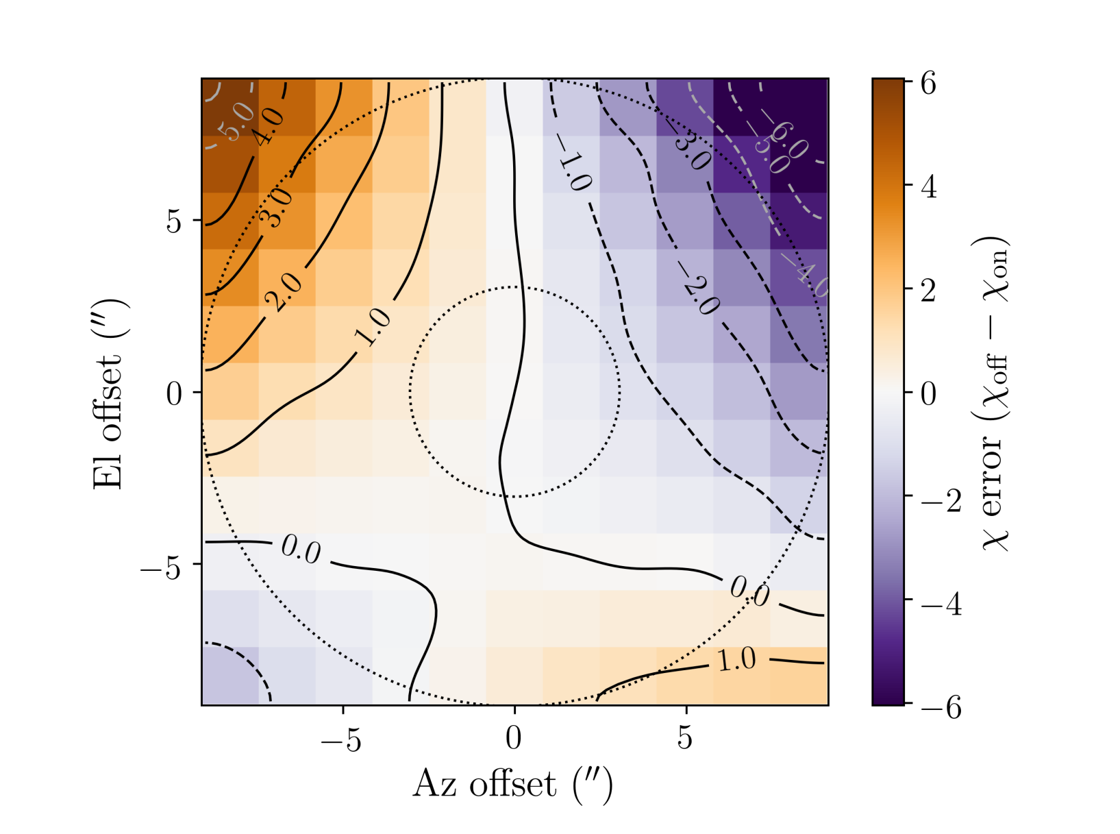
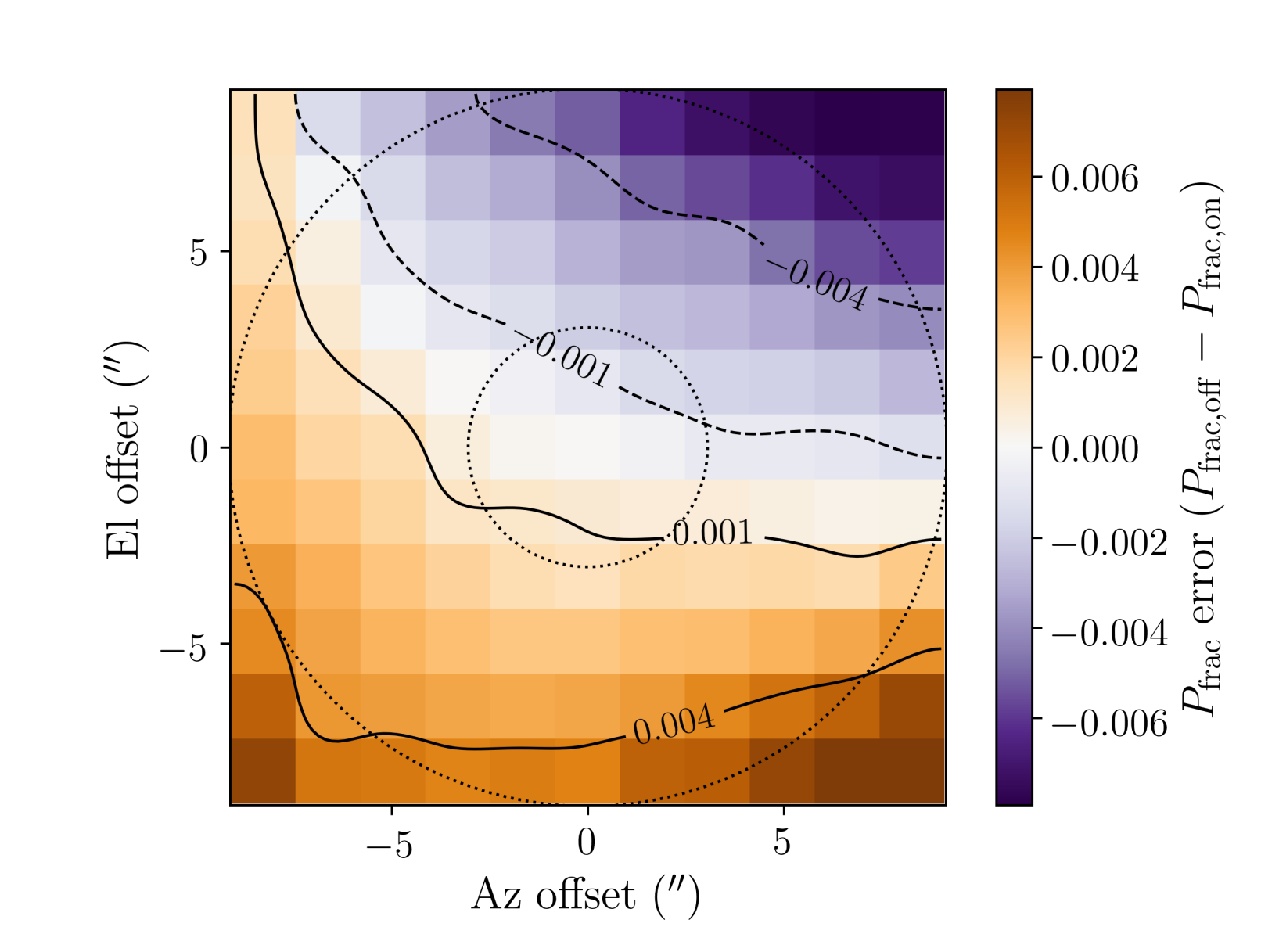
Figure 12.— Same as Figure 3, for Band 7.

B. B. Error estimates in a polarization mosaic using the 11$\times$11 observations

We perform a simple statistical analysis based on the the $11\times 11$ observations of the highly linearly polarized blazar 3C 279 (see Sections II and III) in order to use those data to estimate the errors in a polarization mosaic. These estimates are an effort to connect the 11$\times$11 results with the error results from the Orion-KL mosaic data that we report in Section V.

In single-pointing observations, the image can be divided into the inner region (which we define as $r\,<\,\frac{1}{3}$ FWHM) and the outer “donut” region ($r>\frac{1}{3}$ FWHM). The initial ALMA polarization capabilities only allowed observations of objects whose emission falls in the inner region, as polarization errors are known to increase further off-axis, as shown in this paper. However, in a mosaicked observation, neighboring pointings—each of which has varying polarization errors across its respective field of view—are stitched together, and thus the errors combine differently in different parts of the mosaic. While much of a standard Nyquist-mosaicked image will fall within the $\frac{1}{3}$ FWHM of a given pointing, there will still be a significant fraction of the image that will fall inside of the FWHM but outside of the $\frac{1}{3}$ FWHM region of any given pointing: see the filled black region in Figure 1. In many cases, the wide-field polarization errors in multiple pointings will cancel out, thus reducing the overall error in the mosaicked map; however, the cancellation depends on a number of different factors, including the error patterns in the Stokes $Q$ and $U$ maps, the timing and duration of the observations, the chosen mosaic packing pattern, and the orientation of the source on the sky.

In Section III we characterize the average polarized response of the primary beam of the 12 m array at Bands 3, 5, 6, and 7 by observing a blazar in an 11$\times$11 grid in the Az/El frame. We derive error maps in $Q$ and $U$ as well as in $\chi$ and $P_{\textrm{frac}}$. Here we use those results to estimate the average error in the regions of the mosaic that are composed of overlapping outer regions of neighboring pointings. In order to be conservative, in the analysis below we consider all of the data lying in the region $\frac{1}{3}$ FWHM < $r$ < FWHM. However, in practice, the data near the FWHM of a given pointing will be substantially down-weighted relative to the data from neighboring pointings, which will be closer to on-axis, since the center of each pointing in a Nyquist mosaic is located at the FWHM of its neighboring pointings.

Figure 13.— The black squares indicate the pointings whose data were considered in the error estimates discussed in this Appendix. As an illustration, they are overlaid on the $P_{\textrm{frac}}$ error map from the 11$\times$11 Band 3 test, whose original data are shown in Figure 3.

In order to estimate the error in the regions of a mosaic where multiple pointings overlap, we first use standard error propagation of the values in the maps of $\delta Q$ and $\delta U$. These values, $\sigma_{Q}$ and $\sigma_{U}$, are calculated simply as the standard deviation of the values of $\delta Q$ and $\delta U$ in the ring that lies outside of the $\frac{1}{3}$ FWHM, but inside the FWHM of a given pointing (see Figure 13 for a diagram of the chosen pointings). These $\sigma$ values correspond to estimators, in a statistical sense, of the “typical” errors in the off-axis $Q$ and $U$ values. We then average $\sigma_{Q}$ and $\sigma_{U}$ to estimate the systematic error $\sigma_{P}$ in the polarized intensity $P$; this is justified since, almost always, $\sigma_{Q}\approx\sigma_{U}$ (see Table 5). Thus, the error in the polarization fraction $\sigma_{\textrm{Pfrac}}$ can be approximated, using error propagation and the fact that $\sigma_{Q}\approx\sigma_{U}\equiv\sigma_{P}$, as:

$$\sigma_{\textrm{Pfrac}}=P_{\textrm{frac}}\sqrt{\left(\frac{\sigma_{P}}{P}\right)^{2}+\left(\frac{\sigma_{I}}{I}\right)^{2}}\,\,.$$ (1)

Given that $I$ is large relative to $P$ and assuming a circular, azimuthally symmetric primary beam (and thus no position-dependent systematic error $\sigma_{I}$), we set the second term to zero. This simplifies the equation to:

$$\sigma_{\textrm{Pfrac}}=P_{\textrm{frac}}\frac{\sigma_{P}}{P}\,\,,$$ (2)

which is identically equal to the error in the polarized intensity $\sigma_{P}$, since $P_{\textrm{frac}}=P/I$ and we define $I$ to be 1.

The error in the polarization angle $\chi$ is:

$$\sigma_{\chi}=\frac{0.5}{P^{2}}\sqrt{\left(Q\,\sigma_{U}\right)^{2}+\left(U\,\sigma_{Q}\right)^{2}}\,\,.$$ (3)

By again assuming that $\sigma_{Q}\approx\sigma_{U}\equiv\sigma_{P}$, we can simplify the equation to:

$$\sigma_{\chi}=0.5\frac{\sigma_{P}}{P}\,\,.$$ (4)

Using these equations, we can estimate the typical error in $P_{\textrm{frac}}$ and $\chi$ in the areas indicated in Figure 13. See Table 6 for these values, which have superscript ^a.

In addition to error propagation, another way to estimate the typical error in $P_{\textrm{frac}}$ and $\chi$ is to calculate directly the standard deviation of the values in the $\delta P_{\textrm{frac}}$ and $\delta\chi$ error maps. See Table 6: these values, denoted by superscript ^b, are the same as the values derived from error propagation to within factors of < 40% ($\sigma_{\textrm{Pfrac}}$) and < 30% ($\sigma_{\chi}$). As mentioned above, the resulting errors are conservatively large, as they are derived from the entire region between the $\frac{1}{3}$ FWHM and the FWHM.

Table 6Errors in 11$\times$11 maps toward highly linearly polarized 3C 279

Band	$\sigma_{Q}$	$\sigma_{U}$	$\sigma_{P}$	$\sigma_{\textrm{Pfrac}}^{a}$	$\sigma_{\chi}^{a}$	$\sigma_{\textrm{Pfrac}}^{b}$	$\sigma_{\chi}^{b}$
					(deg)		(deg)
3	0.0040	0.0032	0.0036	0.0036	0.90	0.0025	1.1
5	0.0020	0.0013	0.0016	0.0016	0.43	0.0013	0.52
6	0.0016	0.0012	0.0014	0.0014	0.33	0.00085	0.43
7	0.0041	0.0032	0.0037	0.0037	0.86	0.0024	1.1

References

- Adatia & Rudge (1975) Adatia, N. A., & Rudge, A. W. 1975, Electronics Letters, 11, 513
- Astropy Collaboration et al. (2018) Astropy Collaboration, Price-Whelan, A. M., Sipőcz, B. M., et al. 2018, AJ, 156, 123
- Becklin & Neugebauer (1967) Becklin, E. E., & Neugebauer, G. 1967, ApJ, 147, 799
- Bhatnagar et al. (2008) Bhatnagar, S., Cornwell, T. J., Golap, K., & Uson, J. M. 2008, A&A, 487, 419
- Chu & Turrin (1973) Chu, T.-S., & Turrin, R. 1973, IEEE Transactions on Antennas and Propagation, 21, 339
- Chuss et al. (2019) Chuss, D. T., Andersson, B. G., Bally, J., et al. 2019, ApJ, 872, 187
- Cortes et al. (2016) Cortes, P. C., Girart, J. M., Hull, C. L. H., et al. 2016, ApJ, 825, L15
- Cortes et al. (2019) Cortes, P. C., Hull, C. L. H., Girart, J. M., et al. 2019, ApJ, 884, 48
- Cortes et al. (2020) Cortes, P. C., Le Gouellec, V. J. M., Hull, C. L. H., et al. 2020, ApJ, in preparation
- Cudlip et al. (1982) Cudlip, W., Furniss, I., King, K. J., & Jennings, R. E. 1982, MNRAS, 200, 1169
- Fissel et al. (2016) Fissel, L. M., Ade, P. A. R., Angilè, F. E., et al. 2016, ApJ, 824, 134
- Girart et al. (2004) Girart, J. M., Greaves, J. S., Crutcher, R. M., & Lai, S.-P. 2004, Ap&SS, 292, 119
- Harp et al. (2011) Harp, G. R., Ackermann, R. F., Nadler, Z. J., et al. 2011, IEEE Transactions on Antennas and Propagation, 59, 2004
- Heiles et al. (2001) Heiles, C., Perillat, P., Nolan, M., et al. 2001, PASP, 113, 1247
- Hildebrand et al. (1984) Hildebrand, R. H., Dragovan, M., & Novak, G. 1984, ApJ, 284, L51
- Houde et al. (2004) Houde, M., Dowell, C. D., Hildebrand, R. H., et al. 2004, ApJ, 604, 717
- Hull et al. (2020) Hull, C. L. H., Gouellec, V. J. M. L., Girart, J. M., Tobin, J. J., & Bourke, T. L. 2020, The Astrophysical Journal, 892, 152
- Hull & Plambeck (2015) Hull, C. L. H., & Plambeck, R. L. 2015, Journal of Astronomical Instrumentation, 4, 1550005
- Hull et al. (2014) Hull, C. L. H., Plambeck, R. L., Kwon, W., et al. 2014, ApJS, 213, 13
- Hull et al. (2017) Hull, C. L. H., Girart, J. M., Tychoniec, Ł., et al. 2017, ApJ, 847, 92
- Hull et al. (2018) Hull, C. L. H., Yang, H., Li, Z.-Y., et al. 2018, ApJ, 860, 82
- IEEE (1997) IEEE. 1997, IEEE Std 211-1997, doi:10.1109/IEEESTD.1998.87897
- Jagannathan et al. (2017) Jagannathan, P., Bhatnagar, S., Rau, U., & Taylor, A. R. 2017, AJ, 154, 56
- Johnstone & Bally (1999) Johnstone, D., & Bally, J. 1999, ApJ, 510, L49
- Kounkel et al. (2017) Kounkel, M., Hartmann, L., Loinard, L., et al. 2017, ApJ, 834, 142
- Lamb et al. (2001) Lamb, J. W., Baryshev, A., Carter, M. C. C., et al. 2001, ALMA Memo Series, 362
- Lazarian (2007) Lazarian, A. 2007, J. Quant. Spec. Radiat. Transf., 106, 225
- Le Gouellec et al. (2019) Le Gouellec, V. J. M., Hull, C. L. H., Maury, A. J., et al. 2019, ApJ, 885, 106
- Matthews et al. (2009) Matthews, B. C., McPhee, C. A., Fissel, L. M., & Curran, R. L. 2009, ApJS, 182, 143
- Maury et al. (2018) Maury, A. J., Girart, J. M., Zhang, Q., et al. 2018, MNRAS, 477, 2760
- McMullin et al. (2007) McMullin, J. P., Waters, B., Schiebel, D., Young, W., & Golap, K. 2007, in Astronomical Society of the Pacific Conference Series, Vol. 376, Astronomical Data Analysis Software and Systems XVI, ed. R. A. Shaw, F. Hill, & D. J. Bell, 127
- Nagai et al. (2016) Nagai, H., Nakanishi, K., Paladino, R., et al. 2016, ApJ, 824, 132
- Napier (1994) Napier, P. J. 1994, ALMA Memo Series, 115
- Napier (1999) Napier, P. J. 1999, in Astronomical Society of the Pacific Conference Series, Vol. 180, Synthesis Imaging in Radio Astronomy II, ed. G. B. Taylor, C. L. Carilli, & R. A. Perley, 37
- Novak et al. (1989) Novak, G., Gonatas, D. P., Hildebrand, R. H., Platt, S. R., & Dragovan, M. 1989, ApJ, 345, 802
- Pattle et al. (2017) Pattle, K., Ward-Thompson, D., Berry, D., et al. 2017, ApJ, 846, 122
- Perley (2016) Perley, R. A. 2016, EVLA Memos, 195
- Plambeck et al. (2003) Plambeck, R. L., Wright, M. C. H., & Rao, R. 2003, ApJ, 594, 911
- Plambeck et al. (2009) Plambeck, R. L., Wright, M. C. H., Friedel, D. N., et al. 2009, ApJ, 704, L25
- Planck Collaboration et al. (2016) Planck Collaboration, Ade, P. A. R., Aghanim, N., et al. 2016, A&A, 586, A138
- Rao et al. (1998) Rao, R., Crutcher, R. M., Plambeck, R. L., & Wright, M. C. H. 1998, ApJ, 502, L75
- Remijan et al. (2019) Remijan, A., Biggs, A., Cortés, P., et al. 2019, ALMA Technical Handbook (ALMA Doc. 6.3, ver. 1.0)
- Ritacco et al. (2017) Ritacco, A., Ponthieu, N., Catalano, A., et al. 2017, A&A, 599, A34
- Robishaw & Heiles (2018) Robishaw, T., & Heiles, C. 2018, ArXiv e-prints, arXiv:1806.07391
- Robitaille & Bressert (2012) Robitaille, T., & Bressert, E. 2012, APLpy: Astronomical Plotting Library in Python, Astrophysics Source Code Library, ascl:1208.017
- Rodríguez et al. (2017) Rodríguez, L. F., Dzib, S. A., Loinard, L., et al. 2017, ApJ, 834, 140
- Rudge & Adatia (1978) Rudge, A. W., & Adatia, N. A. 1978, IEEE Proceedings, 66, 1592
- Schleuning (1998) Schleuning, D. A. 1998, ApJ, 493, 811
- Tang et al. (2010) Tang, Y.-W., Ho, P. T. P., Koch, P. M., & Rao, R. 2010, ApJ, 717, 1262
- Thompson et al. (2017) Thompson, A. R., Moran, J. M., & Swenson, George W., J. 2017, Interferometry and Synthesis in Radio Astronomy, 3rd Edition (Springer), doi:10.1007/978-3-319-44431-4
- Thum et al. (2018) Thum, C., Agudo, I., Molina, S. N., et al. 2018, MNRAS, 473, 2506