Hybrid Position/Force Control for Hydraulic Actuators

Abstract

In this paper a novel hybrid position/force control with autonomous switching between both control modes is introduced for hydraulic actuators. A hybrid position/force control structure with feed-forwarding, full-state feedback, including integral control error, pre-compensator of the dead-zone, and low-pass filtering of the control value is designed. Controller gains are obtained via local linearization and pole placement accomplished separately for the position and force control. A hysteresis-based autonomous switching is integrated into the closed control loop, while multiple Lyapunov function based approach is applied for stability analysis of the entire hybrid control system. Experimental evaluation is shown on the developed test setup with the standard industrial hydraulic cylinders, and that for different motion and load profiles.

I Introduction

Different actuators are in use in the mechatronic applications. While electric motors, linear drives, or pneumatic actuators are well suitable for a fast system response, hydraulic actuators are still the first choice if compact form factor combined with high power density and reliability are demanded, see [1, 2] for backgrounds. At the same time, hydraulic systems are also well known for their nonlinearities and associated challenges arising during operation in the closed-loop force or motion control.

Several applications using hydraulic actuators are repetitive and tedious for human operators, for example excavators, but remain yet to be controlled manually. While an, at least, semi-automatic control emerges in these fields, the widespread PID-controllers keep yet standard also in those applications. While improvements like for instance optimal design of PID-control with non-linear extensions were reported [3], other research promotes different control strategies like for example adaptive control or variable structure control, showing often a superior performance to the classic PID-controllers, see e.g. [4, 5, 6]. When a hydraulically actuated equipment or machine interacts with the environment, like given example of an excavator, a permanent use of position control can become even destructive due to inherently stiff control properties. In that case a force-based control approach is necessary. Several force control strategies for hydraulic systems were reported [7, 8, 9], while the force control issues are equally well-known in robotics and mechatronics, see e.g. [10]. However, for a fully automated operation of such equipment, a combination of force and position control should be taken into consideration, where the individual controllers can be switched, correspondingly reconfigured upon the motion constraints and interaction with the environment. Such hybrid control approaches remain topical, even though addressed generally in the former works, especially in the field of robotics, see e.g. [11, 12].

In this paper, a hybrid position and force control approach is pursued based on the feed-forwarding and full-state feedback, including the integral control error. An appropriate hysteresis-based switching strategy is integrated into the closed feedback loop, while changing between the parameter settings of both control modes. Remarkable is that the derived control structure self does not change and, therefore, represents an uniform architecture for the position and force control simultaneously.

The synthesized hybrid control relies on a detailed model of the system plant under consideration. In [13], a reduced hydraulic model related to the setup was derived which was expanded upon in [14], and the initial hybrid position-force control results reported in [15]. In the recent work, we present the fully elaborated hybrid position/force control with extended design, analysis, and evaluation. The rest of the paper is structured as following. In Section II the model from [14] is summarized while in Section III the proposed control architecture, control gains tuning, linearized system behavior, and local stability analysis based on [16] are described. An exhaustive experimental control evaluation is reported in Section IV with the paper’s summary given in Section V.

II System modeling

The modeled hydraulic system is a single rod, double acting cylinder connected to a servo valve which in return is connected to an HPU (Hydraulic Power Unit). The full model from [14] describes the second order valve dynamics, dead-zone-saturation combination, orifice and continuity equations, cylinder dynamics and Stribeck friction. The respective parameters and characteristics were identified and the simulation results validated by comparing with experimental data from different tests. A model reduction was performed under a mild assumption of equal cylinder cross sections, thus introducing a total load dependent pressure and flow. The control valve dynamics were neglected due to an observed unity gain in the frequency range of interest. Linearisation were performed of the form $g(x)\approx kx+d$, with $k$ being the slope and $d$ the offset of a linear function, whose nonlinear counterpart is $g(\cdot)$. The linearized, piecewise affine, state-space model of the plant is then given by

$$\dot{\textbf{x}} =\textbf{A}\textbf{x}+\textbf{b}u+\textbf{f},$$ (1)

$$y =\textbf{c}\textbf{x},$$

where $\textbf{x}=(x,\dot{x},P_{L},F_{L})^{T}$ is the state vector with $x$ being the cylinder position, $\dot{x}$ the cylinder velocity, $P_{L}$ the load dependent pressure and $F_{L}$ the external load force. The system matrix, input coupling, affine term, and output coupling vectors are given by

A $$=\begin{bmatrix}0&1&0&0\\[3.0pt] 0&-\begin{aligned} \frac{k_{w}}{m}\end{aligned}&\begin{aligned} \frac{\bar{A}}{m}\end{aligned}&-\begin{aligned} \frac{1}{m}\end{aligned}\\[3.0pt] \begin{aligned} 0\end{aligned}&\begin{aligned} -\frac{4E\bar{A}}{V_{t}}\end{aligned}&\begin{aligned} \frac{4E\hat{C}_{qp}}{V_{t}}\end{aligned}&\begin{aligned} 0\end{aligned}\\[3.0pt] 0&0&0&0\\ \end{bmatrix},$$ (2)

$$\begin{split}\textbf{b}=\begin{bmatrix}0\\[0.0pt] 0\\[0.0pt] \frac{4E\hat{C}_{q}k_{g}}{V_{t}}\\[0.0pt] 0\end{bmatrix},\end{split}\quad\begin{split}\textbf{f}=\begin{bmatrix}0\\[3.0pt] -\frac{d_{w}}{m}\\[0.0pt] \frac{4E\hat{C}_{q}d_{g}}{V_{t}}\\[0.0pt] 0\end{bmatrix},\end{split}\quad\begin{split}\textbf{c}^{T}=\begin{bmatrix}1\\[0.0pt] 0\\[0.0pt] 0\\[0.0pt] 0\end{bmatrix},\end{split}$$ (3)

correspondingly. Here $k_{w}$ and $d_{w}$ are coefficients of the linearized Stribeck function, $m$ is the lumped moving mass of the cylinder, $\bar{A}$ is the average cylinder cross section, $E$ is the hydraulic fluids bulk modulus, $V_{t}$ is the combined hydraulic fluids volume in the lines from the valve to the cylinder, $\hat{C}_{q}$ and $\hat{C}_{qp}$ are the coefficients of the linearized orifice equation and $k_{g}$ and $d_{g}$ are the coefficients of the linearized dead-zone and saturation combination. For more model details we refer to [14]. It is worth emphasizing that the modeled load force, as a state, provides zero eigen-dynamics since being an exogenous external quantity. Note that the above state-space model is configured here to have the piston position as the output value. This will be reconfigured when switching between the position and force control.

III Control Design

This section is dedicated to control design, while describing the overall hybrid closed-loop system. The determination of control parameters and local stability are also addressed. For details on the residual control components, such as feed-forward dead-zone compensation, signal filtering, and switching strategy we refer to [15] due to the space limitations.

III-A Hybrid control structure

The proposed control architecture includes the feed-forward, integral-error- and full-state-feedback. A more classical architecture would refer to a cascaded structure, where the inner-loop represents a force control and the outer-loop the position control. Such control approaches have certain inherent shortcoming. An ideal force control tends to zero control stiffness, while an ideal position control stiffness tends towards infinity. Therefore a cascaded combination would always constitute a tradeoff and offer a suboptimal performance when targeting the position and force control tasks simultaneously.

For enhancing the control performance of both operation modes, a hybrid switched position/force control is developed, see Fig. 1. Note that an additional vector of external disturbances $\Psi(t)$ is drawn, for the sake of completeness, although not explicitly modeled and analyzed, that due to a limited process knowledge. For the rest of the paper, $h$ represents the discrete switching variable and, therefore, the corresponding operation mode, with $h=-1$ for position and $h=1$ for force control. Note that the hybrid position/force control structure remains the same upon switching and allows for control parameters to be determined separately, so as to meet the performance requirements in both cases.

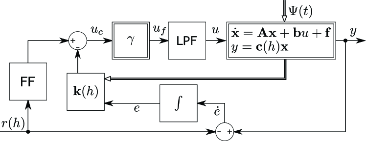
Figure 1: Block-diagram of the hybrid position/force control

For the closed-loop control system the state vector of (1) is extended by an additional integral control error state with $\dot{e}=y-r(h)$ dynamics, thus resulting in $\textbf{x}_{e}=(\textbf{x}^{T},e)^{T}$. Here $r(h)$ is the control reference value, while the output $y$ depends on the control mode and is switched through the output coupling vector $\mathbf{c}(h)$. Note that in order to accommodate the integral error state, the system matrix (2) and vectors (3) of the state-space model are directly extendable to $\mathbf{A}_{e}\in\mathbb{R}^{5\times 5}$ and $\mathbf{b}_{e},\mathbf{c}_{e}^{T},\mathbf{f}_{e}\in\mathbb{R}^{5\times 1}$. The resulting control law is then

$$u_{c}=\text{FF}\,r(h)-\textbf{k}(h)\mathbf{x}_{e},$$ (4)

where $\mathbf{k}(h)=(K_{1},K_{2},K_{3},K_{4},K_{i})$ is the vector of the control gains, which are determined separately for position and force control. FF represents the feed-forward control part, which is the single gain value for the given structure, and that FF $=K_{1}$ for position and FF $=K_{4}$ for force control. The overall control structure, cf. Fig. 1, includes also the pre-filtering dead-zone compensator $\gamma$ and the low-pass filtering (LPF) of the control signal, both addressed in [15].

III-B Determining of control gains

The control gain parameters are determined via standard pole placement accomplished for the linearized models, that separately for the position and force control modes. The pole placement is made for the test case scenarios, the same which are lately evaluated in the experiments. The controlled rod displacement is driven with a constant speed until it reaches a hard stop (by environment), that triggers an autonomous switching to the force control at which the rod is holding a constant force. Since the steady-state velocity and force are defined by reference, the residual state values required for the model linearization are extrapolated from the simulation of the full-order (nonlinear) model, cf. [14].

The state-space model (1) does not allow for directly using the pole placement, that due to inclusion of the affine terms. In order to deal with affine vector $\mathbf{f}_{e}$, that when deriving the state-space form applicable for a pole placement, the state vector is further extended to $\bar{\mathbf{x}}=[\mathbf{x}_{e}^{T},1]^{T}$, thus resulting in

$$\dot{\bar{\textbf{x}}}=\begin{bmatrix}\dot{\mathbf{x}}_{e}\\ 0\end{bmatrix}=\bar{\mathbf{A}}\bar{\mathbf{x}}+\bar{\mathbf{b}}\,r=\begin{bmatrix}\mathbf{A}_{e}&\mathbf{f}_{e}\\ \mathbf{0}&0\end{bmatrix}\bar{\mathbf{x}}+\begin{bmatrix}\mathbf{b}_{e}\\ 0\end{bmatrix}r,$$ (5)

while the output coupling vector is extended to $\bar{\mathbf{c}}=[\mathbf{c}_{e},0]$. This allows establishing the set of two state-space forms, where the switching discrete state $h=\left[-1,1\right]$ refers to the position and force control respectively. The overall hybrid control system, in the linearized form, is then given by

$$\dot{\bar{\textbf{x}}} =\bar{\textbf{A}}(h)\bar{\textbf{x}}+\bar{\textbf{b}}(h)r(h),$$ (6)

$$y =\bar{\textbf{c}}(h)\bar{\textbf{x}}.$$

Since the feedback control design relies on the linearized modeling at steady-state operational conditions, following assumptions, correspondingly simplifications, can be made for obtaining the constant system matrices and vectors of (6). For the steady-state velocity, equally as steady-state reactive force of the environment, a steady-state load pressure of the cylinder can be assumed. This is inherent since the load pressure is equivalent to the hydraulic driving force, correspondingly pressure difference between both chambers. Therefore, the orifice equation, cf. [14], can be simplified to

$$\bar{Q}_{L}=zK\Omega,$$ (7)

where $\Omega=\sqrt{0.5(P_{S}-P_{L})}$ for $z>0$, and it is valid $0\leq\Omega\leq\sqrt{0.5P_{S}}$ for $|P_{L}|=\mathrm{const}<P_{S}$ at the steady-state. $K$ is the valves’ flow coefficient and $z$ refers to the orifice opening of the valve, including the combination of dead-zone and saturation. One can define $z=:u_{c}$ with saturations, that due to cancelation of the dead-zone by the forward compensator $\gamma$. Since the numerical simulation does not highlight saturated control values, that for the reference scenarios under evaluation, the nonlinear saturation by-effect can also be neglected when tuning the linear control parameters. Also the dynamic behavior of LPF, cf. with Fig. 1, is neglected since the LPF bandwidth was set to coincide with that of the servo-valve, cf. [15]. Both corner frequencies (of LPF and servo-valve) are significantly higher compared to dynamics of the operated hydraulic actuator. With respect to the above assumptions, the matrices and vectors of (6) are given by

$$\bar{\textbf{A}}(-1) =\begin{bmatrix}0&1&0&0&0&0\\[0.0pt] 0&\begin{aligned} -\frac{k_{w}}{m}\end{aligned}&\begin{aligned} \frac{\bar{A}}{m}\end{aligned}&\begin{aligned} 0\end{aligned}&0&\begin{aligned} -\frac{d_{w}}{m}\end{aligned}\\[0.0pt] \begin{aligned} a_{31}\end{aligned}&\begin{aligned} a_{32}\end{aligned}&\begin{aligned} a_{33}\end{aligned}&\begin{aligned} a_{34}\end{aligned}&\begin{aligned} a_{35}\end{aligned}&0\\[0.0pt] 0&0&0&0&0&0\\[0.0pt] -1&0&0&0&0&0\\[0.0pt] 0&0&0&0&0&0\\[0.0pt] \end{bmatrix},$$ (8)

$$\bar{\textbf{b}}(-1)=\begin{bmatrix}0&0&\frac{4E}{V_{t}}K\Omega K_{1}&0&1&0\end{bmatrix}^{T},$$ (9)

$$\bar{\textbf{c}}(-1)=\begin{bmatrix}1&0&0&0&0&0\end{bmatrix}$$ (10)

for the position control, i.e. $h=-1$, and by

$$\bar{\textbf{A}}(1) =\begin{bmatrix}0&1&0&0&0&0\\[0.0pt] 0&\begin{aligned} -\frac{k_{w}}{m}\end{aligned}&\begin{aligned} \frac{\bar{A}}{m}\end{aligned}&\begin{aligned} -\frac{1}{m}\end{aligned}&0&\begin{aligned} -\frac{d_{w}}{m}\end{aligned}\\[0.0pt] \begin{aligned} a_{31}\end{aligned}&\begin{aligned} a_{32}\end{aligned}&\begin{aligned} a_{33}\end{aligned}&\begin{aligned} a_{34}\end{aligned}&\begin{aligned} a_{35}\end{aligned}&0\\[0.0pt] 0&c&0&0&0&0\\[0.0pt] 0&0&0&-1&0&0\\[0.0pt] 0&0&0&0&0&0\\[0.0pt] \end{bmatrix},$$ (11)

$$\bar{\textbf{b}}(1)=\begin{bmatrix}0&0&\frac{4E}{V_{t}}K\Omega K_{4}&0&1&0\end{bmatrix}^{T},$$ (12)

$$\bar{\textbf{c}}(1)=\begin{bmatrix}0&0&0&1&0&0\end{bmatrix}$$ (13)

for the force control, i.e. $h=1$, respectively. The individual, summarized for convenience, matrix elements are

$$a_{31} =-\frac{4E}{V_{t}}K\Omega K_{1},$$ (14)

$$a_{32} =-\frac{4E}{V_{t}}(K\Omega K_{2}+\bar{A}),$$

$$a_{33} =-\frac{4E}{V_{t}}K\Omega K_{3},$$

$$a_{34} =-\frac{4E}{V_{t}}K\Omega K_{4},$$

$$a_{35} =\frac{4E}{V_{t}}K\Omega K_{i}.$$

The available nominal system parameters are $\bar{A}=0.001m^{2}$, $m=1.7026kg$, $K=0.252e^{-6}\frac{m^{3}}{s\sqrt{Pa}}$, $E=10^{9}Pa$, $V_{t}=0.0014m^{3}$ and $c=1.2e^{8}N/m$. The latter, which is an equivalent environmental stiffness, is determined as a lumped parameter of the coupled rods, force sensor, and material properties of the cylinder cap. The residual constants are dependent on which operation mode is active. According to the test scenarios, $\Omega=2.23e^{3}$, $k_{w}=1.0151e^{3}$ and $d_{w}=30.755$ for the position control, while $\Omega=2.0125e^{3}$, $k_{w}=6.2499e^{3}$ and $d_{w}=0$ for the force control. Recall that $k_{w}$ represents the slope and $d_{w}$ the offset of the linearized Stribeck function. The gain parameters, entering eqs. (9), (12) and (14), are determined by the pole placement.

In Fig. 2, the poles of both closed-loop controls are shown versus those of the system plant (open loop). Note that the most left complex pole pair is associated with hydraulics behavior, which is marginally affected by adjusting the respective control gains.

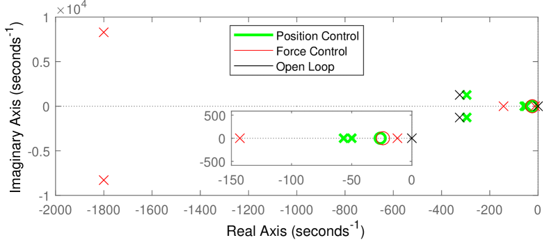
Figure 2: Pole-zero diagram of closed-loop controls versus plant

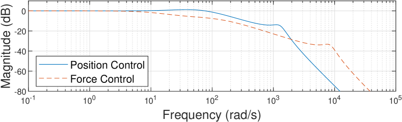
Figure 3: Bode diagram of designed closed-loop controls

The dominant poles, i.e. closer to origin, refer to the controlled actuator system dynamics. The gains were chosen so that no complex pole pairs occur close to the origin, and the most right real pole satisfies the requirements on the control system dynamics. In addition, higher gain values were avoided by taking into account the control saturations and measurement noise included into numerical simulation. From the Bode plot shown in Fig. 3, it can be seen that the first corner frequency, correspondingly bandwidth, is about 21Hz for the position control and about 2.5Hz for the force control. The determined control gains are listed in Table I.

TABLE I: Control gain parameters

	Position Control	Force Control
$K_{1}$	190	$0$
$K_{2}$	$9.019e^{-4}$	$2.5e^{-4}$
$K_{3}$	$30.539e^{-9}$	$5.9e^{-8}$
$K_{4}$	$0$	$5e^{-5}$
$K_{i}$	$5000$	$1.2e^{-3}$

Note that $K_{4}$ is set to zero for the position control and $K_{1}$ is set to zero for the force control, since these states are irrelevant for the respective control mode.

III-C Stability analysis

Generally it is desirable to proof a system to be globally stable. For physical systems that is in most cases however not feasible due the physical restrictions of the experimental setup which in this case are e.g. maximum pressure, range of motion of piston stroke, etc. Instead it can be pursued to proof the stability of the reachable state space. In this paper the proof of stability is limited to a subset of the reachable state space proofing local stability, specific for the test scenarios derived, due to spacial limitations. The local stability analysis relies on the stability of both linearized closed-loop control systems, see poles configuration in Section III-B, and multiple Lyapunov function approach applicable to the switched systems, see [17]. Note that the stability of switching between the motion and force control has been recently discussed in detail in [16], that for the linearized closed-loop behavior and autonomous switching by means of a hysteresis relay. Thus, we give here the main statement only, while for details on using the multiple Lyapunov function an interested reader is referred to [17] in general and to [16] for the motion and force control systems more specifically. For both closed-loop control systems, given by (6), the quadratic Lyapunov function candidate can be assumed as

$$L(h)=W_{1}\dot{x}^{2}+W_{2}P_{L}^{2}+W_{3}\bigl{(}r(h)-y(h)\bigr{)}^{2}.$$ (15)

Note that this contains all terms related to an energy storage in the control system: kinetic energy of the relative motion, potential energy of hydraulic pressure and potential energy of the feedback control loop reflected through the quadratic control error. The positive coefficients $W_{1-3}$ can be found for Lyapunov stability proof and used as mode-dependent, i.e. $W_{i}(h)$, that for the sake of better visualization/comparison of the multiple Lyapunov function. A non-increase in the Lyapunov function level for two consecutive operations of the same mode implies the entire switched system is asymptotically stable, cf. [16], in this case meaning an alternating position and force control mode. Since both closed-loop dynamics are linearized and stable in vicinity to the switching point, the above local stability of the switching between the modes appears sufficient for analysis of the designed hybrid control system and its test scenarios.

IV Experimental Evaluation

An experimental evaluation of the proposed hybrid control is given below. The laboratory view of the experimental setup is shown in Fig. 4 while for more details the reader is referred to [14].

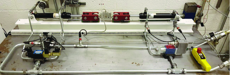
Figure 4: Experimental setup of hydraulic actuators

Two test scenarios are considered: in the first one the controlled motion of the piston rod of the right-hand cylinder is executed until hard-stop at the cylinder boundary. In the second one a slow dynamic counteracting force is introduced during which the piston rod is moving within $0\leq x<l$, since a hydraulic actuator is unsuitable for high dynamic force control applications [18]. The counteracting force is produced by another (left-hand) cylinder connected to the bidirectional control valve (BDCV), which changes the flow direction, and pressure relief/reduction valve (PRV), to adjust pressure. This allows producing an adjustable (open-loop controlled) force on the stiff interface between both cylinders. The supply pressure was set to $P_{S}=100e^{5}$ Pa, and flow to $40$ l/min.

IV-A Hard-stop environment

The controlled motion starts at zero position (controlled right-hand cylinder fully retracted) and follows the ramp reference with a slope corresponding to 0.03 m/s velocity, cf. Fig. 5. The controlled motion reaches hard-stop when the overall drive of both cylinders, connected stiffly, reaches mechanical boundary of the left-hand cylinder. Note that during the experiment the BDCV is in zero position, thus opening both chamber lines of the left-hand cylinder to the tank and, thus, providing no active counteraction force but passive additional load only. When reaching hard-stop by environment, the counteracting force rises, due to the stiff position control, and the hysteresis relay-based switching triggers the force control at the set threshold value. The force reference trajectory is initially set to the constant value $r(1)=3500N$ and afterwards decreases towards zero in a slow cosine shape. This reference trajectory is assigned in order to evaluate simultaneously the set value and trajectory following of the force control and, the autonomous switching back to the position control. The latter occurs when passing the lower threshold value of the load force, that means releasing from the contact with environment. After switching back, the position control tracks the negative ramp, with a slope corresponding to $-0.03$m/s velocity, that until reaching the initial zero position.

Figure 5 shows the reference and measured position values of the right-hand cylinder rod. The transient phases at the beginning of relative motion and after switching back (from the force to position control) are additionally zoomed-in around the time of 0.1 sec and 8.5 sec correspondingly. Accurate reference following with solely minor transient overshoots can be recognized.

Figure 5: Reference and measured position control response

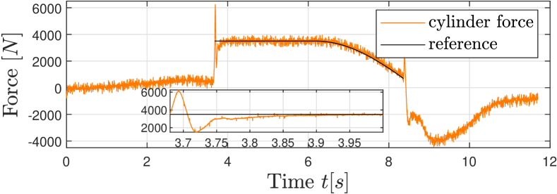
Figure 6: Reference and measured force control response

Figure 6 shows the sensor measured counteraction force versus the corresponding reference. Note that the triggered force control is active only during the time span where the reference is indicated, while the residual force measurements correspond to both slopes of the controlled motion, i.e. position control. There, the load force occurs between the right-hand (driving) cylinder and left-hand (driven) cylinder. An accurate force following can be recognized, while some transient swinging occurs at the hard-stop contact, which is an inherent and well-known issue of the force control in general, compare with e.g. [7, 10].

In order to assess repeatability of the proposed hybrid control scheme, a total of 20 experiments were conducted. The mean values and standard deviations of the control errors are evaluated from the signals processed by the second-order LPF with 100 Hz cutoff frequency. The low-pass filtering is done for the sake of better visualization of all tests against each other, since the inherent level of process and measurement noise in the hydraulic system is relatively high. Figures 7(a) and 7(b) show the absolute mean values and standard deviations of the position control error for both ramp segments of the rod displacement. The absolute mean values and standard deviations of the force control errors are shown in Fig. 8.

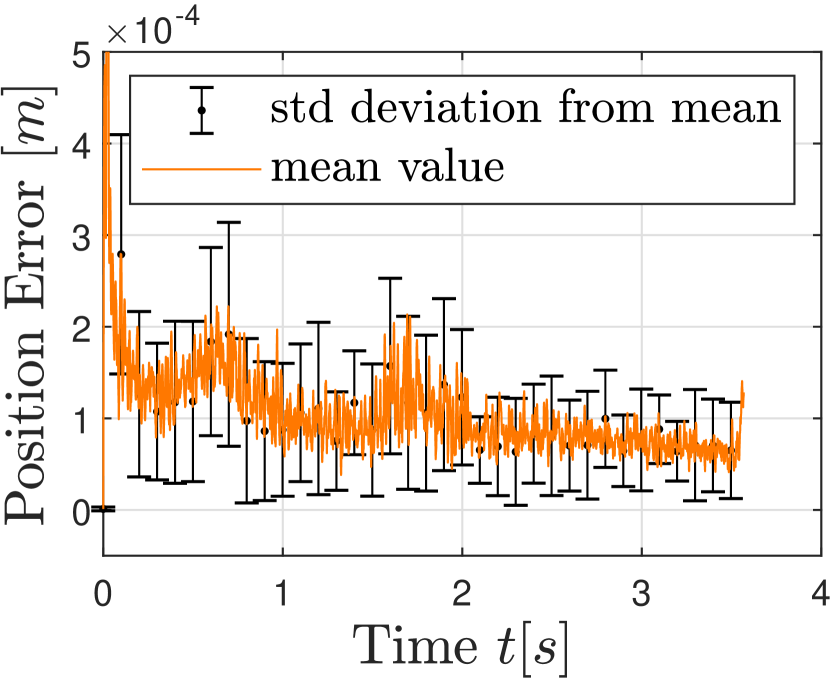
(a) extending

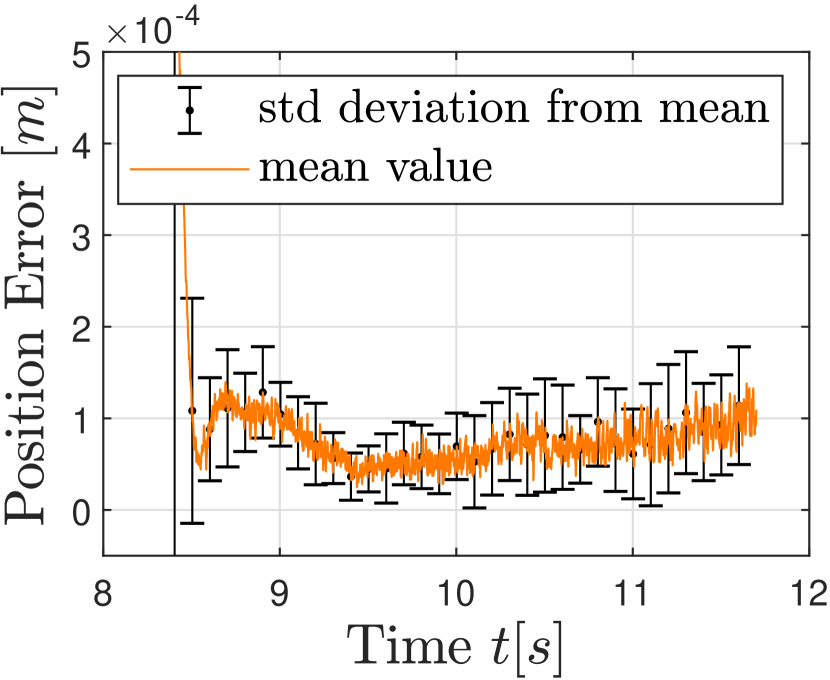
(b) retracting

Figure 7: Position control error over 20 experiments

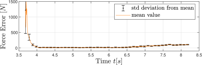
Figure 8: Force control error over 20 experiments

IV-B Dynamic environment

For the test scenario with dynamic environment, the controlled motion starts at fully retracted zero position, following a ramp reference within first 1.5 sec, after which the reference trajectory becomes a slow sinusoidal pattern, cf. Fig. 9. Note that the reference trajectory $r(-1)$ is shown for the position control mode only; after switching back from the force control, the position reference is recalculated on the fly. The left-hand cylinder is feed-forward controlled in an open-loop manner, while being stiffly coupled to the right-hand (controlled) one. This way, a varying counteraction force is generated. The BDCV control value, for the left-hand cylinder, is chosen such that it is continuously driving the left-hand cylinder, while the PRV is controlled in a pulsed pattern with 10 sec period and 60% pulse-width. The force reference trajectory $r(1)$ starts at 3375 N and then steps up and down to 4500 N and 3150 N respectively, see Fig. 10. These step values are chosen such that the controlled cylinder rod cannot reach fully extended/retracted states while pushing against the left-hand cylinder rod. Figure 9 shows the position measurement together with the reference trajectory segments. After 4 sec time, labeled by the dashed bar, the PRV controlling the left-hand load cylinder switches to high, thus resulting in an increased load force and, hence, triggering switch to the force control mode.

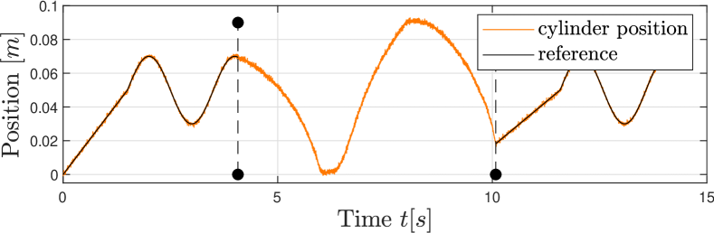
Figure 9: Reference and measured position control response

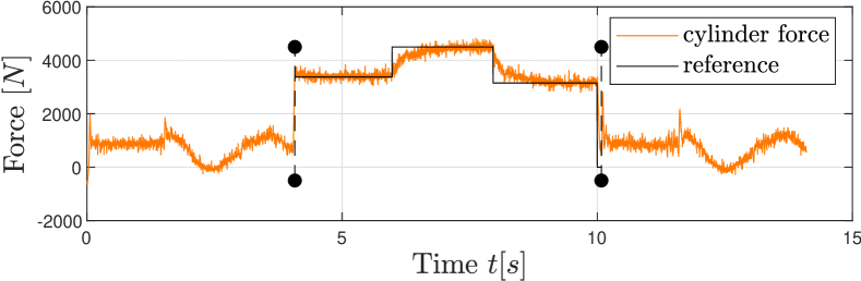
Figure 10: Reference and measured force control response

The corresponding reference force and (all time) measured load force can be seen in Fig. 10. After 10 sec time, the PRV control value is again at low-level, the load force drops below the relay switching threshold and the hybrid controller changes back to the position control mode, labeled by the second dashed bar in Fig. 10. Note that between both dashed bars, a relative motion occurs (see Fig. 9), while the required controlled force is kept constant, cf. Fig. 10. Also here the experiments were repeated 20 times, while the same signals filtering as described above was applied when evaluating the absolute mean values and standard deviation of the control error. Both are shown in Figs. 11(a) and 11(b) for the position control mode, and in Fig. 12 for force control mode respectively.

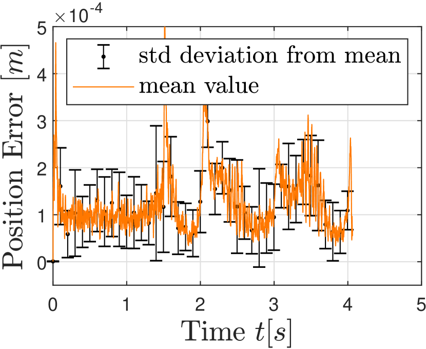
(a) initial

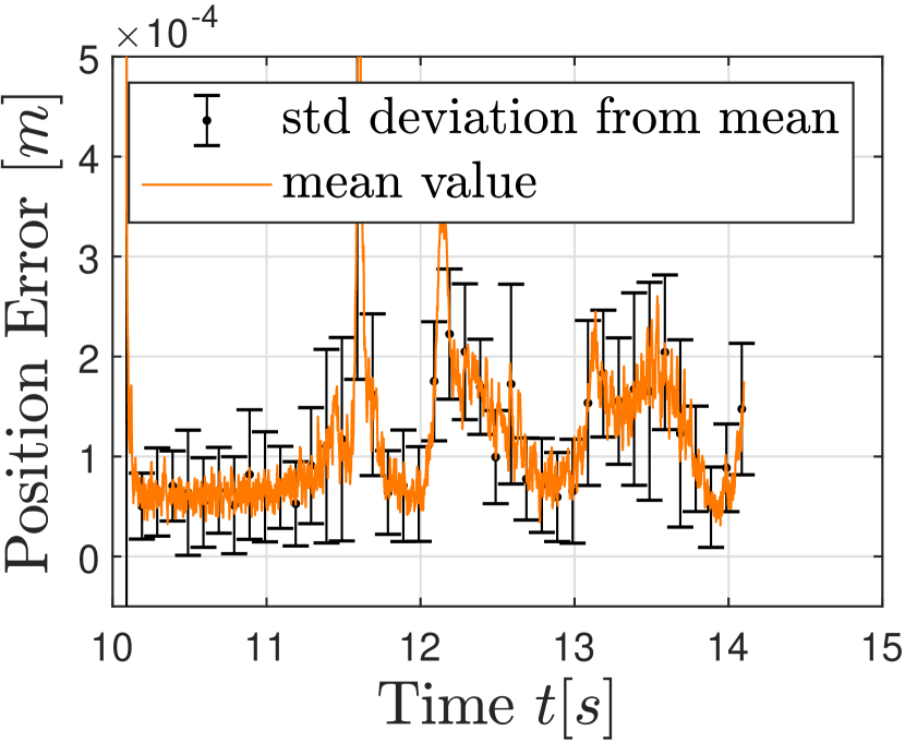
(b) last

Figure 11: Position control error over 20 experiments

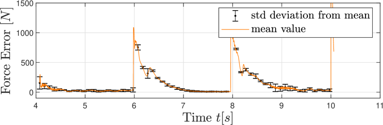
Figure 12: Force control error over 20 experiments

V Summary

A novel hybrid position/force control suitable for standard linear-stroke hydraulic actuators was proposed. For its development an experimental hydraulic test rig with two cylinders in antagonistic setup was designed, assembled, and instrumented. The corresponding full-order model of the system was derived. A reduction of the state-space model was made, forming basis for the hybrid control loop design. The included autonomous switching between the position and force control relies on the hysteresis relay, that without changing the overall control structure. Control parameters were obtained based on the pole placement. The local stability around the operation and switching points was shown. Two experimental studies were illustrated for evaluating the repeatability and performance of both, position and force controls, and switching between them.

References

- [1] M. Jelali and A. Kroll, Hydraulic Servo-systems : Modelling, Identification and Control. Springer London, 2003.
- [2] H. E. Merritt, Hydraulic control systems. John Wiley and Sons, 1967.
- [3] G. Liu and S. Daley, “Optimal-tuning nonlinear PID control of hydraulic systems,” Control Engineering Practice, vol. 8, no. 9, pp. 1045–1053, 2000.
- [4] S. Koch and M. Reichhartinger, “Observer-based sliding mode control of hydraulic cylinders in the presence of unknown load forces,” Elektro- und Informationstechnik, vol. 133, no. 6, pp. 253–260, 2016.
- [5] C. Vazquez, S. Aranovskiy, L. Freidovich, and L. Fridman, “Second order sliding mode control of a mobile hydraulic crane,” in 53rd IEEE Conference on Decision and Control, 2014, pp. 5530–5535.
- [6] Bin Yao, Fanping Bu, J. Reedy, and G.-C. Chiu, “Adaptive robust motion control of single-rod hydraulic actuators: theory and experiments,” IEEE/ASME Trans. on Mechatronics, vol. 5, no. 1, pp. 79–91, 2000.
- [7] A. Alleyne and R. Liu, “A simplified approach to force control for electro-hydraulic systems,” Control Engineering Practice, vol. 8, no. 12, pp. 1347–1356, 2000.
- [8] J. Komsta, N. van Oijen, and P. Antoszkiewicz, “Integral sliding mode compensator for load pressure control of die-cushion cylinder drive,” Control Engineering Practice, vol. 21, no. 5, pp. 708–718, 2013.
- [9] N. Niksefat and N. Sepehri, “Design and experimental evaluation of a robust force controller for an electro-hydraulic actuator via quantitative feedback theory,” Control Engineering Practice, vol. 8, no. 12, pp. 1335–1345, 2000.
- [10] S. Katsura, Y. Matsumoto, and K. Ohnishi, “Analysis and experimental validation of force bandwidth for force control,” IEEE Transactions on Industrial Electronics, vol. 53, no. 3, pp. 922–928, 2006.
- [11] M. H. Raibert and J. J. Craig, “Hybrid Position/Force Control of Manipulators,” Journal of Dynamic Systems, Measurement, and Control, vol. 103, no. 2, p. 126, 1981.
- [12] O. Khatib, “A unified approach for motion and force control of robot manipulators: The operational space formulation,” IEEE Journal on Robotics and Automation, vol. 3, no. 1, pp. 43–53, 1987.
- [13] M. Ruderman, “Full- and reduced-order model of hydraulic cylinder for motion control,” in 43rd Annual Conference of the IEEE Industrial Electronics Society, 2017, pp. 7275–7280.
- [14] P. Pasolli and M. Ruderman, “Linearized Piecewise Affine in Control and States Hydraulic System: Modeling and Identification,” in Linearized Piecewise Affine in Control and States Hydraulic System: Modeling and Identification. IECON2018 - 44th Annual Conference of the IEEE Industrial Electronics Society, 2018, p. 8.
- [15] ——, “Hybrid State Feedback Position-Force Control of Hydraulic Cylinder,” in 2019 IEEE International Conference on Mechatronics (ICM), 2019, pp. 54–59.
- [16] M. Ruderman, “On switching between motion and force control,” in 27th Mediterranean Conference on Control and Automation, MED 2019 - Proceedings. Institute of Electrical and Electronics Engineers Inc., jul 2019, pp. 445–450.
- [17] D. Liberzon and A. Morse, “Basic problems in stability and design of switched systems,” IEEE Cont. Syst., vol. 19, no. 5, pp. 59–70, oct 1999.
- [18] A. Alleyne and R. Liu, “On the limitations of force tracking control for hydraulic servosystems,” Journal of Dynamic Systems, Meas. and Cont., Trans. of the ASME, vol. 121, no. 2, pp. 184–190, jun 1999.