Planning of School Teaching during COVID-19.

Abstract

More than one billion students are out of school because of Covid-19, forced to a remote learning that has several drawbacks and has been hurriedly arranged; in addition, most countries are currently uncertain on how to plan school activities for the 2020-2021 school year; all of this makes learning and education some of the biggest world issues of the current pandemic. Unfortunately, due to the length of the incubation period of Covid-19, full opening of schools seems to be impractical till a vaccine is available. In order to support the possibility of some in-person learning, we study a mathematical model of the diffusion of the epidemic due to school opening, and evaluate plans aimed at containing the extra Covid-19 cases due to school activities while ensuring an adequate number of in-class learning periods.

We consider a SEAIR model with an external source of infection and a suitable loss function; after a realistic parameter selection, we numerically determine optimal school opening strategies by simulated annealing. It turns out that blended models, with almost periodic alternations of in-class and remote teaching days or weeks, are generally optimal. Besides containing Covid-19 diffusion, these solutions could be pedagogically acceptable, and could also become a driving model for the society at large.

In a prototypical example, the optimal strategy results in the school opening $90$ days out of $200$ with the number of Covid-19 cases among the individuals related to the school increasing by about $66\%$, instead of the about $250\%$ increase that would have been a consequence of full opening.

1 Introduction

More than one billion students are out of school because of Covid-19 [1]; most of them are now using remote learning practices that present several drawbacks [2] and in most cases have been hurriedly arranged.

In addition, in most countries there is uncertainty on how to plan school activities for the 2020-2021 school year [3]. As a result, learning and education are two of the biggest world issues of the current pandemic [4, 5]. Unfortunately, due to the length of the incubation period of Covid-19 of about $5$ days [Qun2 et al. 020, Kai-Wang et al. 2020], full opening of schools seems to be impractical till a vaccine is available; this has been experienced by the first experiments of reopening [6, 7], and it is further confirmed by the simulations in the present paper.

In order to support the possibility of some in-person learning, we study a mathematical model of the diffusion of the epidemic due to school opening. More specifically, we consider an adaptation of the SEIR model to the problem of planning school teaching during the school year 2020-2021, when the COVID-19 epidemic is very likely to still be active. The aim is to optimize the number of in-class teaching days vs. remote ones in a school setting, while containing the number of extra infectious transmissions due to opening of the school.

To this purpose, we set-up a suitable system of ordinary differential equations describing the evolution of the epidemic among the personnel and the students of a school. The model, in analogy to SEIR, has susceptible individuals (S) to whom the virus can be transmitted either from external sources (when they are not at school), or from contacts with other individuals within the school. Susceptible individuals become pre-symptomatic or, equivalently, exposed (E) at transmission, entering a latency period in which they are already contagious; they then either show symptoms (I), or remain asymptomatic (A); both situations resolve, and individuals recover (R). As numbers are limited, and COVID-19 mortality is particularly low among young individuals, we disregard mortality. The key differences with the usual SEIR model [Chowell et al. 2009] are: an external source of infection [Naji2014], [Banerjee2014], the possibility of transmission limited to $7$ hours per working day, a control allowing preventative closure of the school each day, and the presence of asymptomatic individuals. The asymptomatic members of the community present a challenge, as they cannot be easily detected while still being infectious for a relatively long time: we assume accessibility to some type of fast screening with a minimal sensitivity [Wyllie2020].

We further assume that the objective of the planner is to maximize the number of days with in-class vs. remote teaching, and simultaneously minimize the number of extra infectious transmissions due the opening of the school. For this, it is essential that the planner determines the relative weight $\tau$ of these two objectives, but our set-up applies to any possible value of $\tau$. Once a value of $\tau$ is fixed, the aim of the planner becomes then to minimize a functional that combines these two objectives by the relative weight. To achieve her/his targets, the planner can decide ahead of time which days are in-class and which are restricted to remote teaching; for simplicity, we consider here a plan for the whole year, but monitoring and en route adjustments can be also incorporated. We remain agnostic as to the value of the relative weight $\tau$, and develop tools to analyze all possible scenarios.

We start from a careful evaluation of all the parameters of the model, except $\tau$, and for each scheduling plan we numerically evaluate the loss functional. We repeat this for random selections of the scheduling plans, obtaining a numerical description of the distribution of the outcomes in terms of remote days and additional infectious transmissions. In addition, for each value of $\tau$, we use simulated annealing to optimize with respect to weekly openings or closures. A model sensitivity analysis is then carried out to assess the effect of parameter evaluation errors. This gives a complete picture of the potentialities of the optimization procedure.

As we assume an external source of infection, a fraction of the individuals related to the school gets infected even with complete closure and remote only teaching. In a prototypical simulation, $12.2\%$ of the individuals are subject of an infectious transmission during the school year from contacts outside the school; they become pre-symptomatic or, as we indicate them, exposed (E). Recall that in our model, exposed individuals have received an infectious transmission; according to current estimates [Nishiura2020], about half of the exposed individuals develop symptoms (I). On the other hand, if the teaching is completely in-class, about $42.9\%$ of the individuals get the virus: that is almost half of the school population, and an increment of $251.63\%$ with respect to completely remote. The outcome of the optimization procedure depends on the relative weight $\tau$, but most optimal solutions turn out to be blended, with periodic alternations between weeks of in-class activities, and weeks of remote teaching: solutions of this type have been advocated and are being planned in Scotland [5]. In one such solution, there are $90$ days of in-class teaching, with the additional infectious transmissions contained to $7.9\%$, which is an increase of $64.75\%$ of the cases with respect to remote only activity. In a school of $1000$ individuals this corresponds to creating an extra $79$ cases of COVID-19 patients, next to the $122$ who would have been infected in any case; considering that about half of the cases are asymptomatic, this corresponds to having about $40$ extra symptomatic cases in exchange for almost half of the year spent in class. The administrators can decide to realize a stricter or more relaxed containment of the extra cases by assigning more or less weight to infectious transmissions. The solution to achieve the above results is (0, 0, 0, 1, 0, 1, 0, 0, 0, 1, 0, 1, 0, 1, 0, 1, 0, 1, 0, 1, 0, 1, 0, 1, 0, 1, 0, 1, 0, 1, 0, 1, 0, 1, 0, 1, 0, 1, 0, 1), where $0$ indicates a week of remote, and $1$ a week of in-class activities; notice that there is an initial period of closure, before progressing to a regular alternation of openings and closures. If $18$ out of the $40$ weeks are open at random, the same number of in-class days as above but with no plan, then the increment in the number of cases is $88\%$ on average, with a Standard Deviation of $10.25\%$: making an random selection of the weeks of in-class activities would thus result in a substantial reduction of the number of extra infections; on the other hand, the optimal solution is statistically better, as it is more than $2$ SD’s below what the average random selection would provide, and it is also not subject to possible adverse fluctuations.

In Section 3 we carry out a sensitivity analysis, which shows that the optimal planning is pretty stable in case of some extra opening or remote days, and is only moderately affected by errors in parameter selection, within certain ranges. The most significant parameters are the infectious rate for contacts in the school $\beta$, the duration of the incubation period before symptoms are developed $1/\gamma$, and the capability of screening for asymptomatic individuals $\eta$. Our results are acceptable if the incubation period is below $7$ days on average: while current estimation give about $5$ days [Qun2 et al. 020, Kai-Wang et al. 2020], this parameter needs to be monitored from the evolving studies. In this study, we take the infectious rate for contacts in the school at a much higher than all current estimates, but since a school is a densely populated environment, precautions and distancing methods must applied as much as possible not to overcome even our pessimistic selection. For the fraction of detected asymptomatic individuals, we assume that this is at least $45\%$: this fraction relies on testing, that should then be performed regularly, possibly with simple and inexpensive, even if not totally reliable, methods [Chekani-Azar2020].

Related studies. Optimization methods similar to those used in this paper have appeared in many other contexts. In fact, several recent studies have considered optimal planning strategies in response to general epidemics [Chowell et al. 2009, Jones2020] or, more specifically, to the COVID-19 pandemic [alvarez2020, Grigorieva2020]; to our knowledge, however, none has considered the current optimization problem for school planning.

Limitations. There are several limitations to this study. Our results are only a first indication of a modeling methodology for the search of an optimal trade off between in-class teaching and containment of infectious transmissions. Even if parameters are carefully and realistically selected, the values are based on information known at the time of this study; when a parameter has a wide range of variability we settle for one representative value; in addition, the worked out examples referred to an ideal school: for each particular concrete situation, one needs to adapt the model to the specific case.

We also did not consider other alternatives, such as having half of the classes, or reducing the number of in-class students for each class. These alternatives could be conveniently incorporated in a more elaborate model.

2 A SEAIR model with external source and containment

2.1 Epidemic model

We consider SEAIR, a version of the SIR model [Chowell et al. 2009] with an external source of infection [Naji2014, Blackwood2018], and a control. The population is divided into: susceptible (S), pre-symptomatic or, equivalently, exposed (E), asymptomatic (A), infected (I) and recovered (R). Variables are normalized so that $S+E+A+I+R=1$.

We assume that susceptible individuals might become exposed (E), a phase in which they have contracted the virus and are contagious, without showing symptoms. The contagion can be caused by contact with other individuals with viral load, at a rate $\beta c(t)$ ($c(t)$ is the control, as described below); or, alternatively, it is caused by an infectious contact outside the school taking place at rate $\alpha$. Exposed individuals either develop symptoms at a constant rate $\delta$, becoming infected, or progress into being asymptomatic with rate $\gamma$. The viral load is carried by exposed (E), asymptomatic (A) or infectious (I) individuals; however, infectious individuals are assumed to be isolated, while a large fraction of asymptomatic (A) is supposed to be detected; hence, if the school is open then susceptible individuals are assumed to enter in contact only with exposed, and a fraction $\eta$ of asymptomatic.

Both asymptomatic and infected individuals recover at rate $\rho$.

With these assumptions, the system of OdE modeling infectious transmissions of concern for the school is:

$$\text{Susceptible:\quad}\frac{dS}{dt} =-\alpha S-\beta Sc(t)(E+\eta A)$$ (1)

$$\text{Exposed:\quad}\frac{dE}{dt} =\beta Sc(t)(E+\eta A)+\alpha S-(\gamma+\delta)E$$ (2)

$$\text{Asymptomatic:\quad}\frac{dA}{dt} =\gamma E-\rho A$$ (3)

$$\text{Infected:\quad}\frac{dI}{dt} =\delta E-\rho I$$ (4)

$$\text{Recovered:\quad}\frac{dR}{dt} =\rho(A+I)$$ (5)

for a certain time interval $[0,T]$. We consider $40$ weeks, and count time in hours, so that $T=6720$. The initial population at the beginning of the school year might be partly immune due to previous infections, but to avoid questions about efficacy and duration of the immunity, we assume that the initial population consists primarily of susceptible, $S(0)\approx 1$, and a small fraction of exposed, so that $S(0)+E(0)=1$.

The function $c(t)$ describes the control variable, and it is $c(t)=0$ for all times when the school is closed; these include all hours except the opening times. For each of the $200$ working days, $c(t)$ can be $0$ again if remote activities have been decided for that day, or $1$ if teaching is in person. Formally, with $t$ measured in hours, let $\mathcal{M}$ indicate the class of controls $c(t)$ such that

$$c(t)=\begin{cases}c_{i,j}\quad\text{ if }i=\lfloor t/168\rfloor,j=\lfloor(t-168\lfloor t/168\rfloor)/24\rfloor\leq 5\quad\text{ and }\\ \quad\quad\quad 8\leq t-168\lfloor t/168\rfloor-24\lfloor(t-168\lfloor t/168\rfloor)/24\rfloor\leq 15\\ 0\quad\text{ otherwise }\end{cases}$$ (6)

for some $c_{i,j}\in\{0,1\},i=1,\dots,40,j=1,\dots,7$, and $0\leq t\leq 6720.$

2.2 Mathematical analysis

Lemma 2.1.

For each solution of (1)-(5), the total population $S+E+A+I+R$ is preserved.

Proof.

If $\vec{X}(t)=(S(t),E(t),A(t),I(t),R(t))$ is a solution, then let $\phi=S+E+A+I+R$; we have that $\phi(0)=1$ and $\frac{d\phi}{dt}=\frac{d(\phi-1)}{dt}=-n(\phi-1)$, so that, since $(\phi-1)(0)=0$, necessarily $\phi\equiv 1$ by uniqueness of solutions of linear differential equations. ∎

Notice that, in addition, $0\leq S,E,A,I,R\leq 1$.

Lemma 2.2.

For all initial conditions $\vec{X}(0)=(S(0),E(0),A(0),I(0),R(0))$ such that $0\leq S(0),E(0),A(0),I(0),R(0)\leq 1$ there exists a unique solution of the system (1)-(5) for all times.

Proof.

Since $c(t)\in\{0,1\}$ and $S,E,A,I,R$ are bounded, the r.h.s. of the system (1)-(5) is Lipschitz [Adkins12] in the variables $S,E,A,I,R$: in fact, let $\vec{F}(c,\vec{X})$ be the vector-valued function having as components the right-hand sides of the S-E-A-I-R-D differential equations; we can then rewrite the system in vector form

$$\vec{X}^{\prime}=\vec{F}(c,\vec{X}),\,\,\vec{X}(0)=\vec{X}^{0}.$$

We have that $\frac{\partial\vec{F}_{i}}{\partial\vec{X}_{j}}\leq c_{1}\max_{1\leq i\leq 5}\left\{\max_{[0,T]}|X_{i}(t)|\right\}\leq c_{1}$ for some $c_{1}>0$. This is a sufficient condition for existence and uniqueness of solutions in each interval of continuity of $c(t)$ [Adkins12]. As $c(t)$ has only jump discontinuities, the unique solution of an interval can be uniquely continued as a continuous function into the next interval [Adkins12]; hence there always exist a unique solution for all times $t$ of the system (1)-(5). ∎

Lemma 2.3.

If $(S(0)+E(0)+A(0)+I(0)+R(0))=1$ then there is a unique stationary solution, namely $S=E=A=I=0,R=1$, which then attracts the solution for all initial conditions.

Proof.

For a stationary solution, $\vec{X}^{\prime}=0$ implies $S=0$ by (1). Then, (2) implies $E=0$, and (3)-(4) imply $A=I=0$. By Lemma 2.1, it must then be $R=1$. ∎

We are, however, interested in a finite time interval $T$, and hence in the transient solution up to time $T$.

2.3 Planner’s objectives

The planner’s objectives are incorporated in the model by a loss function, defined as follows. One of the aims of the planner is to contain the number of extra infectious transmissions due to the opening of the school; let $S_{0}(t)$ be the fraction of susceptible with completely remote teaching, that is with $c\equiv 0$, at time $t$; $S_{0}(0)-S_{0}(T)$ is then the fraction of individual who receive an infectious transmission even if the school never opens; then, let $S(t)=S_{c}(t)$ be the fraction of susceptible with opening plan $c(t)$; we have that $S_{0}(T)-S(T)=S_{0}(T)-S_{c}(T)=(S_{c}(0)-S_{c}(T))-(S_{0}(0)-S_{0}(T))$ is the fraction of extra infectious transmissions due to the opening of the school according to plan $c(t)$. In addition, let $N(c)=400-\intop_{0}^{T}c(t)dt/7$ be the number of remote teaching days (the factor $1/7$ is due to the number of hours that the school is open in a regular day). The loss function combining the two effects is then

$$\mathcal{L}=(S_{0}(T)-S(T))+(N(c)/\tau)$$

where $\tau$ is the relative weight of a day of in-class teaching to infectious transmissions: $\tau/100$ can be interpreted as the number of days of in-class teaching that the planner considers equivalent to a $1\%$ increase in the infectious transmissions in the school.

The planner’s objective becomes then

$$\min_{c\in\mathcal{M}}\mathcal{L}$$ (7)

with $\mathcal{M}$ as in (6). It is easy to see that using the system (1)-(5) the optimization problem can be cast in a more standard form [Fleming75, Grigorieva2020], in which

$$\mathcal{L}=E_{c}(T)-E_{0}(T)+\int_{0}^{T}\left((\gamma+\delta)(E_{c}(t)-E_{0}(t)+\frac{1}{7\tau}c^{2}(t)\right)dt$$

where $E_{0}(t)$ is the exposed component of the solution of the system (1)-(5) for the case $c\equiv 0$; however, as we optimize over the very restricted class of functions (6), which are piecewise constant and depend on the finite number of parameters $c_{i,j}$’s, the general theory of control optimization is not needed here: (7) becomes a discrete optimization problem.

3 Simulations

3.1 Parameter selection

We select the epidemic parameters based on current observations. As time is counted in hours, we need to scale all available estimates, usually expressed in days, by a factor of $24$.

There is a large variability in the estimations of the COVDI-19 infection rate $\beta$, with estimated values tipically around $0.25$-$3$ [Toda2020]; however, as the school is likely to elicit more frequent contacts, we adopt a fairly higher value of $\beta=0.9/24\approx 3.75\times 10^{-2}$.

Duration of the latency period after infection and before symptoms are developed has been estimated in about $5$ days (see for example [Qun2 et al. 020] and [Kai-Wang et al. 2020]), so that $\gamma+\delta\approx 1/5\times 1/24=0.2/24$; the fraction of asymptomatic is also quite problematic, with estimates ranging from $5\%$ to $60\%$, we adopt a value of $50\%$, slightly higher than the average [Nishiura2020]; therefore, we take $\gamma=\delta=0.1/24\approx 4.17\times 10^{-3}$. Similarly, the average recovery period is about $7$ days, for mild cases [Byrne et al. 2020], suggesting $\rho=0.14/24\approx 5.8\times 10^{-3}$; more severe cases (I) are excluded from contacts, so their recovery rate is irrelevant: we use the same value of $\rho$.

The parameter $\eta$ describes how asymptomatic individuals are excluded from contacts with the other individuals; such a separation depends on the availability of detecting tests: we assume that a sufficiently reliable test is available, with a $90\%$ test sensitivity, so that $\eta=0.1$. This assumption is subject to parameter sensitivity analysis in Section 3 below, where we see that a test sensitivity of at least $45\%$ is needed for our calculations to make sense.

We finally consider the external rate of infection. At this moment, countries, with few exceptions, have reported at most $1\%$ of infected, but data is not considered reliable [Verity et al. 2020]; we take an external infection rate $\alpha\approx 1.78\times 10^{-5}$ such that in the observation period of $40$ weeks there is a moderate, but non negligible number of cases even with the school being totally closed; with our selection of parameters the individuals infected outside of the school will be about $12.2\%$ of the total. The parameter $\alpha$ will be carefully monitored in the sensitivity analysis, but its value is seen to be irrelevant to our conclusions.

Table 1: Recap of the model parameters and their estimated values.

Parameter	Selected value
$\alpha$	$1.78\times 10^{-5}$
$\beta$	$3.75\times 10^{-2}$
$\gamma$	$4.17\times 10^{-3}$
$\delta$	$4.17\times 10^{-3}$
$\rho$	$5.83\times 10^{-3}$
$\eta$	$0.1$

As initial condition, we assume that there are a few exposed individuals already present at the start of the school year, so we start from $E(0)=0.01$

3.2 Results

For simplicity, we have assumed here that the decision about remote or in-class teaching is taken for each week, so the control $c_{i}=c_{i,j}$ depends only on $i=1,\dots,40$. This still includes $2^{40}$ possible policies.

With the parameters as in Table 1, Column $2$, we have optimized by Simulated Annealing [Kirkpatrick83] as follows. First we have selected one value of $\tau$; we have taken the range $\tau\in[0.5,2000]$, this corresponds to between $0.5$ and $20$ days of in-class teaching rated equivalent to a $1\%$ increase in the number of infected; for each value of $\tau$, we have selected a random vector $v\in\{0,1\}^{40}$, and then, starting from the policy $c_{i}=v_{i}$, we have optimized by Simulated Annealing. Figure 1 shows a plot of fraction of infected vs. days of closure for each step of each simulation.

Figure 1: Fraction of infected vs days of remote teaching, several random combinations and optimal ones. The optimal once are close to the continuous curve. One special optimal solution in red

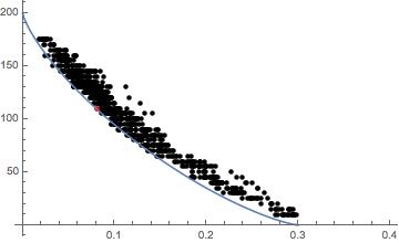
The optimal results for the various values of $\tau$ lie approximately on the curve $(\frac{x}{0.3})^{0.76}+(\frac{y}{200})^{0.76}=1$, which is also plotted in Figure 1. Points approximately on the curve correspond to the optimal policies for the various values of $\tau$. One can see the effect of optimization with respect to a random selection. The above curve is only numerically determined, and its significance is still unclear.

We have then selected one of the optimal policies, plotted in red in Figure 1. It corresponds to the following selection of open and closed weeks

$$\{0,0,0,1,0,1,0,0,0,1,0,1,0,1,0,1,0,1,0,1,0,1,0,1,0,1,0,1,0,1,0,1,0,1,0,1,0,1,0,1\},$$ (8)

in which $0$ stands for a week of remote teaching. Notice that the solution is quite periodic, with alternated weeks of in-class and remote activities; Figure 2 shows the evolution of the epidemic functions under the optimal policy (8).

Figure 2: Epidemic functions under the optimal policy (8). For visualization purposes, $E(t)$ is multiplied by $50$, and $A(t)$ and $I(t)$ are multiplied by $150$. Time is in hours.

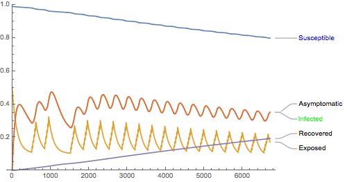
Table 2 summarizes the change in infectious transmissions with the optimal solution; notice that there is an increase of $64.75\%$ in the number of the positive cases due to the $90$ days of school opening vs. an increase of $251\%$ if the school was open all the $200$ days. This realizes an effective containment of the extra diffusion of the virus, while still having the possibility of offering a substantial portion of the teaching in person.

Table 2: Performance of optimal and random solutions with $90$ days of in-class teaching. First $4$ columns: total number of infectious transmissions; last $3$ columns: percentage increase with respect to remote only solution.

	Remote	Optimal	Random	In-class	Change w/: Optimal	Random	In-class
$\%$	$12.20$	$20.31$	$22.96\pm 1.25$	$42.93$	$64.75$	$88\pm 10.25$	$251.88$

We have also explored the possibility of selecting at random which weeks to open or close, with the constraint of having $90$ days of in-class activities. A simulation of the distribution gives then the increment in the number of cases is $88\%$ on average, with a Standard Deviation of $10.25\%$, hence the optimal solution is more than $2$ SD’s below what the average random selection would provide.

4 Sensitivity Analysis

We provide a two parts sensitivity analysis for our model.

The first part concerns errors in determination of the optimal solution. If one of the weeks for which remote teaching is planned by the optimal solution is instead changed into an in-class week, then the increment in the number of cases due to school opening ranges from an extra $70\%$ to an extra $76\%$, compared to the extra $66\%$ of the optimal solution. If one week is moved remote from in-class, then the increment in the number of cases is reduced to about $62\%$. If the planner had a value for each in-class day that lead to the solution with $90$ in-class days, altering the number of weeks of opening is not optimal, but it does not substantially change the final outcome: therefore, once an optimal policy has been determined, extra openings or closures can be adopted if needed without major changes in the final outcome. In addition, once the flexible blended model has been adopted, one can quickly and easily adapt to major changes in the external conditions, such as a sudden outbreak or a vaccine.

The second part of the sensitivity analysis concerns each of the parameters of the model used to determine the optimal solution (8). For each parameter, we compare the increase in the number of cases from the remote solution, and we contrast this with the increase for the complete in-class option. The results are reported in Table 3.

The last column of the table indicates the acceptable range of parameters: as the increase is $64.75\%$ if the selected parameters are correct (see Table 2), we accept up to a two-fold increase in the number of cases, which is a $100\%$, and report the resulting range.

Table 3: Sensitivity analysis. For each parameter, the second column gives the tested range; the third column indicates the change in number of cases compared to the change in case of full opening for the best value in the range; the fourth column indicates the worst case; the last column reports the acceptable range in which the number of cases doubles at the most.

parameter	test range	Minimal effect	Maximal effect	Accept. range
$\alpha$	$0.1\mbox{-}15\times 10^{-5}$	$16\%\text{ vs. }32\%\quad$	$71\%\text{ vs. }487\%$	$0.1\mbox{-}15\times 10^{-5}$
$\beta$	$0.1\mbox{-}10\times 10^{-2}$	$0.8\%\text{ vs. }2\%\quad$	$391\%\text{ vs. }664\%$	$0.1\mbox{-}5\times 10^{-2}$
$\gamma(=\delta)$	$0.1\mbox{-}10\times 10^{-3}$	$23\%\text{ vs. }64\%\quad$	$722\%\text{ vs. }722\%$	$3\mbox{-}10\times 10^{-3}$
$\rho$	$0.1\mbox{-}10\times 10^{-3}$	$63\%\text{ vs. }239\%\quad$	$224\%\text{ vs. }630\%$	$1\mbox{-}10\times 10^{-3}$
$\eta$	$0\mbox{-}1$	$60\%\text{ vs. }221\%\quad$	$139\%\text{ vs. }497\%$	$0\mbox{-}0.55$

We see that changes in the rate of external infections $\alpha$ does not alter the effectiveness of the optimal planning, as we always get a substantial reduction from full opening, and never more than $71\%$ increase; the range of $\alpha$ covers the possibilities that between $1.6\%$ and $64\%$ of the individuals of the school would be infected outside of the school even with complete closure; this covers all possible scenarios of evolution of the virus.

The internal transmission rate $\beta$ is, on the other hand, quite significant; if it goes above $5\times 10^{-2}\times 24=1.2$ then the number of cases would more than double due to the school opening: current estimates are around $0.3$, but this limitation indicates that one has to make sure that there are not too many occasions of infectious transmission within the school.

The incubation period before symptoms are developed $1/(\gamma+\delta)$ cannot exceed $\frac{1}{6\times 24}10^{3}\approx 7$ days on average, or else the number of cases would more than double with the optimal school activities: while this is now estimated to be $5$ days on average, one needs to monitor whether more accurate studies confirm this assessment.

The symptomatic period $1/\rho$ also is assumed to not exceed $\frac{1}{24}10^{3}\approx 41$ days on average, but this is a very safe bound.

Finally, the fraction of undetected asymptomatic $\eta$ must not exceed $55\%$: we assume availability of a easy, rapid and cheap test with a rate of false negative not exceeding $55\%$, such as CRISPR [Chekani-Azar2020].

5 Conclusions

We have considered the issue of planning in-class activities for the school year ’20-’21. Education is, in fact, one of the areas in which the measures to contain the current Covid-19 pandemic have hit the most, with many countries and local authorities struggling to find acceptable plans for next year.

To aid such planning, we have set up an optimization problem aimed at increasing the number of in-class vs. remote teaching, while containing the number of additional Covid-19 cases that would be determined by in-class school activities. The model involves differential equations to simulate the infectious transmissions, more precisely an SEAIR model with external source of infection and a control, a loss function combining the quantities to be minimized, and a numerical optimization procedure.

Our model has confirmed that the length of the incubation period of Covid-19 makes it impractical to have fully in-class activities: in a prototypical example, this would lead to an increase by more than $250\%$ of the Covid-19 cases among the individuals involved with the school.

We have then obtained a numerical expression for the curve of optimal strategies parametrized by the relative importance of in-class days vs. extra infectious transmissions. For a typical value of such relative importance, we have determined the optimal solution, which appears to be a blended model, with alternated weeks of in-class and remote teaching. The results turned out to be rather stable for possible errors in the estimation of model parameters, the more critical ones being the average incubation period, the internal transmission rate during school opening, and the fraction of detected asymptomatic individuals.

With the optimal strategy, the increase in the number of cases in the prototypical example, is around $66\%$. A random selection of the weeks of in-class teaching would be much less efficient, with an increase of about $88\%$ of the cases, but would still constitute a sharp reduction from full opening.

We think that this analysis, adapted to specific situations, could offer a very viable alternative for planning the school activities of the ’20-’21 school year. Some other aspects of socio-economic life could then be arranged around the blended model, in such a way that most children in the world will be able to enjoy an acceptable learning experience before a vaccine will hopefully allow the resumption of the usual school activities.

Contact address: NYU Abu Dhabi Saadiyat Island P.O Box 129188 Abu Dhabi, UAE

email: ag189@nyu.edu

References

- [1] [Unesco 2020-03-04] https://plus.google.com/+UNESCO (2020-03-04). ”COVID-19 Educational Disruption and Response”. UNESCO. Retrieved 2020-05-24.
- [2] [Unesco 2020-03-10] ”Adverse consequences of school closures”. UNESCO. 2020-03-10. Retrieved 2020-03-15.
- [3] [Unicef 20] What will a return to school during the COVID-19 pandemic look like? What parents need to know about school reopening in the age of coronavirus. Retrieved 2020-06-05,
- [4] [Ciano20] R. Cano: Prepping to reopen, California schools desperate for guidance, money. Calmatters, Retrieved 2020-01-05.
- [5] [Lyst 20] Coronavirus: What is a blended model of learning? By Catherine Lyst BBC Scotland, Retrieved 2020-01-05.
- [6] [Nelson et al. 20] Soraya Sarhaddi Nelson, Benjamin Restle and Monika M ller-Kroll: In Brief: COVID-19 outbreak leads city of G ttingen to shut schools through June 7, KCRW Berlin, Retrieved 2020-06-05.
- [7] [CBS 20] CBSNews: Coronavirus flare-ups force France to re-close some schools Retrieved 2020-05-18.
- [Chowell et al. 2009] Chowell, Gerardo and Hyman, James M and Bettencourt, Luís MA and Castillo-Chavez, Carlos: Mathematical and statistical estimation approaches in epidemiology. Springer (2009).
- [Naji2014] R K Naji, A A Muhseen: Modeling And Analysis Of An SVIRS Epidemic Model Involving External Sources Of Disease, INTERNATIONAL JOURNAL OF TECHNOLOGY ENHANCEMENTS AND EMERGING ENGINEERING RESEARCH, 2, 18 (2014), 2347-4289.
- [Banerjee2014] Banerjee, S., Chatterjee, A., AND Shakkottai, S: Epidemic thresholds with external agents, IEEE INFOCOM 2014-IEEE Conference on Computer Communications (2014), 2202?2210.
- [Wyllie2020] Wyllie, A.L. et al.: Saliva is more sensitive for SARS-CoV-2 detection in COVID-19 patients than nasopharyngeal swabs. medRxiv, Cold Spring Harbor Laboratory Press (2020), 2020.04.16.20067835.
- [Chekani-Azar2020] Chekani-Azar S, Gharib Mombeni E, Birhan M, and Yousefi M.: CRISPR/Cas9 gene editing technology and its application to the coronavirus disease (COVID-19), a review. J Life Sci Biomed 10, 1 (2020), 01-09.
- [alvarez2020] Alvarez, Fernando E and Argente, David and Lippi, Francesco: A simple planning problem for covid-19 lockdown. National Bureau of Economic Research, working paper 26981 (2020).
- [Blackwood2018] Julie C. Blackwood and Lauren M. Childs: An introduction to compartmental modeling for the budding infectious disease modeler Letters in Biomathematics 5, 1 (2018), 195-221.
- [Adkins12] Adkins, William A.; Davidson, Mark G.: Ordinary Differential Equations. Springer-Verlag, Berlin (2012).
- [Fleming75] W.H. Fleming and R.W. Rishel: Deterministic and Stochastic Optimal Control. Springer-Verlag, Berlin (1975).
- [Grigorieva2020] Grigorieva, Ellina and Khailov, Evgenii and Korobeinikov, Andrei: Optimal quarantine strategies for COVID-19 control models arXiv preprint arXiv:2004.10614 (2020).
- [Toda2020] Alexis Toda: Susceptible-infected-recovered (SIR) dynamics of Covid-19 and economic impact arXiv preprint: arXiv:2003.11221 (2020).
- [Qun2 et al. 020] Qun Li et al.: Early Transmission Dynamics in Wuhan, China, of Novel Coronavirus - Infected Pneumonia The New England Journal of Medicine 382 (2020), 1199-1207.
- [Kai-Wang et al. 2020] Kai-Wang et al.: Temporal profiles of viral load in posterior oropharyngeal saliva samples and serum antibody responses during infection by SARS-CoV-2: an observational cohort study. The Lancet Infectious Diseases 20 5 (2020), 565-574.
- [Nishiura2020] Nishiura, H.: Estimation of the asymptomatic ratio of novel coronavirus infections (COVID-19). International Journal of Infectious Diseases 94 (2020), 154-155.
- [Verity et al. 2020] Verity, Robert and Okell, Lucy C and Dorigatti, Ilaria and Winskill, Peter and Whittaker, Charles and Imai, Natsuko and Cuomo-Dannenburg, Gina and Thompson, Hayley and Walker, Patrick GT and Fu, Han et al.: Estimates of the severity of coronavirus disease 2019: a model-based analysis. The Lancet Infectious Diseases 20 6 (2020), 669-677.
- [Kirkpatrick83] Kirkpatrick, S. and Gelatt, C. D. and Vecchi, M. P.: Optimization by Simulated Annealing. Science 220 4598 (1983), 671-680.
- [Jones2020] Jones, Callum and Philippon, Thomas and Venkateswaran, Venky: Optimal Mitigation Policies in a Pandemic. Working paper (2020).
- [Byrne et al. 2020] Byrne et al.: Inferred duration of infectious period of SARS-CoV-2: rapid scoping review and analysis of available evidence for asymptomatic and symptomatic COVID-19 cases. medRxiv (2020).