Functional additive models for optimizing individualized treatment rules

Abstract

A novel functional additive model is proposed which is uniquely modified and constrained to model nonlinear interactions between a treatment indicator and a potentially large number of functional and/or scalar pretreatment covariates. The primary motivation for this approach is to optimize individualized treatment rules based on data from a randomized clinical trial. We generalize functional additive regression models by incorporating treatment-specific components into additive effect components. A structural constraint is imposed on the treatment-specific components in order to provide a class of additive models with main effects and interaction effects that are orthogonal to each other. If primary interest is in the interaction between treatment and the covariates, as is generally the case when optimizing individualized treatment rules, we can thereby circumvent the need to estimate the main effects of the covariates, obviating the need to specify their form and thus avoiding the issue of model misspecification. The methods are illustrated with data from a depression clinical trial with electroencephalogram functional data as patients’ pretreatment covariates.

Keywords: Individualized treatment rules; Functional additive regression; Sparse additive models; Treatment effect-modifiers

1 Introduction

We propose a flexible functional regression approach to optimizing individualized treatment decision rules (ITRs) where the treatment has to be chosen to optimize the expected treatment outcome. We focus on the situation in which potentially large number of patient characteristics is available as pretreatment functional and/or scalar covariates. Recent advances in biomedical imaging, mass spectrometry, and high-throughput gene expression technology produce massive amounts of data on individual patients, opening up the possibility of tailoring treatments to the biosignatures of individual patients from individual-specific data (McKeague and Qian, 2014). Notably, some randomized clinical trials (e.g., Trivedi et al., 2016) are designed to discover biosignatures that characterize patient heterogeneity in treatment responses from vast amounts of patient pretreatment characteristics. In this paper, we focus on some specific types of high-dimensional pretreatment patient characteristics observed in the form of curves or images, for instance, electroencephalogram (EEG) measurements. Such data can be viewed as functional (e.g., Ramsay and Silverman, 1997) and are becoming increasingly prevalent in modern randomized clinical trials (RCTs) as pretreatment covariates.

Much work has been carried out to develop methods for optimizing ITRs using data from RCTs. Regression-based methodologies are intended to optimize ITRs by estimating treatment-specific response (e.g., Qian and Murphy, 2011; Lu et al., 2011; Tian et al., 2014; Shi et al., 2016; Jeng et al., 2018; Park et al., 2020b; Petkova et al., 2020) while attempting to maintain robustness with respect to model misspecification. Machine learning approaches for optimizing ITRs are often framed as a classification problem (e.g., Zhang et al., 2012; Zhao et al., 2019), including outcome weighted learning (e.g., Zhao et al., 2012, 2015; Song et al., 2015) based on support vector machines, tree-based classification (e.g., Laber and Zhao, 2015) and adaptive boosting (Kang et al., 2014), among others. However, to date there has been relatively little research on ITRs that directly utilize pretreatment functional covariates. McKeague and Qian (2014) proposed methods for optimizing ITRs that depend upon a single pretreatment functional covariate. The flexible functional regression approach of Ciarleglio et al. (2016) is also restricted to a single pretreatment functional covariate. Ciarleglio et al. (2015) proposed a method allowing for multiple functional/scalar covariates, and extended to incorporate a simultaneous covariate selection for ITRs in Ciarleglio et al. (2018). However, both of these approaches are limited to a stringent linear model assumption on the treatment-by-covariates interaction effects that limits flexibility in optimizing ITRs and to two treatment conditions.

In this paper, we allow for nonlinear interactions between the treatment and the pretreatment functional covariates on the outcome and also for more than two treatment conditions. We incorporate a simultaneous covariate selection for ITRs through an $L^{1}$ regularization to deal with a large number of functional and/or scalar covariates. In a review by Morris (2015) on functional regression, two popular approaches to functional additive regression are the functional additive regression of Fan et al. (2015) and the functional generalized additive model of McLean et al. (2014). In this paper, we base our method on the functional additive regression model of Fan et al. (2015) that utilizes one-dimensional data-driven functional indices and the associated additive link functions. In Ciarleglio et al. (2016), nonlinear effects are presented with the functional additive regression of McLean et al. (2014). However, the approach of McLean et al. (2014) requires more parameters for estimation and is based on an $L^{2}$ penalty rather than on $L^{1}$ penalties, which is less suitable in the context of many functional covariates and when sparsity is desired. In this paper, we develop a flexible approach to optimizing ITRs that can easily impose structural constraints in modeling nonlinear heterogenous treatment effects with functional and/or scalar pretreatment covariates.

2 Constrained functional additive models

We consider a treatment response $Y\in\mathbb{R}$, a set of $p$ functional-valued pretreatment covariates $\bm{X}=(X_{1},\ldots,X_{p})$, and $q$ scalar-valued pretreatment covariates $\bm{Z}=(Z_{1},\ldots,Z_{q})\in\mathbb{R}^{q}$. These pretreatment covariates $(\bm{X},\bm{Z})$ are considered as potential biomarkers for optimizing ITRs. We will assume that each $X_{j}$ is a square integrable random function, defined on a compact interval, say, $[0,1]$, without loss of generality. Suppose there are $L$ available treatment options, with treatment indicator $A\in\{1,\ldots,L\}$ assigned with associated randomization probabilities $(\pi_{1},\ldots,\pi_{L})$, such that $\sum_{a=1}^{L}\pi_{a}=1$, $\pi_{a}>0$, independent of $(\bm{X},\bm{Z})$.

In this context we focus on optimizing ITRs based on $(\bm{X},\bm{Z})$. For a single decision point, an ITR based on $(\bm{X},\bm{Z})$, which we denote by $\mathcal{D}$, maps a patient with pretreatment characteristics $(\bm{X},\bm{Z})$ to one of the treatment options in $\{1,\ldots,L\}$. One popular measure of the effectiveness of $\mathcal{D}$ is the so-called “value” ($V$) function (Murphy, 2005), $V(\mathcal{D})=E[E[Y|\bm{X},\bm{Z},A=\mathcal{D}(\bm{X},\bm{Z})]]$, the aggregate effect of applying a given treatment regime $\mathcal{D}$ across the population. If we assume, without loss of generality, that a larger value of $Y$ is better, then the optimal ITR, which we denote as $\mathcal{D}^{opt}$, can be defined as $\mathcal{D}$ that maximizes $V(\mathcal{D})$. Such a rule $\mathcal{D}^{opt}$ can be shown to satisfy: $\mathcal{D}^{opt}(\bm{X},\bm{Z})=\operatorname*{arg\,max}_{a\in\{1,\ldots,L\}}E[Y|\bm{X},\bm{Z},A=a]$. In particular, $\mathcal{D}^{opt}$ does not depend on the “main” effect of the covariates $(\bm{X},\bm{Z})$ and depends only on the $(\bm{X},\bm{Z})$-by-$A$ interaction effect (Qian and Murphy, 2011) in the mean response function $E[Y|\bm{X},\bm{Z},A]$. However, if this mean response model inadequately represents the interaction effect, the associated ITR may perform poorly.

Thus, we will focus on modeling possibly nonlinear $(\bm{X},\bm{Z})$-by-$A$ interaction effects, while allowing for an unspecified main effect of $(\bm{X},\bm{Z})$. We base the model on the functional additive model (FAM) of Fan et al. (2015) allowing for nonlinear $(\bm{X},\bm{Z})$-by-$A$ interactions:

$$E[Y|\bm{X},\bm{Z},A]=\underbrace{\mu(\bm{X},\bm{Z})}_{(\bm{X},\bm{Z})\mbox{ ``main'' effect}}+\quad\underbrace{\sum_{j=1}^{p}g_{j}(\langle X_{j},\beta_{j}\rangle,A)\ +\ \sum_{k=1}^{q}h_{k}(Z_{k},A).}_{(\bm{X},\bm{Z})\mbox{-by-}A\mbox{ interaction effect}}$$ (1)

In model (S.1), the treatment $a$-specific (with $a\in\{1,\ldots,L\})$ component functions $\{g_{j}(\cdot,a),\ j=1,\ldots,p\}\cup\{h_{k}(\cdot,a),\ k=1,\ldots,q\}$ are unspecified smooth one-dimensional (1-D) functions. Specifically, each function $X_{j}$ appears as a 1-D projection $\langle X_{j},\beta_{j}\rangle:=\int_{0}^{1}X_{j}(s)\beta_{j}(s)ds$, via the standard $L^{2}$ inner product with a coefficient function $\beta_{j}\in\Theta$, where $\Theta$ is the space of square integrable functions over $[0,1]$, restricted to a unit $L^{2}$ norm for model identifiability (due to the unspecified nature of the associated functions $g_{j}(\cdot,a)$). The form of the function $\mu$ in (S.1) is left unspecified. For model (S.1), we assume an additive noise, $Y=E[Y|\bm{X},\bm{Z},A]+\epsilon$, where $\epsilon\in\mathbb{R}$ is a zero-mean noise with finite variance.

In model (S.1), to separate the nonparametric $(\bm{X},\bm{Z})$ “main” effect from the additive $(\bm{X},\bm{Z})$-by-$A$ interaction effect components, and to obtain an identifiable representation, we will constrain the $p+q$ component functions $\{g_{j},j=1,\ldots,p\}\cup\{h_{k},k=1,\ldots,q\}$ associated with the $(\bm{X},\bm{Z})$-by-$A$ interaction effect to satisfy the following identifiability conditions:

$$E\big{[}g_{j}(\langle X_{j},\beta_{j}\rangle,A)\mid X_{j}\big{]} =0\quad(\forall\beta_{j}\in\Theta)\quad(j=1,\ldots,p)\quad\mbox{and}$$ (2)

$$E\big{[}h_{k}(Z_{k},A)\mid Z_{k}\big{]} =0\quad(k=1,\ldots,q)$$

(almost surely), where the expectation is taken with respect to the distribution of $A$ given $X_{j}$ (or $Z_{k}$). Condition (S.2) implies $E\big{[}\sum_{j=1}^{p}g_{j}(\langle X_{j},\beta_{j}\rangle,A)+\sum_{k=1}^{q}h_{k}(Z_{k},A)\mid\bm{X},\bm{Z}\big{]}=0$ (almost surely), which makes not only representation (S.1) identifiable, but also the two effect components in model (S.1) orthogonal to each other. We call model (S.1) subject to the constraint (S.2), a constrained functional additive model (CFAM), which is the main model of the paper.

Notation.

For a fixed $\beta$, let us denote the $L^{2}$ space of component functions, $g(\cdot,\cdot)$, over the random variables $(\langle X,\beta\rangle,A)$ as: $\mathcal{H}^{(\beta)}=\{g\mid E[g(\langle X,\beta\rangle,A)]=0,\lVert g\rVert<\infty\}$, with $\lVert g\rVert=\sqrt{E\big{[}g^{2}(\langle X,\beta\rangle,A)\big{]}}$, where the expectation is taken with respect to the joint distribution of $(\langle X,\beta\rangle,A)$ and the inner product of the space defined as $\langle g,g^{\prime}\rangle=E[g(\langle X,\beta\rangle,A)g^{\prime}(\langle X,\beta\rangle,A)]$. Similarly, let us denote the $L^{2}$ space of component functions, $h(\cdot,\cdot)$, over $(Z,A)$ as: $\mathcal{H}=\{h\mid E[h(Z,A)]=0,\lVert h\rVert<\infty\}$ with $\lVert h\rVert=\sqrt{E\big{[}h^{2}(Z,A)\big{]}}$, where the expectation is with respect to the distribution of $(Z,A)$, and similarly defined inner product. We suppress the treatment-specific intercepts in models, by removing the treatment $a$-specific means from $Y$, and assume $E[Y|A=a]=0$ $(a=1,\ldots,L)$, i.e., the main effect of $A$ is $0$, without loss of generality.

Under the formulation (S.1) subject to the constraint (S.2), the “true” (i.e., optimal) functions, denoted as $\{g_{j}^{\ast},j=1,\ldots,p\}\cup\{\beta_{j}^{\ast},j=1,\ldots,p\}\cup\{h_{k}^{\ast},k=1,\ldots,q\}$ that constitute the $(\bm{X},\bm{Z})$-by-$A$ interaction effect, can be viewed as the solution to the constrained optimization:

$$\{g_{j}^{\ast},\beta_{j}^{\ast},h_{k}^{\ast}\}\quad= \underset{g_{j}\in\mathcal{H}_{j}^{(\beta_{j})},\beta_{j}\in\Theta,h_{k}\in\mathcal{H}_{k}}{\text{argmin}} E\bigg{\{}Y-\sum_{j=1}^{p}g_{j}(\langle X_{j},\beta_{j}\rangle,A)-\sum_{k=1}^{q}h_{k}(Z_{k},A)\bigg{\}}^{2},$$ (3)

subject to $$E\left[g_{j}(\langle X_{j},\beta_{j}\rangle,A)|X_{j}\right]=0\quad\forall\beta_{j}\in\Theta\quad(j=1,\ldots,p)\quad\mbox{and}$$

$$E\left[h_{k}(Z_{k},A)|Z_{k}\right]=0\quad(k=1,\ldots,q).$$

Specifically, representation (S.4) does not involve the “main” effect functional $\mu$, due to the orthogonal representation (S.1) implied by (S.2). (See Section A.1 of Supporting Information for additional detail.) If $\mu$ in (S.1) is a complicated functional subject to model misspecification, exploiting the representation on the right-hand side of (S.4) for $\{g_{j}^{\ast},j=1,\ldots,p\}\cup\{\beta_{j}^{\ast},j=1,\ldots,p\}\cup\{h_{k}^{\ast},k=1,\ldots,q\}$ on the left-hand side is particularly appealing, as it provides a means of estimating the interaction terms without having to specify $\mu$, thereby avoiding any issue of possible model misspecification for $\mu$. The function $\mu$ can also be specified similar to (S.4) and estimated separately (see Section A.6 of Supporting Information), due to orthogonality in model (S.1). In particular, estimators of $\{g_{j}^{\ast},\beta_{j}^{\ast},h_{k}^{\ast}\}$ based on optimization (S.4) can be improved in terms of efficiency if $Y$ in (S.4) is replaced by a “residualized” response $Y-\widehat{\mu}(\bm{X},\bm{Z})$, where $\widehat{\mu}$ is some estimate of $\mu$ (see also Section A.6 of Supporting Information). However, for simplicity, we will focus on the representation (S.4) with the “unresidualized” $Y$.

Under model (S.1), the potential treatment effect-modifying variables among $\{X_{j},j=1,\ldots,p\}\cup\{Z_{k},k=1,\ldots,q\}$ appear in the model, only through the interaction effect terms in (S.1) that specify and characterize the heterogeneous treatment effects. Ravikumar et al. (2009) proposed a sparse additive model (SAM) for relevant covariate selection in a high-dimensional additive regression. As in SAM, to deal with a large $p+q$ and to achieve treatment effect-modifying variable selection, we impose sparsity on the set of component functions $\{g_{j},j=1,\ldots,p\}\cup\{h_{k},k=1,\ldots,q\}$ of CFAM (S.1), under the often reasonable assumption that most covariates are inconsequential as treatment effect-modifiers. This sparsity structure on the set of component functions can be usefully incorporated into the optimization-based representation (S.4) for $\{g_{j}^{\ast},\beta_{j}^{\ast},h_{k}^{\ast}\}$:

$$\{g_{j}^{\ast},\beta_{j}^{\ast},h_{k}^{\ast}\}= \underset{g_{j}\in\mathcal{H}_{j}^{(\beta_{j})},\beta_{j}\in\Theta,h_{k}\in\mathcal{H}_{k}}{\text{argmin}} E\bigg{\{}Y-\sum_{j=1}^{p}g_{j}(\langle X_{j},\beta_{j}\rangle,A)-\sum_{k=1}^{q}h_{k}(Z_{k},A)\bigg{\}}^{2}+\lambda\bigg{\{}\sum_{j=1}^{p}\lVert g_{j}\rVert+\sum_{k=1}^{q}\lVert h_{k}\rVert\bigg{\}},$$ (4)

subject to $$E[g_{j}(\langle X_{j},\beta_{j}\rangle,A)|X_{j}]=0\quad\forall\beta_{j}\in\Theta\quad(j=1,\ldots,p)\quad\mbox{and}$$

$$E[h_{k}(Z_{k},A)|Z_{k}]=0\quad(k=1,\ldots,q),$$

for some sparsity-inducing parameter $\lambda\geq 0$. The term $\sum_{j=1}^{p}\lVert g_{j}\rVert+\sum_{k=1}^{q}\lVert h_{k}\rVert$ in (4) behaves like an $L^{1}$ ball across different functional components $\{g_{j},j=1,\ldots,p;\ h_{k},k=1,\ldots,q\}$ to encourage functional sparsity. For example, a relatively large value of $\lambda$ in (4) will result in many components to be exactly zero, thereby enforcing sparsity on the set of functions $\{g_{j}^{\ast},h_{k}^{\ast}\}$ on the left-hand side of (4). Specifically, equation (4) can help model selection when dealing with potentially many functional/scalar pretreatment covariates.

3 Estimation

We first consider a population characterization of the algorithm for solving (4) in Section 3.1 and then a sample counterpart of the population algorithm in Section 3.2.

3.1 Population algorithm

For a set of fixed coefficient functions $\{\beta_{j},j=1,\ldots,p\}$, the minimizing component function $g_{j}\in\mathcal{H}_{j}^{(\beta_{j})}$ (and $h_{k}\in\mathcal{H}_{k}$) for each $j$ (and each $k$) of the constrained objective function of (4) has a component-wise closed-form expression.

Theorem 1.

Given $\lambda\geq 0$ and a set of fixed single-index coefficient functions $\{\beta_{j},j=1,\ldots,p\}$, the minimizing component function $g_{j}\in\mathcal{H}_{j}^{(\beta_{j})}$ of the constrained objective function of (4) satisfies:

$$g_{j}(\langle X_{j},\beta_{j}\rangle,A)\ =\ \left[1-\frac{\lambda}{\lVert f_{j}\rVert}\right]_{+}f_{j}(\langle X_{j},\beta_{j}\rangle,A)\quad\ \mbox{(almost surely)},$$ (5)

where the function $f_{j}\in\mathcal{H}_{j}^{(\beta_{j})}$:

$$f_{j}(\langle X_{j},\beta_{j}\rangle,A)\ :=\ E[R_{j}|\langle X_{j},\beta_{j}\rangle,A]\ -\ E[R_{j}|\langle X_{j},\beta_{j}\rangle],$$ (6)

in which

$$R_{j}=Y-\sum_{j^{\prime}\neq j}g_{j^{\prime}}(\langle X_{j^{\prime}},\beta_{j^{\prime}}\rangle,A)-\sum_{k=1}^{q}h_{k,A}(Z_{k})$$ (7)

represents the $j$th (functional covariate’s) partial residual; similarly, the minimizing component function $h_{k}\in\mathcal{H}_{k}$ of the constrained objective function of (4) satisfies:

$$h_{k}(Z_{k},A)\ =\ \left[1-\frac{\lambda}{\lVert\check{f}_{k}\rVert}\right]_{+}\check{f}_{k}(Z_{k},A)\quad\ \mbox{(almost surely)},$$ (8)

where the function $\check{f}_{k}\in\mathcal{H}_{k}$:

$$\check{f}_{k}(Z_{k},A)\ :=\ E[\check{R}_{k}|Z_{k},A]\ -\ E[\check{R}_{k}|Z_{k}],$$ (9)

and

$$\check{R}_{k}=Y-\sum_{j=1}^{p}g_{j}(\langle X_{j},\beta_{j}\rangle,A)-\sum_{k^{\prime}\neq k}h_{k^{\prime}}(Z_{k^{\prime}},A)$$ (10)

represents the $k$th (scalar covariate’s) partial residual. (In (5) and (8), $[u]_{+}=\max(0,u)$ represents the positive part of $u$.)

The proof of Theorem 1 is in Section A.2 of Supporting Information. Given a sparsity tuning parameter $\lambda\geq 0$, optimization (4) can be split into two iterative steps (Fan et al., 2014, 2015). First (Step 1), for a set of fixed single-indices $\langle X_{j},\beta_{j}\rangle$ $(j=1,\ldots,p)$, the component functions $\{g_{j},j=1,\ldots,p\}\cup\{h_{k},k=1,\ldots,q\}$ of the model can be found by a coordinate descent procedure that fixes $\{g_{j^{\prime}};j^{\prime}\neq j\}\cup\{h_{k},k=1,\ldots,q\}$ and obtains $g_{j}$ by equation (5) (and that fixes $\{g_{j},j=1,\ldots,p\}\cup\{h_{k^{\prime}};k^{\prime}\neq k\}$ and obtains $h_{k}$ by equation (8)), and then iterates through all $j$ and $k$ until convergence. This step (Step 1) amounts to fitting a SAM (Ravikumar et al., 2009) subject to the constraint (S.2). Second (Step 2), for a set of fixed component functions $\{g_{j},j=1,\ldots,p\}\cup\{h_{k},k=1,\ldots,q\}$, the $j$th single-index coefficient function $\beta_{j}\in\Theta$ can be optimized by solving, for each $j\in\{1,\ldots,p\}$ separately:

$$\underset{\beta_{j}\in\Theta}{\text{minimize}}\quad E\bigg{\{}R_{j}-g_{j}(\langle X_{j},\beta_{j}\rangle,A)\bigg{\}}^{2}\quad(j=1,\ldots,p),$$ (11)

where the $j$th partial residual $R_{j}$ is defined in (7). These two steps can be iterated until convergence to obtain a population solution $\{g_{j}^{\ast},\beta_{j}^{\ast},h_{k}^{\ast}\}$ on the left-hand side of (4).

To obtain a sample version of the population solution, we can insert sample estimates into the population algorithm, as in standard backfitting in estimating generalized additive models (Hastie and Tibshirani, 1999), which we describe in the next subsection.

3.2 Sample version of the population algorithm

To simplify the exposition, we only describe the optimization of $g_{j}(\langle X_{j},\beta_{j}\rangle,A)$ $(j=1,\ldots,p)$ associated with the functional covariates $X_{j}$ $(j=1,\ldots,p)$. The components $h_{k}(Z_{k},A)$ $(k=1,\ldots,q)$ associated with the scalar covariates $Z_{k}$ $(k=1,\ldots,q)$ in (4) are optimized in the same way, except that we do not need to perform Step 2 of the alternating optimization procedure; i.e., when optimizing $h_{k}(Z_{k},A)$ $(k=1,\ldots,q)$, we only perform Step 1.

3.2.1 Step 1

First, we consider a sample version of Step 1 of the population algorithm. Suppose we are given a set of estimates $\{\widehat{\beta}_{j},j=1,\ldots,p\}$ and the data-version of the $j$th partial residual $R_{j}$ in (7): $\widehat{R}_{ij}=Y_{i}-\sum_{j^{\prime}\neq j}\widehat{g}_{j^{\prime}}(\langle X_{ij^{\prime}},\widehat{\beta}_{j^{\prime}}\rangle,A_{i})-\sum_{k=1}^{q}\widehat{h}_{k}(Z_{ik},A_{i})$ $(i=1,\ldots,n)$, where $\widehat{g}_{j^{\prime}}$ represents a current estimate for $g_{j^{\prime}}$ and $\widehat{h}_{k}$ that for $h_{k}$. For each $j$, we update the component function $g_{j}$ in (5) in two steps: first, estimate the function $f_{j}$ in (6); second, plug the estimate of $f_{j}$ into $\left[1-\frac{\lambda}{\lVert f_{j}\rVert}\right]_{+}$ in (5), to obtain the soft-thresholded estimate $\widehat{g}_{j}$.

Although any linear smoothers can be utilized to obtain estimators $\{\widehat{g}_{j},j=1,\ldots,p\}$ (see Section A.3 of Supporting Information), we shall focus on regression spline-type estimators, which are simple and computationally efficient to implement. For each $j$ and $\beta_{j}=\widehat{\beta}_{j},$ we will represent the component function $g_{j}\in\mathcal{H}_{j}^{(\widehat{\beta}_{j})}$ on the right-hand side of (4) as:

$$g_{j}(\langle X_{j},\widehat{\beta}_{j}\rangle,a)=\bm{\Psi}_{j}(\langle X_{j},\widehat{\beta}_{j}\rangle)^{\top}\bm{\theta}_{j,a}\quad(a=1,\ldots,L)$$ (12)

for some prespecified $d_{j}$-dimensional basis $\bm{\Psi}_{j}(\cdot)$ (e.g., cubic $B$-spline basis with $d_{j}-4$ interior knots, evenly placed over the range (scaled to, say, $[0,1]$) of the observed values of $\langle X_{j},\widehat{\beta}_{j}\rangle$) and a set of unknown treatment $a$-specific basis coefficients $\{\bm{\theta}_{j,a}\in\mathbb{R}^{d_{j}}\}_{a\in\{1,\ldots,L\}}$. Based on representation (12) of $g_{j}\in\mathcal{H}_{j}^{(\widehat{\beta}_{j})}$ for fixed $\widehat{\beta}_{j}$, the constraint $E[g_{j}(\langle X_{j},\beta_{j}\rangle,A)|X_{j}]=0$ in (4) on $g_{j}$, for fixed $\beta_{j}=\widehat{\beta}_{j},$ can be simplified to: $E[\bm{\theta}_{j,A}]=\sum_{a=1}^{L}\pi_{a}\bm{\theta}_{j,a}=\bm{0}$. If we fix $\beta_{j}=\widehat{\beta}_{j}$, the constraint in (4) on the function $g_{j}$ can then be succinctly written in matrix form:

$$\bm{\pi}^{(j)}\bm{\theta}_{j}=\bm{0},$$ (13)

where $\bm{\theta}_{j}:=(\bm{\theta}_{j,1}^{\top},\bm{\theta}_{j,2}^{\top},\ldots,\bm{\theta}_{j,L}^{\top})^{\top}\in\mathbb{R}^{d_{j}L}$ is the vectorized version of the basis coefficients $\{\bm{\theta}_{j,a}\}_{a\in\{1,\ldots,L\}}$, and the $d_{j}\times d_{j}L$ matrix $\bm{\pi}^{(j)}:=(\pi_{1}\bm{I}_{d_{j}};\pi_{2}\bm{I}_{d_{j}};\ldots;\pi_{L}\bm{I}_{d_{j}})$ where $\bm{I}_{d_{j}}$ is the $d_{j}\times d_{j}$ identity matrix.

Let the $n\times d_{j}$ matrices $\bm{D}_{j,a}$ $(a=1,\ldots,L)$ denote the evaluation matrices of the basis $\bm{\Psi}_{j}(\cdot)$ on $\langle X_{ij},\widehat{\beta}_{j}\rangle$ $(i=1,\ldots,n)$ specific to the treatment $A=a$ $(a=1,\ldots,L)$, whose $i$th row is the $1\times d_{j}$ vector $\bm{\Psi}_{j}(\langle X_{ij},\widehat{\beta}_{j}\rangle)^{\top}$ if $A_{i}=a$, and a row of zeros $\bm{0}^{\top}$ if $A_{i}\neq a$. Then the column-wise concatenation of the design matrices $\{\bm{D}_{j,a}\}_{a\in\{1,\ldots,L\}}$, i.e., the $n\times d_{j}L$ matrix $\bm{D}_{j}=(\bm{D}_{j,1};\bm{D}_{j,2};\ldots;\bm{D}_{j,L})$, defines the model matrix associated with the vectorized basis coefficient $\bm{\theta}_{j}\in\mathbb{R}^{d_{j}L}$, vectorized across $\{\bm{\theta}_{j,a}\}_{a\in\{1,\ldots,L\}}$ in representation (12). We can then represent $g_{j}(\langle X_{j},\widehat{\beta}_{j}\rangle,A)$ of (12), based on the sample data, by the length-$n$ vector:

$$\bm{g}_{j}=\bm{D}_{j}\bm{\theta}_{j}\in\mathbb{R}^{n}$$ (14)

subject to the linear constraint (13) on the parameters $\bm{\theta}_{j}$. (Similarly, we can represent $h_{k}(Z_{k},A)$ by a length-$n$ vector.)

The linear constraint in (13) on $\bm{\theta}_{j}$ can be conveniently absorbed into the model matrix $\bm{D}_{j}$ in (14) by reparametrization, which we describe next. We can find a $d_{j}L\times d_{j}(L-1)$ basis matrix $\bm{n}^{(j)}$ (that spans the null space of the linear constraint (13)), such that, if we set $\bm{\theta}_{j}=\bm{n}^{(j)}\widetilde{\bm{\theta}}_{j}$ for any arbitrary vector $\widetilde{\bm{\theta}}_{j}\in\mathbb{R}^{d_{j}(L-1)}$, then the vector $\bm{\theta}_{j}\in\mathbb{R}^{d_{j}L}$ automatically satisfies the constraint (13): $\bm{\pi}^{(j)}\bm{\theta}_{j}=\bm{0}$. Such a basis matrix $\bm{n}^{(j)}$ can be constructed by a QR decomposition of the matrix $\bm{\pi}^{(j)\top}$. Then representation (14) can be reparametrized, in terms of the unconstrained $\widetilde{\bm{\theta}}_{j}\in\mathbb{R}^{d_{j}(L-1)}$ by replacing $\bm{D}_{j}$ in (14) with a reparametrized model matrix $\widetilde{\bm{D}}_{j}=\bm{D}_{j}\bm{n}^{(j)}$:

$$\bm{g}_{j}=\widetilde{\bm{D}}_{j}\widetilde{\bm{\theta}}_{j}.$$ (15)

Theorem 1, together with Section A.4 of Supporting Information, indicates that (for fixed $\beta_{j}=\widehat{\beta}_{j}$) the coordinate-wise minimizing function $g_{j}$ of the right-hand side of (4) can be estimated based on the sample by:

$$\widehat{\bm{g}}_{j}=\left[1-\frac{\lambda}{\sqrt{\frac{1}{n}\lVert\widehat{\bm{f}}_{j}\rVert^{2}}}\right]_{+}\widehat{\bm{f}}_{j}$$ (16)

where

$$\widehat{\bm{f}}_{j}=\widetilde{\bm{D}}_{j}(\widetilde{\bm{D}}_{j}^{\top}\widetilde{\bm{D}}_{j})^{-1}\widetilde{\bm{D}}_{j}^{\top}\widehat{\bm{R}}_{j},$$ (17)

in which $\widehat{\bm{R}}_{j}=\bm{Y}-\sum_{j^{\prime}\neq j}\widehat{\bm{g}}_{j^{\prime}}-\sum_{k=1}^{q}\widehat{\bm{h}}_{k}$ corresponds to the estimated $j$th partial residual vector. (Similarly, we can represent the coordinate-wise minimizing function $h_{k}$ in (8), based on the observed data by a length-$n$ vector $\widehat{\bm{h}}_{k}$.) If we set each $\beta_{j}$ equal to its corresponding estimate $\widehat{\beta}_{j}$ $(j=1,\ldots,p)$, then based on the sample counterpart (16) of the coordinate-wise solution (5), a highly efficient coordinate descent algorithm can be conducted to optimize $\{g_{j},j=1,\dots,p\}\cup\{h_{k},k=1,\ldots,q\}$ simultaneously. Let $\widehat{s}_{j}^{(\lambda)}:=\left[1-\lambda\sqrt{n}/\lVert\widehat{\bm{f}}_{j}\rVert\right]_{+}$ in (16) denote the soft-threshold shrinkage factor associated with the un-shrunk estimate $\widehat{\bm{f}}_{j}$ in (17). At convergence of the coordinate descent, we obtain a basis coefficient estimate of $\widetilde{\bm{\theta}}_{j}$ associated with representation (15):

$$\widehat{\widetilde{\bm{\theta}}}_{j}=\widehat{s}_{j}^{(\lambda)}(\widetilde{\bm{D}}_{j}^{\top}\widetilde{\bm{D}}_{j})^{-1}\widetilde{\bm{D}}_{j}^{\top}\widehat{\bm{R}}_{j},$$ (18)

which in turn implies an estimate of $\bm{\theta}_{j}$ in (14): $\widehat{\bm{\theta}}_{j}=(\widehat{\bm{\theta}}_{j,1}^{\top},\widehat{\bm{\theta}}_{j,2}^{\top},\ldots,\widehat{\bm{\theta}}_{j,L}^{\top})^{\top}=\bm{n}^{(j)}\widehat{\widetilde{\bm{\theta}}}_{j}$. Specifically, this gives an estimate of the treatment $a$-specific function $g_{j}(\cdot,a)$ $(a=1,\ldots,L)$ in model (S.1):

$$\widehat{g}_{j}(\cdot,a)=\bm{\Psi}_{j}(\cdot)^{\top}\widehat{\bm{\theta}}_{j,a}\quad(a=1,\ldots,L)$$ (19)

estimated within the class of functions (12), for a given tuning parameter $\lambda\geq 0$ controlling the soft-threshold shrinkage factor $\widehat{s}_{j}^{(\lambda)}$ in (18), resulting in the functions $\{\widehat{g}_{j},j=1,\ldots,p\}\cup\{\widehat{h}_{k},k=1,\ldots,q\}$; this completes Step 1 of the alternating optimization procedure.

3.2.2 Step 2

We now consider a sample version of Step 2 of the population algorithm that optimizes the coefficient functions $\{\beta_{j},j=1,\ldots,p\}$ on the right-hand side of (4), for a fixed set of the component function estimates $\{\widehat{g}_{j},j=1,\ldots,p\}\cup\{\widehat{h}_{k},k=1,\ldots,q\}$ provided by Step 1. As an empirical approximation to (11), we consider

$$\underset{\beta_{j}\in\Theta}{\text{minimize}}\quad\sum_{i=1}^{n}\left\{\widehat{R}_{ij}-\widehat{g}_{j}(\langle X_{ij},\beta_{j}\rangle,A_{i})\right\}^{2}\quad(j=1,\ldots,p),$$ (20)

where $\widehat{R}_{ij}$ is the $i$th element of $\widehat{\bm{R}}_{j}\in\mathbb{R}^{n}$ in (16). For this iterative estimation step, solving (20) can be approximately achieved based on a first-order Taylor series approximation of the term $\widehat{g}_{j}(\langle X_{ij},\beta_{j}\rangle,A_{i})$ at the current estimate, which we denote as $\widehat{\beta}_{j}^{(c)}\in\Theta$:

$$\sum_{i=1}^{n}\left\{\widehat{R}_{ij}-\widehat{g}_{j}\left(\langle X_{ij},\beta_{j}\rangle,A_{i}\right)\right\}^{2} \approx\ \sum_{i=1}^{n}\left\{\widehat{R}_{ij}-\widehat{g}_{j}(\langle X_{ij},\widehat{\beta}_{j}^{(c)}\rangle,A_{i})-\dot{\widehat{g}}_{j}(\langle X_{ij},\widehat{\beta}_{j}^{(c)}\rangle,A_{i})\ \langle X_{ij},\beta_{j}-\widehat{\beta}_{j}^{(c)}\rangle\right\}^{2}$$ (21)

$$=\ \sum_{i=1}^{n}\left\{\widehat{R}_{ij}^{\ast}-\langle X_{ij}^{\ast},\beta_{j}\rangle\right\}^{2},$$

where the “modified” residuals $\widehat{R}_{ij}^{\ast}$ and the “modified” covariates $X_{ij}^{\ast}$ are defined as:

$$\widehat{R}_{ij}^{\ast} =\widehat{R}_{ij}-\widehat{g}_{j}(\langle X_{ij},\widehat{\beta}_{j}^{(c)}\rangle,A_{i})+\dot{\widehat{g}}_{j}(\langle X_{ij},\widehat{\beta}_{j}^{(c)}\rangle,A_{i})\ \langle X_{ij},\widehat{\beta}_{j}^{(c)}\rangle\quad (i=1,\ldots,n),$$ (22)

$$X_{ij}^{\ast} =\dot{\widehat{g}}_{j}(\langle X_{ij},\widehat{\beta}_{j}^{(c)}\rangle,A_{i})\ X_{ij} (i=1,\ldots,n),$$

in which each $\dot{\widehat{g}}_{j}(\cdot,a)$ denotes the first derivative of $\widehat{g}_{j}(\cdot,a)$ in (19) given by Step 1. We can perform a functional linear regression (e.g., Cardot et al., 2003) with scalar response $\widehat{R}_{ij}^{\ast}$ and (functional) covariate $X_{ij}^{\ast}$ to minimize the right-hand side of (21) over $\beta_{j}\in\Theta$. Specifically, the smooth coefficient function $\beta_{j}$ in (21) is represented by a prespecified and normalized $m_{j}$-dimensional $B$-spline basis $B_{j}(s)=(b_{j1}(s),\ldots,b_{jm_{j}}(s))^{\top}\in\mathbb{R}^{m_{j}}$, where $m_{j}$ depends only on the sample size $n$ (Fan et al., 2015):

$$\beta_{j}(s)=\sum_{r=1}^{m_{j}}b_{jr}(s)\gamma_{jr}\quad s\in[0,1],$$ (23)

with an unknown basis coefficient vector $\bm{\gamma}_{j}=(\gamma_{j1},\gamma_{j2},\ldots,\gamma_{jm_{j}})^{\top}\in\mathbb{R}^{m_{j}}$. Suppose the function $X_{ij}$ $(i=1,\ldots,n)$ is discretized at points $\{s_{l}:0=s_{1}<s_{2}<\ldots<s_{r_{j}}=1\}$. Using the approximation $\langle X_{ij},\widehat{\beta}_{j}^{(c)}\rangle\approx\sum_{l=1}^{r_{j}}\Delta_{l}X_{ij}(s_{l})\widehat{\beta}_{j}^{(c)}(s_{l})$ where $\Delta_{l}$ is the distance between two neighboring discretization points, we approximate $\widehat{R}_{ij}^{\ast}$ and $X_{ij}^{\ast}$ in (22). Let $\bm{X}_{j}^{\ast}$ be the $n\times r_{j}$ matrix whose $i$th row is the discretized function $X_{ij}^{\ast}(s_{l})$ $(l=1,\ldots,r_{j})$, and $\bm{B}_{j}$ the $r_{j}\times m_{j}$ matrix whose $l$th row is the evaluated basis $B_{j}(s)\in\mathbb{R}^{m_{j}}$ at the $l$th point $s=s_{l}$ $(l=1,\ldots,r_{j})$. Given $\beta_{j}(s)$ discretized at the points $s=s_{l}$ $(l=1,\ldots,r_{j})$ in (23), we can represent the right-hand side of (21) as:

$$\lVert\bm{R}_{j}^{\ast}-\bm{U}_{j}^{\ast}\bm{\gamma}_{j}\rVert^{2},$$ (24)

where $\bm{R}_{j}^{\ast}:=(R_{1j}^{\ast},\ldots,R_{nj}^{\ast})^{\top}\in\mathbb{R}^{n}$ and $\bm{U}_{j}^{\ast}:=\Delta\bm{X}_{j}^{\ast}\bm{B}_{j}$. Minimizing (24) over $\bm{\gamma}_{j}\in\mathbb{R}^{d}$ for each $j$ separately ($j=1,\ldots,p$) provides estimates $\{\widehat{\beta}_{j},j=1,\ldots,p\}$ of the coefficient functions; here, the minimizer $\widehat{\bm{\gamma}}_{j}$ for (24) is scaled to $\lVert\widehat{\bm{\gamma}}_{j}\rVert=1$, so that the resulting $\widehat{\beta}_{j}(s)=\sum_{r=1}^{m_{j}}b_{jr}(s)\widehat{\gamma}_{jr}$ $(s\in[0,1])$ satisfies the identifiability constraint $\widehat{\beta}_{j}\in\Theta$. This completes Step 2 of the alternating optimization procedure.

3.2.3 Initialization and convergence criterion

At the initial iteration, we need some estimates $\{\widehat{\beta}_{j},j=1,\ldots,p\}$ of the single-index coefficient functions to initialize the single-indices $\{u_{j}=\langle\widehat{\beta}_{j},X_{j}\rangle,j=1,\ldots,p\}$, in order to perform Step 1 (i.e., the coordinate-descent procedure) of the estimation procedure described in Section 3.2.1. At the initial iteration, we take $\widehat{\beta}_{j}(s)=1$ ($s\in[0,1]$), i.e., we take $u_{j}=\int_{0}^{1}X_{j}(s)ds$ $(j=1,\ldots,p)$, which corresponds to the common practice of taking a naïve scalar summary of each functional covariate. The proposed algorithm alternating between Step 1 and Step 2 terminates when the estimates $\{\widehat{\beta}_{j},j=1,\ldots,p\}$ converge. To be specific, the algorithm terminates when $\max_{j=1,\ldots,p,r=1,\ldots,m_{j}}\lVert(\widehat{\gamma}_{jr}-\widehat{\gamma}_{jr}^{(c)})/\widehat{\gamma}_{jr}\rVert$ is less than a prespecified convergence tolerance; here, $\widehat{\gamma}_{jr}^{(c)}$ represents the current estimate for $\gamma_{jr}$ in (23) at the beginning of Step 1, and $\widehat{\gamma}_{jr}$ is the estimate at the end of Step 2. We summarize the computational procedure in Algorithm 1.

Algorithm 1 Estimation of constrained functional additive models

1:Input: Data $\bm{Y}\in\mathbb{R}^{n}$, $\bm{A}\in\mathbb{R}^{n}$, $\bm{X}_{j}\in\mathbb{R}^{n}\times\mathbb{R}^{r_{j}}$ $(j=1,\ldots,p)$, and $\lambda\geq 0$

2:Output: Estimated functions $\{\widehat{\beta}_{j},j=1,\ldots,p\}$ and $\{\widehat{g}_{j},j=1,\ldots,p\}$

3:Initialize $\widehat{\beta}_{j}(s)=1$ $(s\in[0,1])$ $(j=1,\ldots,p)$.

4:while until convergence of $\{\widehat{\beta}_{j},j=1,\ldots,p\}$, do iteratate between Step 1 and Step 2:

5:$\langle$Step 1$\rangle$

6:     Fix $\{\widehat{\beta}_{j},j=1,\ldots,p\}$, and compute $\widetilde{\bm{D}}_{j}(\widetilde{\bm{D}}_{j}^{\top}\widetilde{\bm{D}}_{j})^{-1}\widetilde{\bm{D}}_{j}^{\top}$ in (17) $(j=1,\ldots,p)$.

7:     Initialize $\widehat{\bm{g}}_{j}=\bm{0}\in\mathbb{R}^{n}$ $(j=1,\ldots,p)$.

8:     while until convergence of $\{\widehat{\bm{g}}_{j},j=1,\ldots,p\}$,  do iterate through $j=1,\ldots,p:$

9:         Compute the partial residual $\widehat{\bm{R}}_{j}=\bm{Y}-\sum_{j^{\prime}\neq j}\widehat{\bm{g}}_{j^{\prime}}$.

10:         Compute $\widehat{\bm{f}}_{j}$ in (17); then compute the thresholded estimate $\widehat{\bm{g}}_{j}$ in (16).      

11:$\langle$Step 2$\rangle$

12:     Fix $\{\widehat{g}_{j},j=1,\ldots,p\}$ in (19), and solve (20) based on (24); update $\widehat{\beta}_{j}$ $(j=1,\ldots,p)$.

In Algorithm 1, if the $j$th soft-threshold shrinkage factor $\widehat{s}_{j}^{(\lambda)}=\left[1-\lambda\sqrt{n}/\lVert\widehat{\bm{f}}_{j}\rVert\right]_{+}$ in (16) is $0$, then the associated $X_{j}$ is absent from the model. Therefore, the corresponding coefficient function $\widehat{\beta}_{j}$ will not be updated, and this greatly reduces the computational cost when most of the shrinkage factors $\widehat{s}_{j}^{(\lambda)}$ are zeros. In Algorithm 1, the smoother matrix $\widetilde{\bm{D}}_{j}(\widetilde{\bm{D}}_{j}^{\top}\widetilde{\bm{D}}_{j})^{-1}\widetilde{\bm{D}}_{j}^{\top}$ in (16) $(j=1,\ldots,p)$ needs to be computed only once at the beginning of Step 1 given fixed $\{\widehat{\beta}_{j},j=1,\ldots,p\}$, and therefore the coordinate-descent updates in Step 1 can be performed very efficiently (Fan et al., 2014). The sparsity tuning parameter $\lambda\geq 0$ can be chosen to minimize an estimate of the expected squared error of the estimated models over a dense grid of $\lambda$’s, estimated, for example, by a 10-fold cross-validation.

4 Simulation study

4.1 ITR estimation performance

In this section, we assess the optimal ITR estimation performance of the proposed method based on simulations. We generate $n$ independent copies of $p$ functional-valued covariates $\bm{X}_{i}=(X_{i1},X_{i2},\ldots,X_{ip})$ $(i=1,\ldots,n)$, where we use a $4$-dimensional Fourier basis, $\bm{\Phi}(s)=(\sqrt{2}\sin(2\pi s),\sqrt{2}\cos(2\pi s),\sqrt{2}\sin(4\pi s),\sqrt{2}\cos(4\pi s))^{\top}\in\mathbb{R}^{4}$ $(s\in[0,1])$, and random coefficients $\widetilde{\bm{x}}_{ij}\in\mathbb{R}^{4}$, each independently following $\mathcal{N}(\bm{0},\bm{I}_{4})$, to form the functions $X_{ij}(s)=\bm{\Phi}(s)^{\top}\widetilde{\bm{x}}_{ij}$ $(s\in[0,1])$ $(i=1,\ldots,n;\ j=1,\ldots,p)$. Then these covariates are evaluated at $50$ equally spaced points $\{s_{l}\}_{l=1}^{50}$ between $0$ and $1$. We also generate $n$ independent copies of $q$ scalar covariates $\bm{Z}_{i}=(Z_{i1},\ldots,Z_{iq})^{\top}\in\mathbb{R}^{q}$ $(i=1,\ldots,n)$, based on the multivariate normal distribution with each component having mean $0$ and variance $1$, with correlations between the components $\mbox{corr}(Z_{ij},Z_{ik})=0.5^{|j-k|}$. We generate the outcomes $Y_{i}$ $(i=1,\ldots,n)$ from:

$$Y_{i} =\ \epsilon_{i}\ +\ \delta\bigg{\{}\sum_{j=1}^{8}\sin(\langle\eta_{j},X_{ij}\rangle)+\sum_{k=1}^{8}\sin(Z_{ik})\bigg{\}}\ +\$$ (25)

$$4(A_{i}-1.5)\bigg{[}\sin(\langle\beta_{1},X_{i1}\rangle)-\sin(\langle\beta_{2},X_{i2}\rangle)+\cos(Z_{i1})-\cos(Z_{i2})+\xi\left\{\cos(\langle X_{i1},X_{i2}\rangle)+\sin(Z_{i1}Z_{i2})\right\}\bigg{]},$$

where the treatments $A_{i}\in\{1,2\}$ are generated with equal probability, independently of $(\bm{X}_{i},\bm{Z}_{i})$ and $\epsilon_{i}\sim\mathcal{N}(0,0.5^{2})$. In (S.13), there are only four “signal” covariates ($X_{i1},X_{i2},Z_{i1}$ and $Z_{i2}$) influencing the effect of $A_{i}$ on $Y_{i}$ (i.e., $4$ treatment effect-modifiers). The other $p+q-4$ covariates are “noise” covariates not critical in optimizing ITRs. We set $p=q=20$, therefore we consider a total of $40$ pretreatment covariates in this example. In (S.13), we set the single-index coefficient functions, $\beta_{1}$ and $\beta_{2}$, to be: $\beta_{1}(s)=\bm{\Phi}(s)^{\top}\left(0.5,0.5,0.5,0.5\right)$ and $\beta_{2}(s)=\bm{\Phi}(s)^{\top}\left(0.5,-0.5,0.5,-0.5\right)$, respectively (see Figure 2). We set the coefficient functions $\eta_{j}$ $(j=1,\ldots,8)$ associated with the $X_{j}$ “main” effect to be: $\eta_{j}(s)=\bm{\Phi}(s)^{\top}\widetilde{\bm{\eta}}_{j}$, with each $\widetilde{\bm{\eta}}_{j}\in\mathbb{R}^{4}$ $(j=1,\ldots,8)$ following $\mathcal{N}(\bm{0},\bm{I}_{4})$ and then rescaled to a unit $L^{2}$ norm $\lVert\widetilde{\bm{\eta}}_{j}\rVert=1$. The data model (S.13) is indexed by a pair $(\delta,\xi)$. The parameter $\delta\in\{1,2\}$ controls the the contribution of the $(\bm{X},\bm{Z})$ main effect component, $\delta\big{\{}\sum_{j=1}^{8}\sin(\langle\eta_{j},X_{ij}\rangle)+\sum_{k=1}^{8}\sin(Z_{ik})\big{\}}$, to the variance of $Y$, in which $\delta=1$ corresponds to a relatively moderate $(\bm{X},\bm{Z})$ main effect (about $4$ times greater than the interaction effect when $\xi=0$) and $\delta=2$ corresponds to a relatively large $(\bm{X},\bm{Z})$ main effect (about $16$ times greater than the interaction effect when $\xi=0$). In (S.13), the parameter $\xi\in\{0,1\}$ determines whether the $A$-by-$(\bm{X},\bm{Z})$ interaction effect component has an additive regression structure $(\xi=0)$ of the form (S.1) or whether it deviates from an additive regression structure $(\xi=1)$. In the case of $\xi=0$, the proposed CFAM (S.1) is correctly specified, whereas, for the case of $\xi=1$, it is misspecified. For each simulation replication, we consider the following four approaches to estimating $\mathcal{D}^{opt}$:

1. The proposed approach (4), estimated via Algorithm 1, with the dimensions of the cubic $B$-spline basis for $\{g_{j},h_{k},\beta_{j}\}$ set at $d_{j}=d_{k}=m_{j}=4+(2n)^{1/5}$ (rounded to the closest integer), following Corollary 3 of Fan et al. (2015). The sparsity tuning parameter $\lambda>0$ is chosen to minimize $10$-fold cross-validated prediction error of the fitted models.

2. The functional linear regression approach of Ciarleglio et al. (2018),

   $$\underset{\beta_{j}\in L^{2}[0,1],\alpha_{k}\in\mathbb{R}}{\text{minimize}}\ E\bigg{\{}Y-\sum_{j=1}^{p}\langle\beta_{j},X_{j}\rangle(A-1.5)-\sum_{k=1}^{q}\alpha_{k}Z_{k}(A-1.5)\bigg{\}}^{2}+\lambda\bigg{\{}\sum_{j=1}^{p}(\lVert\beta_{j}\rVert+\rho_{j}\bm{\gamma}_{j}^{\top}\bm{S}_{j}\bm{\gamma}_{j})+\sum_{k=1}^{q}|\alpha_{k}|)\bigg{\}},$$

   which tends to result in a sparse set $\{\beta_{j}\}\cup\{\alpha_{k}\}$, performing estimation based on representation (23) for the coefficient functions $\beta_{j}$ given $m_{j}=10$, with an associated $m_{j}\times m_{j}$ $P$-spline penalty matrix $(\bm{S}_{j})$ to ensure appropriate smoothness. The tuning parameters $\lambda>0$ and $\rho=\rho_{j}>0$ $(j=1,\ldots,p)$ are chosen to minimize a $10$-fold cross-validated prediction error (Ciarleglio et al., 2018), and the ITR is given by: $\widehat{\mathcal{D}}^{opt}(\bm{X},\bm{Z})=\operatorname*{arg\,max}_{a\in\{1,\ldots,L\}}\big{\{}\sum_{j=1}^{p}(a-1.5)\langle\widehat{\beta}_{j},X_{j}\rangle+(a-1.5)\sum_{k=1}^{q}\widehat{\alpha}_{k}Z_{k}\big{\}}$. Since the component functions $\{g_{j},h_{k}\}$ associated with Ciarleglio et al. (2018) are restricted to be linear (i.e., we restrict them to $g_{j}(\langle\beta_{j},X_{j}\rangle,A)=\langle\beta_{j},X_{j}\rangle(A-1.5)$ and $h_{k}(Z_{k},A)=\alpha_{k}Z_{k}(A-1.5)$) corresponding to a special case of CFAM, we call the model of Ciarleglio et al. (2018), a CFAM with linear component functions (CFAM-lin) for the notational simplicity.

3. The outcome weighted learning (OWL; Zhao et al., 2012) method based on a linear kernel (OWL-lin), implemented in the R-package DTRlearn. Since there is no currently available OWL method that deals with functional covariates, we compute a scalar summary of each functional covariate, i.e., $\bar{X}_{j}=\int_{0}^{1}X_{j}(s)ds\in\mathbb{R}$, and use $\bar{X}_{j}$ along with the other scalar covariates $Z_{k}$ as inputs to the augmented (residualized) OWL procedure. To improve its efficiency, we employ the augmented OWL approach of Liu et al. (2018), which amounts to pre-fitting a linear model for $\mu$ in (S.1) via Lasso (Tibshirani, 1996) and residualizing the response $Y$. The tuning parameter $\kappa$ in Zhao et al. (2012) is chosen from the grid of $(0.25,0.5,1,2,4)$ (the default setting of DTRlearn) based on a $10$-fold cross-validation.

4. The same approach as in 3 but based on a Gaussian radial basis function kernel (OWL-Gauss) in place of a linear kernel. The inverse bandwidth parameter $\sigma_{n}^{2}$ in Zhao et al. (2012) is chosen from the grid of $(0.01,0.02,0.04,\ldots,0.64,1.28)$ and $\kappa$ is chosen from the grid of $(0.25,0.5,1,2,4)$, based on a $10$-fold cross-validation.

Throughout the paper, for CFAM and CFAM-lin, we fit the $(\bm{X},\bm{Z})$ “main” effect on $Y$ based on the (misspecified) linear model with the naïve scalar averages of $X_{j}$, i.e., $\bar{X}_{j}$, along with $Z_{k}$, fitted via Lasso with 10-fold cross-validation for the sparsity parameter and utilize the “residualized” response $Y-\widehat{\mu}(\bm{X},\bm{Z})$. For each simulation run, we estimate $\mathcal{D}^{opt}$ from each of the above four methods based on a training set (of size $n\in\{250,500\}$), and to evaluate these methods, we compute the value $V(\widehat{\mathcal{D}}^{opt})=E[E[Y|\bm{X},\bm{Z},A=\widehat{\mathcal{D}}^{opt}(\bm{X},\bm{Z})]]$ given each estimate $\widehat{\mathcal{D}}^{opt}$, using a Monte Carlo approximation based on a separate random sample of size $10^{3}$. Since we know the true data generating model in simulation studies, the optimal $\mathcal{D}^{opt}$ can be determined for each simulation run. Given each estimate $\widehat{\mathcal{D}}^{opt}$ of $\mathcal{D}^{opt}$, we report $V(\widehat{\mathcal{D}}^{opt})-V(\mathcal{D}^{opt})$, as the performance measure of $\widehat{\mathcal{D}}^{opt}$. A larger (i.e., less negative) value of the measure indicates better performance.

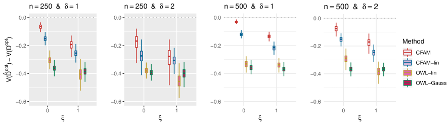
Figure 1: Boxplots obtained from $200$ Monte Carlo simulations comparing $4$ approaches to estimating $\mathcal{D}^{opt}$, given each scenario indexed by $\xi\in\{0,1\}$, $\delta\in\{1,2\}$ and $n\in\{250,500\}$. The dotted horizontal line represents the optimal value corresponding to $\mathcal{D}^{opt}$.

In Figure S.1, we present boxplots, obtained from $200$ simulation runs, of the normalized values $V(\widehat{\mathcal{D}}^{opt})$ (normalized by the optimal values $V(\mathcal{D}^{opt})$) of the decision rules $\widehat{\mathcal{D}}^{opt}$ estimated from the four approaches, for each combination of $n\in\{250,500\}$, $\xi\in\{0,1\}$ (corresponding to correctly-specified or mis-specified CFAM interaction models, respectively) and $\delta\in\{1,2\}$ (corresponding to moderate or large main effects, respectively). The results in Figure S.1 indicate that the proposed method (CFAM) outperforms all other approaches. In particular, if the sample size is relatively large $(n=500)$, for a correctly-specified CFAM ($\xi=0$) interaction underlying model, the proposed method gives a close-to-optimal performance in comparison to $\mathcal{D}^{opt}$. With nonlinearities present in the underlying model (S.13), CFAM-lin, which assumes a stringent linear structure on the interaction effect term, is outperformed by CFAM that utilizes the flexible component functions $g_{j}(\cdot,a)$ and $h_{k}(\cdot,a)$, while substantially outperforming the OWL-based approaches.

In Section A.5 of Supporting Information, we have also considered a similar set of experiments under a “linear” $A$-by-$\bm{X}$ interaction effect, in which CFAM-lin outperforms CFAM, but by a relatively small amount, whereas if the underlying model deviates from the exact linear structure and $n=500$, CFAM tends to outperform CFAM-lin. This suggests that, in the absence of prior knowledge about the form of the interaction effect, the more flexible CFAM that accommodates nonlinear treatment effect-modifications can be set as a default approach over CFAM-lin for optimizing ITRs. The estimated values of the OWL methods using linear and Gaussian kernels, respectively, are similar to each other, but both are outperformed by CFAM, even when CFAM is incorrectly specified (i.e., when $\xi=1$), as the current OWL methods do not directly deal with the functional pretreatment covariates. When the $(\bm{X},\bm{Z})$ “main” effect dominates the $A$-by-$(\bm{X},\bm{Z})$ interaction effect (i.e., when $\delta=2$), although the increased magnitude of this nuisance effect dampens the performance of all approaches to estimating $\mathcal{D}^{opt}$, the proposed approach outperforms all other methods.

In Table 1, we additionally illustrate the estimation performance for model parameters $\beta_{1}$ and $\beta_{2}$ when $\xi=0$ (i.e., when CFAM is correctly specified) with varying $\delta\in\{1,2\}$ and $n\in\{250,500,1000\}$, based on the root squared error $\mbox{RSE}(\beta_{j})=\sqrt{\int(\widehat{\beta}_{j}(s)-\beta_{j}(s))^{2}ds}$ $(j=1,2)$. In Figure 2, we display typical CFAM estimates $\widehat{\beta}_{j}$ of $\beta_{j}$ from 10 random samples, for each sample size $n$ (for the case of $\delta=1$). With sample size increasing, the estimators $\widehat{\beta}_{j}$ get close to the true coefficient functions $\beta_{j}$.

Table 1: The root squared error (RSE) of the estimates $\widehat{\beta}_{j}$ for $\beta_{j}$ $(j=1,2)$ for varying sample size $n\in\{250,500,1000\}$, when the “main” effect of $(\bm{X},\bm{Z})$ is moderate $(\delta=1)$ and large $(\delta=2)$, respectively.

	$\delta=1$ (Moderate “main” effect)			$\delta=2$ (Large “main” effect)
n	$250$	$500$	$1000$	$250$	$500$	$1000$
$\mbox{RSE}(\beta_{1})$	0.53(0.08)	0.34(0.02)	0.26(0.02)	0.60(0.14)	0.38(0.05)	0.29(0.03)
$\mbox{RSE}(\beta_{2})$	0.53(0.06)	0.34(0.02)	0.27(0.01)	0.59(0.13)	0.39(0.07)	0.29(0.03)

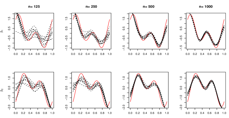
Figure 2: An illustration of typical $10$ CFAM sample estimates $\widehat{\beta}_{j}(s)$ (black dashed curves) for the parameters $\beta_{j}(s)$ (the red solid curves), for $j=1$ and $2$ in the top and bottom panels, respectively, with a varying training sample size $n\in\{125,250,500,1000\}$ for the case of $\delta=1$.

4.2 Treatment effect-modifier variable selection performance

In this subsection, we will report simulation results for the treatment effect-modifier selection among $\{X_{j},j=1,\ldots,p\}\cup\{Z_{k},k=1,\ldots,q\}$. The complexity of the $(\bm{X},\bm{Z})$-by-$A$ interaction terms of CFAM (S.1) can be summarized in terms of the size (cardinality) of the index set of $\{g_{j},j=1,\ldots,p\}\cup\{h_{k},k=1,\ldots,q\}$ that are not identically zero, each of which can be either correctly or incorrectly estimated to be equal to zero. As in Section 4.1, we generate $200$ datasets based on (S.13), with varying $\xi\in\{0,1\}$, $\delta\in\{1,2\}$ and sample size $n\in\{50,100,200,\ldots,700,800\}$ and $p=q=20$, i.e., we consider a total of $p+q=40$ potential treatment effect-modifiers, among which there are only $4$ “true” treatment effect-modifiers.

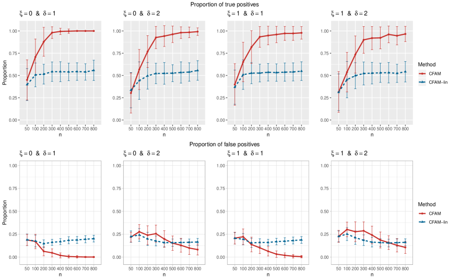
Figure 3: The proportion of the relevant covariates (i.e., the treatment effect-modifiers) correctly selected (the “true positives”; the top gray panels), and the “noise” covariates incorrectly selected (the “false positives”; the bottom white panels), respectively (and $\pm 1$ standard deviation), with a varying sample size $n\in\{50,100,200,\ldots,800\}$, for each combination of $\xi\in\{0,1\}$ and $\delta\in\{1,2\}$.

Figure 3 summarizes the results of the treatment effect-modifier covariate selection performance with respect to the true/false positive rates (the top/bottom panels, respectively), comparing the proposed CFAM and the CFAM-lin of Ciarleglio et al. (2018). The results are reported as the averages (and $\pm 1$ standard deviations) across the $200$ simulated datasets, for each simulation scenario. Figure 3 illustrates that the proportion of correct selection out of the $4$ true treatment effect-modifiers (i.e., the “true positive” rate; the top gray panels) of CFAM (the red solid curves) tends to $1$, as $n$ increases from $n=50$ to $n=800$, whereas the proportion of incorrect selection (i.e., the “false positive” rate; the bottom white panels) out of the $36$ irrelevant “noise” covariates tends to $0$; these proportions tend to either $1$ or $0$ quickly for moderate main effect ($\delta=1$) scenarios compared to large main effect ($\delta=2$) scenarios. On the other hand, the proportion of correct selections for CFAM-lin (the blue dotted curves), even with a large $n$, tends to be only around $0.55$, due to the stringent linear model assumption on the from of the $(\bm{X},\bm{Z})$-by-$A$ interaction effect.

5 Application

In this section, we illustrate the utility of CFAM for optimizing ITRs, using data from an RCT (Trivedi et al., 2016) comparing an antidepressant and placebo for treating major depressive disorder. The study collected various scalar and functional patient characteristics at baseline, including electroencephalogram (EEG) data. Study participants were randomized to either placebo ($A=1$) or an antidepressant (sertraline) ($A=2$). Subjects were monitored for 8 weeks after initiation of treatment. The primary endpoint of interest was the Hamilton Rating Scale for Depression (HRSD) score at week 8. The outcome $Y$ was taken to be the improvement in symptoms severity from baseline to week $8$ taken as the difference: week 0 HRSD score - week 8 HRSD score (larger values of the outcome $Y$ are considered desirable).

There were $n=180$ subjects. We considered $p=19$ pretreatment functional covariates consisting of the current source density (CSD) amplitude spectrum curves over the Alpha frequency range (observed while the participants’ eyes were open), measured from a subset of EEG channels from a total of 72 EEG electrodes which gives a fairly good spatial coverage of the scalp. The locations for these $19$ electrodes are indicated in the top panel of Figure 4. The Alpha frequency band ($8$ to $12$ Hz) considered as a potential biomarker of antidepressant response (e.g., Wade and Iosifescu, 2016) was scaled to $[0,1]$, hence each of the functional covariates $X=(X_{1}(s),\ldots,X_{19}(s))$ was defined on the interval $[0,1]$. We also considered $q=5$ baseline scalar covariates consisting of the week 0 HRSD score ($Z_{1}$), sex ($Z_{2}$), age at evaluation ($Z_{3}$), word fluency ($Z_{4}$) and Flanker accuracy ($Z_{5}$) cognitive test scores, which were identified as predictors of differential treatment response in a previous study (Park et al., 2020c). In this dataset, 49% of the subjects were randomized to the sertraline $(A=2)$. The average outcomes $Y$ for the sertraline and placebo groups were 7.41 and 6.29, respectively. The means (and standard deviations) of $Z_{1}$, $Z_{3}$, $Z_{4}$ and $Z_{5}$ were 18.59 (4.44), 37.7 (13.57), 38 (11.42) and 0.19 (0.11), respectively, and 67% of the subjects were female.

The proposed CFAM approach (4) selected two functional covariates: “C3” ($X_{4}$) and “P3” ($X_{5}$) (the selected electrodes are indicated by the red dashed circles in the top panel of Figure 4), and a scalar covariate: “Flanker accuracy test” ($Z_{5}$). In the first column of Figure 4, we display CSD curves corresponding to the selected two functional covariates, $X_{4}(s)$ and $X_{5}(s)$, from the $180$ subjects. In the second column of Figure 4, we display the estimated coefficient functions, $\widehat{\beta}_{4}(s)$ and $\widehat{\beta}_{5}(s)$ (with $95\%$ confidence bands conditional on the $j$th partial residual and the $j$th component function $\widehat{g}_{j}$), associated with those selected covariates.

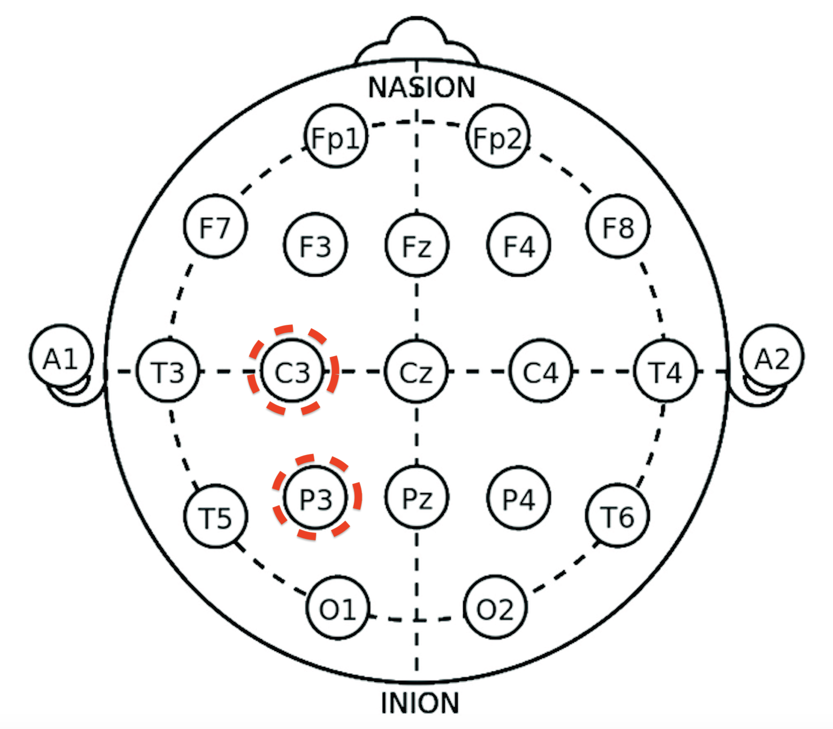
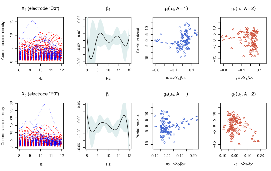
Figure 4: Top: The locations for the $19$ electrode channels (“A1” and “A2” were not used). Those marked in red circles are the selected electrodes from the proposed approach: “C3” and “P3”. Bottom: First column: observed current source density (CSD) curves from the selected channels $X_{4}$ (“C3”) and $X_{5}$ (“P3”), over the Alpha band ($8$ to $12$ Hz). Second column: the estimated single-index coefficient functions ($\beta_{4}$ and $\beta_{5}$) for the selected channels $X_{4}$ and $X_{5}$ (and the associated $95\%$ confidence bands, conditioning on the $j$th partial residual and the $j$th component function $\widehat{g}_{j}$). Third and fourth columns: the scatter plots of the ($j$th; $j=4,5$, top and bottom, respectively) partial residuals vs. the estimated single-indices $u_{4}=\langle X_{4},\beta_{4}\rangle$ and $u_{5}=\langle X_{5},\beta_{5}\rangle$, respectively, for the placebo $A=1$ (third column, blue circles) and sertraline $A=2$ (fourth column, red triangles) treated individuals, with the estimated treatment-specific component functions $g_{j}(u_{j},A)$ $(A=1,2)$ $(j=4,5)$ (the dashed curves) overlaid.

The coefficient functions $\widehat{\beta}_{j}(s)$ summarizing the $X_{j}(s)$ lead to data-driven indices $u_{j}=\langle\widehat{\beta}_{j},X_{j}\rangle\in\mathbb{R}$ that are linked to differential treatment response by two estimated nonzero component functions, $\widehat{g}_{j}(u_{j},A)$ $(j=4,5)$ in this example. In Figure 4, the fitted component functions, $\widehat{g}_{j}(u_{j},A)$ associated with the placebo $A=1$ (in the third column) and the active drug $A=2$ (in the fourth column), are displayed, along with the corresponding partial residuals. Roughly put, in Figure 4, the placebo $(A=1)$ effect tends to increase with the index $u_{j}$ $(j=4,5)$ whereas the sertraline $(A=2)$ effect decreases with the index. In the second column of Figure 4, both $\beta_{4}$ and $\beta_{5}$ put a bulk of their negative weight on lower frequencies (8 to 9 Hz), meaning that patients whose CSD values are small in those frequency regions would have large values of $\langle\beta_{j},X_{j}\rangle$, over the values which the placebo effects are predicted to be relatively strong, in comparison to the sertraline effects.

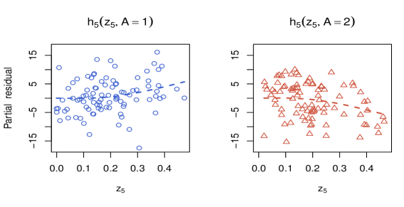
Figure 5: The scatter plots of the $k$th partial residual vs. the $k$th scalar covariate, for the selected $5$th scalar covariate $Z_{5}$ “Flanker accuracy test score,” for the placebo $A=1$ (first column, blue circles) and sertraline $A=2$ (second column, red triangles) treated individuals, with the estimated treatment-specific component functions $h_{5}(z_{5},A)$ $(A=1,2)$ (the dashed curves) overlaid.

To evaluate the performance of ITRs $(\widehat{\mathcal{D}}^{opt})$ estimated from the four different approaches described in Section 4, we randomly split the data into a training set and a testing set (of size $\widetilde{n}$) using a ratio of $5:1$, replicated $500$ times, each time estimating an ITR $\widehat{\mathcal{D}}^{opt}$ based on the training set, and its “value” $V(\widehat{\mathcal{D}}^{opt})=E[E[Y|\bm{X},\bm{Z},A=\widehat{\mathcal{D}}^{opt}(\bm{X},\bm{Z})]]$, by an inverse probability weighted estimator (Murphy, 2005) $\widehat{V}(\widehat{\mathcal{D}}^{opt})=\sum_{i=1}^{\widetilde{n}}Y_{i}I_{(A_{i}=\widehat{\mathcal{D}}^{opt}(\bm{X}_{i},\bm{Z}_{i}))}/\sum_{i=1}^{\widetilde{n}}I_{(A_{i}=\widehat{\mathcal{D}}^{opt}(\bm{X}_{i},\bm{Z}_{i}))}$, computed based on the testing set (of size $\widetilde{n}$). For comparison, we also include two naïve rules: treating all patients with placebo (“All PBO”) and treating all patients with the active drug (“All DRUG”), each regardless of the individual patient’s characteristics $(\bm{X},\bm{Z})$. The resulting boxplots obtained from the $500$ random splits are illustrated in Figure 6.

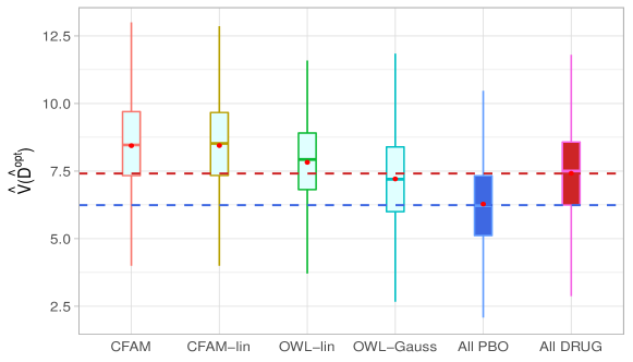
Figure 6: Boxplots of the estimated values of the treatment rules $\widehat{\mathcal{D}}^{opt}$ estimated from $6$ approaches, obtained from $500$ randomly split testing sets. Higher values are preferred.

The results in Figure 6 demostrate that CFAM and CFAM-lin perform at a similar level, showing a clear advantage over the both OWL-lin and OWL-Gauss, suggesting that regression utilizing the functional nature of the EEG measurements, that targets the treatment-by-functional covariates interactions is well-suited in this example. Specifically, in Figure 6, the superiority of CFAM (or CFAM-lin) over the policy of treating everyone with the drug (All DRUG) was of similar magnitude of the superiority of All DRUG over All PBOs. This suggests that accounting for patient characteristics can help treatment decisions. In this example, as can be observed from the third and fourth columns of Figures 4 and 5, the estimated nonlinear treatment effect-modification is rather modest. As a result, the performances of CFAM and CFAM-lin are comparable to each other. However, as demonstrated in Section 4, the more flexible CFAM can be employed as a default approach over CFAM-lin, allowing for potentially essential nonlinearities in treatment effect-modification.

6 Discussion

We have developed a functional additive regression approach specifically focused on extracting possibly nonlinear pertinent interaction effects between treatment and multiple functional/scalar covariates, which is of paramount importance in developing effective ITRs for precision medicine. This is accomplished by imposing appropriate structural constraints, performing treatment effect-modifier selection and extracting one-dimensional functional indices. The estimation approach utilizes an efficient coordinate-descent for the component functions and a functional linear model estimation procedure for the coefficient functions. The proposed functional regression for ITRs extends existing methods by incorporating possibly nonlinear treatment-by-functional covariates interactions. Encouraged by our simulation results and the application, future work will investigate the asymptotic properties of the method related to variable selection and estimation consistency, and a hypothesis testing framework for significant interactions between treatment and functional covariates.

SUPPLEMENTARY MATERIAL

Supplementary Material at the end of the document provides additional technical details referred to in the main paper, including the proof of Theorem 1. Supplementary Material also presents additional simulation examples, including a set of simulation experiments with a “linear” $A$-by-$(\bm{X},\bm{Z})$ interaction effect scenario.

R-package:

R-package famTEMsel (Functional Additive Models for Treatment Effect-Modifier Selection) contains R-codes to perform the methods proposed in the article, and is publicly available on GitHub (syhyunpark/famTEMsel).

Conflict of interest

None declared.

SUPPLEMENTARY MATERIAL

Appendix A: Technical details and additional simulations

A.1. Description of the constrained least squares criterion in Section 2.1

In Section 2 of the main manuscript, we introduce the constrained functional additive model (CFAM) for the $(\bm{X},\bm{Z})$-by-$A$ interaction effect:

$$Y\ =\mu(\bm{X},\bm{Z})+\sum_{j=1}^{p}g_{j}(\langle X_{j},\beta_{j}\rangle,A)+\sum_{k=1}^{q}h_{k}(Z_{k},A)\ +\ \epsilon,$$ (S.1)

with $\beta_{j}\in\Theta$, subject to the constraint on the component functions $g_{j}\in\mathcal{H}_{j}^{(\beta_{j})}$ $(j=1,\ldots,p)$ and $h_{k}\in\mathcal{H}_{k}$ $(k=1,\ldots,q)$:

$$E[g_{j}(\langle X_{j},\beta_{j}\rangle,A)|X_{j}] =0\quad\mbox{(almost surely)}\quad(\forall\beta_{j}\in\Theta)\quad(j=1,\ldots,p)\quad\mbox{and}$$ (S.2)

$$E[h_{k}(Z_{k},A)|Z_{k}] =0\quad\mbox{(almost surely)}\quad(k=1,\ldots,q),$$

in which the expectation is taken with respect to the distribution of $A$ given $X_{j}$ (or $Z_{k}$), and $\epsilon\in\mathbb{R}$ is a mean zero noise with finite variance, and the form of the squared integrable functional $\mu$ in (S.1) is left unspecified.

Under model (S.1) subject to (S.2), the “true” (i.e., optimal) functional components, which we denote by $\{g_{j}^{\ast},j=1,\ldots,p\}\cup\{\beta_{j}^{\ast},j=1,\ldots,p\}\cup\{h_{k}^{\ast},k=1,\ldots,q\}$ that constitute the $(\bm{X},\bm{Z})$-by-$A$ interaction effect, can be specified and viewed as the solution to the following constrained least squares problem:

$$\{g_{j}^{\ast},\beta_{j}^{\ast},h_{k}^{\ast}\}\quad= \underset{g_{j}\in\mathcal{H}_{j}^{(\beta_{j})},\beta_{j}\in\Theta,h_{k}\in\mathcal{H}_{k}}{\text{argmin}} E\bigg{[}\bigg{\{}Y-\mu(\bm{X},\bm{Z})-\sum_{j=1}^{p}g_{j,A}(\langle X_{j},\beta_{j}\rangle)-\sum_{k=1}^{q}h_{k,A}(Z_{k})\bigg{\}}^{2}\bigg{]}$$ (S.3)

subject to $$E[g_{j,A}(\langle X_{j},\beta_{j}\rangle)|X_{j}]=0\quad\forall\beta_{j}\in\Theta\quad(j=1,\ldots,p)\quad\mbox{and}$$

$$E[h_{k,A}(Z_{k})|Z_{k}]=0\quad(k=1,\ldots,q),$$

in which $\mu(\bm{X},\bm{Z})$ is the “main” effect component appeared in model (S.1) (and is considered as fixed in (S.3)). In particular, on the right-hand side of (S.3), the expected squared error criterion term can be expanded as:

$$\operatorname*{arg\,min}_{g_{j}\in\mathcal{H}_{j}^{(\beta_{j})},\beta_{j}\in\Theta,h_{k}\in\mathcal{H}_{k}}\mathbb{E}\bigg{[}\bigg{\{}Y-\sum_{j=1}^{p}g_{j,A}(\langle X_{j},\beta_{j}\rangle)-\sum_{k=1}^{q}h_{k,A}(Z_{k})\bigg{\}}^{2}+2\mu(\bm{X},\bm{Z})\bigg{\{}\sum_{j=1}^{p}g_{j,A}(\langle X_{j},\beta_{j}\rangle)+\sum_{k=1}^{q}h_{k,A}(Z_{k})\bigg{\}}\bigg{]}$$

$$= \operatorname*{arg\,min}_{g_{j}\in\mathcal{H}_{j}^{(\beta_{j})},\beta_{j}\in\Theta,h_{k}\in\mathcal{H}_{k}}\mathbb{E}\left[\bigg{\{}Y-\sum_{j=1}^{p}g_{j,A}(\langle X_{j},\beta_{j}\rangle)-\sum_{k=1}^{q}h_{k,A}(Z_{k})\bigg{\}}^{2}+2\mu(\bm{X},\bm{Z})\mathbb{E}\bigg{[}\sum_{j=1}^{p}g_{j,A}(\langle X_{j},\beta_{j}\rangle)+\sum_{k=1}^{q}h_{k,A}(Z_{k})|\bm{X},\bm{Z}\bigg{]}\right]$$

$$= \operatorname*{arg\,min}_{g_{j}\in\mathcal{H}_{j}^{(\beta_{j})},\beta_{j}\in\Theta,h_{k}\in\mathcal{H}_{k}}\mathbb{E}\bigg{[}\bigg{\{}Y-\sum_{j=1}^{p}g_{j,A}(\langle X_{j},\beta_{j}\rangle)-\sum_{k=1}^{q}h_{k,A}(Z_{k})\bigg{\}}^{2}\bigg{]},$$

in which the second line follows from an application of the iterated expectation rule to condition on $(\bm{X},\bm{Z})$ on the second term on the first line, and the third line follows from the constraint imposed in (S.3), that is, $\mathbb{E}[g_{j,A}(\langle X_{j},\beta_{j}\rangle)|X_{j}]=0,\ \forall\beta_{j}\in\Theta\ (j=1,\ldots,p)$ and $\mathbb{E}[h_{k,A}(Z_{k})|Z_{k}]=0$  $(k=1,\ldots,q)$, which makes the second term on the second line of the above expression vanish to zero.

Since the minimization in (S.3) is in terms of $\{g_{j},\beta_{j},h_{k}\}$, the right-hand side of (S.3) can then be reduced to:

$$\{g_{j}^{\ast},\beta_{j}^{\ast},h_{k}^{\ast}\}\quad= \underset{g_{j}\in\mathcal{H}_{j}^{(\beta_{j})},\beta_{j}\in\Theta,h_{k}\in\mathcal{H}_{k}}{\text{argmin}} E\bigg{[}\bigg{\{}Y-\sum_{j=1}^{p}g_{j}(\langle X_{j},\beta_{j}\rangle,A)-\sum_{k=1}^{q}h_{k}(Z_{k},A)\bigg{\}}^{2}\bigg{]}$$ (S.4)

subject to $$E\left[g_{j}(\langle X_{j},\beta_{j}\rangle,A)|X_{j}\right]=0\quad\forall\beta_{j}\in\Theta\quad(j=1,\ldots,p)\quad\mbox{and}$$

$$E\left[h_{k}(Z_{k},A)|Z_{k}\right]=0\quad(k=1,\ldots,q),$$

which is as appeared in the representation (3) of the main manuscript.

A.2. Proof of Theorem 1

In this subsection, we provide the proof of Theorem 1 in Section 3.1 of the main manuscript. In order to simplify the exposition, we focus on the derivation of the minimizing functions $g_{j}\in\mathcal{H}_{j}^{(\beta_{j})}$ $(j=1,\ldots,p)$ associated with the functional covariates $X_{j}$ $(j=1,\ldots,p)$, only. The minimizing functions $h_{k}\in\mathcal{H}_{k}$ $(k=1,\ldots,q)$ associated with the scalar covariates $Z_{k}$ $(k=1,\ldots,q)$ are derived in the similar way. Further, for fixed $\beta_{j}\in\Theta$ $(j=1,\ldots,p)$, we write $X_{\beta_{j}}=\langle X_{j},\beta_{j}\rangle\in\mathbb{R}$ $(j=1,\ldots,p)$, for notational simplicity.

The squared error criterion on the right-hand side of (S.4) is

$$\mathbb{E}\bigg{[}\big{\{}Y-\sum_{j=1}^{p}g_{j}(X_{\beta_{j}},A)\big{\}}^{2}\bigg{]}\propto \ \mathbb{E}\bigg{[}Y\sum_{j=1}^{p}g_{j}(X_{\beta_{j}},A)-\big{\{}\sum_{j=1}^{p}g_{j}(X_{\beta_{j}},A)\big{\}}^{2}/2\bigg{]}\quad\mbox{(with respect to }\{g_{j}\})$$ (S.5)

$$= \ \mathbb{E}\bigg{[}\big{\{}\mu(\bm{X})+\sum_{j=1}^{p}g_{j}^{\ast}(X_{\beta_{j}^{\ast}},A)\big{\}}\sum_{j=1}^{p}g_{j}(X_{\beta_{j}},A)-\big{\{}\sum_{j=1}^{p}g_{j}(X_{\beta_{j}},A)\big{\}}^{2}/2\bigg{]}$$

$$= \ \mathbb{E}\bigg{[}\mu(\bm{X})\sum_{j=1}^{p}g_{j}(X_{\beta_{j}},A)\bigg{]}+\mathbb{E}\bigg{[}\big{\{}\sum_{j=1}^{p}g_{j}^{\ast}(X_{\beta_{j}^{\ast}},A)\big{\}}\big{\{}\sum_{j=1}^{p}g_{j}(X_{\beta_{j}},A)\big{\}}-\big{\{}\sum_{j=1}^{p}g_{j}(X_{\beta_{j}},A)\big{\}}^{2}/2\bigg{]}$$

$$= \ \mathbb{E}\bigg{[}\big{\{}\sum_{j=1}^{p}g_{j}^{\ast}(X_{\beta_{j}^{\ast}},A)\big{\}}\big{\{}\sum_{j=1}^{p}g_{j}(X_{\beta_{j}},A)\big{\}}-\big{\{}\sum_{j=1}^{p}g_{j}(X_{\beta_{j}},A)\big{\}}^{2}/2\bigg{]},$$

where the last equality follows from the constraint $\mathbb{E}[g_{j}(X_{\beta_{j}},A)|X_{j}]=0$ $(j=1,\ldots,p)$ in (S.4) imposed on $\{g_{j}\}$, which implies $\mathbb{E}\big{[}\mu(\bm{X})\big{\{}\sum_{j=1}^{p}g_{j}\big{(}X_{\beta_{j}},A\big{)}\big{\}}\big{]}=\mathbb{E}\big{[}\mathbb{E}\big{[}\mu(\bm{X})\big{\{}\sum_{j=1}^{p}g_{j}(X_{\beta_{j}},A)\big{\}}\mid\bm{X}\big{]}\big{]}=\mathbb{E}\big{[}\mu(\bm{X})\sum_{j=1}^{p}\mathbb{E}\big{[}g_{j}(X_{\beta_{j}},A)\mid X_{j}\big{]}\big{]}=0$. From (S.5), for fixed $\{\beta_{j},j=1,\ldots,p\}$, we can rewrite the squared error criterion in (S.4) by (omitting the components associated with the scalar covariates):

$$\underset{\{g_{j}\in\mathcal{H}_{j}^{(\beta_{j})}\}}{\text{argmin}}\ \mathbb{E}\bigg{[}\big{(}Y-\sum_{j=1}^{p}g_{j}\big{(}X_{\beta_{j}},A\big{)}\big{)}^{2}\bigg{]}\ =\ \underset{\{g_{j}\in\mathcal{H}_{j}^{(\beta_{j})}\}}{\text{argmin}}\ \mathbb{E}\bigg{[}\big{(}\sum_{j=1}^{p}g_{j}^{\ast}\big{(}X_{\beta_{j}^{\ast}},A\big{)}-\sum_{j=1}^{p}g_{j}\big{(}X_{\beta_{j}},A\big{)}\big{)}^{2}\bigg{]}.$$ (S.6)

In the following, we closely follow the proof of Theorem 1 in Ravikumar et al. (2009). The Lagrangian in (4) of the main manuscript, for fixed $\{\beta_{j},j=1,\ldots,p\}$ can be rewritten as:

$$Q(\{g_{j}\};\lambda):=\mathbb{E}\bigg{[}\big{(}\sum_{j=1}^{p}g_{j}^{\ast}(X_{\beta_{j}^{\ast}},A)-\sum_{j=1}^{p}g_{j}(X_{\beta_{j}},A)\big{)}^{2}\bigg{]}+\lambda\sum_{j=1}^{p}\lVert g_{j}\rVert.$$ (S.7)

Fixing $\{\beta_{j},j=1,\ldots,p\}$, for each $j$, let us consider the minimization of (S.7) with respect to the component function $g_{j}\in\mathcal{H}_{j}^{(\beta_{j})}$, holding the other component functions $\{g_{j^{\prime}},j^{\prime}\neq j\}$ fixed. The stationary condition is obtained by setting its Fréchet derivative to 0. Denote by $\partial_{j}Q(\{g_{j}\};\lambda;\eta_{j})$ the directional derivative with respect to $g_{j}\in\mathcal{H}_{j}^{(\beta_{j})}$ $(j=1,\ldots,p)$ in an arbitrary direction which we denote by $\eta_{j}\in\mathcal{H}_{j}^{(\beta_{j})}$. Then, for fixed $\{\beta_{j},j=1,\ldots,p\}$, the stationary point of the Lagrangian (S.7) can be formulated as:

$$\partial_{j}Q(\{g_{j}\};\lambda;\eta_{j})=2\mathbb{E}\left[(g_{j}-\widetilde{R}_{j}+\lambda\nu_{j})\eta_{j}\right]=0,$$ (S.8)

where

$$\widetilde{R}_{j}:=\sum_{j=1}^{p}g_{j}^{\ast}(X_{\beta_{j}^{\ast}},A)-\sum_{j^{\prime}\neq j}g_{j^{\prime},A}(X_{\beta_{j^{\prime}}}),$$ (S.9)

representing the partial residual for the $j$th component function $g_{j}$, and the function $\nu_{j}$ is an element of the subgradient $\partial\lVert g_{j}\rVert$, which satisfies $\nu_{j}=g_{j}/\lVert g_{j}\rVert$ if $\lVert g_{j}\rVert\neq 0$, and $\nu_{j}\in\{s\in\mathcal{H}_{j}^{(\beta_{j})}\mid\lVert s\rVert\leq 1\}$, otherwise. Applying the iterated expectations to condition on $(X_{\beta_{j}},A)$, the stationary condition (S.8) can be rewritten as:

$$2\mathbb{E}\left[\left(g_{j}-\mathbb{E}\left[\widetilde{R}_{j}|X_{\beta_{j}},A\right]+\lambda\nu_{j}\right)\eta_{j}\right]=0.$$ (S.10)

Since the function $g_{j}-\mathbb{E}\left[\widetilde{R}_{j}|X_{\beta_{j}},A\right]+\lambda\nu_{j}\in\mathcal{H}_{j}^{(\beta_{j})}$, we can evaluate (S.8) (i.e., expression (S.10)) in the particular direction: $\eta_{j}=g_{j}-\mathbb{E}\left[\widetilde{R}_{j}|X_{\beta_{j}},A\right]+\lambda\nu_{j}$, which gives $\mathbb{E}\left[\left(g_{j}-\mathbb{E}\left[\widetilde{R}_{j}|X_{\beta_{j}},A\right]+\lambda\nu_{j}\right)^{2}\right]=0.$ This equation implies:

$$g_{j}+\lambda\nu_{j}=\mathbb{E}\left[\widetilde{R}_{j}|X_{\beta_{j}},A\right]\quad\mbox{(almost surely).}$$ (S.11)

Let $f_{j}$ denote the right-hand side of (S.11), i.e., $f_{j}(=f_{j}(X_{\beta_{j}},A)):=\mathbb{E}\left[\widetilde{R}_{j}|X_{\beta_{j}},A\right]$. If $\lVert g_{j}\rVert\neq 0$, then $\nu_{j}=g_{j}/\lVert g_{j}\rVert$. Therefore, by (S.11), we have $\lVert f_{j}\rVert=\lVert g_{j}+\lambda g_{j}/\lVert g_{j}\rVert\rVert=\lVert g_{j}\rVert+\lambda\geq\lambda$. On the other hand, if $\lVert g_{j}\rVert=0$, then $g_{j}=0$ (almost surely), and $\lVert\nu_{j}\rVert\leq 1$. Then, condition (S.11) implies that $\lVert f_{j}\rVert\leq\lambda$. This gives us the equivalence between $\lVert f_{j}\rVert\leq\lambda$ and the statement $g_{j}=0$ (almost surely). Therefore, condition (S.11) leads to the following expression:

$$\left(1+\lambda/\lVert g_{j}\rVert\right)g_{j}=f_{j}\quad\mbox{(almost surely)}$$

if $\lVert f_{j}\rVert>\lambda$, and $g_{j}=0$ (almost surely), otherwise; this implies the soft thresholding update rule for $g_{j}$ appeared in (5) of the main manuscript.

Now we will derive the expression (6) of the main manuscript for the function $f_{j}$. Note, the underlying model (S.1) (if we omit the components associated with the scalar covariates) implies that $\sum_{j=1}^{p}g_{j}^{\ast}(X_{\beta_{j}^{\ast}},A)=\mathbb{E}[Y|\bm{X},A]-\mu(\bm{X})$. Thus, (S.9) can be equivalently written as: $\widetilde{R}_{j}=\mathbb{E}[Y|\bm{X},A]-\mu(\bm{X})-\sum_{j^{\prime}\neq j}g_{j^{\prime}}(X_{\beta_{j^{\prime}}},A).$ Therefore, the function $f_{j}(X_{\beta_{j}},A)=\mathbb{E}\left[\widetilde{R}_{j}|X_{\beta_{j}},A\right]$ can be written as:

$$f_{j}(X_{\beta_{j}},A) =\mathbb{E}\big{[}\mathbb{E}[Y|\bm{X},A]-\mu(\bm{X})-\sum_{j^{\prime}\neq j}g_{j^{\prime}}(X_{\beta_{j^{\prime}}},A)\mid X_{\beta_{j}},A\big{]}$$

$$=\mathbb{E}\big{[}\mathbb{E}[Y|\bm{X},A]-\sum_{j^{\prime}\neq j}g_{j^{\prime}}(X_{j^{\prime}},A)\mid X_{\beta_{j}},A\big{]}-\mathbb{E}\big{[}\mu(\bm{X})\mid X_{\beta_{j}},A\big{]}$$

$$=\mathbb{E}\big{[}Y-\sum_{j^{\prime}\neq j}g_{j^{\prime}}(X_{\beta_{j^{\prime}}},A)\mid X_{\beta_{j}},A\big{]}-\mathbb{E}\big{[}\mu(\bm{X})\mid X_{\beta_{j}}\big{]}$$

$$=\mathbb{E}\big{[}Y-\sum_{j^{\prime}\neq j}g_{j^{\prime}}(X_{\beta_{j^{\prime}}},A)\mid X_{\beta_{j}},A\big{]}-\mathbb{E}\big{[}\mu(\bm{X})+\sum_{j=1}^{p}g_{j}^{\ast}\big{(}X_{\beta_{j}^{\ast}},A\big{)}\mid X_{\beta_{j}}\big{]}$$

$$=\mathbb{E}\big{[}Y-\sum_{j^{\prime}\neq j}g_{j^{\prime}}(X_{\beta_{j^{\prime}}},A)\mid X_{\beta_{j}},A\big{]}-\mathbb{E}\big{[}Y\mid X_{\beta_{j}}\big{]}$$

$$=\mathbb{E}\big{[}Y-\sum_{j^{\prime}\neq j}g_{j^{\prime}}(X_{\beta_{j^{\prime}}},A)\mid X_{\beta_{j}},A\big{]}-\mathbb{E}\big{[}Y-\sum_{j^{\prime}\neq j}g_{j^{\prime}}(X_{\beta_{j^{\prime}}},A)\mid X_{\beta_{j}}\big{]}$$

$$=\mathbb{E}\big{[}R_{j}\mid X_{\beta_{j}},A\big{]}-\mathbb{E}\big{[}R_{j}\mid X_{\beta_{j}}\big{]},$$

where the fourth equality of the expression follows from the identifiability constraint (S.2) of the underlying model (S.1), and the sixth equality follows from the optimization constraint $\mathbb{E}[g_{j^{\prime}}(X_{\beta_{j^{\prime}}},A)|X_{j}]=0$ $(j^{\prime}\neq j)$ implied by (S.4) imposed on $\{g_{j^{\prime}},j^{\prime}\neq j\}$; this gives the expression (6) of the main manuscript for $f_{j}$.

A.3. Description of general linear smoothers for the component functions

As a remark to Section 3.2.1 of the main manuscript, we note that any scatterplot smoother can be utilized to obtain the sample counterpart (16) of the main manuscript of the coordinate-wise solution (5) for the component functions $g_{j}$, i.e., estimation of the component functions $g_{j}$ is not restricted to regression splines.

To estimate the function $f_{j}$ in (6), we can estimate the system of treatment $a$-specific functions $\mathbb{E}[R_{j}|\langle\widehat{\beta}_{j},X_{ij}\rangle,A=a]$ $(a=1,\ldots,L)$ (which corresponds to the first term on the right-hand side of (6) if we fix $\beta_{j}=\widehat{\beta}_{j}$), by performing separate nonparametric regressions of $\widehat{R}_{j}$ on regressor $\langle\widehat{\beta}_{j},X_{ij}\rangle$ separately for each treatment condition $A=a$ $(a=1,\ldots,L)$. We can also estimate the function $-\mathbb{E}[R_{j}|\langle\beta_{j},X_{ij}\rangle]$ (which corresponds to the second term $-\mathbb{E}[R_{j}|\langle\beta_{j},X_{ij}\rangle]$ on the right-hand side of (6) if we fix $\beta_{j}=\widehat{\beta}_{j}$), by performing a nonparametric regression of $\widehat{R}_{j}$ on regressor $\langle\widehat{\beta}_{j},X_{ij}\rangle$. Adding these two function estimates provides an estimate for $f_{j}$ in (6). Evaluating this estimate of $f_{j}$ at the $n$ points $(\langle\widehat{\beta}_{j},X_{ij}\rangle,A_{i})$ $(i=1,\ldots,n)$ gives an estimate $\widehat{\bm{f}}_{j}\in\mathbb{R}^{n}$ in (16). Then we can compute the corresponding soft-threshold estimate $\widehat{\bm{g}}_{j}\in\mathbb{R}^{n}$ and conduct the coordinate descent procedure described in Algorithm 1 of the main manuscript.

A.4. Supplementary information for Section 3.2.1

The restriction of the function $g_{j}$ to the form (12) of the main manuscript restricts also the minimizing function $g_{j}$ in (5) of the main manuscript (note, $g_{j}(\langle X_{j},\widehat{\beta}_{j}\rangle,A)=s_{j}^{(\lambda)}f_{j}(\langle X_{j},\widehat{\beta}_{j}\rangle,A)$, where $s_{j}^{(\lambda)}=\left[1-\lambda/\lVert f_{j}\rVert\right]_{+}$) to the form (12) of the main manuscript. In particular, we can express the function $f_{j}$ in (6) of the main manuscript as:

$$f_{j,A}(\langle X_{j},\widehat{\beta}_{j}\rangle) =\ \mathbb{E}[R_{j}|\langle X_{j},\widehat{\beta}_{j}\rangle,A]-\sum_{a=1}^{L}\pi_{a}\mathbb{E}[R_{j}|\langle X_{j},\widehat{\beta}_{j}\rangle,A=a]$$ (S.12)

$$=\ \bm{\Psi}_{j}(\langle X_{j},\widehat{\beta}_{j}\rangle)\bm{\theta}_{j,A}^{\ast}-\bm{\Psi}_{j}(\langle X_{j},\widehat{\beta}_{j}\rangle)\{\sum_{a=1}^{L}\pi_{a}\bm{\theta}_{j,a}^{\ast}\},$$

where $\{\bm{\theta}_{j,a}^{\ast}\}_{a\in\{1,\ldots,L\}}:=\underset{\{\bm{\theta}_{j,a}\in\mathbb{R}^{d_{j}}\}_{a\in\{1,\ldots,L\}}}{\text{argmin}}\mathbb{E}\left[\big{\{}R_{j}-\bm{\Psi}_{j}(\langle X_{j},\widehat{\beta}_{j}\rangle)^{\top}\bm{\theta}_{j,A}\big{\}}^{2}\right]$. In (S.12), the first term, $\bm{\Psi}_{j}(\langle X_{j},\widehat{\beta}_{j}\rangle)\bm{\theta}_{j,A}^{\ast}$, corresponds to the $L^{2}$ projection of the $j$th partial residual $R_{j}$ in (7) (of the main manuscript) onto the class of functions of the form (12) (without the imposition of the constraint (13), that is, the constraint $\sum_{a=1}^{L}\pi_{a}\bm{\theta}_{j,a}=\bm{0}$), whereas the second term, $-\bm{\Psi}_{j}(\langle X_{j},\widehat{\beta}_{j}\rangle)\{\sum_{a=1}^{L}\pi_{a}\bm{\theta}_{j,a}^{\ast}\}$, simply centers the first term to satisfy the linear constraint, $\sum_{a=1}^{L}\pi_{a}\bm{\theta}_{j,a}=\bm{0}$. Then it follows that $f_{j}$, as given in (S.12), corresponds to the $L^{2}$ projection of $R_{j}$ onto the subspace of measurable functions of the form (12) subject to the linear constraint (13) of the main manuscript.

A.5. Simulation results under a “linear” $A$-by-$(\bm{X},\bm{Z})$ interaction effect scenario

In this subsection, as an extension of the simulation example in Section 4.1 of the main manuscript, we consider a case where the treatment effect varies linearly in the covariates $(\bm{X},\bm{Z})$, i.e., a “linear” $A$-by-$(\bm{X},\bm{Z})$ interaction effect scenario and assess the ITR estimation performance of the methods. Specifically, we consider the data generation model:

$$Y_{i} =\delta\bigg{\{}\sum_{j=1}^{8}\sin(\langle\eta_{j},X_{ij}\rangle)+\sum_{k=1}^{8}\sin(Z_{ik})\bigg{\}}+$$ (S.13)

$$4(A_{i}-1.5)\bigg{[}\langle\beta_{1},X_{i1}\rangle/1.5-\langle\beta_{2},X_{i2}\rangle/1.5+Z_{i1}/1.5-Z_{i2}/1.5+\xi\big{\{}\langle X_{i1},X_{i2}\rangle/1.5+Z_{i1}Z_{i2}/1.5\big{\}}\bigg{]}+\epsilon_{i},$$

in which, when $\xi=0$, a functional linear model specifies the $A$-by-$(\bm{X},\bm{Z})$ interaction effect term (i.e., the second term on the right-hand side of (S.13)). However, when $\xi=1$, the underlying model (S.13) deviates from the exact linear $A$-by-$(\bm{X},\bm{Z})$ interaction effect structure, and in such a case, the model CFAM-lin (as well as CFAM) is misspecified. The contribution to the variance of $Y$ from the main and the interaction effect terms in (S.13) was made similar to that of the data generating model (25) of Section 4.1 of the main manuscript.

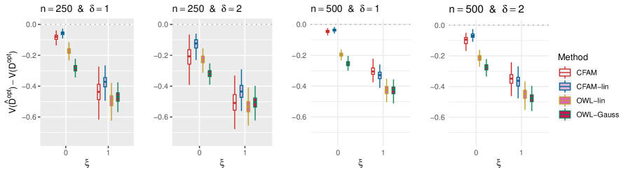
Figure S.1: Boxplots obtained from $200$ Monte Carlo simulations comparing $4$ approaches to estimating $\mathcal{D}^{opt}$, given each scenario indexed by $\xi\in\{0,1\}$, $\delta\in\{1,2\}$ and $n\in\{250,500\}$. The dotted horizontal line represents the optimal value corresponding to $\mathcal{D}^{opt}$.

Figure S.1 illustrates the boxplots, obtained from $200$ simulation runs, of the normalized values $V(\widehat{\mathcal{D}}^{opt})-V(\mathcal{D}^{opt})$ (normalized by the optimal values $V(\mathcal{D}^{opt})$) of the decision rules $\widehat{\mathcal{D}}^{opt}$ estimated from the four approaches described in Section 4.1 of the main manuscript, for each combination of $n\in\{250,500\}$, $\xi\in\{0,1\}$ (corresponding to correctly-specified or mis-specified CFAM scenarios, respectively) and $\delta\in\{1,2\}$ (corresponding to moderate or large main effects, respectively).

In all scenarios with $\xi=0$ (i.e., when the linear interaction model is correctly specified), CFAM-lin outperforms CFAM, but by a relatively small amount in comparison to the difference in performance appearing in Figure 1 of the main manuscript, in which CFAM outperforms CFAM-lin. Moreover, if the underlying model deviates from the exact linear structure (i.e., $\xi=1$ in model (S.13)) and $n=500$, the more flexible CFAM tends to outperform CFAM-lin. Given the outstanding performance of CFAM compared to CFAM-lin in the nonlinear $A$-by-$(\bm{X},\bm{Z})$ interaction effect scenarios considered in the main manuscript, this result suggests that, in the absence of prior knowledge about the form of the interaction effect, flexible modeling of the interaction effect using the proposed CFAM can lead to good results in comparison to CFAM-lin.

A.6. Separate modeling of the $(\bm{X},\bm{Z})$ “main” effect component

Under model (S.1), constraint (S.2) (i..e, constraint (2) of the main manuscript) ensures that

$$E\left[\mu(\bm{X},\bm{Z})\left\{\sum_{j=1}^{p}g_{j}(\langle X_{j},\beta_{j}\rangle,A)+\sum_{k=1}^{q}h_{k}(Z_{k},A)\right\}\right]=E\left[\mu(\bm{X},\bm{Z})E\left\{\sum_{j=1}^{p}g_{j}(\langle X_{j},\beta_{j}\rangle,A)+\sum_{k=1}^{q}h_{k}(Z_{k},A)\mid\bm{X},\bm{Z}\right\}\right]=0,$$

where, on the right-hand side, we apply the iterated expectation rule to condition on $(\bm{X},\bm{Z})$, which implies:

$$\mu(\bm{X},\bm{Z})\quad\perp\quad\sum_{j=1}^{p}g_{j}(\langle X_{j},\beta_{j}\rangle,A)+\sum_{k=1}^{q}h_{k}(Z_{k},A)$$ (S.14)

in $L^{2}$. The orthogonality (S.14) conceptually and also practically implies that, under the squared error minimization criterion, the optimization for $\mu$ and the components $\{g_{j},\beta_{j},h_{k}\}$ in model (S.1) (subject to (S.2)) can be performed separately, without iterating between the two optimization procedures. To be specific, we can solve for the $(\bm{X},\bm{Z})$ “main” effect:

$$\mu^{\ast}\quad=\quad\underset{\mu\in\mathcal{H}}{\text{argmin}}\quad E\left[\left\{Y-\mu(\bm{X},\bm{Z})\right\}^{2}\right],$$ (S.15)

and can separately solve for the $(\bm{X},\bm{Z})$-by-$A$ interaction effect via optimization (S.4). In optimization (S.15), $\mathcal{H}$ represents a (possibly misspecified) $L^{2}$ space of functionals over $(\bm{X},\bm{Z})$. Even if the true $\mu$ in (S.1) is not in the class $\mathcal{H}$, the representation (S.4) that specifies the optimal $(\bm{X},\bm{Z})$-by-$A$ interaction effect components, i.e., $\{g_{j}^{\ast},\beta_{j}^{\ast},h_{k}^{\ast}\}$, is not affected by the possible misspecification for $\mu$, due to the orthogonality (S.14).

For the case of a continuous outcome $Y$, Tian et al. (2014) (in the linear regression context with scalar covariates and Lasso regularization) and Park et al. (2020a) (in the single-index regression context with scalar covariates) proposed to separately model and fit the main effect component $\mu^{\ast}$, by leveraging the orthogonality property analogous to (S.14), and then utilize the residualized outcome $Y-\widehat{\mu}^{\ast}(\bm{X},\bm{Z})$ (instead of using the original outcome $Y$) for the estimation of the interaction effect components. This residualization procedure that utilizes separately fitted main effect was termed efficiency augmentation by Tian et al. (2014), and can improve the efficiency of the estimator for the interaction effect components (while maintaining the consistency of the estimator). In what follows, we illustrate an additional set of simulations supplementing the results of Section 4.1 of the main manuscript, which demonstrates some performance improvement of the CFAM method via an efficiency augmentation procedure.

Under the simulation model (25) of the main manuscript (in which the corresponding results are reported in Table 1 of the main manuscript) for generating the data, we report additional simulation results associated with the CFAM method when the $(\bm{X},\bm{Z})$ “main” effect component of the data generating model (25) is modeled by a functional additive regression, i.e., by the model: $\mu(\bm{X},\bm{Z})=\sum_{j=1}^{p}\widetilde{g}_{j}(\langle X_{j},\widetilde{\beta}_{j}\rangle)+\sum_{k=1}^{q}\widetilde{h}_{k}(Z_{k})$, estimated based on an $L^{1}$ regularization that is similar to (4) of the main manuscript, with the associated tuning parameters selected as in the CFAM method) and the corresponding residualized outcome is used to implement the CFAM method.

In Table S.1, those rows with the label “CFAM” correspond to what are reported in Table 1 of the main manuscript, whereas those with “CFAM($\mu$)” correspond to the cases where that “main” effect component $\mu$ is modeled by the functional additive regression model described above. As in Table 1 of the main manuscript, we report the root squared error $\mbox{RSE}(\beta_{j})=\sqrt{\int(\widehat{\beta}_{j}(s)-\beta_{j}(s))^{2}ds}$ $(j=1,2)$, where the parameters $\beta_{1}$ and $\beta_{2}$ are given in the data model (25) of the main manuscript, and $\widehat{\beta}_{1}$ and $\widehat{\beta}_{2}$ are the corresponding estimates. In addition to RSE, we also report the optimal ITR estimation performance of CFAM and CFAM($\mu$), in terms of the (normalized) value $V^{\ast}(\widehat{\mathcal{D}}^{opt})=V(\widehat{\mathcal{D}}^{opt})-V(\mathcal{D}^{opt})$ (where a larger value of $V^{\ast}(\widehat{\mathcal{D}}^{opt})$ is desired).

Table S.1: Comparison of the performance of CFAM and CFAM($\mu$), with respect to the parameter estimation assessed by the root squared error $\mbox{RSE}(\beta_{j})$ (a smaller value of $\mbox{RSE}(\beta_{j})$ is desired) and the optimal ITR estimation assessed by $V^{\ast}(\widehat{\mathcal{D}}^{opt})=V(\widehat{\mathcal{D}}^{opt})-V(\mathcal{D}^{opt})$ (a larger value of $V^{\ast}(\widehat{\mathcal{D}}^{opt})$ is desired), for varying $\delta\in\{1,2\}$ and $n\in\{250,500,1000\}$.

		$\delta=1$ (Moderate “main” effect)			$\delta=2$ (Large “main” effect)
		$n=250$	$n=500$	$n=1000$	$n=250$	$n=500$	$n=1000$
	$\mbox{RSE}(\beta_{1})$	0.53(0.08)	0.34(0.02)	0.26(0.02)	0.60(0.14)	0.38(0.05)	0.29(0.03)
CFAM	$\mbox{RSE}(\beta_{2})$	0.53(0.06)	0.34(0.02)	0.27(0.01)	0.59(0.13)	0.39(0.07)	0.29(0.03)
	$V^{\ast}(\widehat{\mathcal{D}}^{opt})$	-0.07(0.04)	-0.03(0.01)	-0.01(0.01)	-0.16(0.07)	-0.07(0.02)	-0.04(0.01)
	$\mbox{RSE}(\beta_{1})$	0.52(0.06)	0.33(0.02)	0.26(0.01)	0.57(0.13)	0.36(0.03)	0.28(0.02)
CFAM($\mu$)	$\mbox{RSE}(\beta_{2})$	0.52(0.06)	0.33(0.01)	0.26(0.01)	0.56(0.11)	0.36(0.04)	0.28(0.02)
	$V^{\ast}(\widehat{\mathcal{D}}^{opt})$	-0.06(0.04)	-0.02(0.01)	-0.01(0.00)	-0.12(0.05)	-0.05(0.01)	-0.02(0.01)

The results in Table S.1 indicate that, especially when $\delta=2$ (i.e, for the large “main” effect cases), the efficiency augmentation procedure based on the functional additive regression model for the $(\bm{X},\bm{Z})$ “main” effect improves CFAM (comparing the rows that are labeled as CFAM vs. those of CFAM($\mu$)), in terms of both the parameter estimation performance, i.e., $\mbox{RSE}(\beta_{j})$ $(j=1,2)$ and the optimal ITR estimation performance, i.e., $V^{\ast}(\widehat{\mathcal{D}}^{opt})$.

References

- Cardot et al. (2003) Cardot, H., Ferraty, F., and Sarda, P. (2003). Spline estimators for the functional linear model. Statistica Sinica 13, 571–592.
- Ciarleglio et al. (2015) Ciarleglio, A., Petkova, E., Ogden, R. T., and Tarpey, T. (2015). Treatment decisions based on scalar and functional baseline covariatesecisions based on scalar and functional baseline covariates. Biometrics 71, 884–894.
- Ciarleglio et al. (2018) Ciarleglio, A., Petkova, E., Ogden, R. T., and Tarpey, T. (2018). Constructing treatment decision rules based on scalar and functional predictors when moderators of treatment effect are unknown. Journal of Royal Statistical Society: Series C 67, 1331–1356.
- Ciarleglio et al. (2016) Ciarleglio, A., Petkova, E., Tarpey, T., and Ogden, R. T. (2016). Flexible functional regression methods for estimating individualized treatment rules. Stat 5, 185–199.
- Fan et al. (2014) Fan, Y., Foutz, N., James, G. M., and Jank, W. (2014). Functional response additive model estimation with online virtual stock markets. The Annals of Applied Statistics 8, 2435–2460.
- Fan et al. (2015) Fan, Y., James, G. M., and Radchanko, P. (2015). Functional additive regression. The Annals of Statistics 43, 2296–2325.
- Hastie and Tibshirani (1999) Hastie, T. and Tibshirani, R. (1999). Generalized Additive Models. Chapman & Hall Ltd.
- Jeng et al. (2018) Jeng, X., Lu, W., and Peng, H. (2018). High-dimensional inference for personalized treatment decision. Electronic Journal of Statistics 12, 2074–2089.
- Kang et al. (2014) Kang, C., Janes, H., and Huang, Y. (2014). Combining biomarkers to optimize patient treatment recommendations. Biometrics 70, 696–707.
- Laber and Zhao (2015) Laber, E. B. and Zhao, Y. (2015). Tree-based methods for individualized treatment regimes. Biometrika 102, 501–514.
- Liu et al. (2018) Liu, Y., Wang, Y., Kosorok, M. R., Zhao, Y., and Zeng, D. (2018). Augmented outcome‐weighted learning for estimating optimal dynamic treatment regimens. Statistics in Medicine 37, 3776–3788.
- Lu et al. (2011) Lu, W., Zhang, H., and Zeng, D. (2011). Variable selection for optimal treatment decision. Statistical Methods in Medical Research 22, 493–504.
- McKeague and Qian (2014) McKeague, I. and Qian, M. (2014). Estimation of treatment policies based on functional predictors. Statistica Sinica 24, 1461–1485.
- McLean et al. (2014) McLean, M., Hooker, G., Staicu, A., Scheipel, F., and Ruppert, D. (2014). Functional generalized additive models. Journal of Computational and Graphical Statistics 23, 249–269.
- Morris (2015) Morris, J. S. (2015). Functional regression. Annual Review of Statistics and Its application 2, 321–359.
- Murphy (2005) Murphy, S. A. (2005). A generalization error for q-learning. Journal of Machine Learning 6, 1073–1097.
- Park et al. (2020a) Park, H., Petkova, E., Tarpey, T., and Ogden, R. T. (2020a). A constrained single-index regression for estimating interactions between a treatment and covariates. Biometrics. https://doi.org/10.1111/biom.13320 .
- Park et al. (2020b) Park, H., Petkova, E., Tarpey, T., and Ogden, R. T. (2020b). A single-index model with multiple-links. Journal of Statistical Planning and Inference 205, 115–128.
- Park et al. (2020c) Park, H., Petkova, E., Tarpey, T., and Ogden, R. T. (2020c). A sparse additive model for treatment effect-modifier selection. Biostatistics. kxaa032, https://doi.org/10.1093/biostatistics/kxaa032 .
- Petkova et al. (2020) Petkova, E., Park, H., Ciarleglio, A., Ogden, R., and Tarpey, T. (2020). Optimising treatment decision rules through generated effect modifiers: a precision medicine tutorial. BJPsych Open 6, 1–7.
- Qian and Murphy (2011) Qian, M. and Murphy, S. A. (2011). Performance guarantees for individualized treatment rules. The Annals of Statistics 39, 1180–1210.
- Ramsay and Silverman (1997) Ramsay, J. O. and Silverman, B. W. (1997). Functional Data Analysis. Springer, New York.
- Ravikumar et al. (2009) Ravikumar, P., Lafferty, J., Liu, H., and Wasserman, L. (2009). Sparse additive models. Journal of Royal Statistical Society: Series B 71, 1009–1030.
- Shi et al. (2016) Shi, C., Song, R., and Lu, W. (2016). Robust learning for optimal treatment decision with np-dimensionality. Electronic Journal of Statistics 10, 2894–2921.
- Song et al. (2015) Song, R., Kosorok, M., Zeng, D., Zhao, Y., Laber, E. B., and Yuan, M. (2015). On sparse representation for optimal individualized treatment selection with penalized outcome weighted learning. Stat 4, 59–68.
- Tian et al. (2014) Tian, L., Alizadeh, A., Gentles, A., and Tibshrani, R. (2014). A simple method for estimating interactions between a treatment and a large number of covariates. Journal of the American Statistical Association 109, 1517–1532.
- Tibshirani (1996) Tibshirani, R. (1996). Regression shrinkage and selection via the lasso. Journal of the Royal Statistical Society: Series B (Statistical Methodology) 58, 267–288.
- Trivedi et al. (2016) Trivedi, M., McGrath, P., Fava, M., Parsey, R., Kurian, B., Phillips, M., Oquendo, M., Bruder, G., Pizzagalli, D., Toups, M., Cooper, C., Adams, P., Weyandt, S., Morris, D., Grannemann, B., Ogden, R., Buckner, R., McInnis, M., Kraemer, H., Petkova, E., Carmody, T., and Weissman, M. (2016). Establishing moderators and biosignatures of antidepressant response in clinical care (EMBARC): Rationale and design. Journal of Psychiatric Research 78, 11–23.
- Wade and Iosifescu (2016) Wade, E. and Iosifescu, D. (2016). Using electroencephalography for treatment guidance in major depressive disorder. Biological Psychiatry: Cognitive Neuroscience and Neuroimaging 1, 411–422.
- Zhang et al. (2012) Zhang, B., Tsiatis, A. A., Davidian, M., Zhang, M., and Laber, E. (2012). Estimating optimal treatment regimes from classification perspective. Stat 1, 103–114.
- Zhao et al. (2019) Zhao, Y., Laber, E., Ning, Y., Saha, S., and Sands, B. (2019). Efficient augmentation and relaxation learning for individualized treatment rules using observational data. Journal of Machine Learning Research 20, 1–23.
- Zhao et al. (2012) Zhao, Y., Zeng, D., Rush, A. J., and Kosorok, M. R. (2012). Estimating individualized treatment rules using outcome weighted learning. Journal of the American Statistical Association 107, 1106–1118.
- Zhao et al. (2015) Zhao, Y., Zheng, D., Laber, E. B., and Kosorok, M. R. (2015). New statistical learning methods for estimating optimal dynamic treatment regimes. Journal of the American Statistical Association 110, 583–598.