A single-index model with a surface-link for optimizing individualized dose rules

Abstract

This paper focuses on the problem of modeling interaction effects between covariates and a continuous treatment variable on an outcome, using a single-index regression. The primary motivation is to estimate an optimal individualized dose rule in an observational study. To model possibly nonlinear interaction effects between patients’ covariates and a continuous treatment variable, we employ a two-dimensional penalized spline regression on an index-treatment domain, where the index is defined as a linear projection of the covariates. The method is illustrated using two applications as well as simulation experiments. A unique contribution of this work is in the parsimonious (single-index) parametrization specifically defined for the interaction effect term.

Keywords: Single-index model, individualized dose rules, tensor product P-splines, heterogeneous dose effects

1 Introduction

In precision medicine, a primary goal is to characterize individuals’ heterogeneity in treatment responses so that individual-specific treatment decisions can be made (Murphy, 2003; Robins, 2004). Most work on developing methods for individualized treatment decisions has focused on a finite number of treatment options. The focus of this paper is to develop individualized treatment decision methodology in the realm of a continuous treatment. Specifically, we consider a semiparametric regression approach for developing optimal individualized dosing rules based on baseline patient characteristics. Often in clinical practice, the maximum dose that a patient can tolerate is the most effective one, however, there are situations where this is not the case. In the example section, we present a study of warfarin (an anticoagulant), where too high doses lead to severe bleeding and thus the highest dose is not the the optimal dose. In finding the optimal dose, there is an essential non-monotone and nonlinear relationship that needs to be accounted for. A similar case is with insulin for controlling blood glucose levels.

To establish notation, let $X=(X_{1},\ldots,X_{p})^{\top}\in\mathcal{X}$ be the set of baseline covariates, $Y\in\mathbb{R}$ be the outcome variable, and $A\in\mathcal{A}$ denote the dose. Let $Y^{\ast}(a)$ be the potential outcome when a dose level $a\in\mathcal{A}$ is given. Throughout, we assume: 1) the consistency, i.e., $Y=\int_{\mathcal{A}}\delta(A=a)Y^{\ast}(a)da$, where $\delta(\cdot)$ is the Direc delta function; 2) the no unmeasured confoundedness, i.e., $\{Y^{\ast}(a),a\in\mathcal{A}\}$ are conditionally independent of $A$ given $X$; 3) the positivity, i.e., $p(A=a|X=x)\geq c$, for all $a\in\mathcal{A},x\in\mathcal{X}$, for some $c>0$ (where $p(a|x)$ is the conditional density of $A=a$ given $X=x$), as in those adopted in the causal inference literature. Without loss of generality, we assume that a larger value of the outcome $Y$ is better. The goal is then to find an optimal individualized dose rule $f:\mathcal{X}\mapsto\mathcal{A}$ such that for a patient with covariate $X$, the dose assignment $A=f(X)$ maximizes the expected response, the so-called value function, $\mathcal{V}(f)=\mathbb{E}[Y^{\ast}(f(X))]$, that is,

$$\mathcal{V}(f)=\mathbb{E}[\mathbb{E}[Y|A=f(X),X]],$$ (1)

which holds and can be empirically approximated under the above three assumptions. In settings in which the treatment can be administered at continuous doses (i.e., when $\mathcal{A}$ is an interval), Chen et al. (2016) proposed to optimize the individualized dosing rule $f$ by maximizing a local approximation of the value function (1), optimized under the framework of outcome weighted learning (Zhao et al., 2012), and Laber and Zhao (2015) proposed a tree-based decision rule for treatment assignment with minimal impurity dividing patients into subgroups with different discretized doses. Kallus and Zhou (2018) developed an inverse propensity weighted estimator of (1) for continuous treatments with the doubly robust property (Dudík et al., 2014), and recently, kernel assisted learning with linear dimension reduction (Zhou et al., 2020; Zhu et al., 2020) for direct optimization of (1) have been developed. However, implementation of these approaches for general exponential family distributions is not straightforward and is not discussed. In this paper, we consider a regression-based approach to optimizing $f$ that uses a semiparametric regression model for $\mathbb{E}[Y|A,X]$. There is also extensive literature on multi-armed bandit (e.g., Lattimore and Szepesvari, 2019) problems in the context of reinforcement learning (e.g., Kaelbling et al., 1996), incorporating context (i.e., feature $X\in\mathcal{X}$) (see, e.g., Lu et al. (2010); Perchet and Rigollet (2013); Slivkins (2014); Jun et al. (2017); Li et al. (2017); Kveton et al. (2020); Chen et al. (2020)) for making a sequential decision that minimizes the notion of cumulative regret, with relatively fewer works on contextual bandits with continuous actions (see, e.g., Krishnamurthy et al., 2020; Kleinberg et al., 2019; Majzoubi et al., 2020). However, these works are focused on optimizing online performance (addressing the exploration issue) and considerably different from personalized dose-finding focused on a single stage with feature $X$. Kennedy et al. (2017) considered a method for estimating the average dose effect allowing for flexible doubly robust covariate adjustment, but the method is not intended for personalized dose-finding. For multi-stage personalized dose-finding, Rich et al. (2014) proposed adaptive strategies, and more recently Schulz and Moodie (2020) developed a doubly robust estimation approach based on a linear model. However, these approaches are limited by the stringent linear model assumptions for the heterogeneous dose effects. While the methods of directly optimizing the value function (1), including the outcome weighted learning of Chen et al. (2016) and the tree-based method of Laber and Zhao (2015), are highly appealing, the proposed semi-parametric regression modeling has the advantage of being easy to implement and readily generalizable to exponential family response.

It is straightforward to see that, given $X$, the optimal dose $f_{\mathrm{opt}}(X)$ (i.e., that which maximizes the value function (1)) is

$$f_{\mathrm{opt}}(X)\ =\ \underset{a\in\cal{A}}{\text{argmax}}\ m(a,X),$$ (2)

where $m(a,X)=\mathbb{E}[Y|A=a,X].$ If we estimate $m(a,X)$ with $\hat{m}(a,X)$, then the optimal rule $f_{\mathrm{opt}}$ in (2) can be approximated as

$$\hat{f}(X)\ =\ \underset{a\in\mathcal{A}}{\text{argmax}}\ \hat{m}(a,X).$$ (3)

Methodologies for optimizing individualized treatment rules $f$ in the precision medicine literature are mostly developed for the cases in which the treatment variable $A$ is binary or discrete-valued. Regression-based methodologies first estimate the treatment $a$-specific mean response functions $m(a,X)$ and then obtain a treatment decision rule, i.e., the left-hand side of (3) (e.g., see Qian and Murphy, 2011; Zhang et al., 2012; Gunter et al., 2011; Lu et al., 2013) given $X$. In particular, Qian and Murphy (2011) show that the optimal individualized treatment rule (2) depends only on the interaction between treatment $A$ and covariates $X$, and not on the main effects for $X$ in the mean models $m(a,X)$. For regression-based methodologies, a successful estimation of the function $f_{\mathrm{opt}}$ in (2) boils down to efficiently estimating the $A$-by-$X$ interaction effects on the treatment response. In this paper, we consider a semi-parametric regression model that is useful for estimating such interactions in the case where $A$ is a continuous dose variable.

2 Models

Our goal is to provide an interpretable and flexible approach to modeling the $A$-by-$X$ interaction effects on $Y$. To achieve this goal, we consider the following additive single-index model:

$$\mathbb{E}[Y|X,A]\quad=\quad\mu(X)\ +\ g(\beta^{\top}X,A)$$ (4)

where $\mu(X)$ represents an unspecified main effect of $X$, and $g(\beta^{\top}X,A)$ models the $A$-by-$X$ interaction effects. Here, $g(\cdot,\cdot)$ is an unspecified smooth two-dimensional surface link function of the variable $A$ and a single index $\beta^{\top}X$. We shall call model (4) a single-index model with a surface-link (SIMSL). We restrict $\beta\in\Theta:=\{\beta=(\beta_{1},\ldots,\beta_{p})^{\top}\in\mathbb{R}^{p}:\lVert\beta\rVert_{2}=1,\beta_{1}>0\}$, as $\beta$ in (4) is only identifiable up to a scale constant without further constraint, due to the unspecified nature of $g$.

Without loss of generality, we assume $\mathbb{E}[\mu(X)]=0$ and $\mathbb{E}[g(\beta^{\top}X,A)]=0$ (where the expectation is with respect to $X$ and $A$), i.e., each of the additive components in model (4) has mean $0$, and that $\mu(X)$ and $g(\beta^{\top}X,A)$ have finite variances, as is typical assumed in generalized additive models (GAM; Hastie and Tibshirani, 1999). That is, let $\mathcal{H}_{1}$ and $\mathcal{H}_{2}^{(\beta)}$ (for a fixed $\beta\in\Theta$) denote the square-integrable spaces of measurable functions $\mu(X)$ on $X$ and measurable functions $g(\beta^{\top}X,A)$ on $(\beta^{\top}X,A)$ (which depend on $\beta$), respectively, and we assume $\mu\in\mathcal{H}_{1}$ and $g\in\mathcal{H}_{2}^{(\beta)}$.

To separate the $A$-by-$X$ interaction effect of interest from the $X$ main effect in (4) and avoid confounding, we will constrain the smooth function $g\in\mathcal{H}_{2}^{(\beta)}$ to satisfy:

$$\mathbb{E}[g(\beta^{\top}X,A)|X]=0,\quad a.s.\ (X)\quad X\in\mathcal{X},\ \beta\in\mathbb{R}^{p},$$ (5)

which acts as an identifiability condition of model (4). Applying the constraint (5) to the function $g$ in (4) essentially reparametrizes the model (4), by replacing (centering) the component $g(\beta^{\top}X,A)$ with $g_{0}(\beta^{\top}X,A)=g(\beta^{\top}X,A)-\mathbb{E}[g(\beta^{\top}X,A)|X]$. The subtracted term $\mathbb{E}[g(\beta^{\top}X,A)|X]$ is added, on balance, to what was originally the $X$ “main” effect $\mu(X)$, replacing $\mu(X)$ with $\mu_{0}(X)=\mu(X)+\mathbb{E}[g(\beta^{\top}X,A)|X]$. This yields an identifiable model of (4), $\mathbb{E}[Y|X,A]=\mu_{0}(X)+g_{0}(\beta^{\top}X,A)$, where the interaction function $g_{0}$ satisfies (5). Since any arbitrary $(\mu,g)$ in (4) can be rearranged to give such reparametrized components $(\mu_{0},g_{0})$, we will represent $(\mu_{0},g_{0})$ as $(\mu,g)$ subject to (5).

Under the SIMSL (4) (subject to constraint (5)), the optimal individualized dose rule, $f_{\mathrm{opt}}$, is specified as: $f_{\mathrm{opt}}(X)\ =\ \underset{a\in\mathcal{A}}{\text{argmax}}\ g(\beta^{\top}X,a)$, which does not involve the component $\mu$. Therefore, in terms of estimating $f_{\mathrm{opt}}$ in (2), our modeling focus is on estimating $g$ and $\beta$ in (4).

Using the constrained least squares framework, the right-hand side of (4), subject to constraint (5), can be optimized by solving:

$$(\mu^{\ast},g^{\ast},\beta^{\ast})\quad= \underset{\mu\in\mathcal{H}_{1},g\in\mathcal{H}_{2}^{(\beta)},\beta\in\Theta}{\text{argmin}} \mathbb{E}\big{[}(Y-\mu(X)-g\big{(}\beta^{\top}X,A))^{2}\big{]}$$ (6)

subject to $$\mathbb{E}\left[g(\beta^{\top}X,A)|X\right]=0.$$

Constraint (5) ensures that $\mathbb{E}\big{[}\mu(X)g(\beta^{\top}X,A)\big{]}=\mathbb{E}\big{[}\mu(X)\mathbb{E}[g(\beta^{\top}X,A)|X]\big{]}=0$ (in which we apply the iterated expectation rule to condition on $X$), which implies the orthogonality,

$$\mu(X)\quad\perp\quad g(\beta^{\top}X,A),$$ (7)

in the $L^{2}$ space. The orthogonality (7) implies that the optimization for $\mu^{\ast}$ and that for $(g^{\ast},\beta^{\ast})$ on the left-hand side of (6) can be performed separately, without iterating between the two optimization procedures. Specifically, we can solve for the $X$ main effect component:

$$\mu^{\ast}\quad=\quad\underset{\mu\in\mathcal{H}_{1}}{\text{argmin}}\quad\mathbb{E}\big{[}(Y-\mu(X))^{2}\big{]},$$ (8)

and separately solve for the $A$-by-$X$ interaction effect component:

$$(g^{\ast},\beta^{\ast})\quad= \underset{g\in\mathcal{H}_{2}^{(\beta)},\beta\in\Theta}{\text{argmin}} \mathbb{E}\big{[}(Y-g\big{(}\beta^{\top}X,A))^{2}\big{]}$$ (9)

subject to $$\mathbb{E}\left[g(\beta^{\top}X,A)|X\right]=0.$$

The optimal individualized dose rule, $f_{\mathrm{opt}}$, is then fitted as: $\hat{f}(X)=\underset{a\in\mathcal{A}}{\text{argmax}}\quad\hat{g}^{\ast}(\hat{\beta}^{{}^{\ast}\top}X,a)$, where $(\hat{g}^{\ast},\hat{\beta}^{\ast})$ denotes an estimate of $(g^{\ast},\beta^{\ast})$ on the left-hand side of (9). This optimization approach (9) to estimating $f_{\mathrm{opt}}$ in (2) is appealing, since, due to orthogonality (7), misspecification of the functional form for $\mu$ in (6) (i.e., misspecification of $\mu^{\ast}$ in (8)) does not affect specification of $g^{\ast}$ and $\beta^{\ast}$ on the left-hand side of (9). If primary interest is in the $A$-by-$X$ interaction, as is generally the case when estimating $f_{\mathrm{opt}}$ in (2), we can thereby circumvent the need to estimate $\mu$ in (4), obviating the need to specify its form and thus avoiding the issue of model misspecification on the $X$ main effect. The equivalence between $(g^{\ast},\beta^{\ast})$ on the left-hand side of (9) and $(g,\beta)$ in (4) is given in Proposition 1 of Section 4, in the context where $Y$ follows an exponential family response.

We focus on solving (9) as our primary focus is on estimating the $A$-by-$X$ interaction effect. For each fixed $\beta$, the term $g(\beta^{\top}X,A)$ depends the covariates $X\in\mathcal{X}$ only through the 1-dimensional projection $\beta^{\top}X$. Therefore, for each fixed $\beta$, the distribution of $g(\beta^{\top}X,A)|X$ is the same as that for $g(\beta^{\top}X,A)|\beta^{\top}X$, indicating $\mathbb{E}\left[g(\beta^{\top}X,A)|X\right]=\mathbb{E}\left[g(\beta^{\top}X,A)|\beta^{\top}X\right]$, for each fixed $\beta$. Then, for each fixed $\beta\in\Theta$, the following constraint on $g\in\mathcal{H}_{2}^{(\beta)}$,

$$\mathbb{E}\left[g(\beta^{\top}X,A)|\beta^{\top}X\right]=0,\quad X\in\mathcal{X},$$ (10)

is a sufficient condition for the original “orthogonality” constraint (5). Thus, the original constraint (5) can be simplified to (10), for each fixed $\beta$. The following iterative procedure will be used to solve (9):

1. For fixed $\beta$, optimize the smooth $g(\cdot,\cdot)$ by solving:

   $$\underset{g\in\mathcal{H}_{2}^{(\beta)}}{\text{argmin}}\ \mathbb{E}\big{[}(Y-g\big{(}\beta^{\top}X,A))^{2}\big{]},$$ (11)

   subject to the constraint (10).

2. For fixed $g$, optimize the coefficient $\beta\in\Theta$ by minimizing the squared error criterion of (11).

3. Iterate steps (1) and (2) until convergence with $\beta\in\Theta$.

The data version of optimizing $(g,\beta)$ can be derived as an empirical counterpart of the iterative procedure given above. Details on implementing this algorithm are given below.

3 Estimation

3.1 Representation of link surface

Suppose we have observed data $(Y_{i},A_{i},X_{i})$ $(i=1,\ldots,n)$. For each candidate vector $\beta\in\Theta$, let

$$u_{i}=u_{i}^{(\beta)}=\beta^{\top}X_{i}\quad(i=1,\ldots,n),$$

where (on the left-hand side), for the notational simplicity, we suppress the dependence of the linear predictor $u^{(\beta)}\in\mathbb{R}$ on the candidate vector $\beta$.

Eilers and Marx (2003) have used tensor products of $B$-splines (de Boor, 2001) to represent two-dimensional surfaces, which they termed tensor product $P$-splines, with separate difference penalties applied to the coefficients of the $B$-splines along the covariate axes. Although alternative nonparametric methods could also be used to estimate the smooth function $g\in\mathcal{H}_{2}^{(\beta)}$ given each coefficient vector $\beta$ in model (4), in this paper we focus on one smoother, the tensor-product P-splines, for the ease of presentation.

Specifically, for each $u=\beta^{\top}X$, to represent the $2$-dimensional function $g(u,A)$ in (11), we consider the tensor product of the two sets of univariate cubic $B$-spline basis functions, say $B$ and $\check{B}$, with $N$ (and $\check{N}$) $B$-spline knots for the basis functions that are placed along the $u$ (and $A$) axis. The number of knots $N$ (and $\check{N}$) is chosen to be large, i.e., to allow the surface much flexibility. Associated with the basis representation defined by the marginal basis function $B$ (resp., $\check{B}$) is an $N\times N$ (resp., $\check{N}\times\check{N}$) roughness penalty matrix, which we denote by $\mathbb{P}$ (and $\check{\mathbb{P}}$). The penalty matrix $\mathbb{P}$ (and $\check{\mathbb{P}}$) can be easily constructed, for example, based on a second-order difference matrix (e.g, see Eilers and Marx (2003)).

For each fixed $u_{i}=\beta^{\top}X_{i}$ $(i=1,\ldots,n)$, let us write the $n\times N$ (and $n\times\check{N}$) $B$-spline evaluation matrix $\bm{B}$ (and $\check{\bm{B}}$), in which its $i$th row is $\bm{B}_{i}=B(u_{i})^{\top}$ (and $\check{\bm{B}}_{i}=\check{B}(A_{i})^{\top}$). For a given knot grid, a flexible surface can be approximated (Marx, 2015) at $n$ points $(u_{i},A_{i})$ $(i=1,\ldots,n)$:

$$g(u_{i},A_{i})=\sum_{r=1}^{N}\sum_{s=1}^{\check{N}}B_{r}(u_{i})\check{B}_{s}(A_{i})\gamma_{rs}=(\bm{B}_{i}\otimes\check{\bm{B}}_{i})\bm{\theta}\quad(i=1,\ldots,n),$$ (12)

where the vector $\bm{\theta}=\big{(}\gamma_{11},\ldots,\gamma_{1\check{N}};\ldots;\gamma_{N1},\ldots,\gamma_{N\check{N}}\big{)}^{\top}\in\mathbb{R}^{N\check{N}}$ corresponds to an unknown (vectorized) coefficient vector of the tensor product representation of $g$, and $\otimes$ represents the usual Kronecker product. Equation (12) can be compactly written as:

$$\mbox{vec}\big{\{}g(u_{i},A_{i})\big{\}}=g(u_{n\times 1},A_{n\times 1})=\bm{D}\bm{\theta},$$ (13)

where

$$\bm{D}=\bm{B}\Box\check{\bm{B}}=\left(\bm{B}\otimes\bm{1}_{\check{N}}^{\top}\right)\odot\left(\bm{1}_{N}^{\top}\otimes\check{\bm{B}}\right),$$ (14)

in which the symbol $\odot$ denotes element-wise multiplication of matrices. In Wood (2017), the symbol $\Box$ in (14) is called the row-wise Kronecker product, which results in a $n\times N\check{N}$ tensor product design matrix $\bm{D}$ from the two marginal design matrices $\bm{B}$ and $\check{\bm{B}}$.

Similarly, the roughness penalty matrices associated with the tensor product representation (12) can be constructed from the roughness penalty matrices $\mathbb{P}$ and $\check{\mathbb{P}}$ associated with the univariate (marginal) basis matrices $\bm{B}$ and $\check{\bm{B}}$, and are given by $\bm{P}=\mathbb{P}\otimes\bm{I}_{\check{N}}$ and $\check{\bm{P}}=\bm{I}_{N}\otimes\check{\mathbb{P}}$, for the axis directions $u$ and $A$, respectively. Here, $\bm{I}$ denotes the identity matrix, and both $\bm{P}$ and $\check{\bm{P}}$ are square matrices with dimension $N\check{N}$.

We now need to impose the constraint (10) on the $2$-dimensional smooth function $g$ under the tensor product representation (13). For each fixed $\beta$, the constraint (10) on $g$ amounts to excluding the main effect of $u=\beta^{\top}X$ from the function $g$. We deal with this by a reparametrization of the representation (13) for $g$.

Consider the following sum-to-zero (over the $n$ observed values) constraint for the marginal function of $A$:

$$\bm{1}^{\top}\check{\bm{B}}\check{\bm{\gamma}}=0,$$ (15)

for any arbitrary $\check{\bm{\gamma}}\in\mathbb{R}^{\check{N}}$, where $\bm{1}$ is a length $n$ vector of 1’s. With constraint (15), the linear smoother associated with the basis matrix $\check{\bm{B}}$ cannot reproduce constant functions (Hastie and Tibshirani, 1999). That is, the linear constraint (15) removes the span of constant functions from the span of the marginal basis matrix $\check{\bm{B}}$ associated with $A$. Constraint (15) results in a tensor product basis matrix, $\bm{D}=\bm{B}\Box\check{\bm{B}}$ in (13), that will not include the main effect of $u$ that results from the product of the marginal basis matrix $\bm{B}$ with the constant function in the span of the other marginal basis matrix $\check{\bm{B}}$. Therefore, the resultant fit, under representation (13) (subject to (15)) of the smooth function $g$, excludes the main effect of $u$. See Section 5.6 of Wood (2017) for some more details.

We impose the linear constraint (15) on the matrix $\check{\bm{B}}$, and consequently, the resulting basis matrix $\bm{D}$ of representation of $g$ in (13) becomes independent of the basis associated with the main effect of $u$. Imposition of such a linear constraint (15) on a basis matrix is routine. The key is to find an (orthogonal) basis for the null space of the constraint (15), and then absorb the constraint into the basis construction (14). To be specific, we can create a $\check{N}\times(\check{N}-1)$ matrix, which we denote as $\bm{Z}$, such that, given any arbitrary coefficient vector $\check{\bm{\gamma}}_{0}\in\mathbb{R}^{\check{N}-1}$, if we set $\check{\bm{\gamma}}=\bm{Z}\check{\bm{\gamma}}_{0}$, then we have $\bm{1}^{\top}\check{\bm{B}}\check{\bm{\gamma}}=0$, and thus automatically satisfy the constraint (15). Such a matrix $\bm{Z}$ is constructed using a QR decomposition of $\check{\bm{B}}^{\top}\bm{1}$. Then we can reparametrize the marginal function of $A$ by setting its model matrix to $\check{\bm{B}}\leftarrow\check{\bm{B}}\bm{Z}$ (and its penalty matrix to $\check{\mathbb{P}}\leftarrow\bm{Z}^{\top}\check{\mathbb{P}}\bm{Z}$). From this point forward, for notational simplicity, we redefine the matrix $\check{\bm{B}}$ (and $\check{\mathbb{P}}$) to be this reparameterized, constrained marginal basis matrix (and the reparameterized constrained penalty matrix).

This sum-to-zero reparametrization of the marginal basis matrix $\check{\bm{B}}$ of $A$ to satisfy (15) is simple and creates a term $\mbox{vec}\big{\{}g(u_{i},A_{i})\big{\}}\in\mathbb{R}^{n}$ in (13) that specifies such a pure $A$-by-$X$ interaction (plus the $A$ main effect) component, that is also orthogonal to the $X$ main effect. In Wood (2006), this reparameterization approach is used to create an analysis of variance (ANOVA) decomposition of a smooth function of several variables. In this paper we use this same reparameterization to orthogonalize the interaction effect component $g(\beta^{\top}X,A)$ from the main effect, and to allow an unspecified/misspecified main effect for $X$ in the estimation of the SIMSL (4). Provided that the orthogonality constraint (i.e., (15)) issue is addressed, the interaction effect term $g(\beta^{\top}X,A)$ of model (4), for each fixed $\beta$, can be represented using penalized regression splines and estimated based on penalized least squares, which we describe next.

3.2 Estimation algorithm

We define the criterion function for estimating $(g,\beta)$ in the SIMSL (4):

$$Q(\bm{\theta},\beta) =\ \lVert Y_{n\times 1}-g(\bm{X}\beta,A_{n\times 1})\rVert^{2}+\lambda\lVert\bm{P}\bm{\theta}\rVert^{2}+\check{\lambda}\lVert\check{\bm{P}}\bm{\theta}\rVert^{2}$$ (16)

$$=\ \lVert Y_{n\times 1}-\bm{D}\bm{\theta}\rVert^{2}+\lambda\lVert\bm{P}\bm{\theta}\rVert^{2}+\check{\lambda}\lVert\check{\bm{P}}\bm{\theta}\rVert^{2}$$

subject to the constraint that the function $g(\cdot,\cdot)$ empirically satisfies (5). In (16), $\bm{X}$ is a $n\times p$ matrix whose $i$th row is $X_{i}^{\top}$. Since both $\bm{\theta}$ and $\beta$ are unknown in (16), estimation of $\bm{\theta}$ and $\beta$ is conducted iteratively. We describe below the estimation procedure.

1. For a fixed estimate of $\beta$ (that defines the linear predictor $u$), minimize the following criterion function over $\bm{\theta}\in\mathbb{R}^{N\check{N}}$,

   $$\lVert Y_{n\times 1}-\bm{D}\bm{\theta}\rVert^{2}+\lambda\lVert\bm{P}\bm{\theta}\rVert^{2}+\check{\lambda}\lVert\check{\bm{P}}\bm{\theta}\rVert^{2},$$ (17)

   where $\bm{D}$ is given by (14). Given tuning parameters $(\lambda,\check{\lambda})$, the minimizer $\hat{\bm{\theta}}$ of (17) is:

   $$\hat{\bm{\theta}}=\left(\bm{D}^{\top}\bm{D}+\lambda\bm{P}^{\top}\bm{P}+\check{\lambda}\check{\bm{P}}^{\top}\check{\bm{P}}\right)^{-1}\bm{D}^{\top}Y_{n\times 1}.$$

2. For a fixed estimate of the surface $g$ (i.e., given $\bm{\theta}$), perform a first-order Taylor approximation of $g(\bm{X}\beta,A_{n\times 1})$ in (16) with respect to $\beta$, around the current estimate, denote as $\tilde{\beta}\in\Theta$,

   $$g(\bm{X}\beta,A_{n\times 1})\ \approx\ g(\bm{X}\tilde{\beta},A_{n\times 1})+\mbox{diag}\big{\{}\dot{g}_{\partial_{1}}(\bm{X}\tilde{\beta},A_{n\times 1})\big{\}}\bm{X}(\beta-\tilde{\beta}),$$ (18)

   where $\dot{g}_{\partial_{1}}(u,a)$ denotes the partial first derivative of $g(u,a)$ with respect to the first variable $u$, i.e., $\frac{\partial g(u,a)}{\partial u}$. Utilizing (18), the quadratic loss term in (16), as a function of $\beta$ given $\bm{\theta}$, can be approximated as:

   $$\ \left\lVert Y_{n\times 1}-g(\bm{X}\tilde{\beta},A_{n\times 1})-\mbox{diag}\big{\{}\dot{g}_{\partial_{1}}(\bm{X}\tilde{\beta},A_{n\times 1})\big{\}}\bm{X}(\beta-\tilde{\beta})\right\rVert^{2}$$ (19)

   $$= \ \left\lVert Y_{n\times 1}-g(\bm{X}\tilde{\beta},A_{n\times 1})+\mbox{diag}\big{\{}\dot{g}_{\partial_{1}}(\bm{X}\tilde{\beta},A_{n\times 1})\big{\}}\bm{X}\tilde{\beta}-\mbox{diag}\big{\{}\dot{g}_{\partial_{1}}(\bm{X}\tilde{\beta},A_{n\times 1})\big{\}}\bm{X}\beta\right\rVert^{2}$$

   $$= \ \left\lVert Y_{n\times 1}^{\ast}-\bm{X}^{\ast}\beta\right\rVert^{2},$$

   where $Y_{n\times 1}^{\ast}=Y_{n\times 1}-g(\bm{X}\tilde{\beta},A_{n\times 1})+\mbox{diag}\big{\{}\dot{g}_{\partial_{1}}(\bm{X}\tilde{\beta},A_{n\times 1})\big{\}}\bm{X}\tilde{\beta}$, and $\bm{X}^{\ast}=\mbox{diag}\big{\{}\dot{g}_{\partial_{1}}(\bm{X}\tilde{\beta},A_{n\times 1})\big{\}}\bm{X}$. The minimizer $\hat{\beta}$ of (19) is:

   $$\hat{\beta}=\left(\bm{X}^{\ast\top}\bm{X}^{\ast}\right)^{-1}\bm{X}^{\ast\top}Y_{n\times 1}^{\ast}.$$ (20)

   Then we scale $\hat{\beta}$ to unit $L^{2}$ norm, i.e., $\hat{\beta}/\lVert\hat{\beta}\rVert$, and enforce a positive first element to restrict the estimate of $\beta$ to be in $\Theta$.

These two steps can be iterated until convergence to obtain an estimate of $(g^{\ast},\beta^{\ast})$ in (9), which we denote as $(\hat{g}^{\ast},\hat{\beta}^{\ast})$. For Step 1, the tuning parameters $(\lambda,\check{\lambda})$ can be automatically selected, for example, by the generalized cross-validation (GCV) or the restricted maximum likelihood (REML) methods. In this paper, we use REML for the simulation examples and the applications.

Lastly, for model hierarchy, it is common practice to include all lower order effects of variables if there are higher-order interaction terms including that set of variables. Once convergence of the estimate $\hat{\beta}^{\ast}$ is reached in the above algorithm and the single-index $\beta^{\top}X$ in the term $g(\beta^{\top}X,A)$ of model (4) is estimated, we recommend fitting one final (unconstrained) smooth function $g$ of $A$ and $\hat{\beta}^{\ast\top}X$, without enforcing the constraint (15) on $g$. Given the final estimate of $\beta$, the unconstrained final surface-link $g(\cdot,\cdot)$ retains the main effect of $\beta^{\top}X$ and preserves model hierarchy.

4 Generalized single-index models for optimizing dose rules

The proposed approach to optimizing the heterogeneous dose effect (i.e., the $X$-by-$A$ interaction effect) term of model (4) can be extended to a more general setting in which the response $Y$ follows an exponential family distribution. We again assume an additive single-index model (4) for the true mean response function given $X\in\mathcal{X}$ and $A\in\mathcal{A}$:

$$m(X,A)=\mathbb{E}[Y|X,A]\ =\ \mu_{0}(X)\ +\ g_{0}(\beta_{0}^{\top}X,A),$$ (21)

and the variance of $Y$ given $(X,A)$ is determined based on the exponential family density of the form:

$$\exp\left\{\big{[}Yh(m(X,A))-b(h(m(X,A)))\big{]}/a(\phi)+c(Y,\phi)\right\},$$ (22)

where $h$ is the canonical link function associated with the assumed distribution of $Y$, and the functions $a$, $b$ and $c$ are distribution-specific known functions. In (21), we used subscript $(0)$ to indicate the “true” value. For model identifiability, we assume $\beta_{0}\in\Theta$, and $g_{0}\in\mathcal{H}_{2}^{(\beta_{0})}$ to satisfy $\mathbb{E}[g_{0}(\beta_{0}^{\top}X,A)|X]=0$. The dispersion parameter $\phi>0$ in (22) takes on a fixed, known value in some families (e.g., $\phi=1$, in Bernoulli and Poisson), while in other families, it is an unknown parameter (e.g., in Gaussian).

Our approach to estimating $g_{0}(\beta_{0}^{\top}X,A)$ in model (21) is to utilize the following (misspecified) working model:

$$m(X,A)\ =\ h^{-1}(g(\beta^{\top}X,A))\quad\quad(\beta\in\Theta;\ g\in\mathcal{H}_{2}^{(\beta)}),$$ (23)

subject to the constraint $\mathbb{E}[g(\beta^{\top}X,A)|X]=0$ on $g$, with the exponential family distribution chosen in (22). We propose to optimize the population version of the log of the likelihood (22) over the unknowns $(g,\beta)$ of (23):

$$(g^{\ast},\beta^{\ast})\quad= \underset{g\in\mathcal{H}_{2}^{(\beta)},\beta\in\Theta}{\text{argmax}} \mathbb{E}\big{[}Yg(\beta^{\top}X,A)-b(g(\beta^{\top}X,A))\big{]}/a(\phi)$$ (24)

subject to $$\mathbb{E}\big{[}g(\beta^{\top}X,A)|X\big{]}=0$$

where the expectation on the first line is with respect to the joint distribution of $(Y,A,X)$. Thus, the solution $(g^{\ast},\beta^{\ast})$ on the left-hand side of (24) is defined as the minimizer of the Kullback-Leibler (KL) divergence between the working model (23) and the true model (21). (Note that the scaling factor, $1/a(\phi)$, in (24) can be dropped if our interest is only in fitting the working mean model (23)). In (24), $b(s)=s^{2}/2$ for a Gaussian $Y$ (for which the optimization (9) is a special case of (24)), $b(s)=\log\{1+\exp(s)\}$ for a Bernoulli $Y$, and $b(s)=\exp(s)$ for a Poisson $Y$.

The constraint $\mathbb{E}\big{[}g(\beta^{\top}X,A)|X\big{]}=0$ in optimization (24) implies:

$$\mathbb{E}\left[Yg(\beta^{\top}X,A)-b(g(\beta^{\top}X,A))\right] =\mathbb{E}\left[\big{\{}\mu_{0}(X)+g_{0}(\beta_{0}^{\top}X,A)\big{\}}g(\beta^{\top}X,A)-b(g(\beta^{\top}X,A))\right]$$ (25)

$$=\mathbb{E}\big{[}\mathbb{E}\big{[}\mu_{0}(X)g(\beta^{\top}X,A)|X\big{]}\big{]}+\mathbb{E}\big{[}g_{0}(\beta_{0}^{\top}X,A)(g(\beta^{\top}X,A)-b(g(\beta^{\top}X,A))\big{]}$$

$$=\mathbb{E}\big{[}g_{0}(\beta_{0}^{\top}X,A)(g(\beta^{\top}X,A)-b(g(\beta^{\top}X,A))\big{]},$$

which is free of the term $\mu_{0}(X)$ given in model (21). Therefore, the left-hand side, ($g^{\ast},\beta^{\ast}$), of (24) does not depend on the unspecified $X$ “main” effect term $\mu_{0}(X)$ in (21).

Proposition 1

The solution $(g^{\ast},\beta^{\ast})$ of the constrained optimization problem (24) satisfies:

$$g_{0}=h^{-1}\circ g^{\ast}\quad\mbox{and}\quad\beta_{0}=\beta^{\ast},$$ (26)

where $g_{0}\in\mathcal{H}_{2}^{(\beta_{0})}$ and $\beta_{0}\in\Theta$ are given from the true mean model (21), and the function $h^{-1}$ is the inverse of the canonical link function associated with the assumed exponential family distribution and the operator $\circ$ represents the composition of two functions.

The proof of Proposition 1 is in Supplemental Materials. In (26), $h^{-1}(s)=s$ (the identity function) for a Gaussian $Y$, $h^{-1}(s)=\exp(s)/\{1+\exp(s)\}$ for a Bernoulli $Y$, and $h^{-1}(s)=\exp(s)$ for a Poisson $Y$.

In practice, to solve (24) based on observed data $(Y_{i},A_{i},X_{i})$ $(i=1,\ldots,n)$, we replace the squared error term in (16) by the negative of the log likelihood of the data. For a fixed $\beta\in\Theta$, given smoothing parameter values ($\lambda$ and $\check{\lambda}$), and upon the penalized spline basis function expansion for $g$ (i.e., the representation with $\bm{D}\bm{\theta}$ in (13)), the basis coefficient $\bm{\theta}$ is estimated by the inner iteratively re-weighted least squares (IRLS); the smoothing parameters are estimated by the outer optimization of, for example, REML or GCV (see, for example, Wood (2017)), as part of Step 1 (of Section 3.2) of the model fitting. The only adjustment to be made to the conventional GAM is to enforce the constraint $\mathbb{E}[g(\beta^{\top}X,A)|\beta^{\top}X]=0$ on the smooth $g$. As in Section 3.1, this constraint can be absorbed into the tensor product basis representation (13). For Step 2 (in Section 3.2) of the estimation, once we profile out $g$ (by Step 1), we replace the Gaussian residual vector in (19), i.e., $Y_{n\times 1}-g(\bm{X}\tilde{\beta},A_{n\times 1})$, where $\tilde{\beta}$ denotes the estimate of $\beta$ from the previous iteration, by the working residual from the final IRLS fit of Step 1, and perform a weighted least squares (instead of the least squares (20)) for $\beta$, where the weights are given from the final IRLS fit of Step 1. The estimation alternates between the Steps 1 and 2 until convergence of $\hat{\beta}$, as in Section 3.2. The resulting estimate for $(g^{\ast},\beta^{\ast})$ in (24) is then used to estimate $(g_{0},\beta_{0})$ in (21), based on the relationship (26).

Remark 1

The proposed approach (24) to optimizing $(g,\beta)$ of SIMSL can be generalized to the context of a proportional odds single-index model. Suppose we have an ordinal categorical variable $Y$, where its value exists on an arbitrary scale (in $K$ categories, say), with only the relative ordering between different values being important. To deal with such a case, we introduce a length-$K$ response vector $\bm{Y}=(Y_{1},Y_{2},\ldots,Y_{K})^{\top}$, where its component $Y_{j}$ denotes the indicator for category $j$, and the associated vector of probabilities $(p_{1},p_{2},\ldots,p_{K})^{\top}$, in which $p_{K}=1-\sum_{j=1}^{K-1}p_{j}$ (and $p_{j}>0$), together with their cumulative probabilities: $P(Y\leq j)=q_{j}=\sum_{s=1}^{j}p_{s}$ $(j=1,2,\ldots,K-1)$. We can model these cumulative probabilities $(q_{1},q_{2},\ldots,q_{K-1},1)^{\top}$ by cumulative logit SIMSL:

$$h(P(Y\leq j|X,A))=h(q_{j}(X,A))\ =\ \alpha_{j}+\mu(X)+g(\beta^{\top}X,A)\quad(j=1,2,\ldots,K-1)$$ (27)

where $\alpha_{j}\in\mathbb{R}$ $(\alpha_{1}<\alpha_{2}<\ldots<\alpha_{K-1})$ are unknown cut-point parameters associated with the ordered response categories $j=1,2,\ldots,K-1$, and $h(s)=\log(s/(1-s))$ is the logit link. For the ($K$-category) multinomial response $\bm{Y}$, let us consider its canonical parameter $\bm{\eta}:=(\eta_{1},\eta_{2},\ldots,\eta_{K-1},0)^{\top}\in\mathbb{R}^{K}$ where its nonzero components are specified by: $\eta_{j}=\log\big{(}p_{j}/p_{K}\big{)}=\log\big{(}(q_{j}-q_{j-1})/(1-q_{K-1})\big{)}$ $(j=1,\ldots,K-1)$ (with $q_{0}=0$), in which the cumulative probabilities $(q_{1},q_{2},\ldots,q_{K-1},1)^{\top}$ are specified by model (27). This multinomial exponential family representation for the distribution of $Y$ allows us to use the optimization framework (24), with its criterion function extended to incorporate the multivariate response: $\mathbb{E}\big{[}\bm{Y}^{\top}\bm{\eta}-b(\bm{\eta})\big{]}$, where $b(\bm{\eta})=\log\{1+\sum_{j=1}^{K-1}\exp(\eta_{j})\}$, for optimization of the cumulative logit SIMSL (27). The threshold-point parameters $\alpha_{j}\in\mathbb{R}$ $(\alpha_{1}<\alpha_{2}<\ldots<\alpha_{K-1})$ in model (27) are estimated as part of Step 1 of model fitting in Section 3.2 (alongside the model smoothing parameters), in which the model (27), for each fixed $\beta$ which is estimated as part of Step 2, is optimized via the penalized IRLS with an empirical version of $-\mathbb{E}\big{[}\bm{Y}^{\top}\bm{\eta}-b(\bm{\eta})\big{]}$; the Steps 1 and 2 are iterated until convergence. The heterogeneous treatment effect $g(\beta^{\top}X,A)$ in model (27) does not depend on $j$ nor $\mu(X)$; this allows us to develop an individualized dose rule independently of the arbitrary categorization of $Y$, and of the unspecified $X$ main effect $\mu(X)$ that does not influence the treatment effect. For a patient with covariates $X$, the cumulative logit SIMSL-based individualized dose rule is $f(X)=\underset{a\in\cal{A}}{\text{argmax}}\ g(\beta^{\top}X,a)$.

In Supplemental Materials Section B, we provide a real data example illustrating the approach (24) to modeling interaction effects between $X$ and $A$ on a count response variable $Y$, and a simulation example illustrating the utility of the proportional odds model (with a surface-link) (27) in optimizing dose $A$ based on features $X$, when the treatment response $Y$ is ordinal and categorical, which is common in biomedical/epidemiological studies and social sciences.

5 Simulation example

In this section, we consider a set of simulation studies with data generated from the four scenarios described in Chen et al. (2016). We generate $p$-dimensional covariates $X=(X_{1},\ldots,X_{p})^{\top}$, where each entry is generated independently from $\mbox{Uniform}[-1,1]$. In Scenarios 1 and 2, the treatment $A$ is generated from $\mbox{Uniform}[0,2]$ independently of $X$, mimicking a randomized trial. In Scenarios 3 and 4, the distribution of $A$ (described below) depends on $X$, mimicking an observational study setting. In each scenario, the outcome $Y$, given $X$ and $A$, is generated from the standard normal distribution, with the following four different mean function scenarios:

1. Scenario 1: $\mathbb{E}[Y|X,A]=8+4X_{1}-2X_{2}-2X_{3}-25(f_{\mathrm{opt}}(X)-A)^{2},$ where $f_{\mathrm{opt}}(X)=1+0.5X_{1}+0.5X_{2}.$ Here, the optimal individualized dose rule is a linear function of $X$.

2. Scenario 2: $\mathbb{E}[Y|X,A]=8+4\cos(2\pi X_{2})-2X_{4}-8X_{5}^{3}-15|f_{\mathrm{opt}}(X)-A|,$ where

   $$f_{\mathrm{opt}}(X)=0.6(-0.5<X_{1}<0.5)+1.2(X_{1}>0.5)+1.2(X_{1}<-0.5)+X_{4}^{2}+0.5\log(|X_{7}|+1)-0.6.$$

   Here, the optimal individualized dose rule is a nonlinear function of $X$.

3. Scenario 3 is the same as in Scenario 2, except that the distribution of $A$ depends on $X$ as follows:

   $$A\sim\left\{\begin{array}[]{ll}\text{TruncN}\left(-0.5+0.5X_{1}+0.5X_{2},0,2,0.5\right),&\text{ when }X_{3}<0\\ \text{ TruncN}\left(\left|0.5+1.5X_{2}\right|,0,2,1\right),&\text{ when }X_{3}>0\end{array}\right.$$

   where $\text{TruncN}\left(\mu,a,b,\sigma\right)$ denotes the truncated normal distribution with mean $\mu$, lower bound $a$ and upper bound $b$, and standard deviation $\sigma$.

4. Scenario 4 is the same as in Scenario 2, except that the distribution of $A$ depends on $X$ as follows:

   $$A\sim\operatorname{TruncN}\left(f_{\mathrm{opt}}(X),0,2,0.5\right).$$

Remark 2

We briefly describe how the above data generation scenarios are related to SIMSL (4) (subject to (5)). For Scenario 1, by introducing $\beta:=(0.5,0.5,0,0,\ldots,0)^{\top}/\sqrt{0.5}\in\Theta$, we can write $f_{\mathrm{opt}}(X)=1+\sqrt{0.5}\beta^{\top}X$. On the other hand, under SIMSL (4), the term $g$ is $g(\beta^{\top}X,A):=-25(f_{\mathrm{opt}}(X)-A)^{2}-\mathbb{E}[-25(f_{\mathrm{opt}}(X)-A)^{2}|X]=-25\{A^{2}-2Af_{\mathrm{opt}}(X)+2f_{\mathrm{opt}}(X)-4/3\}$ (where the expectation was evaluated with respect to the distribution of $A$). This function $g$ satisfies the conditional mean zero constraint (5). On the other hand, under SIMSL (4), the term $\mu$ is $\mu(X):=8+4X_{1}-2X_{2}-2X_{3}+\mathbb{E}[-25(f_{\mathrm{opt}}(X)-A)^{2}|X]=8+4X_{1}-2X_{2}-2X_{3}-25\{f_{\mathrm{opt}}^{2}(X)-2f_{\mathrm{opt}}(X)+4/3\}$, which corresponds to the $X$ “main” effect (this does not involve the variable $A$). Given $X$, the term $g(\beta^{\top}X,A)$ as a function of $A$ is maximized at $A=f_{\mathrm{opt}}(X)$, implying that $f_{\mathrm{opt}}(X)$ of Scenario 1 corresponds to the optimal individualized dose rule specified in (2). We can similarly formulate Scenarios 2, 3 and 4, however, in these cases, the $g$ term in SIMSL (4) is misspecified (i.e., the term $g$ cannot be expressed in terms of a single-index $\beta^{\top}X$). Thus, a more general function $g(X,A)$ (which is subject to a more general identifiability condition $\mathbb{E}[g(X,A)|X]=0$), instead of the single-index function $g(\beta^{\top}X,A)$, should be employed for the heterogeneous dose effect $g$. In such scenarios, SIMSL (4), with optimization (9), provides the optimal single-index-based approximation to $g(X,A)$ (with respect to the KL divergence, see (24).

Following Chen et al. (2016), we set $p=30$ in Scenario 1, and $p=10$ for Scenarios 2, 3 and 4. For each simulated dataset, we apply the proposed method of estimating the $A$-by-$X$ interaction term in the SIMSL (4) based on (9), and the optimal dose rule $f_{\mathrm{opt}}$ by $\hat{f}(X)=\underset{a\in\mathcal{A}}{\text{argmax}}\ \hat{g}^{\ast}(\hat{\beta}^{\ast\top}X,a)$. We simulated 200 data sets for each scenario. For comparison, we report results of the estimation approaches considered in Chen et al. (2016), including their Gaussian kernel-based outcome-weighted learning (K-O-learning) and linear kernel-based outcome-weighted learning (L-O-learning). We also report a support vector regression (SVR; Vapnik, 1995; Smola and Scholopf, 2004) with a Gaussian kernel to estimate the nonlinear relationship between $Y$ and $(A,X)$ (Zhao et al., 2009) that was used for comparison. In Scenario 1, we used $(A,X)$ as the predictors for the outcome in the SIMSL. In Scenarios 2, 3 and 4, we used $(A,X,X^{2})$ (i.e., including a quadratic term in $X$) as the predictors for the SIMSL.

Since we are simulating data from known models in which the true relationship $\mathbb{E}[Y|X,A]$ is known, we can compare the estimated dose rules $\hat{f}$ derived from each method in terms of the value (1). Specifically, an independent test set of size $\tilde{n}=5000$ was generated and the value (1) of $\hat{f}$ was approximated using $\hat{\mathcal{V}}(\hat{f})=\tilde{n}^{-1}\sum_{i=1}^{\tilde{n}}\mathbb{E}[Y_{i}|X_{i},A_{i}=\hat{f}(X_{i})]$, for each simulation run. Given each scenario and a training sample size $n$, we replicate the simulation experiment $200$ times, each time estimating the value. Again, following Chen et al. (2016), we report the averaged estimated values (and standard deviations) for the cases where $\hat{f}$ is estimated from a training set of size $n=50,100,200,400$ and $800$ for Scenario 1 and 2, and the cases with $n=200$ and $800$ for Scenario 3 and 4. The simulation results are given in Table 1 and 2.

	n	SIMSL	K-O-learning	L-O-learning	SVR
Scenario 1	50	1.04 (4.06)	4.78 (0.48)	4.83 (1.40)	-12.21 (7.53)
	100	6.63 (0.63)	5.69 (0.40)	5.39 (0.93)	-2.57 (6.34)
	200	7.45 (0.20)	6.68 (0.26)	6.85 (0.34)	3.46 (1,97)
	400	7.77 (0.08)	7.28 (0.15)	7.41 (0.14)	6.13 (0.47)
	800	7.88 (0.04)	7.54 (0.08)	7.67 (0.08)	7.36 (0.12)
Scenario 2	50	0.90 (2.04)	2.00 (0.29)	1.16 (0.71)	-1.96 (1.70)
	100	3.65 (0.76)	2.19 (0.43)	1.57 (0.52)	0.24 (1.42)
	200	4.71 (0.41)	2.84 (0.37)	2.02 (0.30)	2.01 (0.84)
	400	5.25 (0.20)	3.69 (0.27)	2.30 (0.18)	3.47 (0.37)
	800	5.59 (0.12)	4.41 (0.19)	2.49 (0.10)	4.35 (0.19)

Table 1: Average (and sd) value $\hat{\mathcal{V}}(f)$ from 200 replicates from the randomized trial scenarios. In both settings, the oracle $f_{\mathrm{opt}}$ attains a value function $\mathcal{V}(f_{\mathrm{opt}})=8$ (boldface denotes the largest in each row).

	n	SIMSL	K-O-learning	K-O-learning(Prp)	SVR
Scenario 3	200	4.03 (0.97)	2.68 (0.30)	2.74 (0.29)	1.99 (0.83)
	800	5.46 (0.20)	4.06 (0.30)	4.19 (0.20)	4.09 (0.28)
Scenario 4	200	4.07 (0.72)	3.29 (0.28)	3.23 (0.28)	-0.95 (1.57)
	800	5.51 (0.19)	4.91 (0.14)	4.73 (0.17)	3.04 (0.52)

Table 2: Average (and sd) value $\hat{\mathcal{V}}(f)$ from 200 replicates from observational studies. In both settings, the oracle $f_{\mathrm{opt}}$ attains a value function $\mathcal{V}(f_{\mathrm{opt}})=8$ (boldface denotes the largest in each row).

The results in Table 1 and 2 indicate that the proposed regression method for optimizing individualized dose rules outperforms the alternative approaches presented in Chen et al. (2016) in all cases except when the training sample size is very small $(n=50)$. In Table 2, K-O-learning(Prp) refers to the propensity score-adjusted K-O-learning of Chen et al. (2016). When the sample size is very small, the outcome-weighted learning approaches outperform the regression-based approaches (i.e., SIMSL and SVR), especially for Scenario 1 (with $p=30$) where the regression approaches exhibit large variances. However, when $n=100$, the performance of the SIMSL approach improves dramatically in terms of both value and small variance. We also note that using $(A,X,X^{2})$ instead of $(A,X)$ as predictors of the SIMSL in Scenario 2 lead to a substantial improvement in performance. If $(X,A)$ is used for the SIMSL in Scenario 2, the estimated values (and sd) are: $-0.98(2.15),0.56(1.54),1.91(0.89),2.70(0.64)$ and $3.23(0.41)$, for sample sizes $n=50,100,200,400$ and $800$, respectively.

6 Application to optimization of the warfarin dose with clinical and pharmacogenetic data

In this section, the utility of the SIMSL approach to personalized dose finding is illustrated from an anticoagulant study. Warfarin is a widely used anticoagulant to treat and prevent blood clots. The therapeutic dosage of warfarin varies widely across patients and its administration must be closely monitored to prevent adverse side effects. Our analysis of the data will broadly follow that of Chen et al. (2016). After removing patients with missing data, the dataset provided by International Warfarin Pharmacogenetics Consortium et al. (2009) (publicly available to download from https://www.pharmgkb.org/downloads/) consists of 1780 subjects, including information on patient covariates $(X)$, final therapeutic dosages $(A)$, and patient outcomes (INR, International Normalized Ratio). INR is a measure of how rapidly the blood can clot. For patients prescribed warfarin, the target INR is around 2.5. In order to convert the INR to a measurement responding to the warfarin dose level, we construct an outcome $Y=-|2.5-\mbox{INR}|$, and a larger value of $Y$ is considered desirable.

There were 13 covariates $X=(X_{1},\ldots,X_{13})^{\top}$ in the dataset (both clinical and pharmacogenetic variables): height ($X_{1}$), weight ($X_{2}$), age ($X_{3}$), use of the cytochrome P450 enzyme inducers ($X_{4}$; the enzyme inducers considered in this analysis includes phenytoin, carbamazepine, and rifampin), use of amiodarone ($X_{5}$), gender ($X_{6}$; 1 for male, 0 for female), African or black race ($X_{7}$), Asian race ($X_{8}$), the VKORC1 A/G genotype ($X_{9}$), the VKORC1 A/A genotype ($X_{10}$), the CYP2C9 *1/*2 genotype ($X_{11}$), the CYP2C9 *1/*3 genotype ($X_{12}$), and the other CYP2C9 genotypes (excluding the CYP2C9 *1/*1 genotype which is taken as the baseline genotype) ($X_{13}$). Further details on these covariates are given in International Warfarin Pharmacogenetics Consortium et al. (2009). The first 3 covariates (height, weight, age) were treated as continuous variables, and we standardized them to have mean zero and unit variance; the other 10 covariates are indicator variables.

In estimating the optimal individualized dose rule $f_{\mathrm{opt}}$, modeling the drug (dose level $A$) interactions with the patient covariates $X$ in their effects on $Y$ is essential. Under the proposed SIMSL approach (4), $f_{\mathrm{opt}}(X)=\ \underset{a\in\cal{A}}{\text{argmax}}\ g(\beta^{\top}X,a)$ and thus the $A$-by-$X$ interaction effect term $g(\beta^{\top}X,A)$ is the target component of interest. In SIMSL, due to orthogonality (7), modeling the potentially complicated function $\mu$ in (4) can be avoided in the estimation of $(g,\beta)$. However, modeling the $X$ main effects (i.e., $\mu(X)$) generally improves the estimation efficiency (i.e., giving smaller variances for estimators; see Park et al. (2020); Tian et al. (2014) for the theoretical justification for the case where treatment $A$ is a discrete/binary variable) for $(g,\beta)$ and thus that for $f_{\mathrm{opt}}$ (see Supplementary Materials Section C.1 for a simulation illustration where the $X$ main effect is incorporated to the estimation of $f_{\mathrm{opt}}$).

In this application, we model the unspecified component $\mu(X)$ of (4) with an additive working model, which consists of a set of linear terms for the indicators $X_{4},\ldots,X_{13}$ and a set of cubic $P$-spline smooth terms for the continuous covariates $X_{1}$, $X_{2}$ and $X_{3}$. These terms are estimated alongside the heterogeneous does effect term $g(\beta^{\top}X,A)$ by the the procedure described in Supplementary Materials Section C.1, which is a slight modification of that in Section 3.2. We focus on the component $g(\beta^{\top}X,A)$ in (4). The estimated $\beta$ is $(0.18,0.02,-0.02,0.52,-0.41,0.10,-0.23,0.32,-0.11,0.05,0.02,-0.34,-0.48)^{\top}$. The fitted $\beta$ (and its bootstrap confidence interval) obtained without incorporating the $X$ main effects is provided in Supplementary Materials Section D. The third panel in Figure 1 displays the estimated interaction surface plot of the $2$-dimensional surface-link function $g(\beta^{\top}X,A)$, showing an interactive relationship on the index-treatment domain. The first two panels in Figure 1 display the plots for the estimated marginal effect function for the dose $A$ and that for the estimated single-index $\beta^{\top}X$.

We construct a 95% normal approximation bootstrap confidence interval for $\beta$, based on 500 bootstrap replications (see Supplementary Materials Section for the constructed confidence intervals and for a coverage probability simulation). The confidence intervals for the $\beta_{j}$’s associated with the covariates height ($X_{1}$), the use of the cytochrome P450 enzyme inducers ($X_{4}$), the use of amiodarone ($X_{5}$), the CYP2C9 *1/*3 genotype ($X_{12}$), and the other CYP2C9 genotypes ($X_{13}$) do not include $0$. We infer that these covariates are potentially clinically important drug effect modifiers, interacting with warfarin in their effects on INR.

Chen et al. (2016) noted that the analysis results from International Warfarin Pharmacogenetics Consortium et al. (2009), as well as their linear kernel-based outcome-weighted learning results, suggest increasing the dose if patients are taking Cytochrome P450 enzyme ($X_{4}$). Roughly speaking, the interaction surface $g$ (the right-most panel) in Figure 1 indicates that for a larger value of $\beta^{\top}X$ (e.g., $\beta^{\top}X>0$), a relatively high dose $A$ (e.g., $A>50$) may be preferred, whereas for a smaller value of $\beta^{\top}X$ (e.g., $\beta^{\top}X<-0.5$), a moderate or a relatively low dose $A$ (e.g., $A<50)$ may be preferred. Considering the sign of the estimated coefficient ($\hat{\beta}_{4}=-0.58$) associated with $X_{4}$, this is roughly consistent with International Warfarin Pharmacogenetics Consortium et al. (2009) and Chen et al. (2016).

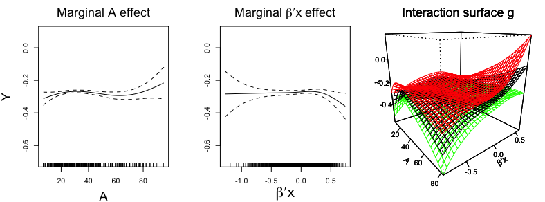
Figure 1: The first two panels: the marginal effect of dose $A$ (left panel) and that of the estimated single-index (middle panel) with 95% confidence bands (dashed curves) given the estimated $\beta^{\top}X$. The third panel: the estimated link surface $(g)$ for the dose ($A$) and index ($\beta^{\top}X$) interaction; the red and green surfaces are at $\pm 2$ standard error from the estimated surface (the black) in the middle, conditioning on the estimated single-index.

To evaluate the performance of the individualized dose rules estimated from the $6$ methods, including the propensity score-adjusted outcome-weighted learning with a linear/Gaussian kernel, denoted as L-O-learning(Prp) and K-O-learning(Prp), respectively) considered in Section 5, we randomly split the dataset at a ratio of 1-to-1 into a training set and a testing set, replicated 100 times, each time estimating $f_{\mathrm{opt}}$ using the $6$ methods based on the training set, and estimating the value (1) of each estimated $f_{\mathrm{opt}}$ based on the testing set. Unlike the simulated data in Section 5, the true relationship between the covariate-specific dose and the response is unknown. Therefore, for each dose rule $f$, we need to estimate the value (1) from the testing data. Given a dose rule $f$, only a very small proportion (or none) of the observations will satisfy $A_{i}=f(X_{i})$, and thus only a very small proportion (or none) of the observations in the testing data will contribute information to estimate the value (1). However, Cai and Tian (2016) noted that the value (1) for each $f$ can also be written as $\mathcal{V}(f)=\mathbb{E}[\mathbb{E}[Y|A=f(X),f(X)]]$. Therefore, using a $2$-dimensional smoother of $A$ and $f(X)$ for $Y$, one may first obtain a nonparametric estimate of $\mathbb{E}[Y|A,f(X)]$, denoted as $\hat{m}({A,f(X)})$, and then $\mathcal{V}(f)$ may be estimated as $\hat{\mathcal{V}}(f)=n^{-1}\sum_{i=1}^{n}\hat{m}({f(X_{i}),f(X_{i})})$. Specifically, given a dose rule $f$ estimated from a training set, we can estimate $\mathbb{E}[Y|A,f(X)]$ based on $(Y_{i},A_{i},f(X_{i}))$ from a test set, using a set of thin plate regression spline bases obtained from a rank-100 eigen-approximation to a thin plate spline, with the smoothness parameter selected by REML, implemented via the R (R Core Team, 2019) function mgcv::gam (Wood, 2019). A thin plate spline is an isotropic smooth; isotropy is often appropriate for two variables observed on the same scale, which is the case here.

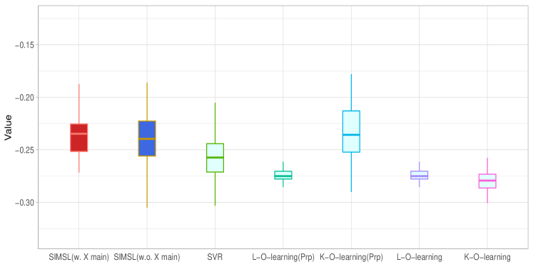
Figure 2: Boxplots of the estimated values of the individualized dose rules using $7$ approaches, obtained from $100$ randomly split testing sets. Mean (and standard deviation) of the value estimates: SIMSL(w. $X$ main): -0.233 (0.03); SIMSL(w.o. $X$ main): -0.237 (0.03); SVR: -0.256 (0.02); L-O-learning(Prp): -0.274 (0.01); K-O-learning(Prp): -0.234 (0.03); L-O-learning: -0.274 (0.01); K-O-learning: -0.279 (0.01).

Figure 2 displays a boxplot describing the distributions for the estimated values (1) of “SIMSL(w. $X$ main)” (SIMSL incorporating $\mu$ in the estimation) and “SIMSL(w.o. $X$ main)” (SIMSL without incorporating $\mu$ in the estimation), and the other five estimation methods described in Section 5, obtained from the aforementioned $100$ random training/testing splits. The boxplots indicate that the proposed SIMSL methods (note that SIMSL(w. $X$ main) slightly outperforms SIMSL(w.o. $X$ main)) and the propensity-score adjusted K-O-learning of Chen et al. (2016) perform at a similar level, while outperforming all other approaches. The results illustrate the potential utility of the proposed regression approach to optimizing individualized dose rules. In comparison to the outcome-weighted learning approach of Chen et al. (2016), one advantage of the proposed approach is that it allows visualization of the estimated interactive structure on the dose-index domain as illustrated in the right panel of Figure 3. Additionally, if each of the covariates is standardized to have, say, unit variance, then the relative importance of each covariate in characterizing the heterogeneous dose response can be determined by the magnitude of the estimated coefficients in $\beta$, rendering a potentially useful interpretation when examining the drug-covariates interactions.

7 Discussion

In this paper, we proposed a variant of a single-index model that utilizes a surface link-function as a function of a linear projection of covariates and a continuous “treatment” variable. This single index model with a surface link can effectively estimate the effect on a response of possibly nonlinear interactions between a set of covariates and the treatment variable defined on a continuum. The proposed regression model is useful for developing personalized dose rules in precision medicine, and more generally, in a situation where we are particularly interested in modeling interactions between a vector of covariates and a real-valued predictor of interest. The model gives an intuitive method for modeling such interactions, without the need for a significant change in the established generalized additive regression modeling framework.

One important limitation is that the confidence band associated with the estimated surface $g$ is computed conditional on the estimated $\beta^{\top}X$, and the uncertainty in $\beta$ is not accounted for. The fact that the domain of $g$ varies depending on the estimate of $\beta$ complicates the confidence band construction for $g$. One potential solution would be to consider a Bayesian approach and use a posterior distribution of $g(\beta^{\top}X,A)$, and make probabilistic statements about the prediction given $(X,A)$.

Depending on context, for scientific interpretability of the model, it may be sometimes desirable to consider shape constraints such as monotonicity or convexity/concavity (see Supplementary Materials Section C.4 for some discussion on this topic). The development of a Bayesian framework for this regression model, with potential monotonicity or convexity/concavity constraints on the link surface is currently under investigation. In many applications, only a subset of variables may be useful in determining an optimal individualized dose rule. Also, high-dimensional settings can lead to instabilities and issues of overfitting. Forthcoming work will introduce a regularization method that can both avoid overfitting and choose among multiple potential covariates by obtaining a sparse estimate of the single-index coefficient $\beta$. Future extensions of this work could also include an extension to incorporate a functional covariate.

SUPPLEMENTAL MATERIALS

Supplementary Materials:

a pdf file containing the proof of Proposition 1, a data analysis example and additional simulations illustrating an application of the generalized single-index regression approach described in Section 4.

R-package for SIMSL routine:

R-package simsl (Park et al., 2021) available on CRAN containing code to perform the proposed single-index regression method, and the datasets and the simulation examples illustrated in this article. For the case of discrete-valued treatments, we refer to R-package simml (Park et al., 2019).

References

- Cai and Tian (2016) Cai, T. and Tian, L. (2016). Comment: Personalized dose finding using outcome weighted learning. Journal of the American Statistical Association 111:1521–1524.
- Chen et al. (2016) Chen, G., Zeng, D., and Kosorok, M. R. (2016). Personalized dose finding using outcome wieghted learning. Journal of the American Statistical Association 111:1509–1547.
- Chen et al. (2020) Chen, H., Lu, W., and Song, R. (2020). Statistical inference for online decision making: In a contextual bandit setting. Journal of the American Statistical Association. doi:10.1080/01621459.2020.1770098 .
- de Boor (2001) de Boor, C. (2001). A Practical Guide to Splines. Springer-Verlag, New York.
- Dudík et al. (2014) Dudík, M., Erhan, D., Langford, J., and Li, L. (2014). Doubly robust policy evaluation and optimization. Statistical Science 29:485–511.
- Eilers and Marx (2003) Eilers, P. and Marx, B. (2003). Multivariate calibration with temperature interaction using 2-dimensional penalized signal regression. Chemometrics and Intellegence Laboratory Systems 66:159–174.
- Gunter et al. (2011) Gunter, L., Zhu, J., and Murphy, S. (2011). Variable selection for qualitative interactions in presonalized medicine while controlling the family-wise error rate. Journal of Biopharmaceutical Statistics 21:1063–1078.
- Hastie and Tibshirani (1999) Hastie, T. and Tibshirani, R. (1999). Generalized Additive Models. Chapman & Hall Ltd.
- International Warfarin Pharmacogenetics Consortium et al. (2009) International Warfarin Pharmacogenetics Consortium, Klein, T., Altman, R., Eriksson, N., Gage, B., Kimmel, S., Lee, M., Limdi, N., Page, D., Roden, D., Wagner, M., Caldwell, M., and Johnson, J. (2009). Estimation of the warfarin dose with clinical and pharmacogenetic data. The New England Journal of Medicine 360:753–674.
- Jun et al. (2017) Jun, K. S., Bhargava, A., Nowak, R., and Willett, R. (2017). Scalable generalized linear bandits: Online computation and hashing. In Advances in Neural Information Processing Systems 30:99–109.
- Kaelbling et al. (1996) Kaelbling, L., Littman, M., and Moore, A. (1996). Reinforcement learning: a survey. Journal of Artificial Intellegence Research 4:237–285.
- Kallus and Zhou (2018) Kallus, N. and Zhou, A. (2018). Policy evaluation and optimization with continuous treatments. In International Conference on Artificial Intelligence and Statistics 84:1243–1251.
- Kennedy et al. (2017) Kennedy, E. H., Ma, Z., McHugh, M. D., and Small, D. S. (2017). Nonparametric methods for doubly robust estimation of continuous treatment effects. Journal of Royal Statistical Society: Series B 79:1229–1245.
- Kleinberg et al. (2019) Kleinberg, R., Slivkins, A., and Upfal, E. (2019). Bandits and experts in metric spaces. Journal of the ACM 66:77.
- Krishnamurthy et al. (2020) Krishnamurthy, A., Langford, J., Slivkins, A., and Zhang, C. (2020). Contextual bandits with continuous actions: Smoothing, zooming, and adapting. Journal of Machine Learning Research 21:1–45.
- Kveton et al. (2020) Kveton, B., Zaheer, M., Szepesvari, C., Li, L., Ghavamzadeh, M., and Boutilier, C. (2020). Randomized exploration in generalized linear bandits. Proceedings of the 23rd International Conference on Artificial Intelligence and Statistics 108:2066–2076.
- Laber and Zhao (2015) Laber, E. B. and Zhao, Y. (2015). Tree-based methods for individualized treatment regimes. Biometrika 102:501–514.
- Lattimore and Szepesvari (2019) Lattimore, T. and Szepesvari, C. (2019). Bandit algorithms. Cambridge University Press.
- Li et al. (2017) Li, L., Lu, Y., and Zhou, D. (2017). Provably optimal algorithms for generalized linear contextual bandits. In Proceedings of the 34th International Conference on Machine Learning 70:2071–2080.
- Lu et al. (2010) Lu, T., Pal, D., and Pal, M. (2010). Contextual multi-armed bandits. Proceedings of the Thirteenth International Conference on Artificial Intelligence and Statistics, JMLR Workshop and Conference Proceedings 9:485–492.
- Lu et al. (2013) Lu, W., Zhang, H., and Zeng, D. (2013). Variable selection for optimal treatment decision. Statistical Methods in Medical Research 22:493–504.
- Majzoubi et al. (2020) Majzoubi, M., Zhang, C., Chari, R. K., A. Langford, J., and Slivkins, A. (2020). Efficient contextual bandits with continuous actions. ArXiv, abs/2006.06040 .
- Marx (2015) Marx, B. (2015). Varying-coefficient single-index signal regression. Chemometrics and Intellegence Laboratory Systems 143:111–121.
- Murphy (2003) Murphy, S. A. (2003). Optimal dynamic treatment regimes. Journal of the Royal Statistical Society: Series B (Statistical Methodology) 65:331–355.
- Park et al. (2019) Park, H., Petkova, E., Tarpey, T., and Ogden, R. (2019). simml: Single-index models with multiple-links. R package version 0.1.0 .
- Park et al. (2021) Park, H., Petkova, E., Tarpey, T., and Ogden, R. (2021). simsl: Single-index models with a surface-link. R package version 0.1.1 .
- Park et al. (2020) Park, H., Petkova, E., Tarpey, T., and Ogden, R. T. (2020). A constrained single-index regression for estimating interactions between a treatment and covariates. Biometrics. doi:10.1111/biom.13320 .
- Perchet and Rigollet (2013) Perchet, V. and Rigollet, P. (2013). The multi-armed bandit problem with covariates. The Annals of Statistics 41:693–721.
- Qian and Murphy (2011) Qian, M. and Murphy, S. A. (2011). Performance guarantees for individualized treatment rules. The Annals of Statistics 39:1180–1210.
- R Core Team (2019) R Core Team (2019). R: A Language and Environment for Statistical Computing. R Foundation for Statistical Computing, Vienna, Austria.
- Rich et al. (2014) Rich, B., Moodie, E. E., and Stephens, D. A. (2014). Simulating sequential multiple assignment randomized trials to generate optimal personalized warfarin dosing strategies. Clinical Trials 11:435–444.
- Robins (2004) Robins, J. (2004). Optimal Structural Nested Models for Optimal Sequential Decisions. Springer, New York.
- Schulz and Moodie (2020) Schulz, J. and Moodie, E. E. (2020). Doubly robust estimation of optimal dosing strategies. Journal of the American Statistical Association. doi:10.1080/01621459.2020.1753521 .
- Slivkins (2014) Slivkins, A. (2014). Contextual bandits with similarity information. Journal of Machine Learning Research 15:2533–2568.
- Smola and Scholopf (2004) Smola, A. and Scholopf, B. (2004). A tutorial on support vector regression. Statistics and Computing 14:199–222.
- Tian et al. (2014) Tian, L., Alizadeh, A., Gentles, A., and Tibshrani, R. (2014). A simple method for estimating interactions between a treatment and a large number of covariates. Journal of the American Statistical Association 109:1517–1532.
- Vapnik (1995) Vapnik, V. N. (1995). The Nature of Statistical Learning Theory, volume 8. Springer, New York.
- Wood (2006) Wood, S. N. (2006). Low-rank scale-invariant tensor product smooths for generalized additive mixed models. Biometrics 62:1025–1036.
- Wood (2017) Wood, S. N. (2017). Generalized Additive Models: An Introduction with R. Chapman & Hall/CRC, second edition.
- Wood (2019) Wood, S. N. (2019). mgcv: Mixed GAM computation vehicle with automatic smoothness estimation. R package version 1.8.28 .
- Zhang et al. (2012) Zhang, B., Tsiatis, A. A., Davidian, M., Zhang, M., and Laber, E. (2012). Estimating optimal treatment regimes from classification perspective. Stat 1:103–114.
- Zhao et al. (2009) Zhao, Y., Kosorok, M., and Zeng, D. (2009). Reinforcement learning design for cancer clinical trials. Statistics in Medicine 28:3294–3315.
- Zhao et al. (2012) Zhao, Y., Zeng, D., Rush, A. J., and Kosorok, M. R. (2012). Estimating individualized treatment rules using outcome weighted learning. Journal of the American Statistical Association 107:1106–1118.
- Zhou et al. (2020) Zhou, W., Zhu, R., and Zeng, D. (2020). A parsimonious personalized dose-finding model via dimension reduction. Biometrika. doi:10.1093/biomet/asaa087 .
- Zhu et al. (2020) Zhu, L., Lu, W., Kosorok, M. R., and Song, R. (2020). Kernel assisted learning for personalized dose finding. arXiv:2007.09811 .