A constrained sparse additive model for treatment effect-modifier selection

Abstract

Sparse additive modeling is a class of effective methods for performing high-dimensional nonparametric regression. This paper develops a sparse additive model focused on estimation of treatment effect-modification with simultaneous treatment effect-modifier selection. We propose a version of the sparse additive model uniquely constrained to estimate the interaction effects between treatment and pretreatment covariates, while leaving the main effects of the pretreatment covariates unspecified. The proposed regression model can effectively identify treatment effect-modifiers that exhibit possibly nonlinear interactions with the treatment variable, that are relevant for making optimal treatment decisions. A set of simulation experiments and an application to a dataset from a randomized clinical trial are presented to demonstrate the method. Individualized treatment rules; Sparse additive models; Treatment effect-modifiers

1 Introduction

Identification of patient characteristics influencing treatment responses, which are often termed treatment effect-modifiers or treatment effect-moderators, is a top research priority in precision medicine. In this paper, we develop a flexible yet simple and intuitive regression approach to identifying treatment effect-modifiers from a potentially large number of pretreatment patient characteristics. In particular, we utilize a sparse additive model (Ravikumar and others, 2009) to conduct effective treatment effect-modifier selection.

The clinical motivation behind the development of a high-dimensional additive regression model that can handle a large number of pretreatment covariates, specifically designed to model treatment effect-modification and variable selection, is a randomized clinical trial (Trivedi and others, 2016) for treatment of major depressive disorder. A large number of baseline patient characterisitics were collected from each participant prior to randomization and treatment allocation. The primary goal of this study is to discover biosignatures of heterogeneous treatment response. As we move towards optimizing treatment decisions for individual patients, discovering and identifying which pretreatment patient characteristics influence treatment effects has the potential to significantly enhance clinical reasoning in practice (see, e.g., Royston and Sauerbrei, 2008).

The major challenge in efficiently modeling treatment effect-modification from a randomized clinical trial dataset is that variability due to treatment effect modification (i.e., the treatment-by-covariates interaction effects on outcomes) is typically dwarfed by a relatively large degree of non-treatment-related variability (i.e., the main effects of the pretreatment covariates on treatment outcomes). In particular, in regression, due to potential confounding between the main effect of the covariates and the treatment-by-covariates interaction effect, misspecification of the covariate main effect may significantly influence estimation of the treatment-by-covariates interaction effect.

A simple and elegant linear model-based approach to modeling the treatment-by-covariates interactions, termed the modified covariate (MC) method, that is robust against model misspecification of the covariates’ main effects was developed by Tian and others (2014). The method utilizes a simple parameterization and bypasses the need to model the main effects of the covariates. See also Murphy (2003); Lu and others (2011); Shi and others (2016); Jeng and others (2018) for the similar linear model-based approaches to estimating the treatment-by-covariates interactions. However, these approaches assume a stringent linear model to specify the treatment-by-covariates interaction effects, and are limited to the binary-valued treatment variable case only. In this work, we extend the optimization framework of Tian and others (2014) for modeling the treatment-by-covariates interactions using a more flexible regression setting based on additive models (Hastie and Tibshirani, 1999) that can accommodate more than two treatment conditions, while allowing an unspecified main effect of the covariates. Additionally, via an appropriate regularization, the proposed approach simultaneously achieves treatment effect-modifier selection in estimation.

In Section 2, we introduce an additive model that has both the unspecified main effect of the covariates and the treatment-by-covariates interaction effect additive components. Then we develop an optimization framework specifically targeting the interaction effect additive components of the model, with a sparsity-inducing regularization parameter to encourage sparsity in the set of component functions. In Section 3, we develop a coordinate decent algorithm to estimate the interaction effect part of the model and consider an optimization strategy for estimating individualized treatment rules. In Section 4, we illustrate the performance of the method in terms of treatment effect-modifier selection and estimation of optimal individualized treatment rules through simulation examples. Section 5 provides an illustrative application from a depression clinical trial, and the paper concludes with discussion in Section 6.

2 Models

Let $A\in\{1,\ldots,L\}$ denote a treatment variable assigned with associated probabilities $(\pi_{1},\ldots,\pi_{L})$, $\sum_{a=1}^{L}\pi_{a}=1$, and $\pi_{a}>0$, and let $\bm{X}=(X_{1},\ldots,X_{p})^{\top}\in\mathbb{R}^{p}$ denote pretreatment covariates, independent of $A$ (as in the case of a randomized trial). If the treatment assignment depends on the covariates, then the probabilities $\{\pi_{a}\}_{a\in\{1,\ldots,L\}}$ can be replaced by propensity scores $\{\pi_{a}(\bm{X})\}_{a\in\{1,\ldots,L\}}$ which would typically need to be estimated from data. We let $Y^{(a)}\in\mathbb{R}$ (a = 1,…,L) be the potential outcome if the patient received treatment $A=a$ $(a=1,\ldots,L)$; we only observe $Y=Y^{(A)}$, $A$ and $\bm{X}$.

Throughout the paper, we assume that $\mathbb{E}[Y|A=a]=0\ (a=1,\ldots,L)$, without loss of generality, i.e., the main effect of $A$ on the outcome is centered at $0$. This is only to suppress the treatment $a$-specific intercepts in regression models in order to simplify the exposition, and can be achieved by removing the treatment level $a$-specific means from $Y\in\mathbb{R}$. We model the treatment outcome $Y$ by the following additive model:

$$\mathbb{E}[Y|\bm{X},A=a]=\underbrace{\mu^{\ast}(\bm{X})}_{\bm{X}\mbox{ ``main'' effect}}+\underbrace{\sum_{j=1}^{p}g_{j,a}^{\ast}(X_{j})}_{A\mbox{-by-}\bm{X}\mbox{ interactions}}\quad(a=1,\ldots,L)$$ (1)

In model (1), the first term $\mu^{\ast}(\bm{X})$ does not depend on the treatment variable $A$ and thus the $A$-by-$\bm{X}$ interaction effects are determined only by the second component $\sum_{j=1}^{p}g_{j,A}^{\ast}(X_{j})$. In terms of modeling treatment effect-modification, the term $\sum_{j=1}^{p}g_{j,A}^{\ast}(X_{j})$ in (1) corresponds to the “signal” component, whereas the term $\mu^{\ast}(\bm{X})$ corresponds to a “nuisance” component.

In (1), for each individual covariate $X_{j}$, we utilize a treatment $a$-specific smooth $g_{j,a}^{\ast}$ separately for each treatment condition $a\in\{1,\ldots,L\}$. However, it is useful to treat the set of treatment-specific smooths for $X_{j}$ as a single unit, i.e., a single component function $g_{j}^{\ast}=\{g_{j,a}^{\ast}\}_{a\in\{1,\ldots,L\}}$, for the purpose of treatment effect-modifier variable selection.

In model (1), to separate $\mu^{\ast}(\bm{X})$ from the component $\sum_{j=1}^{p}g_{j,a}^{\ast}(X_{j})$ and obtain an identifiable representation, without loss of generality, we assume that the set of treatment $a$-specific smooths $\{g^{\ast}_{j,a}\}_{a\in\{1,\ldots,L\}}$ of the $j$th component function $g_{j,A}^{\ast}(X_{j})$ satisfies a condition:

$$\mathbb{E}[g_{j,A}^{\ast}(X_{j})|X_{j}]=\sum_{a=1}^{L}\pi_{a}g_{j,a}^{\ast}(X_{j})=0\quad\mbox{almost surely,}\quad(j=1,\ldots,p).$$ (2)

Condition (2) implies $\mathbb{E}\big{[}\sum_{j=1}^{p}g_{j,A}^{\ast}(X_{j})|\bm{X}\big{]}=0$ almost surely, and separates the $A$-by-$\bm{X}$ interaction effect component, $\sum_{j=1}^{p}g_{j,a}^{\ast}(X_{j})$, from the $\bm{X}$ “main” effect component, $\mu^{\ast}(\bm{X})$, in model (1). For model (1), we assume $Y=\mathbb{E}[Y|\bm{X},A]+\epsilon$, where $\epsilon$ is a zero-mean noise with finite variance, independent of $\bm{X}$ and $A$.

Notation: For a single component $j$ and general (measurable) component functions $g_{j}=\{g_{j,a}\}_{a\in\{1,\ldots,L\}}$, define the $L^{2}$ norm of $g_{j}$ as $\lVert g_{j}\rVert\ =\ \sqrt{\mathbb{E}\big{[}g_{j,A}^{2}(X_{j})\big{]}}$, where expectation is taken with respect to the joint distribution of $(A,X_{j})$. (When there is no confusion, we also use $\lVert\cdot\rVert$ to denote the $L^{2}$ norm of a real vector.) For a set of random variables $(A,X_{j})$, let $\mathcal{H}_{j}=\{g_{j}\mid\mathbb{E}[g_{j,A}(X_{j})]=0,\lVert g_{j}\rVert<\infty\}$ with inner product on the space defined as $\langle g_{j},f_{j}\rangle=\mathbb{E}[g_{j,A}(X_{j}),f_{j,A}(X_{j})]$. Sometimes we also write $g_{j}:=g_{j,A}(X_{j})$ for the notational simplicity.

Under model (1) subject to (2), the component functions $\{g_{j}^{\ast},j=1,\ldots,p\}$ associated with the $A$-by-$\bm{X}$ interaction effect can be viewed as the solution to the constrained optimization:

$$\{g_{j}^{\ast}\}\quad= \underset{\{g_{j}\in\mathcal{H}_{j}\}}{\text{argmin}} E\bigg{[}\big{\{}Y-\mu^{\ast}(\bm{X})-\sum_{j=1}^{p}g_{j,A}(X_{j})\big{\}}^{2}\bigg{]}$$ (3)

subject to $$\mathbb{E}[g_{j,A}(X_{j})|X_{j}]=0\quad(j=1,\ldots,p),$$

where $\mu^{\ast}(\bm{X})$ is given from the assumed model (1) (and is considered as fixed in (3)). Since the minimization in (3) is in terms of $\{g_{j}\in\mathcal{H}_{j},j=1,\ldots,p\}$, the objective function part of the right-hand side of (3) can be reduced to:

$$\operatorname*{arg\,min}_{\{g_{j}\in\mathcal{H}_{j}\}}\ \mathbb{E}\bigg{[}Y^{2}+\big{\{}\sum_{j=1}^{p}g_{j,A}(X_{j})\big{\}}^{2}-2\big{\{}\sum_{j=1}^{p}g_{j,A}(X_{j})\big{\}}Y+2\big{\{}\sum_{j=1}^{p}g_{j,A}(X_{j})\big{\}}\mu^{\ast}(\bm{X})\bigg{]}$$

$$= \operatorname*{arg\,min}_{\{g_{j}\in\mathcal{H}_{j}\}}\ \mathbb{E}\bigg{[}Y^{2}+\big{\{}\sum_{j=1}^{p}g_{j,A}(X_{j})\big{\}}^{2}-2\big{\{}\sum_{j=1}^{p}g_{j,A}(X_{j})\big{\}}Y+2\mu^{\ast}(\bm{X})\mathbb{E}\bigg{[}\sum_{j=1}^{p}g_{j,A}(X_{j})|\bm{X}\bigg{]}\bigg{]}$$

$$= \operatorname*{arg\,min}_{\{g_{j}\in\mathcal{H}_{j}\}}\ \mathbb{E}\bigg{[}Y^{2}+\big{\{}\sum_{j=1}^{p}g_{j,A}(X_{j})\big{\}}^{2}-2\big{\{}\sum_{j=1}^{p}g_{j,A}(X_{j})\big{\}}Y\bigg{]},$$

where the second line is from an application of the iterated expectation rule conditioning on $\bm{X}$ and the third line follows from the constraint $\mathbb{E}[g_{j,A}(X_{j})|X_{j}]=0$ $(j=1,\ldots,p)$ on the right-hand side of (3). Therefore, representation (3) can be simplified to:

$$\{g_{j}^{\ast}\}\quad= \underset{\{g_{j}\in\mathcal{H}_{j}\}}{\text{argmin}} \mathbb{E}\bigg{[}\big{\{}Y-\sum_{j=1}^{p}g_{j,A}(X_{j})\big{\}}^{2}\bigg{]}$$ (4)

subject to $$\mathbb{E}[g_{j,A}(X_{j})|X_{j}]=0\quad(j=1,\ldots,p),$$

Representation (4) of the component functions $\{g_{j}^{\ast},j=1,\ldots,p\}$ of the underlying model (1) is particularly useful when the (high-dimensional) “nuisance” function $\mu^{\ast}$ in (1) is complicated and prone to specification error. Note,

$$\mathbb{E}\bigg{[}\mu^{\ast}(\bm{X})\sum_{j=1}^{p}g_{j,A}\big{(}X_{j}\big{)}\bigg{]}=\mathbb{E}\bigg{[}\mu^{\ast}(\bm{X})\sum_{j=1}^{p}\mathbb{E}\big{[}g_{j,A}\big{(}X_{j}\big{)}|\bm{X}\big{]}\bigg{]}=0,$$ (5)

indicating that the component $\sum_{j=1}^{p}g_{j,A}\big{(}X_{j}\big{)}\in\mathcal{H}_{1}+\cdots+\mathcal{H}_{p}$ (subject to the identifiability constraint $\mathbb{E}[g_{j,A}(X_{j})|X_{j}]=0$) is structured to be orthogonal to the $\bm{X}$ main effect $\mu^{\ast}(\bm{X})$. This orthogonality property is useful for estimating the additive model $A$-by-$\bm{X}$ interaction effect $\sum_{j=1}^{p}g_{j,A}^{\ast}(X_{j})$, in the presence of the unspecified $\mu^{\ast}(\bm{X})$ of model (1).

Under model (1), the potential treatment effect-modifiers among $\{X_{j},j=1,\ldots,p\}$ enter the model only through the interaction effect term $\sum_{j=1}^{p}g_{j,A}^{\ast}(X_{j})$ that associates the treatment $A$ to the treatment outcome $Y$. Ravikumar and others (2009) proposed sparse additive modeling (SAM) for component selection in high-dimensional additive models with a large $p$. As in SAM, to deal with a large $p$ and to achieve treatment effect-modifier selection, we impose sparsity on the set of component functions $\{g_{j}^{\ast},j=1,\ldots,p\}$ associated with the interaction effect term of model (1), under the often practical and reasonable assumption that most covariates are irrelevant as treatment effect-modifiers. This sparsity structure on the index set $\{j\}$ for the nonzero component functions $\{g_{j}^{\ast}:g_{j}^{\ast}\neq 0\}$ can be usefully incorporated into the optimization-based criterion (4) in representing $\{g_{j}^{\ast}\}$:

$$\{g_{j}^{\ast}\}\quad= \underset{\{g_{j}\in\mathcal{H}_{j}\}}{\text{argmin}} \mathbb{E}\bigg{[}\big{\{}Y-\sum_{j=1}^{p}g_{j,A}(X_{j})\big{\}}^{2}\bigg{]}\ +\ \lambda\sum_{j=1}^{p}\lVert g_{j}\rVert$$ (6)

subject to $$\mathbb{E}[g_{j,A}(X_{j})|X_{j}]=0\quad(j=1,\ldots,p),$$

for a sparsity-inducing parameter $\lambda\geq 0$. The term $\sum_{j=1}^{p}\lVert g_{j}\rVert$ in (6) behaves like an $L^{1}$ ball across different components $\{g_{j},j=1,\ldots,p\}$ to encourage sparsity in the set of component functions. For example, a large value of $\lambda$ on the right-hand side of (6) will generate a sparse solution with many component functions $g_{j}^{\ast}$ on the left-hand side set exactly to zero.

3 Estimation

3.1 Model estimation

For each $j$, the minimizer $g_{j}^{\ast}$ of the optimization problem (6) has a component-wise closed-form expression.

Theorem 3.1.

Given $\lambda\geq 0$, the minimizer $g_{j}^{\ast}\in\mathcal{H}_{j}$ of (6) satisfies:

$$g_{j,A}^{\ast}(X_{j})\ =\ \left[1-\frac{\lambda}{\lVert f_{j}\rVert}\right]_{+}f_{j,A}(X_{j})\quad\mbox{almost surely},$$ (7)

where

$$f_{j,A}(X_{j})\ =\ \mathbb{E}[R_{j}|X_{j},A]\ -\ \mathbb{E}[R_{j}|X_{j}],$$ (8)

in which

$$R_{j}=Y-\sum_{j^{\prime}\neq j}g_{j^{\prime},A}^{\ast}(X_{j^{\prime}})$$ (9)

represents the $j$th partial residual. In (7), $Z_{+}=\max(0,Z)$ represents the positive part of $Z$.

Note that the $f_{j,A}(X_{j})$ correspond to the projections of $R_{j}$ onto $\mathcal{H}_{j}$ subject to the constraint in (6). The proof of Theorem 3.1 is in the Supplementary Materials.

The component-wise expression (7) for $g_{j}^{\ast}$ suggests that we can employ a coordinate descent algorithm (e.g., Tseng, 2001) to solve (6). Given a sparsity parameter $\lambda\geq 0$, we can use a standard backfitting algorithm used in fitting additive models (Hastie and Tibshirani (1999)) that fixes the set of current approximates for $g_{j^{\prime}}^{\ast}$ at all $j^{\prime}\neq j$, and obtains a new approximate of $g_{j}^{\ast}$ by equation (7), and iterates through all $j$ until convergence. A sample version of the algorithm can be obtained by inserting sample estimates into the population expressions (9), (8) and (7) for each coordinate $j$, which we briefly describe next.

Given data $(X_{ij},A_{i})$ $(i=1,\ldots,n;j=1,\dots,p)$, for each $j$, let $\hat{R}_{j}=Y-\sum_{j^{\prime}\neq j}\hat{g}_{j^{\prime},A}^{\ast}(X_{j^{\prime}})$, corresponding to the data-version of the $j$th partial residual $R_{j}$ in (9), where $\hat{g}_{j^{\prime}}^{\ast}$ represents a current estimate for $g_{j^{\prime}}^{\ast}$. We estimate $g_{j}^{\ast}$ in (7) in two steps: 1) estimate the function $f_{j}$ in (8); 2) plug the estimate of $f_{j}$ into $\left[1-\frac{\lambda}{\lVert f_{j}\rVert}\right]_{+}$ in (7), to obtain the soft-thresholded estimate $\hat{g}_{j}^{\ast}$.

Although any linear smoothers can be utilized to obtain the estimators $\{\hat{g}_{j}^{\ast}\}$ as described in Remark 1 at the end of this section, in this paper, we shall focus on regression spline-type estimators which are particularly simple and computationally efficient to implement. Specifically, for each $j$, the function $g_{j}\in\mathcal{H}_{j}$ on the right-hand side of (6) will be represented by:

$$g_{j,a}(X_{j})=\bm{\Psi}_{j}(X_{j})^{\top}\bm{\theta}_{j,a}\quad(a=1,\ldots,L)$$ (10)

for some prespecified $d_{j}$-dimensional basis $\bm{\Psi}_{j}(\cdot)\in\mathbb{R}^{d_{j}}$ (e.g., $B$-spline basis on evenly spaced knots on a bounded range for $X_{j}$) and a set of unknown treatment $a$-specific basis coefficients $\{\bm{\theta}_{j,a}\in\mathbb{R}^{d_{j}}\}_{a\in\{1,\ldots,L\}}$. Given representation (10) for the component function $g_{j}$, the constraint $\mathbb{E}[g_{j,A}(X_{j})|X_{j}]=0$ in (6) can be simplified to $\mathbb{E}[\bm{\theta}_{j,A}]=\sum_{a=1}^{L}\pi_{a}\bm{\theta}_{j,a}=\bm{0}$. This constraint can be written succinctly in a matrix form as

$$\bm{\pi}^{(j)}\bm{\theta}_{j}=\bm{0},$$ (11)

where $\bm{\theta}_{j}:=(\bm{\theta}_{j,1}^{\top},\bm{\theta}_{j,2}^{\top},\ldots,\bm{\theta}_{j,L}^{\top})^{\top}\in\mathbb{R}^{d_{j}L}$ is the vectorized version of the basis coefficients $\{\bm{\theta}_{j,a}\}_{a\in\{1,\ldots,L\}}$ in (10), and the $d_{j}\times d_{j}L$ matrix $\bm{\pi}^{(j)}:=\left(\pi_{1}\bm{I}_{d_{j}};\pi_{2}\bm{I}_{d_{j}};\ldots;\pi_{L}\bm{I}_{d_{j}}\right)$ where $\bm{I}_{d_{j}}$ denotes the $d_{j}\times d_{j}$ identity matrix.

The restriction of the function $g_{j}$ to the form (10) restricts also the minimizer $g_{j}^{\ast}$ in (7) (note, $g_{j,A}^{\ast}(X_{j})=s_{j}^{(\lambda)}f_{j,A}(X_{j})$, where $s_{j}^{(\lambda)}=\left[1-\lambda/\lVert f_{j}\rVert\right]_{+}$) to the form (10). In particular, we can express the function $f_{j}$ in (8) as:

$$f_{j,A}(X_{j}) =\mathbb{E}[R_{j}|X_{j},A]-\sum_{a=1}^{L}\pi_{a}\mathbb{E}[R_{j}|X_{j},A=a]$$ (12)

$$=\bm{\Psi}_{j}(X_{j})\bm{\theta}_{j,A}^{\ast}-\bm{\Psi}_{j}(X_{j})\big{(}\sum_{a=1}^{L}\pi_{a}\bm{\theta}_{j,a}^{\ast}\big{)}$$

where $\{\bm{\theta}_{j,a}^{\ast}\}_{a\in\{1,\ldots,L\}}:=\underset{\{\bm{\theta}_{j,a}\in\mathbb{R}^{d_{j}}\}}{\text{argmin}}\mathbb{E}\big{[}\{R_{j}-\bm{\Psi}_{j}(X_{j})^{\top}\bm{\theta}_{j,A}\}^{2}\big{]}$. The first term $\mathbb{E}[R_{j}|X_{j},A]$ in (12) corresponds to the $L^{2}$ projection of the $j$th partial residual $R_{j}$ onto the class of functions of the form (10) (without the imposition of the constraint (11)), whereas the second term $-\sum_{a=1}^{L}\pi_{a}\mathbb{E}[R_{j}|X_{j},A=a]$ centers the first term to satisfy the linear constraint (11). It is straightforward to verify that $f_{j}$, as given in (12), corresponds to the $L^{2}$ projection of $R_{j}$ onto the subspace of measurable functions of the form (10) subject to the linear constraint (11).

Let the $n\times d_{j}$ matrices $\bm{D}_{j,a}$ $(a=1,\ldots,L)$ denote the evaluation matrices of the basis function $\bm{\Psi}_{j}(\cdot)$ on $X_{ij}$ $(i=1,\ldots,n)$ specific to the treatment $A=a$ $(a=1,\ldots,L)$, whose $i$th row is the $1\times d_{j}$ vector $\bm{\Psi}_{j}(X_{ij})^{\top}$ if $A_{i}=a$, and a row of zeros $\bm{0}^{\top}$ if $A_{i}\neq a$. Then the column-wise concatenation of the design matrices $\{\bm{D}_{j,a}\}_{a\in\{1,\ldots,L\}}$, i.e., the $n\times d_{j}L$ matrix $\bm{D}_{j}=(\bm{D}_{j,1};\bm{D}_{j,2};\ldots;\bm{D}_{j,L})$, defines the model matrix associated with the vectorized model coefficient $\bm{\theta}_{j}\in\mathbb{R}^{d_{j}L}$, vectorized across $\{\bm{\theta}_{j,a}\}_{a\in\{1,\ldots,L\}}$ in representation (10). Then we can represent the function $g_{j,A}(X_{j})$ in (10), based on the sample data, by the length-$n$ vector:

$$\bm{g}_{j}=\bm{D}_{j}\bm{\theta}_{j}$$ (13)

subject to the linear constraint (11).

When computing the data version of the function $f_{j}$ in (8) which corresponds to the projection of $R_{j}$ onto the functional class of (10) subject to (11), the linear constraint (11) on $\bm{\theta}_{j}$ can be conveniently absorbed into the model matrix $\bm{D}_{j}$ in (13) by reparametrization, as we describe next. We can find a $d_{j}L\times d_{j}(L-1)$ basis matrix $\bm{Z}^{(j)}$, such that if we set $\bm{\theta}_{j}=\bm{Z}^{(j)}\tilde{\bm{\theta}}_{j}$ for any arbitrary vector $\tilde{\bm{\theta}}_{j}\in\mathbb{R}^{d_{j}(L-1)}$, then the vector $\bm{\theta}_{j}\in\mathbb{R}^{d_{j}L}$ automatically satisfies the constraint (11) $\bm{\pi}^{(j)}\bm{\theta}_{j}=\bm{0}$. Such a basis matrix $\bm{Z}^{(j)}$, that spans the null space of the linear constraint (11), can be constructed by a QR decomposition of the matrix $\bm{\pi}^{(j)\top}$. Then representation (13) can be reparametrized, in terms of the unconstrained vector $\tilde{\bm{\theta}}_{j}\in\mathbb{R}^{d_{j}(L-1)}$, by replacing $\bm{D}_{j}$ in (13) with the reparametrized model matrix $\tilde{\bm{D}}_{j}=\bm{D}_{j}\bm{Z}^{(j)}$:

$$\bm{g}_{j}=\tilde{\bm{D}}_{j}\tilde{\bm{\theta}}_{j}.$$ (14)

Theorem 3.1 indicates that the coordinate-wise minimizer $g_{j}^{\ast}$ of (6) can be estimated based on the sample by

$$\hat{\bm{g}}_{j}^{\ast}=\left[1-\frac{\lambda}{\sqrt{\frac{1}{n}\lVert\hat{\bm{f}}_{j}\rVert^{2}}}\right]_{+}\hat{\bm{f}}_{j}$$ (15)

where

$$\hat{\bm{f}}_{j}=\tilde{\bm{D}}_{j}(\tilde{\bm{D}}_{j}^{\top}\tilde{\bm{D}}_{j})^{-1}\tilde{\bm{D}}_{j}^{\top}\hat{\bm{R}}_{j}$$ (16)

in which $\hat{\bm{R}}_{j}=\bm{Y}-\sum_{j^{\prime}\neq j}\hat{\bm{g}}_{j^{\prime}}^{\ast}$ is the estimated $j$th partial residual vector. In (15), the norm $\lVert f_{j}\rVert$ of (7) is estimated by the vector norm $\sqrt{\frac{1}{n}\lVert\hat{\bm{f}}_{j}\rVert^{2}}$, and the shrinkage factor $(s_{j}^{(\lambda)}=)\left[1-\frac{\lambda}{\lVert f_{j}\rVert}\right]_{+}$ of (7) is estimated by $(\hat{s}_{j}^{(\lambda)}=)\left[1-\frac{\lambda}{\sqrt{\frac{1}{n}\lVert\hat{\bm{f}}_{j}\rVert^{2}}}\right]_{+}$.

Based on the sample counterpart (15) of the coordinate-wise solution (7), a highly efficient coordinate descent algorithm can be conducted to simultaneously estimate all the component functions $\{g_{j}^{\ast},j=1,\ldots,p\}$ in (6). At convergence of the coordinate descent, we have a basis coefficient estimate associated with the representation (14),

$$\hat{\tilde{\bm{\theta}}}_{j}=\hat{s}_{j}^{(\lambda)}(\tilde{\bm{D}}_{j}^{\top}\tilde{\bm{D}}_{j})^{-1}\tilde{\bm{D}}_{j}^{\top}\hat{\bm{R}}_{j}$$ (17)

which in turn implies an estimate

$$\hat{\bm{\theta}}_{j}=(\hat{\bm{\theta}}_{j,1}^{\top},\hat{\bm{\theta}}_{j,2}^{\top},\ldots,\hat{\bm{\theta}}_{j,L}^{\top})^{\top}=\bm{Z}^{(j)}\hat{\tilde{\bm{\theta}}}_{j}$$

for the basis coefficient associated with the representation (13). This gives an estimate of the treatment $a$-specific function $g_{j,a}^{\ast}(\cdot)$ $(a=1,\ldots,L)$ in model (1):

$$\hat{g}_{j,a}^{\ast}(\cdot)=\bm{\Psi}_{j}(\cdot)^{\top}\hat{\bm{\theta}}_{j,a}\quad(a=1,\ldots,L)$$ (18)

estimated within the class of functions (10) for a given tuning parameter $\lambda$, which controls the shrinkage factor $\hat{s}_{j}^{(\lambda)}$ in (17). We summarize the computational procedure for the coordinate descent in Algorithm 1.

Algorithm 1 Coordinate descent

1:Input: Data $\bm{X}\in\mathbb{R}^{n}\times\mathbb{R}^{p}$, $\bm{A}\in\mathbb{R}^{n}$, $\bm{Y}\in\mathbb{R}^{n}$, and tuning parameter $\lambda$.

2:Output: Fitted functions $\{\hat{\bm{g}}_{j}^{\ast},j=1,\ldots,p\}$.

3:Initialize $\hat{\bm{g}}_{j}^{\ast}=\bm{0}$ $\forall j$; pre-compute the smoother matrices $\tilde{\bm{D}}_{j}(\tilde{\bm{D}}_{j}^{\top}\tilde{\bm{D}}_{j})^{-1}\tilde{\bm{D}}_{j}^{\top}$ in (16) $\forall j$.

4:while until convergence of $\{\hat{\bm{g}}_{j}^{\ast},j=1,\ldots,p\}$,  do iterate through $j=1,\ldots,p$:

5:     Compute the partial residual $\hat{\bm{R}}_{j}=\bm{Y}-\sum_{j^{\prime}\neq j}\hat{\bm{g}}_{j^{\prime}}^{\ast}$

6:     Compute $\hat{\bm{f}}_{j}$ in (16); then compute the thresholded estimate $\hat{\bm{g}}_{j}^{\ast}$ in (15).

In Algorithm 1, the projection matrices $\tilde{\bm{D}}_{j}(\tilde{\bm{D}}_{j}^{\top}\tilde{\bm{D}}_{j})^{-1}\tilde{\bm{D}}_{j}^{\top}$ $(j=1,\ldots,p)$ only need to be computed once and therefore the coordinate descent can be performed efficiently. In (15), if the shrinkage factor $\hat{s}_{j}^{(\lambda)}=\left[1-\frac{\lambda\sqrt{n}}{\lVert\hat{\bm{f}}_{j}\rVert}\right]_{+}=0$, the associated $j$th covariate is absent from the model. The tuning parameter $\lambda\geq 0$ for treatment effect-modifier selection can be chosen to minimize an estimate of the expected squared error of the fitted models, $\mathbb{E}\big{[}\{Y-\sum_{j=1}^{p}\hat{g}_{j,A}^{\ast}(X_{j})\}^{2}\big{]}$, over a dense grid of $\lambda$’s, estimated, for example, by cross-validation. Alternatively, one can utilize the network information criterion (NIC; Murata and Amari, 1994) which is a generalization of the Akaike information criterion in approximating the prediction error, for the case where the true underling model, i.e., model (1), is not necessarily in the class of candidate models. Throughout the paper, $\lambda$ is chosen to minimize $10$-fold cross-validated prediction error of the fitted models.

Remark 1.

For coordinate descent, any linear smoothers can be utilized to obtain the sample counterpart (15) of the coordinate-wise solution (7), i.e., the method is not restricted to regression splines. To estimate the function $f_{j}$ in (8), we can estimate the first term $\mathbb{E}[R_{j}|X_{j},A=a]$ in (8), using a 1-dimensional nonparametric smoother for each treatment level $a\in\{1,\ldots,L\}$ separately, based on the data $(\hat{R}_{ij},X_{ij})$ $(i\in\{i:A_{i}=a\})$ corresponding to the data from the $a$th treatment condition; we can also estimate the second term $-\mathbb{E}[R_{j}|X_{j}]$ in (8) based on the data $(\hat{R}_{ij},X_{ij})_{i\in\{1,\ldots,n\}}$ which corresponds to the set of data from all treatment conditions, using a 1-dimensional nonparametric smoother. Adding these two estimates evaluated at the $n$ observed values of $(X_{ij},A_{i})$ $(i=1,\ldots,n)$ gives an estimate $\hat{\bm{f}}_{j}$ in (15). Then we can compute the associated estimate $\hat{\bm{g}}_{j}^{\ast}$, which allows implementation of the coordinate descent in Algorithm 1.

3.2 Individualized treatment rule estimation

For a single time decision point, an individualized treatment decision rule (ITR), which we denote by $\mathcal{D}(\bm{X}):\mathbb{R}^{p}\mapsto\{1,\ldots,L\}$, maps an individual with pretreatment characteristics $\bm{X}$ to one of the $L$ treatment options. One natural measure for the effectiveness of an ITR $\mathcal{D}$ in precision medicine is the so-called “value” ($V$) function (Murphy, 2005):

$$V(\mathcal{D})=\mathbb{E}[\mathbb{E}[Y|\bm{X},A=\mathcal{D}(\bm{X})]],$$ (19)

which is the expected treatment response under a given ITR $\mathcal{D}$. If we assume that a larger value of $Y$ is better (without loss of generality), then the optimal ITR $\mathcal{D}$, which we write as $\mathcal{D}^{opt}$, can be naturally defined to be the rule that maximizes the value $V(\mathcal{D})$ (19). Such an optimal rule $\mathcal{D}^{opt}$ satisfies:

$$\mathcal{D}^{opt}(\bm{X})=\operatorname*{arg\,max}_{a\in\{1,\ldots,L\}}\ \mathbb{E}[Y|\bm{X},A=a]\quad\mbox{(almost surely)}.$$ (20)

Much work has been carried out to develop methods to estimate the optimal ITR (20) using data from randomized clinical trials. Machine learning approaches to estimating (20), including the outcome weighted learning (e.g., Zhao and others, 2012, 2015; Song and others, 2015) based on support vector machines (SVMs), tree-based classification (e.g., Laber and Zhao, 2015), and adaptive boosting (Kang and others, 2014), among others, are often framed in the context of a (weighted) classification problem (Zhang and others, 2012; Zhao and others, 2019), where $\mathcal{D}^{opt}(\bm{X})$ in (20) is regarded as the optimal classification rule for treatment with respect to the objective function (19).

Under model (1), $\mathcal{D}^{opt}(\bm{X})$ in (20) is: $\mathcal{D}^{opt}(\bm{X})=\operatorname*{arg\,max}_{a\in\{1,\ldots,L\}}\sum_{j=1}^{p}g_{j,a}^{\ast}(X_{j})$, which can be estimated by: $\hat{\mathcal{D}}^{opt}(\bm{X})=\operatorname*{arg\,max}_{a\in\{1,\ldots,L\}}\sum_{j=1}^{p}\hat{g}_{j,a}^{\ast}(X_{j})$, where $\hat{g}_{j,a}^{\ast}(\cdot)$ is given in (18) at the convergence of the Algorithm 1. The proposed approach (6), which can be viewed as a regression-based approach to estimate (20), approximates the conditional expectations $\mathbb{E}]Y|\bm{X},A=a]$ $(a=1,\ldots,L)$ based on the additive model (1), while maintaining robustness with respect to model misspecification of the “nuisance” function $\mu^{\ast}(\cdot)$ in (1) which is not relevant in estimating $\mathcal{D}^{opt}(\bm{X})$ in (20). We illustrate the performance of the estimator $\hat{\mathcal{D}}^{opt}$ with respect to the value function (19), through a set of simulation studies in Section 4.2.

3.3 Feature selection and transformation for individualized treatment rules

Although machine learning approaches that attempt to directly maximize (19) without assuming some specific structure on $\mathbb{E}]Y|\bm{X},A=a]$ $(a=1,\ldots,L)$ (unlike most of the regression-based approaches) are highly appealing, common machine learning approaches used in optimizing ITRs, including SVMs utilized in the outcome weighted learning, are often hard to scale to large datasets, due to their taxing computational time. In particular, SVMs are viewed as “shallow” approaches (as opposed to a “deep” learning method that utilizes a learning model with many representational layers) and successful applications of SVMs often require first extracting useful representations for their input data manually or through some data-driven feature transformation (a step called feature engineering) (see, e.g., Kuhn and Johnson, 2019) to have more discriminatory power. Generally, selection and transformation of relevant features can increase the performance, scale and speed of a machine learning procedure.

As an added value, the proposed regression (6) based on model (1) provides a practical feature selection and transformation learning technique for optimizing ITRs. The set of component functions $\{g_{j}^{\ast},j=1,\ldots,p\}$ in (6) can be used to define data-driven feature transformation functions for the original features $\{X_{j},j=1,\ldots,p\}$. The resulting transformed features can be used as an input to a machine learning algorithm for optimizing ITRs.

In particular, we note that for each $j$, the component function $g_{j}^{\ast}$ in (6) is defined independently from the $X_{j}$ main effect function $\mu^{\ast}$ in (1), and therefore the corresponding transformed feature variable $g_{j,1}^{\ast}(X_{j})$, which represents the $j$th feature $X_{j}$ in the new space, highlights only the “signal” nonlinearity in $X_{j}$ related to the $A$-by-$X_{j}$ interactions that is relevant to estimating $\mathcal{D}^{opt}$, while excluding the nonlinearity in $X_{j}$ related to the $X_{j}$ main effect which is irrelevant to the ITR development. This “de-noising” procedure for each variable $X_{j}$ can be often very appealing, since irrelevant or partially relevant features can negatively impact the performance of a machine learning algorithm. Moreover, a relatively large value of the tuning parameter $\lambda>0$ in (6) would imply a set of sparse component functions $\{g_{j}^{\ast}\}$, providing a means of feature selection for ITRs. For the most common case of $L=2$ (binary treatment), we have $g_{j,2}^{\ast}(X_{j})=-\pi_{2}^{-1}\pi_{1}g_{j,1}^{\ast}(X_{j})$ implied by the constraint (2) that we impose, which is simply a scalar-scaling of the function $g_{j,1}^{\ast}(X_{j})$; this implies that, for each $j$, the mapping $X_{j}\mapsto g_{j,1}^{\ast}(X_{j})$ specifies the feature transformation of $X_{j}$. We demonstrate the utility of this feature selection/transformation, which we use as an input to the outcome weighted learning approach to optimizing ITRs, through a set of simulation studies in Section 4.2 and a real data application in Section 5.

4 Simulation study

4.1 Treatment effect-modifier selection performance

In this section, we will report simulation results illustrating the performance of the treatment effect-modifier selection. The complexity of the model for studying the $A$-by-$\bm{X}$ interactions can be summarized in terms of the size of the index set for the component functions $\{g_{j}^{\ast},j=1,\ldots,p\}$ that are not identically zero. We can ascertain the performance of a treatment effect-modifier selection method in terms of these component functions correctly or incorrectly estimated as nonzero. To generate the data, we use the following model:

$$Y=\sum_{j=1}^{10}\cos(X_{j})\ +\ (A-1.5)X_{1}+\ 2(A-1.5)\cos(X_{2})\ +\epsilon\quad A\in\{1,2\},$$ (21)

where $X_{j}$ $(j=1,\ldots,p)$, $p\in\{50,100\}$, is generated from independent $\mbox{Unif}[-\pi/2,\pi/2]$, and the treatment variable $A\in\{1,2\}$ is generated independently of $\bm{X}$ and the error term $\epsilon\sim\mathcal{N}(0,0.5^{2})$, such that $\mbox{Pr}(A=1)=\mbox{Pr}(A=2)=1/2$. Under model (21), there are only $2$ true treatment effect-modifiers, $X_{1}$ and $X_{2}$. In terms of model (1), we can write the $A$-by-$\bm{X}$ interaction effect component functions for model (21) as: $g_{1,A}^{\ast}(X_{1})=(A-1.5)X_{1}$ and $g_{2,A}^{\ast}(X_{2})=2(A-1.5)\cos(X_{2})$, and $g_{j,A}^{\ast}(X_{j})=0$ $(j=3,\ldots,p)$, i.e., the other $p-2$ covariates are “noise” covariates, that are not consequential for optimizing ITRs. Also, in (21), there are $10$ covariates $X_{j}$ $(j=1,\ldots,10)$, among the $p$ covariates, associated with the $\bm{X}$ main effects. Under this setting, the contribution to the variance of the outcome from the $\bm{X}$ main effect component was about $2$ times larger than that from the interaction effect component.

We consider two approaches to treatment effect-modifier selection: 1) the proposed additive regression approach (6) that specifies a sparse set of functions $\{g_{j}^{\ast},j=1,\ldots,p\}$, estimated via Algorithm 1, with the dimension of the cubic $B$-spline basis $\bm{\Psi}_{j}$ in (10) set to be $d_{j}=6$ $(j=1,\ldots,p)$; and 2) the linear regression (MC) approach of Tian and others (2014),

$$\underset{\{\beta_{j}\in\mathbb{R}\}}{\text{minimize}}\quad\mathbb{E}\bigg{[}\big{\{}Y-\sum_{j=1}^{p}(A-1.5)X_{j}\beta_{j}\big{\}}^{2}\bigg{]}+\lambda\sum_{j=1}^{p}|\beta_{j}|,$$ (22)

which specifies a sparse vector $\bm{\beta}^{\ast}=(\beta_{1}^{\ast},\ldots,\beta_{p}^{\ast})^{\top}\in\mathbb{R}^{p}$. Given each simulated dataset, the tuning parameter $\lambda>0$ is chosen to minimize a $10$-fold cross-validated prediction error.

.

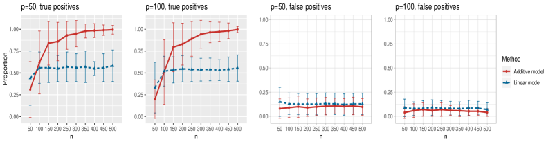
Figure 1: The proportion of the relevant covariates (i.e., the treatment effect-modifiers) correctly selected (the “true positives”; left two panels), and the irrelevant covariates (i.e., the noise covariates) incorrectly selected (the “false positives”; right two panels), respectively (and $\pm 1$ standard deviation), as the training sample size $n$ varies from $50$ to $500$, for each $p\in\{50,100\}$. Two methods were compared: 1) the proposed additive model (solid curves), and 2) the linear model (MC) approach (dashed curves).

Figure 1 summarizes the results of the treatment effect-modifier selection performance with respect to the true/false positive rates (the left/right two panels, respectively), comparing the proposed additive regression to the linear regression approach, which are reported as the averages (and $\pm 1$ standard deviations) across the $200$ simulation replications. Figure 1 illustrates that, for the both $p=50$ and $p=100$ cases, the proportion of the correctly selecting treatment effect-modifiers (i.e., the “true positive”; the left two panels) of the additive regression method (the red solid curves) tends to $1$, with $n$ increasing from $n=50$ to $n=500$, while the proportion of incorrectly selecting treatment effect-modifiers (i.e., the “false positive”; the right two panels) tends to be bounded above by a small number. On the other hand, the proportion of correctly selecting treatment effect-modifiers for the linear regression method (the blue dotted curves) tends to be only around $0.5$ for both choices of $p$. The linear regression method selects only one treatment effect-modifier $X_{1}$ which has a linear interaction effect with $A$, while generally not selecting the other treatment effect-modifier $X_{2}$, i.e., the one that has the nonlinear (cosine) interaction effect (see (21) for the setting) with $A$.

4.2 Individualized treatment rule estimation performance

In this subsection, we assess the optimal ITR estimation performance of the proposed method based on simulations. We generate a vector of covariates $\bm{X}=(X_{1},\ldots,X_{p})^{\top}\in\mathbb{R}^{p}$ based on a multivariate normal distribution with each component having the marginal distribution $\mathcal{N}(0,(\pi/2)^{2})$ with the correlation between the components $\mbox{corr}(X_{j},X_{k})=0.1^{|j-k|}$. In this illustration, we consider $p=50$. Responses were generated, for 1) “nonlinear” $A$-by-$\bm{X}$ interactions:

$$Y=\ \delta\sum_{j=1}^{5}\sin(X_{j})\ +\ 2(A-1.5)\big{\{}\cos(X_{1})-\cos(X_{2})+\xi\sin(X_{1}X_{2})\big{\}}\ +\ \epsilon\quad A\in\{1,2\},$$ (23)

and for 2) “linear” $A$-by-$\bm{X}$ interactions:

$$Y=\ \delta\sum_{j=1}^{5}\sin(X_{j})\ +\ (A-1.5)\big{\{}X_{1}-X_{2}+\xi X_{1}X_{2}\big{\}}\ +\ \epsilon\quad A\in\{1,2\},$$ (24)

where the treatment variable $A\in\{1,2\}$ is generated independently from the covariates $\bm{X}$ and the error term $\epsilon\sim\mathcal{N}(0,0.5^{2})$, such that $\mbox{Pr}(A=1)=\mbox{Pr}(A=2)=1/2$. Models (23) and (24) are indexed by a pair $\{\delta,\xi\}$. The parameter $\delta\in\{1,2\}$ controls the proportion of the variance of the response $Y$ attributable to the $\bm{X}$ “main” effect: $\delta=1$ corresponds to a moderate $\bm{X}$ main effect contribution; $\delta=2$ corresponds to a large $\bm{X}$ main effect contribution. Estimation of the interaction effect becomes more difficult with a larger $\delta$. The parameter $\xi\in\{0,1\}$ determines whether the $A$-by-$\bm{X}$ interaction effect term has an exact additive regression structure $(\xi=0)$ or whether it deviates from an additive structure $(\xi=1)$. In the case of $\xi=0$, the proposed model (1) is correctly specified, whereas, for the case of $\xi=1$, model (1) is misspecified. For each scenario, we consider the following four approaches to estimating the optimal ITR $\mathcal{D}^{opt}$ in (20).

1. The proposed additive regression approach (6), estimated via Algorithm 1. The dimension of the basis function $\bm{\Psi}_{j}$ in (10) is taken to be $d_{j}=6$ $(j=1,\ldots,p)$. Given estimates $\{\hat{g}_{j}^{\ast}\}$, the estimate of $\mathcal{D}^{opt}$ in (20) is $\hat{\mathcal{D}}^{opt}(\bm{X})=\operatorname*{arg\,max}_{a\in\{1,\ldots,L\}}\sum_{j=1}^{p}\hat{g}_{j,a}^{\ast}(X_{j})$.

2. The linear regression (MC) approach (22) of Tian and others (2014), implemented through the R-package glmnet, with the sparsity tuning parameter $\lambda$ selected by minimizing a 10-fold cross-validated prediction error. Given an estimate $\hat{\bm{\beta}}^{\ast}=(\hat{\beta}_{1}^{\ast},\ldots,\hat{\beta}_{p}^{\ast})^{\top}$, the corresponding estimate of $\mathcal{D}^{opt}$ in (20) is $\hat{\mathcal{D}}^{opt}(\bm{X})=\operatorname*{arg\,max}_{a\in\{1,\ldots,L\}}\sum_{j=1}^{p}(a-1.5)X_{j}\hat{\beta}_{j}^{\ast}$.

3. The outcome weighted learning (OWL) method (Zhao and others, 2012) based on a Gaussian radial kernel, implemented in the R-package DTRlearn, with a set of feature transformed (FT) covariates $\{\hat{g}_{j,1}^{\ast}(X_{j}),j=1,\ldots,p\}$ used as an input to the OWL method, in which the functions $\hat{g}_{j,1}^{\ast}(\cdot)$ $(j=1,\ldots,p)$ are obtained from the approach in 1. To improve the efficiency of the OWL, we employ the augmented OWL approach of Liu and others (2018). The inverse bandwidth parameter $\sigma_{n}^{2}$ and the tuning parameter $\kappa$ in Zhao and others (2012) are chosen from the grid of $(0.01,0.02,0.04,\ldots,0.64,1.28)$ and that of $(0.25,0.5,1,2,4)$ (the default setting of DTRlearn), respectively, based on a $5$ fold cross-validation.

4. The same (OWL) approach as in 3 but based on the original features $\{X_{j},j=1,\ldots,p\}$.

For each simulation run, we estimate $\mathcal{D}^{opt}$ from each of the four methods based on a training set (of size $n\in\{250,500\}$), and for evaluation of these methods, we compute the value $V(\hat{\mathcal{D}}^{opt})$ in (19) for each estimate $\hat{\mathcal{D}}^{opt}$, using a Monte Carlo approximation based on a random sample of size $10^{3}$. Since we know the true data generating model in simulation studies, the optimal $\mathcal{D}^{opt}$ can be determined for each simulation run. Given each estimate $\hat{\mathcal{D}}^{opt}$ of $\mathcal{D}^{opt}$, we report $V(\hat{\mathcal{D}}^{opt})-V(\mathcal{D}^{opt})$, as the performance measure of $\hat{\mathcal{D}}^{opt}$. A larger value (i.e., a smaller difference from the optimal value) of the measure indicates better performance.

.

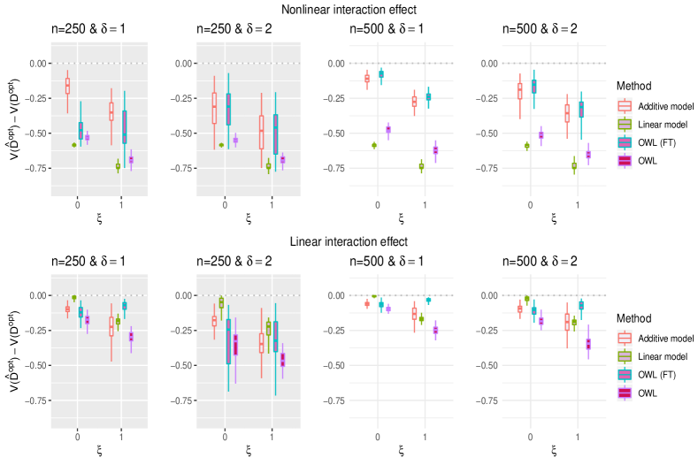
Figure 2: Boxplots obtained from $100$ Monte Carlo simulations comparing 4 approaches to estimating $\mathcal{D}^{opt}$, given each scenario indexed by $\xi\in\{0,1\}$, $\delta\in\{1,2\}$ and $n\in\{250,500\}$, for the nonlinear $A$-by-$\bm{X}$ interaction effect case in the top panels, and the linear $A$-by-$\bm{X}$ interaction effect case in the bottom panels. The dotted horizontal line represents the optimal value corresponding to $\mathcal{D}^{opt}$.

In Figure 2, we present the boxplots, obtained from $100$ simulation runs, of the normalized values $V(\hat{\mathcal{D}}^{opt})$ (normalized by the optimal values $V(\mathcal{D}^{opt})$) of the decision rules $\hat{\mathcal{D}}^{opt}$ estimated from the four approaches, for each combination of $n\in\{250,500\}$, $\xi\in\{0,1\}$ (corresponding to correctly-specified or mis-specified additive interaction effect models, respectively) and $\delta\in\{1,2\}$ (corresponding to moderate or large main effects, respectively), for the nonlinear and the linear $A$-by-$\bm{X}$ interaction effect scenarios, in the top and bottom panels, respectively. The proposed additive regression clearly outperforms the OWL (without feature transformation) method in all scenarios (both the top and bottom panels), and the linear regression approach in all of the nonlinear $A$-by-$\bm{X}$ interaction effect scenarios (the top panels). For the linear $A$-by-$\bm{X}$ interaction effect scenarios (the bottom panels), when $\xi=0$ (i.e., when the linear interaction model is correctly specified), the linear regression outperforms the additive regression, but only slightly, whereas if the underlying model deviates from the exact linear structure (i.e., $\xi=1$ in model (24)) and $n=500$, the more flexible additive regression tends to outperform the linear model. This suggests that, in the absence of prior knowledge about the form of the interaction effect, for optimizing ITRs, employing the proposed additive regression is more suitable than the linear regression. Comparing the two OWL methods (OWL (FT) and OWL), Figure 2 illustrates that the feature transformation provides a considerable benefit in their performance. This suggests the utility of the estimated component functions $\{\hat{g}_{j}^{\ast},j=1,\ldots,p\}$ of the proposed additive model as a potential feature transformation and selection tool for a machine learning algorithm for optimizing ITRs. Comparing the cases with $\delta=2$ to those with $\delta=1$, the increased magnitude of the main effect generally dampens the performance of all approaches, as the “noise” variability in the data generation model increases.

5 Application to data from a depression clinical trial

In this section, we illustrate the utility of the proposed additive regression for estimating treatment effect-modification and optimizing individualized treatment rules, using data from a depression clinical trial study, comparing an antidepressant and placebo for treating major depressive disorder (Trivedi and others, 2016). The goal of the study is to identify baseline characteristics that are associated with differential response to the antidepressant versus placebo and to use those characteristics to guide treatment decisions when a patient presents for treatment.

Study participants (a total of $n=166$ participants) were randomized to either placebo ($A=1$; $n_{1}=88$) or an antidepressant (sertraline) ($A=2$; $n_{2}=78$). Subjects were monitored for 8 weeks after initiation of treatment, and the primary endpoint of interest was the Hamilton Rating Scale for Depression (HRSD) score at week 8. The outcome $Y$ was taken to be the improvement in symptoms severity from baseline to week $8$, taken as the difference, i.e., we take: week 0 HRSD score - week 8 HRSD score. (Larger values of the outcome $Y$ are considered desirable.) The study collected baseline patient clinical data, prior to treatment assignment. These pretreatment clinical data $\bm{X}=(X_{1},X_{2},\ldots,X_{13})^{\top}\in\mathbb{R}^{13}$ include: $X_{1}=$ Age at evaluation; $X_{2}=$ Severity of depressive symptoms measured by the HRSD at baseline; $X_{3}=$ Logarithm of duration (in month) of the current major depressive episode; and $X_{4}=$ Age of onset of the first major depressive episode. In addition to these standard clinical assessments, patients underwent neuropsychiatric testing at baseline to assess psychomotor slowing, working memory, reaction time (RT) and cognitive control (e.g., post-error recovery), as these behavioral characteristics are believed to correspond to biological phenotypes related to response to antidepressants (Petkova and others, 2017) and are considered as potential modifiers of the treatment effect. These neuropsychiatric baseline test measures include: $X_{5}=$ (A not B) RT-negative; $X_{6}=$ (A not B) RT-non-negative; $X_{7}=$(A not B) RT-all; $X_{8}=$ (A not B) RT-total correct; $X_{9}=$ Median choice RT; $X_{10}=$ Word fluency; $X_{11}=$ Flanker accuracy; $X_{12}=$ Flanker RT; $X_{13}=$ Post conflict adjustment.

The proposed approach (6) to estimating the $A$-by-$\bm{X}$ interaction effect part $\sum_{j=1}^{p}g_{j,A}^{\ast}(X_{j})$ of model (1), estimated via Algorithm 1, simultaneously selected $3$ pretreatment covariates as treatment effect-modifiers: $X_{1}$ (“Age at evaluation”), $X_{10}$ (“Word fluency test”) and $X_{11}$ (“Flanker accuracy test”). Figure 3 illustrates the estimated non-zero component functions $\{\hat{g}_{j}^{\ast}\neq 0,j=1,\ldots,13\}$ (i.e., the component functions corresponding to the selected covariates $X_{1}$, $X_{10}$ and $X_{11}$) and the associated partial residuals. The linear regression approach (22) to estimating the $A$-by-$\bm{X}$ interactions selected a single covariate, $X_{11}$, as a treatment effect-modifier.

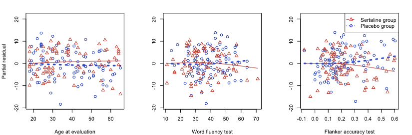
Figure 3: Scatterplots of partial residuals vs. the covariates associated with estimated non-zero component functions $\{\hat{g}_{j}^{\ast}\neq 0\}$ for placebo (blue circles) and the active drug (red triangles) treated participants. For each panel, the blue dashed curve represents $\hat{g}_{j,1}^{\ast}(\cdot)$, corresponding to the placebo ($a=1$), and the red solid curve represents $\hat{g}_{j,2}^{\ast}(\cdot)$, corresponding to the active drug ($a=2$).

To evaluate the performance of the ITRs ($\hat{\mathcal{D}}^{opt}$) obtained from the four different approaches described in Section 4.2, we randomly split the data into a training set and a testing set (of size $\tilde{n})$ using a ratio of $5$ to $1$, replicated $500$ times, each time computing an ITR $\hat{\mathcal{D}}^{opt}$ based on the training set, then estimating its value $V(\hat{\mathcal{D}}^{opt})$ in (19) by an inverse probability weighted estimator (Murphy, 2005): $\hat{V}(\hat{\mathcal{D}}^{opt})=\sum_{i=1}^{\tilde{n}}Y_{i}I_{(A_{i}=\hat{\mathcal{D}}^{opt}(\bm{X}_{i}))}/\sum_{i=1}^{\tilde{n}}I_{(A_{i}=\hat{\mathcal{D}}^{opt}(\bm{X}_{i}))}$, computed based on the testing set of size $\tilde{n}$. For comparison, we also include two naïve rules: treating all patients with placebo (“All PBO”) and treating all patients with the active drug (“All DRUG”), each regardless of the individual patient’s characteristics $\bm{X}$. The resulting boxplots obtained from the $500$ random splits are illustrated in Figure 4. A larger value of the measure indicates better performance.

.

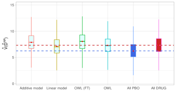
Figure 4: Boxplots of the estimated values of the treatment rules $\hat{\mathcal{D}}^{opt}$ estimated from $6$ approaches, obtained from $500$ randomly split testing sets. Higher values are preferred.

The results in Figure 4 demonstrate that the proposed additive regression approach, which allows nonlinear flexibility in developing ITRs, tends to outperform the linear regression approach, in terms of the estimated value. The additive regression approach also shows some superiority over the method OWL (without feature transformation). In comparison to the OWL methods, the proposed additive regression, in addition to its superior computational efficiency, provides a means of simultaneously selecting treatment effect-modifiers and allows a visualization for the heterogeneous effects attributable to each estimated treatment effect-modifier as in Figure 3, which is an appealing feature in practice. Moreover, the estimated component functions $\{\hat{g}_{j}^{\ast},j=1,\ldots,p\}$ of the proposed regression provide an effective means of performing feature transformation for $\{X_{j},j=1,\ldots,p\}$. As in Section 4.2, the feature transformed OWL approach appears to have a considerable improvement over the OWL that bases on the original untransformed covariates.

6 Discussion

In this paper, we have developed a sparse additive model, via a structural constraint, specifically geared to identify and model treatment effect-modifiers. The approach utilizes an efficient back-fitting algorithm for model estimation and variable selection. The proposed sparse additive model for treatment effect-modification extends existing linear model-based regression methods by providing nonlinear flexibility to modeling treatment-by-covariate interactions. Encouraged by our simulation results and the application, future work will investigate the asymptotic properties related to treatment effect-modifier selection and estimation consistency, in addition to developing hypothesis testing procedures for treatment-by-covariates interaction effects.

Modern advances in biotechnology, using measures of brain structure and function obtained from neuroimaging modalities (e.g., MRI, fMRI and EEG), show the promise of discovering potential biomarkers for heterogeneous treatment effects. These high dimensional data modalities are often in the form of curves or images and can be viewed as functional data (e.g., Ramsay and Silverman, 1997). Future work will also extend the additive model approach to the context of functional additive regression (e.g., Fan and others, 2015, 2014). The goal of these extensions will be to handle a large number of functional-valued covariates while achieving simultaneous variable selection, which will extend current functional linear model-based methods for precision medicine (McKeague and Qian, 2014; Ciarleglio and others, 2015, 2018) to a more flexible functional regression setting.

7 Software

R-package samTEMsel (Sparse Additive Models for Treatment Effect-Modifier Selection) contains R-codes to perform the methods proposed in the article, and is publicly available on GitHub (syhyunpark/samTEMsel).

8 Supplementary Materials

The Supplementary Materials including the proof of Theorem 3.1 and the R-codes and the dataset used in this article are available online at http://biostatistics.oxfordjournals.org.

Supplementary Materials

Proof of Theorem 1

Proof 8.1.

The squared error criterion on the right-hand side of (2.6) of the main manuscript is

$$\mathbb{E}\bigg{[}\big{\{}Y-\sum_{j=1}^{p}g_{j,A}(X_{j})\big{\}}^{2}\bigg{]}\propto \ \mathbb{E}\bigg{[}Y\sum_{j=1}^{p}g_{j,A}(X_{j})-\big{\{}\sum_{j=1}^{p}g_{j,A}(X_{j})\big{\}}^{2}/2\bigg{]}\quad\mbox{(with respect to }\{g_{j}\})$$ (25)

$$= \ \mathbb{E}\bigg{[}\big{\{}\mu^{\ast}(\bm{X})+\sum_{j=1}^{p}g_{j,A}^{\ast}(X_{j})\big{\}}\sum_{j=1}^{p}g_{j,A}(X_{j})-\big{\{}\sum_{j=1}^{p}g_{j,A}(X_{j})\big{\}}^{2}/2\bigg{]}$$

$$= \ \mathbb{E}\bigg{[}\mu^{\ast}(\bm{X})\sum_{j=1}^{p}g_{j,A}(X_{j})\bigg{]}+\mathbb{E}\bigg{[}\big{\{}\sum_{j=1}^{p}g_{j,A}^{\ast}(X_{j})\big{\}}\big{\{}\sum_{j=1}^{p}g_{j,A}(X_{j})\big{\}}-\big{\{}\sum_{j=1}^{p}g_{j,A}(X_{j})\big{\}}^{2}/2\bigg{]}$$

$$= \ \mathbb{E}\bigg{[}\big{\{}\sum_{j=1}^{p}g_{j,A}^{\ast}(X_{j})\big{\}}\big{\{}\sum_{j=1}^{p}g_{j,A}(X_{j})\big{\}}-\big{\{}\sum_{j=1}^{p}g_{j,A}(X_{j})\big{\}}^{2}/2\bigg{]},$$

where the last equality follows from the constraint $\mathbb{E}[g_{j,A}(X_{j})|X_{j}]=0$ $(j=1,\ldots,p)$ in (2.6) of the main manuscript imposed on $\{g_{j}\}$, and by noting $\mathbb{E}\big{[}\mu^{\ast}(\bm{X})\sum_{j=1}^{p}g_{j,A}\big{(}X_{j}\big{)}\big{]}=\mathbb{E}\big{[}\mathbb{E}\big{[}\mu^{\ast}(\bm{X})\sum_{j=1}^{p}g_{j,A}(X_{j})|\bm{X}\big{]}\big{]}=\mathbb{E}\big{[}\mu^{\ast}(\bm{X})\sum_{j=1}^{p}\mathbb{E}\big{[}g_{j,A}(X_{j})|X_{j}\big{]}\big{]}=0$. From (25), the squared error criterion in (2.6) of the main manuscript can be expressed as:

$$\underset{\{g_{j}\in\mathcal{H}_{j}\}}{\text{argmin}}\ \mathbb{E}\bigg{[}\big{(}Y-\sum_{j=1}^{p}g_{j,A}\big{(}X_{j}\big{)}\big{)}^{2}\bigg{]}\ =\ \underset{\{g_{j}\in\mathcal{H}_{j}\}}{\text{argmin}}\ \mathbb{E}\bigg{[}\big{(}\sum_{j=1}^{p}g_{j,A}^{\ast}\big{(}X_{j}\big{)}-\sum_{j=1}^{p}g_{j,A}\big{(}X_{j}\big{)}\big{)}^{2}\bigg{]}.$$ (26)

In the following, we closely follow the proof of Theorem 1 in Ravikumar and others (2009). The constrained objective function in (2.6) of the main manuscript can be rewritten in Lagrangian form as:

$$Q(\{g_{j}\};\lambda):=\mathbb{E}\bigg{[}\big{(}\sum_{j=1}^{p}g_{j,A}^{\ast}(X_{j})-\sum_{j=1}^{p}g_{j,A}(X_{j})\big{)}^{2}\bigg{]}+\lambda\sum_{j=1}^{p}\lVert g_{j}\rVert$$ (27)

For the notational simplicity, let us write $g_{j}=g_{j,A}(X_{j})$. For each $j$, consider the minimization of (27) with respect to the component function $g_{j}\in\mathcal{H}_{j}$, holding the other component functions $\{g_{j^{\prime}},j^{\prime}\neq j\}$ fixed. The stationary condition is obtained by setting its Fréchet derivative to 0. Denote by $\partial_{j}Q(\{g_{j}\};\lambda;\eta_{j})$ the directional derivative with respect to $g_{j}$ $(j=1,\ldots,p)$ in the direction, say, $\eta_{j}\in\mathcal{H}_{j}$. Then, the stationary point of the Lagrangian (27) can be formulated as:

$$\partial_{j}Q(\{g_{j}\};\lambda;\eta_{j})=2\mathbb{E}\left[(g_{j}-\tilde{R}_{j}+\lambda\nu_{j})\eta_{j}\right]=0,$$ (28)

where

$$\tilde{R}_{j}:=\sum_{j=1}^{p}g_{j,A}^{\ast}(X_{j})-\sum_{j^{\prime}\neq j}g_{j^{\prime},A}(X_{j})$$ (29)

is the partial residual for $g_{j}$, and $\nu_{j}$ is an element of the subgradient $\partial\lVert g_{j}\rVert$, which satisfies $\nu_{j}=g_{j}/\lVert g_{j}\rVert$ if $\lVert g_{j}\rVert\neq 0$, and $\nu_{j}\in\{s\in\mathcal{H}_{j}\mid\lVert s\rVert\leq 1\}$, otherwise. Using iterated expectations conditional on $X_{j}$ and $A$, (28) can be rewritten as

$$2\mathbb{E}\left[\left(g_{j}-\mathbb{E}\left[\tilde{R}_{j}|X_{j},A\right]+\lambda\nu_{j}\right)\eta_{j}\right]=0.$$ (30)

Since $g_{j}-\mathbb{E}\left[\tilde{R}_{j}|X_{j},A\right]+\lambda\nu_{j}\in\mathcal{H}_{j}$, we can evaluate (28) (i.e., (30)) in the direction: $\eta_{j}=g_{j}-\mathbb{E}\left[\tilde{R}_{j}|X_{j},A\right]+\lambda\nu_{j}$, implying $\mathbb{E}\left[\left(g_{j}-\mathbb{E}\left[\tilde{R}_{j}|X_{j},A\right]+\lambda\nu_{j}\right)^{2}\right]=0.$ This implies:

$$g_{j}+\lambda\nu_{j}=\mathbb{E}\left[\tilde{R}_{j}|X_{j},A\right]\quad\mbox{(almost surely).}$$ (31)

Let $f_{j}$ denote the right-hand side of (31), i.e., $f_{j}(=f_{j,A}(X_{j})):=\mathbb{E}\left[\tilde{R}_{j}|X_{j},A\right]$. If $\lVert g_{j}\rVert\neq 0$, then $\nu_{j}=g_{j}/\lVert g_{j}\rVert$. Therefore, by (31), we have $\lVert f_{j}\rVert=\lVert g_{j}+\lambda g_{j}/\lVert g_{j}\rVert\rVert=\lVert g_{j}\rVert+\lambda\geq\lambda$. On the other hand, if $\lVert g_{j}\rVert=0$, then $g_{j}=0$ (almost surely) and $\lVert\nu_{j}\rVert\leq 1$ which, together with condition (31), implies that $\lVert f_{j}\rVert\leq\lambda$. This gives us the equivalence between $\lVert f_{j}\rVert\leq\lambda$ and the statement $g_{j}=0$ (almost surely). Therefore, condition (31) leads to the following expression:

$$\left(1+\lambda/\lVert g_{j}\rVert\right)g_{j}=f_{j}\quad\mbox{(almost surely)}$$

if $\lVert f_{j}\rVert>\lambda$; otherwise, and $g_{j}=0$ (almost surely). This gives the soft thresholding update rule for $g_{j}$.

The underlying model (2.1) of the main manuscript indicates that $\sum_{j=1}^{p}g_{j,A}^{\ast}(X_{j})=\mathbb{E}[Y|X,A]-\mu^{\ast}(\bm{X})$. Thus, (29) can be equivalently written as: $\tilde{R}_{j}=\mathbb{E}[Y|X,A]-\mu^{\ast}(\bm{X})-\sum_{j^{\prime}\neq j}g_{j^{\prime},A}(X_{j^{\prime}}).$ Therefore, the function $f_{j,A}(X_{j})=\mathbb{E}\left[\tilde{R}_{j}|X_{j},A\right]$ can be written by:

$$f_{j,A}(X_{j}) =\mathbb{E}\big{[}\mathbb{E}[Y|X,A]-\mu^{\ast}(\bm{X})-\sum_{j^{\prime}\neq j}g_{j^{\prime},A}(X_{j^{\prime}})\mid X_{j},A\big{]}$$

$$=\mathbb{E}\big{[}\mathbb{E}[Y|X,A]-\sum_{j^{\prime}\neq j}g_{j^{\prime},A}(X_{j^{\prime}})|X_{j},A\big{]}-\mathbb{E}\big{[}\mu^{\ast}(\bm{X})|X_{j},A\big{]}$$

$$=\mathbb{E}\big{[}Y-\sum_{j^{\prime}\neq j}g_{j^{\prime},A}(X_{j^{\prime}})|X_{j},A\big{]}-\mathbb{E}\big{[}\mu^{\ast}(\bm{X})|X_{j}\big{]}$$

$$=\mathbb{E}\big{[}Y-\sum_{j^{\prime}\neq j}g_{j^{\prime},A}(X_{j^{\prime}})|X_{j},A\big{]}-\mathbb{E}\big{[}\mu^{\ast}(\bm{X})+\sum_{j=1}^{p}g_{j,A}^{\ast}\big{(}X_{j}\big{)}|X_{j}\big{]}$$

$$=\mathbb{E}\big{[}Y-\sum_{j^{\prime}\neq j}g_{j^{\prime},A}(X_{j^{\prime}})|X_{j},A\big{]}-\mathbb{E}\big{[}Y|X_{j}\big{]}$$

$$=\mathbb{E}\big{[}Y-\sum_{j^{\prime}\neq j}g_{j^{\prime},A}(X_{j^{\prime}})|X_{j},A\big{]}-\mathbb{E}\big{[}Y-\sum_{j^{\prime}\neq j}g_{j^{\prime},A}(X_{j^{\prime}})|X_{j}\big{]}$$

$$=\mathbb{E}\big{[}R_{j}|X_{j},A\big{]}-\mathbb{E}\big{[}R_{j}|X_{j}\big{]},$$

where the fourth equality follows from the identifiability constraint (2.2) of the underlying model (2.1) of the main manuscript, and the sixth equality follows from the optimization constraint $\mathbb{E}[g_{j,A}(X_{j})|X_{j}]=0$ $(j=1,\ldots,p)$ in (2.6) of the main manuscript imposed on $\{g_{j}\}$; this gives the desired expression (3.8) of the main manuscript.

References

- Ciarleglio and others (2015) Ciarleglio, A., Petkova, E., Ogden, R. T. and Tarpey, Thaddeus. (2015). Treatment decisions based on scalar and functional baseline covariatesecisions based on scalar and functional baseline covariates. Biometrics 71(4), 884–894.
- Ciarleglio and others (2018) Ciarleglio, A., Petkova, E., Ogden, R. T. and Tarpey, Thaddeus. (2018). Constructing treatment decision rules based on scalar and functional predictors when moderators of treatment effect are unknown. Journal of Royal Statistical Society: Series C 67, 1331–1356.
- Fan and others (2014) Fan, Y., Foutz, N., James, G. M. and Jank, W. (2014). Functional response additive model estimation with online virtual stock markets. The Annals of Applied Statistics 8, 2435–2460.
- Fan and others (2015) Fan, Y., James, G. M. and Radchanko, P. (2015). Functional additive regression. The Annals of Statistics 43, 2296–2325.
- Hastie and Tibshirani (1999) Hastie, T. and Tibshirani, R. (1999). Generalized Additive Models. Chapman & Hall Ltd.
- Jeng and others (2018) Jeng, X., Lu, W. and Peng, H. (2018). High-dimensional inference for personalized treatment decision. Electronic Journal of Statistics 12, 2074–2089.
- Kang and others (2014) Kang, C., Janes, H. and Huang, Y. (2014). Combining biomarkers to optimize patient treatment recommendations. Biometrics 70, 696–707.
- Kuhn and Johnson (2019) Kuhn, Max and Johnson, Kjell. (2019). Feature Engineering and Selection: A Practical Approach for Predictive Models. Chapman and Hall/CRC.
- Laber and Zhao (2015) Laber, E. B. and Zhao, Y. (2015). Tree-based methods for individualized treatment regimes. Biometrika 102, 501–514.
- Liu and others (2018) Liu, Y., Wang, Y., Kosorok, M. R., Zhao, Y. and Zeng, D. (2018). Augmented outcome‐weighted learning for estimating optimal dynamic treatment regimens. Statistics in Medicine 37, 3776–3788.
- Lu and others (2011) Lu, W., Zhang, H. and Zeng, D. (2011). Variable selection for optimal treatment decision. Statistical Methods in Medical Research 22, 493–504.
- McKeague and Qian (2014) McKeague, I. and Qian, M. (2014). Estimation of treatment policies based on functional predictors. Statistica Sinica 24, 1461–1485.
- Murata and Amari (1994) Murata, N. and Amari, S. (1994). Network Information Criterion- Determining the number of hidden units for an artificial neural network model. IEEE Transactions on Neural Networks 5(6), 865–872.
- Murphy (2003) Murphy, S. A. (2003, May). Optimal dynamic treatment regimes. Journal of the Royal Statistical Society: Series B (Statistical Methodology) 65, 331–355.
- Murphy (2005) Murphy, S. A. (2005). A generalization error for q-learning. Journal of Machine Learning 6, 1073–1097.
- Petkova and others (2017) Petkova, E., Ogden, R.T., Tarpey, T., Ciarleglio, A., Jiang, B., Su, Z., Carmody, T., Adams, P., Kraemer, H., Grannemann, B., Oquendo, M., Parsey, R., Weissman, M., McGrath, P., Fava, M. and others. (2017). Statistical analysis plan for stage 1 embarc (establishing moderators and biosignatures of antidepressant response for clinical care) study. Contemporary Clinical Trials Communications 6, 22–30.
- Ramsay and Silverman (1997) Ramsay, J. O. and Silverman, B. W. (1997). Functional Data Analysis. New York: Springer.
- Ravikumar and others (2009) Ravikumar, P., Lafferty, J., Liu, H. and Wasserman, L. (2009). Sparse additive models. Journal of Royal Statistical Society: Series B 71, 1009–1030.
- Royston and Sauerbrei (2008) Royston, P. and Sauerbrei, W. (2008). Interactions between treatment and continuous covariates: A step toward individualizing therapy. Journal of Clinical Oncology 26(9), 1397–1399.
- Shi and others (2016) Shi, C., Song, R. and Lu, W. (2016). Robust learning for optimal treatment decision with np-dimensionality. Electronic Journal of Statistics 10, 2894–2921.
- Song and others (2015) Song, R., Kosorok, M., Zeng, D., Zhao, Y., Laber, E. B. and Yuan, M. (2015). On sparse representation for optimal individualized treatment selection with penalized outcome weighted learning. Stat 4, 59–68.
- Tian and others (2014) Tian, L., Alizadeh, A., Gentles, A. and Tibshrani, R. (2014). A simple method for estimating interactions between a treatment and a large number of covariates. Journal of the American Statistical Association 109(508), 1517–1532.
- Trivedi and others (2016) Trivedi, M., McGrath, P., Fava, M., Parsey, R., Kurian, B., Phillips, M., Pquendo, M., Bruder, G., Pizzagalli, D., Toups, M., Cooper, C., Adams, P., Weyandt, S., Morris, D., Grannemann, B., Ogden, R., Buckner, R., McInnis, M., Kraemer, H., Petkova, E., Carmody, T. and others. (2016). Establishing moderators and biosignatures of antidepressant response in clinical care (embarc): Rationale and design. Journal of Psychiatric Research 78, 11–23.
- Tseng (2001) Tseng, P. (2001). Convergence of block coordinate descent method for nondifferentiable maximation. Journal of Optimization Theory and Applications 109, 474–494.
- Zhang and others (2012) Zhang, B., Tsiatis, A. A., Davidian, M., Zhang, M. and Laber, E. (2012). Estimating optimal treatment regimes from classification perspective. Stat 1, 103–114.
- Zhao and others (2019) Zhao, Y., Laber, E., Ning, Y., Saha, S. and Sands, B. (2019). Efficient augmentation and relaxation learning for individualized treatment rules using observational data. Journal of Machine Learning Research 20, 1–23.
- Zhao and others (2012) Zhao, Y., Zeng, D., Rush, A. J. and Kosorok, M. R. (2012). Estimating individualized treatment rules using outcome weighted learning. Journal of the American Statistical Association 107, 1106–1118.
- Zhao and others (2015) Zhao, Y., Zheng, D., Laber, E. B. and Kosorok, M. R. (2015). New statistical learning methods for estimating optimal dynamic treatment regimes. Journal of the American Statistical Association 110, 583–598.