Neural Bipartite Matching
Abstract
Graph neural networks (GNNs) have found application for learning in the space of algorithms. However, the algorithms chosen by existing research (sorting, Breadth-First search, shortest path finding, etc.) usually align perfectly with a standard GNN architecture. This report describes how neural execution is applied to a complex algorithm, such as finding maximum bipartite matching by reducing it to a flow problem and using Ford-Fulkerson to find the maximum flow. This is achieved via neural execution based only on features generated from a single GNN. The evaluation shows strongly generalising results with the network achieving optimal matching almost 100% of the time.
1 Introduction
Many real-world problems can be formulated as graph problems – social relations, protein folding, web search, etc. Throughout the years graph algorithms for solving these tasks have been discovered. One such task is the problem of finding the maximum flow from a source to a sink in a graph whose edges have certain capacities . (Imagine material flowing source sink). Any flow must obey two important properties: the flow on each edge should not exceed the capacity, i.e. and for all nodes except source and sink flow should be preserved, i.e. . Algorithms for finding maximum flow have found applications in many areas, such as bipartite matching (attempted here), airline scheduling or image segmentation (Boykov & Funka-Lea, 2006).
The main topic of this work is evaluating whether graph neural networks (GNNs) are able to reason like a complex algorithm, specifically, whether they can be used for finding optimal bipartite matching using the Ford-Fulkerson (Ford & Fulkerson, 1956) algorithm for finding maximum flow. Performing the reasoning is achieved via neural execution, in a similar fashion to Veličković et al. (2020). GNNs have been both empirically (Veličković et al., 2020) and theoretically (Xu et al., 2020) shown to be applicable to algorithmic tasks on graphs, strongly generalising on inputs of sizes much larger than trained on. However, these algorithms rely on a locally contained and fixed dataflow which aligns perfectly with a standard GNN architecture, making them easy to model with GNNs (c.f. Xu et al., 2020).
Our contributions are three-fold: 1) We successfully show that GNNs are suitable for learning a complex algorithm, namely Ford-Fulkerson, which consists of several composable subroutines. To the best of our knowledge, this is the first time such an algorithm is neurally executed with GNNs. 2) We demonstrate that GNNs can learn to respect the invariants of a complex algorithm. 3) We devised an evaluation which not only separately takes into account the accuracy of the subroutines, but assesses the performance of the Ford-Fulkerson algorithm as a whole – an inconsistency even in one of the subroutines can invalidate the whole algorithm.
2 Background
2.1 Ford-Fulkerson
For presentational purposes consider a concise version of Ford-Fulkerson algorithm given in Cormen et al. (2009) which operates directly on the residual graph with residual capacities derived from the input flow graph. The source and sink of the network are and :
The algorithm above has three key subroutines the neural network has to learn – finding augmenting path, finding minimum (bottleneck) capacity on the path and augmenting the residual capacities along the path.
2.2 Algorithm Execution
Preliminary definitions
The GNN receives a sequence of graphs with the same structure (vertices edges), but different features representing the execution of an algorithm. Let the graph be . At each timestep , each node has node features and each edge has edge features . At each step of the algorithm node-level outputs are produced, which are later reused in .
Encode-process-decode
The execution of an algorithm proceeds by the encode process decode paradigm (Hamrick et al., 2018). For each algorithm , an encoder network produces the algorithm-specific inputs The result is then processed using the processor network , which is shared across all algorithms. The processor takes as input encoded inputs and edge features to produce latent features : Algorithm specific outputs are calculated by its corresponding decoder network . Termination of the algorithm is decided by a termination network, , specific for each algorithm. The probability of the termination of an algorithm is obtained by applying the logistic sigmoid activation to the outputs of . This is summarised as:
| (1) | ||||
| (2) | ||||
| (3) | ||||
| (4) |
where . The execution of the algorithm proceeds while and . The algorithm is always terminated in steps.
Supervising algorithm execution
The aim for every algorithm is to learn to replicate the actual execution as close as possible. To achieve this, the supervision signal is driven by the actual algorithm outputs at every step .
For more details, please refer to Veličković et al. (2020).
3 Neurally Executing Ford-Fulkerson
On a high-level, execution proceeds as in Figure 1. The neural network computes an augmenting path from an input residual graph. Then, given the path, the bottleneck on it is found and the capacities on the path are changed according to Algorithm 1. The resulting new residual graph is reused as input to the next step and this process repeats until termination of the algorithm.
Finding Augmenting Path
One of the key challenges to the task of finding an augmenting path was deciding how the supervision signal is generated. Supervising towards algorithms such as Breadth-First/Depth-First search turned out to bee too difficult to train, since the algorithm and the learner could choose a different augmenting path (in both cases valid), but the learner is ‘penalised’ for its decision.
The solution to this problem is presented above. Additional weights are attached to each edge (edges are in the format capacity/weight). Now, if we choose to find the shortest path111It is theoretically possible that two shortest paths exist, but in practice this rarely occurred., the bottom path (green) is preferred over the top one (red). This changes the task from finding an augmenting path to finding the shortest augmenting path, given the additional weights. Finding the shortest path with the Bellman-Ford algorithm (Bellman, 1958) can be achieved by learning to predict predecessors for each node (Veličković et al., 2020). The network needs to learn to ignore zero capacity edges.
Bottleneck Finding
After an augmenting path is found, the next step is to find the bottleneck capacity along this path. All edges not on the augmenting path are masked out (deterministically) and each edge is assigned a probability of being the bottleneck. Inspired by Yan et al. (2020), the probabilities were generated using a readout attention computed from the messages between edges produced by the GNN from the last Bellman-Ford timestep. We have found that a single Transformer encoder layer (Vaswani et al., 2017) followed by a fully-connected layer is sufficient for our task.
Augmenting Path Capacities
Assuming integer capacities222This does not make the problem less general. predicting the edge capacities after the augmentation is achieved using logistic regression over the possible new forward capacities. For each edge with capacity , based on the message generated for this edge by the GNN, we assign probabilities to each number of the range . Each forward-backward edge capacity pair keeps constant sum.
To provide unique supervision signal for the above two tasks, random walks of length 5 are generated, together with random integer edge capacities in the range [1; 10].
4 Evaluation through simulation
Simply evaluating each step separately may not provide sufficient insight on how well the algorithm is learnt – discrepancies in either subroutine can nullify the correctness of the algorithm. Here we present evaluation through simulation, which simulates the Ford-Fulkerson from Algorithm 1. Algorithm 2 summarises the simulation. Subroutine details and design decisions are discussed below.
Finding Augmenting Path and Termination
The main issue with this step is that it is not possible to distinguish whether a valid path does not exist or the network is unable to find it. A trivial heuristic is terminating the algorithm as soon as the network produces an invalid path containing a zero capacity edge. A slightly better approach is a thresholding heuristic – pre-defining a threshold hyperparameter and terminating the execution if the network is unable to find a path consecutive times. To add some non-determinism edge weights are randomised for every attempt.
A smarter approach would be to learn to predict which nodes are reachable in the residual network via edges with positive capacity using the Breadth-First Search (BFS) algorithm. Therefore we can decide to terminate the algorithm, by predicting whether the sink is reachable from the source. If predicted reachable, a possible path from the source to the sink is generated by predicting predecessors. This heuristic is less artificial than the previous one, but now we have no guarantee that the generated path is valid. However, the bottleneck finding subroutine can be used to detect the presence of a zero capacity edge.
Bottleneck Finding
Similar issue arises here: the network could predict a wrong edge as the bottleneck on the path, making the algorithm incorrect. If such an error occurs, the Ford-Fulkerson algorithm is terminated instantly. Under the bipartite matching setting this can only happen if the generated path is invalid. In such case if the network correctly predicts a zero capacity edge, the path-finding step is rerun again. A threshold is used to avoid endless loops.
Augmenting Path Capacities
The new predicted capacities are compared against the real ones and if they are different, the Ford-Fulkerson algorithm is terminated. This may appear as a too strict policy, but evaluation on the bipartite matching setting showed that the network learns to accurately perform this step.
Design Motivation
If any of the above subroutines is wrong the flow value produced will be lower than optimal. Incorrect path-finding will keep generating invalid paths. Badly learnt BFS, bottleneck finding or subtraction can cause premature termination. Additionally, a well-learnt bottleneck finding will allow for reruns to be generated, allowing the network to ‘correct’ itself, to some extent.
| Model | Accuracy | ||||
|---|---|---|---|---|---|
| scale | scale | scale | scale | ||
|
|||||
The code for neural execution and simulation can be found at https://anonymous.4open.science/r/0403d670-c7f0-43c8-ab90-aa2f010462e7/.
5 Evaluation
Dataset and training details
300 bipartite graphs are generated for training and 50 for validation. The probability of generating an edge between the two subsets was fixed at . Bipartite graph subset size was fixed at 8 as smaller sizes generated too few training examples. Both subset were chosen to have the same size, as the maximum flow (maximum matching) is dictated from the size of the smaller subset. All subroutines are learnt simultaneously. Adam optimiser (Kingma & Ba, 2015) was used for training (initial learning rate 0.0005, batch size 32) and early stopping with patience of 10 epochs on the last step predecessor validation accuracy was performed. Evaluating the ability to strongly generalise is performed on graphs with subset size 8, 16, 32 and 64 (50 graphs each). Standard deviations are obtained over 10 simulation runs.
Architectural details
Two types of GNNs are assessed for their ability to learn to execute the Ford-Fulkerson algorithm. These are Message-passing neural networks (MPNN) with maximisation aggregation rule (Gilmer et al., 2017) and Principal Neighbourhood Aggregation (PNA) (Corso et al., 2020) with the standard deviation (std) aggregator removed333The std aggregator for tasks with no input noise (such as algorithms) results in a model which overfits to the data.. Latent feature dimension was fixed to features. Inputs (capacities and weights) are given as 8-bit binary numbers. (Infinity is represented as the bit vector 111…1.) Similar to Yan et al. (2020), embedding vector is learnt for each bit position. For each -bit input , the input feature embedding is computed as .
Results and discussion
We report the accuracy of predicting a flow (matching) equal to the maximum one. Table 1 presents the accuracy at different scale. Under threshold based execution, only the path finding is performed neurally, since all generated paths will have edges with capacity 1.
An exciting observation is that even a threshold of 1, i.e. terminating Ford-Fulkerson as soon as an invalid path is generated, yields high accuracy – about 90% for the scale and more than 95% for other datasets. In other words, if a valid path exists, it is likely that the network will find it. A threshold of 3 gives a noticeable boost in the accuracy and a threshold of 5 turns out to be sufficient for an almost perfect execution. An MPNN processor, which uses BFS for termination and determines the bottleneck and edge capacities after augmentation performs better than threshold based termination when and is slightly worse than other choices of at scales and . A further ablation study (Appendix A) showed that the latter two subroutines have infinitesimal impact on the accuracy.
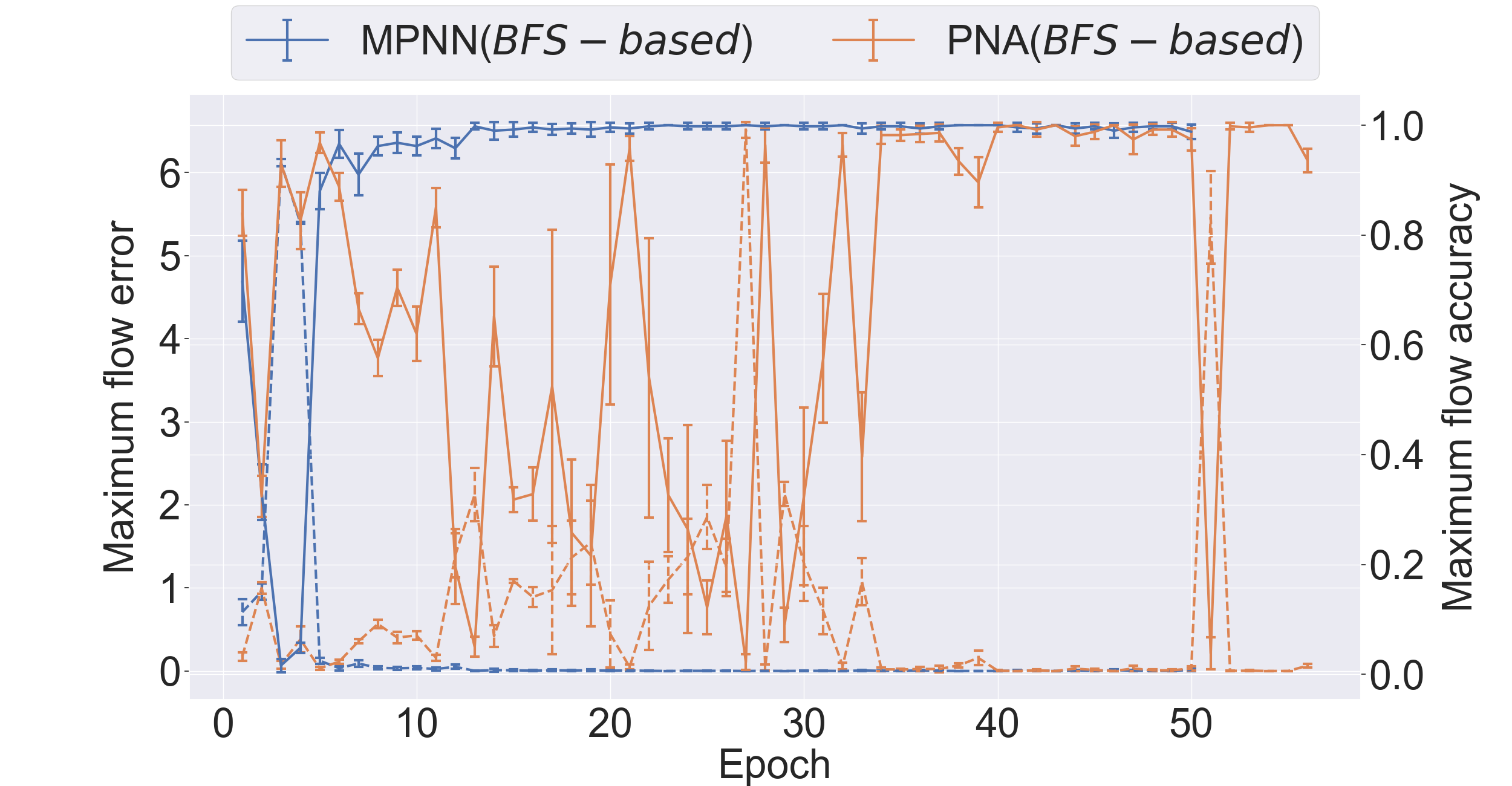
The best processor architecture was the PNA model, but the std aggregator had to be removed and the model required extra training data for the BFS task (see Appendix B). PNA also converged much more slowly than MPNN as can be seen from the flow accuracy per epoch for the 1 scale, given in Figure 2. Both networks exhibits some initial instability during the first epochs, but the MPNN was much more stable (convergence in 10 epochs, compared to 35). Both networks retained near 100% accuracy once they converged, with the only exception of epoch 51 for the PNA-based processor. Both models strongly generalise across all scales.
To further evaluate the strong generalisation ability, the two best-performing models were tested on bipartite graphs generated with different edge probability. 50 more test examples were generated for each of scale and . Both models performed equivalently and exhibited average accuracy higher than 99.73% across all test sets. Further details in Appendix C.
We have for the first time shown (near-)perfect strong generalisation for a complex algorithmic execution task. Based on this, we think that Algorithms and Deep Learning reinforce each other and we hope this paves to way to further related applications.
References
- Bellman (1958) Bellman, R. On a routing problem. Quarterly of Applied Mathematics, 16(1):87–90, 1958. ISSN 0033569X, 15524485. URL http://www.jstor.org/stable/43634538.
- Boykov & Funka-Lea (2006) Boykov, Y. and Funka-Lea, G. Graph cuts and efficient N-D image segmentation. Int. J. Comput. Vis., 70(2):109–131, 2006. doi: 10.1007/s11263-006-7934-5. URL https://doi.org/10.1007/s11263-006-7934-5.
- Cormen et al. (2009) Cormen, T. H., Leiserson, C. E., Rivest, R. L., and Stein, C. Introduction to Algorithms, 3rd Edition. MIT Press, 2009. ISBN 978-0-262-03384-8. URL http://mitpress.mit.edu/books/introduction-algorithms.
- Corso et al. (2020) Corso, G., Cavalleri, L., Beaini, D., Liò, P., and Veličković, P. Principal neighbourhood aggregation for graph nets. CoRR, abs/2004.05718, 2020. URL https://arxiv.org/abs/2004.05718.
- Ford & Fulkerson (1956) Ford, L. R. and Fulkerson, D. R. Maximal flow through a network. In Canadian Journal of Mathematics, pp. 399–404, 1956.
- Gilmer et al. (2017) Gilmer, J., Schoenholz, S. S., Riley, P. F., Vinyals, O., and Dahl, G. E. Neural message passing for quantum chemistry. In Proceedings of the 34th International Conference on Machine Learning, ICML 2017, Sydney, NSW, Australia, 6-11 August 2017, pp. 1263–1272, 2017. URL http://proceedings.mlr.press/v70/gilmer17a.html.
- Hamrick et al. (2018) Hamrick, J. B., Allen, K. R., Bapst, V., Zhu, T., McKee, K. R., Tenenbaum, J., and Battaglia, P. W. Relational inductive bias for physical construction in humans and machines. In Proceedings of the 40th Annual Meeting of the Cognitive Science Society, CogSci 2018, Madison, WI, USA, July 25-28, 2018, 2018. URL https://mindmodeling.org/cogsci2018/papers/0341/index.html.
- Kingma & Ba (2015) Kingma, D. P. and Ba, J. Adam: A method for stochastic optimization. In 3rd International Conference on Learning Representations, ICLR 2015, San Diego, CA, USA, May 7-9, 2015, Conference Track Proceedings, 2015. URL http://arxiv.org/abs/1412.6980.
- Vaswani et al. (2017) Vaswani, A., Shazeer, N., Parmar, N., Uszkoreit, J., Jones, L., Gomez, A. N., Kaiser, L., and Polosukhin, I. Attention is all you need. In Advances in Neural Information Processing Systems 30: Annual Conference on Neural Information Processing Systems 2017, 4-9 December 2017, Long Beach, CA, USA, pp. 5998–6008, 2017. URL http://papers.nips.cc/paper/7181-attention-is-all-you-need.
- Veličković et al. (2020) Veličković, P., Ying, R., Padovano, M., Hadsell, R., and Blundell, C. Neural execution of graph algorithms. In International Conference on Learning Representations, 2020. URL https://openreview.net/forum?id=SkgKO0EtvS.
- Xu et al. (2020) Xu, K., Li, J., Zhang, M., Du, S. S., Kawarabayashi, K., and Jegelka, S. What can neural networks reason about? In 8th International Conference on Learning Representations, ICLR 2020, Addis Ababa, Ethiopia, April 26-30, 2020, 2020. URL https://openreview.net/forum?id=rJxbJeHFPS.
- Yan et al. (2020) Yan, Y., Swersky, K., Koutra, D., Ranganathan, P., and Hashemi, M. Neural executon engines, 2020. URL https://openreview.net/forum?id=rJg7BA4YDr.
| Model | Accuracy | ||||||
|---|---|---|---|---|---|---|---|
| scale | scale | scale | scale | ||||
|
|||||||
|
|||||||
|
|||||||
|
|||||||
|
|||||||
|
|||||||
|
|||||||
|
|||||||
| Scale | Model | Accuracy | ||
|---|---|---|---|---|
|
||||
|
||||
Appendix A Subroutine impact
An ablation study of an MPNN based model (Table 2, top half) shows that using the network to perform the bottleneck finding and/or augmentation steps has minimal impact on the overall accuracy: In almost all cases mean accuracy remains within 1-2%. This is further supported by the following two observations. Setting an edge with capacity 0 to be a negative example and edge with 1 – positive, the average true negative rate for finding the bottleneck across all scales is . The average augmentation accuracy (correctness of capacities after augmentaiton) is . Given these observations and the fact that the accuracy has a standard deviation of 2.65%, the differences could be accredited to the BFS occasionally mispredicting the sink as unreachable on the last iteration of the Ford-Fulkerson algorithm.
Appendix B PNA is not highly suitable for the task of graph algorithm execution
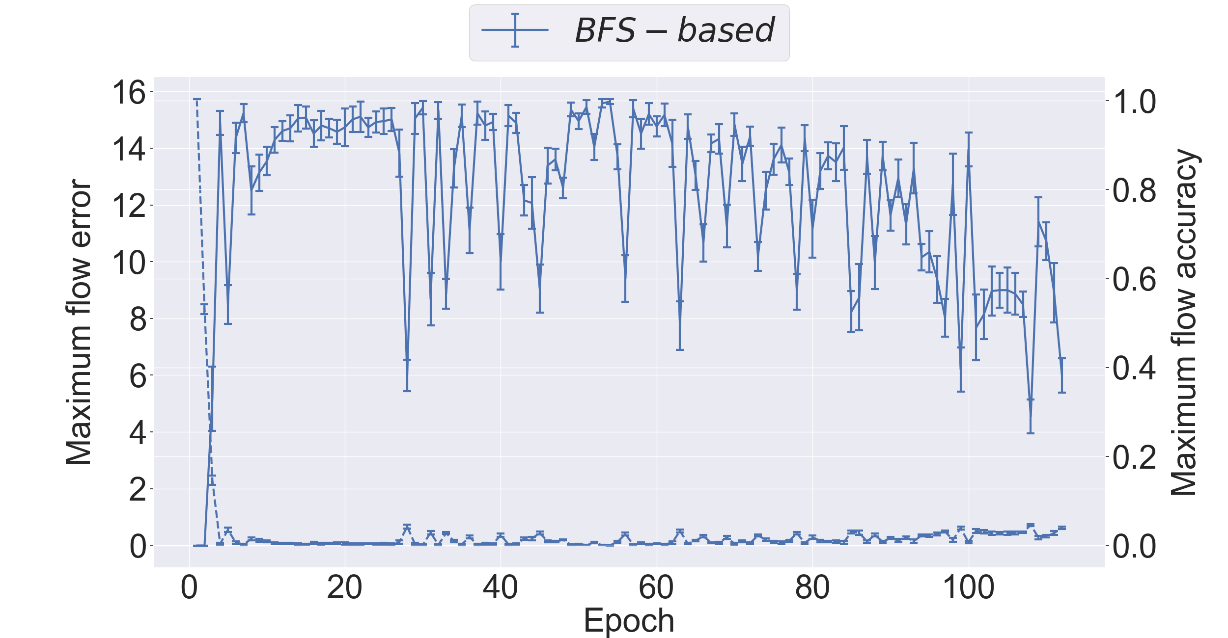
Our initial experiments with the PNA architecture (Table 2) did not align with our expectations – PNA model performs significantly worse than MPNN on the scale. Plotting the accuracy per epoch for that scale reveals that the learner initially starts to converge towards a good solution but it overfits after epoch 25. Our first hypothesis was that since the task of finding maximum flow is deterministic and contains no noise, the std aggregator leads to overfitting. Although removing it did increase the accuracy on the scale, it did not help for strong generalisation, leading to 0% accuracy on larger scales.
We already knew that PNA architecture works when BFS is not used. Hence, our next hypothesis was that since PNA has more parameters and more aggregators (which do not align to the task) than MPNN, extra training data is needed for the BFS task. We provided 200 more bipartite graphs drawn from the same distribution, but had some pairs (up to 40%) of nodes matched greedily. Although BFS still exhibited some instability, as per Figure 2, it stabilised in the last 10-15 epochs, and produced a model which strongly generalised.
Appendix C Varying edge probability
Table 3 shows the accuracy for two best models on data generated with different edge probability . Higher produces cases easily solved by both models. The accuracy is less than 100% mainly for lower edge probability at scale. Both processor architectures perform equivalently data generated with higher edge probability.