How to Project onto an Arbitrary Single-Photon Wavepacket

Abstract

The time-frequency degree of freedom of the electromagnetic field is the final frontier for single-photon measurements. The temporal and spectral distribution a measurement retrodicts (that is, the state it projects onto) is determined by the detector’s intrinsic resonance structure. In this paper, we construct ideal and more realistic positive operator-valued measures (POVMs) that project onto arbitrary single-photon wavepackets with high efficiency and low noise. We discuss applications to super-resolved measurements and quantum communication. In doing so we will give a fully quantum description of the entire photo detection process, give prescriptions for (in principle) performing single-shot Heisenberg-limited time-frequency measurements of single photons, and discuss fundamental limits and trade-offs inherent to single-photon detection.

I POVMs for Photo Detection

Photo detection is at its core an information theoretic process; a measurement outcome—a click—reveals information about the outside world quantifiable in bits Shannon (1948). In the case of a single-photon detector (SPD), a click is correlated (imperfectly) with the presence of a particular type of photon, thus revealing information about the presence of photons of that type along with whatever else in the world such a photon is correlated with. The most general quantum description of this process is in terms of a positive operator-valued measure (POVM), a set of positive operators $\hat{\Pi}_{k}$ that sum to the identity, where each $k$ corresponds to a different measurement outcome. Given an arbitrary input state $\hat{\rho}$ the probability to obtain outcome $k$ is given by the Born Rule

$$Pr(k)={\rm Tr}(\hat{\rho}\hat{\Pi}_{k}).$$ (1)

Generically, each POVM element $\hat{\Pi_{k}}$ can be writen as a weighted sum over orthonormal quantum states

$$\hat{\Pi}_{k}=\sum_{i}w_{i}^{(k)}\left|\phi_{i}^{(k)}\right\rangle\left\langle\phi_{i}^{(k)}\right|$$ (2)

reducing to an ideal Von Neumann measurement only when the sum contains a single term with its weight $w^{(k)}$ equal to $1$ von Neumann (1932). The weight $w_{i}^{(k)}$ equals the conditional probability to obtain measurement outcome $k$ given input $i$. The posterior conditional probability that, given an outcome $k$, we project onto input $i$ is given by Bayes’ theorem Bayes (1763)

$$Pr(i|k)=\frac{w_{i}^{(k)}Pr(i)}{Pr(k)}$$ (3)

with $Pr(k)=\sum_{i}w_{i}^{(k)}Pr(i)$ and $Pr(i)$ the a priori probabilities to get outcome $k$ and for input $i$ to be present, respectively Kraus et al. (1983). Through Bayes’ theorem, an experimentalist is able to retrodict—that is, update their probability distribution over possible inputs—but only if they know what measurement their detector actually performs.

Knowledge of the POVM is essential for both gaining information from a measurement device and characterizing detector performance, hence the experimental need for detector tomography Luis and Sánchez-Soto (1999); Goltsman et al. (2005); Coldenstrodt-Ronge et al. (2009); Lundeen et al. (2009); d’Auria et al. (2011); Brida et al. (2012). Commercial photo detectors are characterized by industry-standard figures of merit Hadfield (2009), which can be calculated from a POVM (for an in-depth review, see Ref. van Enk (2017a)). Here we will concern ourselves mostly with two figures of merit, detection efficiency and time-frequency uncertainty:

Efficiency.—The maximum efficiency with which an SPD outcome $k$ (for instance, a single click) can be triggered by input single photon states is the maximum relative weight in (2) $\eta_{\max}={\rm Max}_{i}[w_{i}^{(k)}]$. The maximum efficiency is achieved only when the input quantum state is one the measurement projects onto. This follows directly from the Born rule; $Pr(k|i)={\rm Tr}[\hat{\Pi}_{k}\hat{\rho}]\rightarrow w_{i}^{(k)}$ if and only if $\hat{\rho}=\left|\phi_{i}^{(k)}\right\rangle\left\langle\phi_{i}^{(k)}\right|$.

Time-Frequency Uncertainty.—The spectral uncertainty and (input-independent) timing jitter are determined entirely by the spectral and temporal widths of the states projected onto by the measurement outcome $k$ Helstrom (1974), which form a retrodictive probability distribution. For any continuous variable $X$ (here either time $t$ or frequency $\omega$), we find it less convenient to use the variance as measure of uncertainty and instead define the uncertainty entropically Helstrom (1974); Bialynicki-Birula and Mycielski (1975); Oppenheim and Wehner (2010); van Enk (2017a); Coles et al. (2019)

$$\Delta X^{(k)}=2^{H^{(k)}_{X}}\delta X.$$ (4)

Here $H^{(k)}_{X}$ is the Shannon entropy defined as

$$H_{X}^{(k)}=-\sum_{j}p(j|k){\rm log}_{2}p(j|k)$$ (5)

with the sum over discretized $X$-bins of size $\delta X$. $p(j|k)$ is the a posteriori probability for the detected photon to be in bin $j$ given outcome $k$, and is calculated

$$p(j|k)=\int_{(j-1)\delta X}^{j\delta X}dX\sum_{i}Pr(i|k)|\phi_{i}(X)|^{2}$$ (6)

where we have defined a normalized distribution over $X$ given by the norm squared of the quantum state $|\phi_{i}(X)|^{2}$ (where $\phi_{i}(X)\equiv\left\langle X|\phi_{i}\right\rangle$). The conditional probability $Pr(i|k)$ is precisely the one from Bayes theorem (3); $Pr(i|k)$ reduces to $w_{i}^{(k)}/\Omega^{(k)}$ in the case of a uniform prior , where $\Omega^{(k)}=\sum_{i}w_{i}^{(k)}$ is the bandwidth van Enk (2017a). Critically, $\Delta X^{(k)}$ is independent of the bin size $\delta X$ in the small-bin limit, even though the entropy $H_{X}^{(k)}$ is strongly dependent on the bin size. One can verify that this definition of uncertainty yields a Fourier time-frequency uncertainty relation Bialynicki-Birula and Mycielski (1975)

$$\Delta\omega\Delta t\geq e\pi.$$ (7)

In this paper, we construct POVMs capable of projecting onto arbitrary quantum states (including minimum-uncertainty Gaussian wavepackets) with high efficiency. The construction of measurements projecting onto arbitrary single-photon states is critical in quantum optical and quantum communication experiments. Mismatch between the single-photon state generated and the state projected onto by the measurement induces an irreversible degradation in detection efficiency. As we show in section II, arbitrary quantum state measurements can be accomplished using a simple time-dependent two-level system. In section III, we show that realistic implementations of minimum-uncertainty POVMs projecting onto arbitrary quantum states are possible, even after including the effects of the initial coupling of the photo detecting system to the external world (transmission), the conversion of a single excitation into a macroscopic signal (amplification), and a noisy classical measurement of that final signal. The capacity to efficiently project onto (a small set of) orthogonal single-photon states enables a wide range of quantum information and quantum optical applications, as we discuss in section IV. In section V, we will discuss the fundamental limits and tradeoffs to photo detector performance that manifest in our work, as well as experimental implementation of the derived POVM (for instance, using a lens to focus light onto a molecule whose state is monitored with electron shelving Dehmelt (1981)) in detail. From a foundational perspective, a procedure to build measurements efficiently projecting onto minimum-uncertainty Gaussian single-photon wavepackets paves the way for future tests of fundamental quantum theory.

II Simplified Measurements Projecting Onto Arbitrary Single-Photon States

We will now discuss how to construct a simple POVM that efficiently projects onto an arbitrary single-photon wavepacket. To aid us, we will now make four simplifying assumptions. First, we will consider only the time-frequency degree of freedom of the electromagnetic field, as the other degrees of freedom (e.g. polarization) can be efficiently sorted prior to detection in a pre-filtering process O’Sullivan et al. (2012); Bouchard et al. (2018); Fontaine et al. (2019). Second, we consider only a single excitation incident to the photo detector. Multiple photons can always be efficiently multiplexed to achieve a photon number resolution using SPD pixels Nehra et al. (2020). Third, we will not model a continuous measurement (as briefly discussed in the appendix of Propp and van Enk (2019a)), but instead a discretized measurement where at a particular time $T$ we ascertain whether or not a photon has interacted with the SPD, ending the measurement. Lastly, we will consider only a binary-outcome photo detector, “click” or “no click.” This simplifies the POVM so that it only contains the two elements $\hat{\Pi}_{T}$ and $\hat{\Pi}_{0}$, both projecting onto the Hilbert space of single photon states and the vacuum state. Generalizations to non-binary-outcome SPDs are straightforward: one can concatenate binary-outcome POVMs to generate non-binary-outcome experiments.

We now begin construction of the POVM $\{\hat{\Pi}_{T},\,\hat{\Pi}_{0}\}$ in earnest. Consider a two-level system with time-dependent transition frequency $\Delta(t)$, with time-dependent coupling to a Markovian external electromagnetic continua of states . Experimentally, a time-dependent decay rate $\kappa(t)$ is induced by a rapid variation of density of states Martínez and Moya-Cessa (2004); Thyrrestrup et al. (2013 ,) and a time-dependent resonance $\Delta(t)$ can be varied with a time-dependent external electric field (Stark effect, Stark (1914)) or through a two-channel Raman transition Law and Eberly (1996).

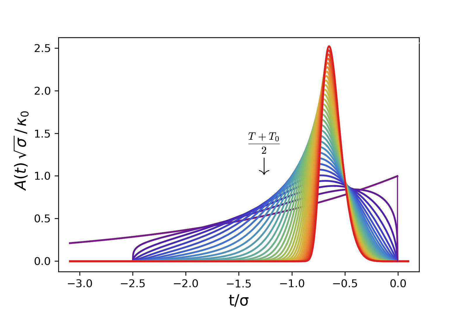
(a)

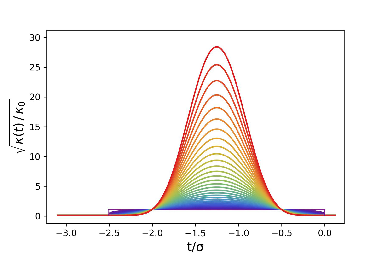
(b)

Figure 1: (a) Retrodictive probability amplitudes $A(t)=|\Psi(t)|$ defined in (12) are plotted for polynomial decays of the form $\kappa(t)=\kappa_{0}\left(\frac{t-T_{0}}{\sigma}\right)^{n}\left(\frac{T-t}{\sigma}\right)^{n}$ for $T_{0}\leq t\leq T$, with the polynomial order $n$ varying from $0$ (violet, lowest peak) to $15$ (red, highest peak) denoted by the color and time measured w.r.t. detection time $T$. (b) The square root of the corresponding decay rates $\sqrt{\kappa(t)}$ are plotted themselves, with polynomial order varying from $0$ (violet, bottom within the central region) to $15$ (red, top within the central region). Except for $n=0$ (also in Fig. 2 and included here for reference), these decays continuously become non-zero at $T_{0}=-2.5\sigma$ (when the photo detector is turned on) so that ${\cal W}$ from (13) is strictly less than unity. In (a), we observe that the time of maximum coupling strength $t=\frac{T+T_{0}}{2}$ precedes the time of maximum retrodictive probability amplitude. For no order $n$ are the retrodictive probability distributions continuously differentiable; measurements with polynomial couplings do not project onto onto smooth wavepackets unlike the couplings plotted in Fig. 3 and Fig. 6.

In the quantum trajectory picture we can assume the state of the two-level system is pure and there are two types of evolution of $\left|\psi(t)\right\rangle$: Schrödinger-like smooth evolution with a non-Hermitian effective Hamiltonian and quantum jumps (at random times) Gardiner et al. (1992); Carmichael (1993). Then the time-dependent (unnormalized) state of the two-level system is written $\left|\psi(t)\right\rangle=C_{0}(t)\left|0\right\rangle+C_{1}(t)\left|1\right\rangle$. A quantum jump will always correspond to the excitation leaking out of the system and so, in the absence of a dark counts, we only need consider the Schrödinger-like evolution in order to determine $\hat{\Pi}_{T}$. In this picture, the quantum state of the two-level system remains pure with the time-dependent excited state amplitude $C_{1}(t)$ obeying a Langevin equation of the form

$$\dot{C}_{1}(t)=-\frac{\kappa(t)}{2}C_{1}(t)-i\Delta(t)C_{1}(t)+\sqrt{\kappa(t)}f(t)$$ (8)

where $f(t)$ is a normalized input photon wavepacket Gardiner and Collett (1985); Gheri et al. (1998). We can solve this equation with the result

$$C_{1}(t)=\int_{T_{0}}^{t}dt^{\prime\prime}f(t^{\prime\prime})\sqrt{\kappa(t^{\prime\prime})}\exp\left[-\int_{t^{\prime\prime}}^{t}dt^{\prime}D(t^{\prime})\right],$$ (9)

where

$$D(t)=i\Delta(t)+\frac{\kappa(t)}{2},$$ (10)

and where $T_{0}$ is a time in the distant past where our photodetector was still off, so that $\kappa(T_{0})=0$ and $C_{1}(T_{0})=0$. Our measurement consists in checking if the system is in the excited state at time $t=T$. The probability to obtain a positive result (corresponding to detecting the incident photon wavepacket) is $|C_{1}(T)|^{2}$. We can write

$$C_{1}(T)=\int_{T_{0}}^{T}dt\Psi^{*}(t)f(t)$$ (11)

with

$$\Psi^{*}(t)=\sqrt{\kappa(t)}\exp\left[-\int_{t}^{T}dt^{\prime}D(t^{\prime})\right].$$ (12)

Whereas $f(t)$ is a normalized wave function, $\Psi(t)$ is subnormalized for finite $T_{0}$, since

$${\cal W}=\int_{T_{0}}^{T}dt|\Psi(t)|^{2}=1-\exp\left[-\int_{T_{0}}^{T}\!dt\,\kappa(t)\right].$$ (13)

$\Psi(t)$ is a complex function with real amplitude $A(t)$ and phase $\phi(t)$ such that $\Psi(t)=A(t)e^{-i\phi(t)}$. We can interpret $|\Psi(t)|^{2}$ as a retrodictive probability distribution over times $t$; indeed, the conditional probability that a photon entered the system between time $t$ and $t+dt$ given a detector “click” at a (later) time $T$ is $Pr(t|T)=|\Psi(t)|^{2}dt$.

We plot in Fig. 1(a) the retrodictive probability distribution amplitudes $A(t)=|\Psi(t)|$ corresponding to simple polynomial decay rates $\kappa(t)=\kappa_{0}\left(\frac{t-T_{0}}{\sigma}\right)^{n}\left(\frac{T-t}{\sigma}\right)^{n}$ for $T_{0}\leq t\leq T$, which are themselves plotted in Fig. 1(b). For $n>0$, these polynomial decay rates incorporate finite response to detector on-time and off-time. We observe that the time of maximum likelihood is determined by competition between two effects, the probability of photo absorption and the rate at which the excited state amplitude decays, both of which are directly determined by $\kappa(t)$. This latter effect drives down the probability amplitude for the distant past. As a result, the peaks of the retrodictive distributions in Fig. 1(a) do not match the peaks of the decay rates in Fig. 1(b) at time $\frac{T_{0}+T}{2}$ (when absorption is highest), but are instead located at a somewhat later time when the two effects balance out. Only a constant $\kappa(t)=\kappa_{0}$ ($n=0$) yields a non-zero probability amplitude at $t=T$ (where it is maximum). For a constant decay rate, the most likely time that a photon entered the system is now whereas for a time-dependent decay rate with $\kappa(T)=0$, there is some time of maximum likelihood determined by competition between the two effects.

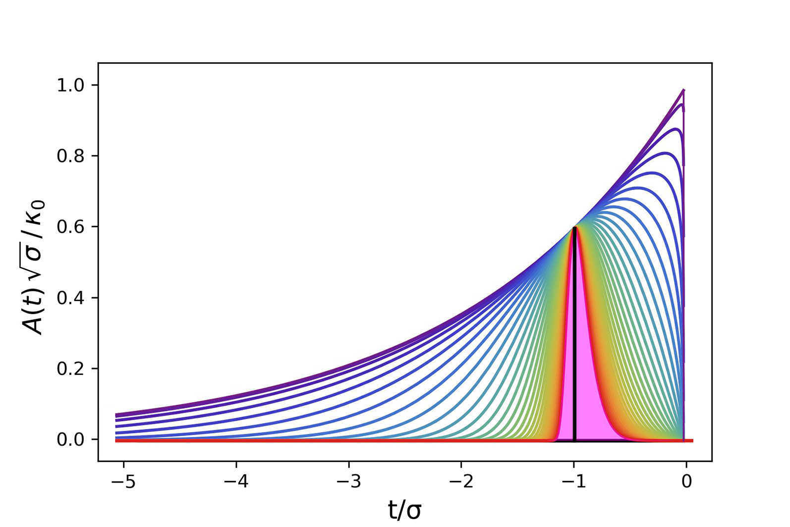
(a)

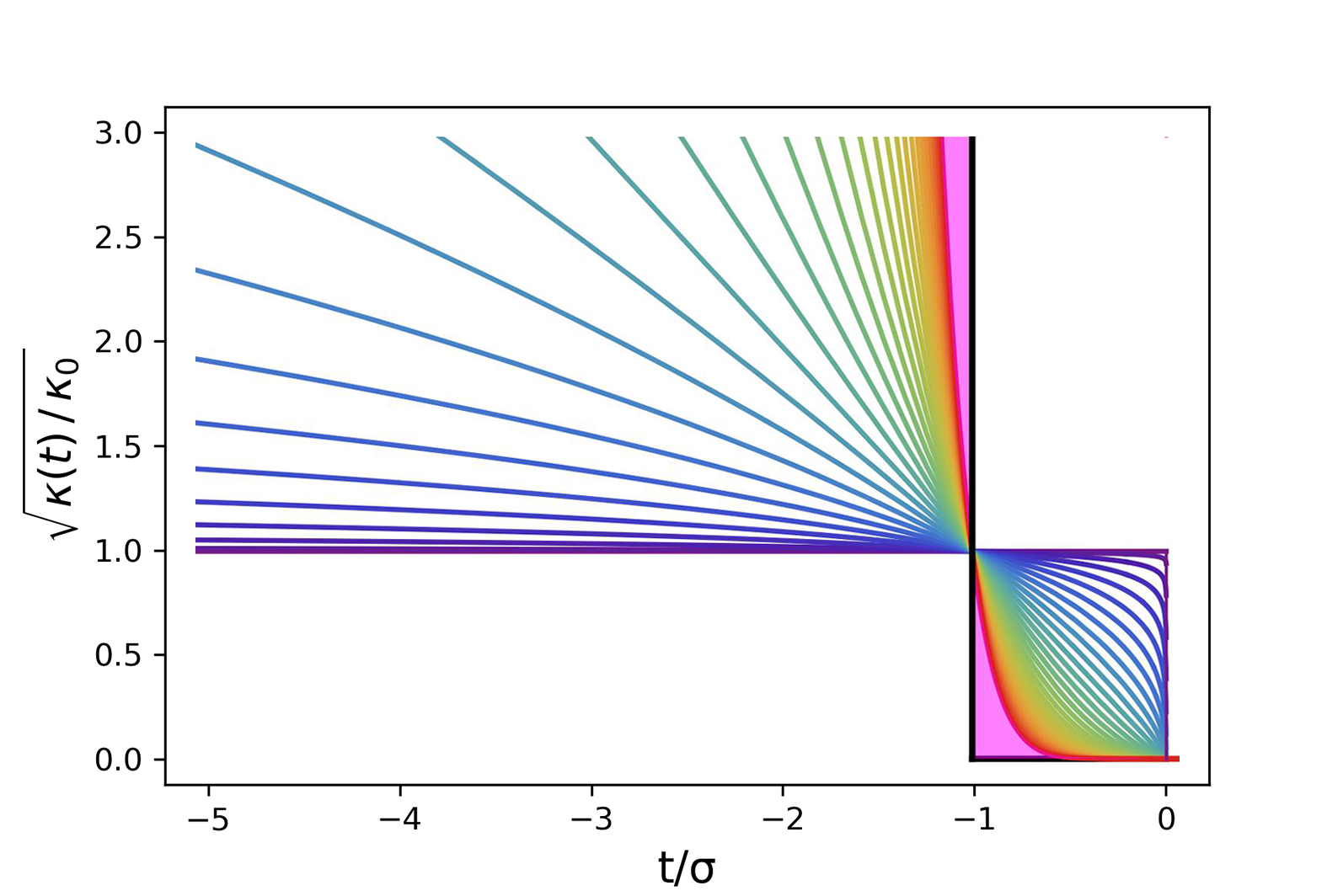
(b)

Figure 2: (a) The retrodictive probability amplitudes $A(t)=|\Psi(t)|$ defined in (12) are plotted for polynomial decays of the form $\kappa(t)=\kappa_{0}\left(\frac{T-t}{\sigma}\right)^{n}$ with polynomial order $n$ varying from $0$ (violet, top) to $15$ (red, bottom) denoted by color. (b) The square root of the corresponding decay rates $\sqrt{\kappa(t)}$ are plotted themselves, with polynomial order varying from $0$ (violet, top for $t/\sigma>-1$) to $15$ (red, bottom for $t/\sigma>-1$). Couplings and retrodictive probability amplitudes for higher polynomial order $n>15$ completely fill in the magenta shaded regions, approaching their asymptotic limits as $n\rightarrow\infty$ (black). In these plots, time is measured w.r.t. time of detection $T$ and we set $T_{0}=-\infty$ so that ${\cal W}=1$ (13). As in Fig. 1, for no order $n>0$ are the retrodictive probability distributions continuously differentiable, and the implemented measurements will not project onto smooth wavepackets unlike those described in Fig. 3 and Fig. 6.

In Fig. 2(a), retrodictive probability distribution amplitudes are plotted for similar polynomial decays of the form $\kappa(t)=\kappa_{0}\left(\frac{T-t}{\sigma}\right)^{n}$ taking into account finite off-time only, plotted in Fig. 2(b). Although for $n>0$ the decay rate $\kappa(t)$ is not normalized and diverges as $t\rightarrow-\infty$, the retrodictive probability amplitudes $A(t)$ generated are still well-behaved. This is because $\kappa(t)$ directly corresponds to the decay rate of the excited state amplitude, so that a large $\kappa(t)$ drives down the probability amplitude for the distant past. As $n$ increases, this divergence in $\kappa(t)$ occurs faster so that for $t-T<\sigma$ the decay rate $\kappa(t)$ is very large, going suddenly to near-zero for $t-T>-\sigma$, completely filling in the shaded region and tending towards the black line for $n\rightarrow\infty$ in Fig. 2(b). These correspond to increasingly narrow retrodictive temporal distributions , filling in the shaded region in Fig. 2(a). Since the decay rate $\kappa(t)$ is very large for $t-T<-\sigma$ an excitation absorbed before $t=-\sigma$ will leak back out, and since the coupling to the continuum $\sqrt{\frac{\kappa(t)}{2\pi}}$ is very small for $t-T>-\sigma$ excitations incident after $t=-\sigma$ will not be absorbed. In the limit $n\rightarrow\infty$ (depicted in Fig. 2 in black), the retrodictive probability distribution is zero everywhere except at $t=-\sigma$—the only time at which an excitation can enter the system and not immediately leak back out.

Having defined a retrodictive probability distribution in (12), we can define a normalized single-photon state

$$\left|\Psi_{T}\right\rangle={\cal W}^{-1/2}\int_{T_{0}}^{T}\!dt\,\Psi(t)\hat{a}^{\dagger}_{\rm in}(t)|{\rm vac}\rangle$$

with the creation operator $\hat{a}^{\dagger}_{\rm in}(t)$ acting on the input continuum of states. The arbitrary input single-photon state (which may have been created long before our detector was turned on at $T_{0}$ or long after the measurement ended at time $T$) is

$$\left|f\right\rangle =\int_{-\infty}^{\infty}dtf(t)\hat{a}^{\dagger}_{\rm in}(t)|{\rm vac}\rangle.$$ (15)

The commutator relation for the input field operator is $[\hat{a}_{\rm in}(t),\hat{a}^{\dagger}_{\rm in}(t^{\prime})]=\delta(t-t^{\prime})$.

The probability for an arbitrary input photon wavepacket $f(t)$ to result in the system being found in the excited state at a time $T$ is $|C_{1}(T)|^{2}={\cal W}\left\langle f|\Psi_{T}\right\rangle\left\langle\Psi_{T}|f\right\rangle$. We rewrite this probability in terms of a POVM element containing a single element

$$\hat{\Pi}_{T}={\cal W}\left|\Psi_{T}\right\rangle\left\langle\Psi_{T}\right|$$ (16)

The positive measurement outcome does not project onto times after we have checked if the system is in the excited state, nor onto times before the detector was turned on. (The other POVM element, describing the no-click outcome, does project onto all times.)

To the extent our detector has been open long enough, such that ${\cal W}\rightarrow 1$, our detector could act as a perfectly efficient detector for a specific single-photon wavepacket with temporal mode function $\Psi(t)$ . This wavepacket is the time reverse of the wavepacket that would be emitted by our two-level system if it started in the upper state $\left|1\right\rangle$ .

For this simple system, the POVM element is both pure (containing just one term ) and (almost) maximally efficient (the weight ${\cal W}$ may approach unity as close as we wish).

Here we observe an obvious trade-off between efficiency and photon counting rate: one cannot project onto a long single-photon wavepacket in a short time interval without cutting off the tails, lowering the overall detection efficiency .

The two-level system described in Eq. (8) is a special case but an important one; the two-level system is often a very good approximation of more complicated systems near-resonance . In this paper, we will focus on the simple time-dependent system (8) as it is sufficiently general to perform a measurement described by any time-independent system, and more . Indeed, (8) is general enough to project onto a completely arbitrary single-photon wavepacket, a result we will now prove.

Proof.— Consider a photon with complex wavepacket $\Psi^{*}(t)=A(t)e^{i\phi(t)}$, positive amplitude $A(t)$, and phase $\phi(t)$. Inserting this into (12), we arrive at two separate expressions

$$A(t) = \sqrt{\kappa(t)}e^{-\int_{t}^{T}dt^{\prime}\frac{\kappa(t^{\prime})}{2}}$$

$$\phi(t) = -\int_{t}^{T}dt^{\prime}\Delta(t^{\prime}).$$ (19)

The second line is always solvable by $\Delta(t)=\dot{\phi}(t)$ up to a constant global phase shift provided $\phi(t)$ is everywhere differentiable (smooth). We now focus on the first line. Taking the natural logarithm we arrive at an expression

$$2{\rm Log}[A(t)]-{\rm Log}[\kappa(t)]=-\int_{t}^{T}dt^{\prime}\kappa(t^{\prime}).$$ (20)

Taking the time derivative of both sides, we arrive at a Bernoulli differential equation Zwillinger (1998)

$$\kappa^{-2}(t)\frac{d\kappa(t)}{dt}-\frac{2}{A(t)\kappa(t)}\frac{dA(t)}{dt}=-1.$$ (21)

Provided $\frac{1}{A(t)}\frac{dA(t)}{dt}$ is continuous, this is solved by

$$\kappa(t)=\frac{A^{2}(t)}{1-\int_{t}^{T}A^{2}(t^{\prime})dt^{\prime}}$$ (22)

Here, $\kappa(t)$ is given by the square of the electromagnetic field, divided by a correction factor accounting for the finite response time imposed by $\kappa(t)$ itself . From (22), we observe that the only condition imposed on $A(t)$ is that $A^{2}(t)$ have an antiderivative. We simply require $A^{2}(t)$ be continuous, which in turn requires $A(t)$ to be continuous. Thus, any wavepacket with smooth phase profile $\phi(t)$ and smooth amplitude $A(t)$ is projected onto by some physically realizable single photon detection scheme. ∎

Special Case: Minimum-Uncertainty Measurement

A minimum-uncertainty simultaneous measurement of time and frequency is achieved with a Gaussian time-frequency distribution. We want a temporal wavepacket $\Psi^{*}(t)$ that is the complex square root a Gaussian distribution

$$\Psi^{*}(t)=\frac{1}{(2\pi\sigma^{2})^{\frac{1}{4}}}e^{\frac{-(t-t_{0})^{2}}{4\sigma^{2}}}e^{i\frac{\omega_{0}}{2}t}$$ (23)

where $\sigma$ is the temporal half-width, and $t_{0}$ and $\omega_{0}$ are the central time frequency of the Gaussian distribution. We find that this wavepacket is projected onto by a time-dependent system with constant resonance $\Delta(t)=\omega_{0}$ and a time-dependent coupling

$$\kappa(t)=\frac{e^{-\frac{(t-t_{0})^{2}}{2\sigma^{2}}}}{\sqrt{2\pi\sigma^{2}}(1+\frac{1}{2}{\rm Erf}[\frac{t_{0}-T}{\sqrt{2}\sigma}]-\frac{1}{2}{\rm Erf}[\frac{t_{0}-t}{\sqrt{2}\sigma}])}$$ (24)

as in Fig. 3. Note that the coupling $\kappa(t)$ is dependent on the time of detection $T$ even though the projected state (23) is $T$-independent, in agreement with the general case (22).

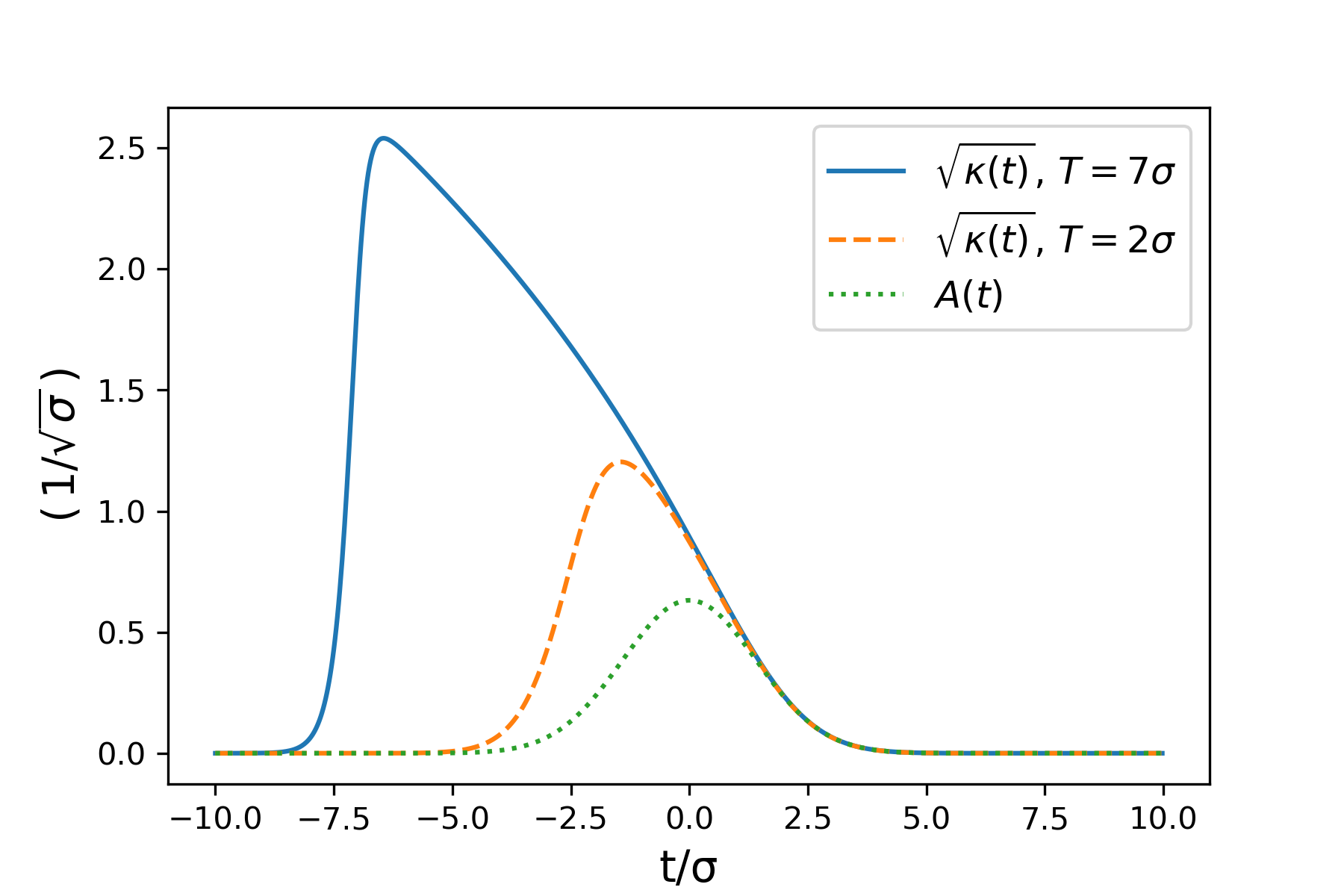
Figure 3: The square root of the time-dependent couplings $\kappa(t)$ defined in (24) generating the minimum uncertainty (Gaussian) wavepacket are plotted for times of detection $T=7\sigma$ (blue solid line, ${\cal W}=1-10^{-10}$) and $T=2\sigma$ (orange dashed line, ${\cal W}=0.98$) in units of $1/\sqrt{\sigma}$ with detector on-time $T_{0}=-\infty$. The retrodictive probability amplitude is now a well-defined wavepacket, with amplitude $A(t)$ (green dotted line) plotted in the rotating frame (without the fast oscillations at the central frequency $\omega_{0}$), also in units of $1/\sqrt{\sigma}$. Time is measured w.r.t. the wavepacket’s central time $t_{0}$. For times near $t\approx T$ the coupling $\sqrt{\kappa(t)}$ is approximately Gaussian as an excitation absorbed at this time will not have sufficient time to decay back out. For earlier times, $\sqrt{\kappa(t)}$ is strictly larger than $A(t)$ and is skewed towards earlier times to incorporate the time it takes the system to respond ($\sim 1/\kappa(t)$); one needs to prepare the two-level system for the photon, accomplished via a “sharkfin” coupling that precedes the single-photon wavepacket Gorshkov et al. (2007). Near $t=-T$, we observe the coupling $\sqrt{\kappa(t)}$ rapidly drops to zero, which is a direct consequence of the temporal wavepacket’s symmetry about $t_{0}$. [From (12) one can quickly verify that, if $A(t)$ is time-symmetric around $t=t_{0}$, the coupling $\kappa(t)$ must satisfy $\kappa(t_{0}-t)=e^{\int_{t_{0}-t}^{t_{0}+t}dt^{\prime}\kappa(t^{\prime})}\kappa(t_{0}+t)$.]

III Realistic Measurements Projecting onto Arbitrary Single-Photon States

The model of a SPD as an isolated two-level system is highly idealized. In a more realistic system, photo detection is an extended process wherein a photon is transmitted into the detector, interacting with the system and triggering a macroscopic change of the photo detector state (amplification) which can then be measured classically. Many theories of single photon detection have been developed over the past century, Glauber (1963); Kelley and Kleiner (1964); Scully and Lamb (1969); Yurke and Denker (1984); Mandel and Wolf (1995); Ueda (1999); Schuster et al. (2005); Helmer et al. (2009); Clerk et al. (2010); Young et al. (2018); Matekole et al. (2018); Léonard et al. (2019) and indeed there are numerous implementations of SPD technology Allen (1939); Lightstone et al. (1981); Marsili et al. (2013); Phan et al. (2014); Wollman et al. (2017). Across all systems, we identify these three stages of transmission, amplification, and measurement as universal. In this section, we derive a POVM that incorporates all three stages quantum mechanically, at the end of the section extending the model to include fluctuations of system parameters. The time-dependent two-level system from the previous section enabling arbitrary wavepacket projection is incorporated into the three-stage model as the trigger for the amplification mechanism. We will assume in this analysis that the system is left on for a sufficient time such that the subnormalization of $\Psi(t)$ is minimal and ${\cal W}\approx 1$ (13).

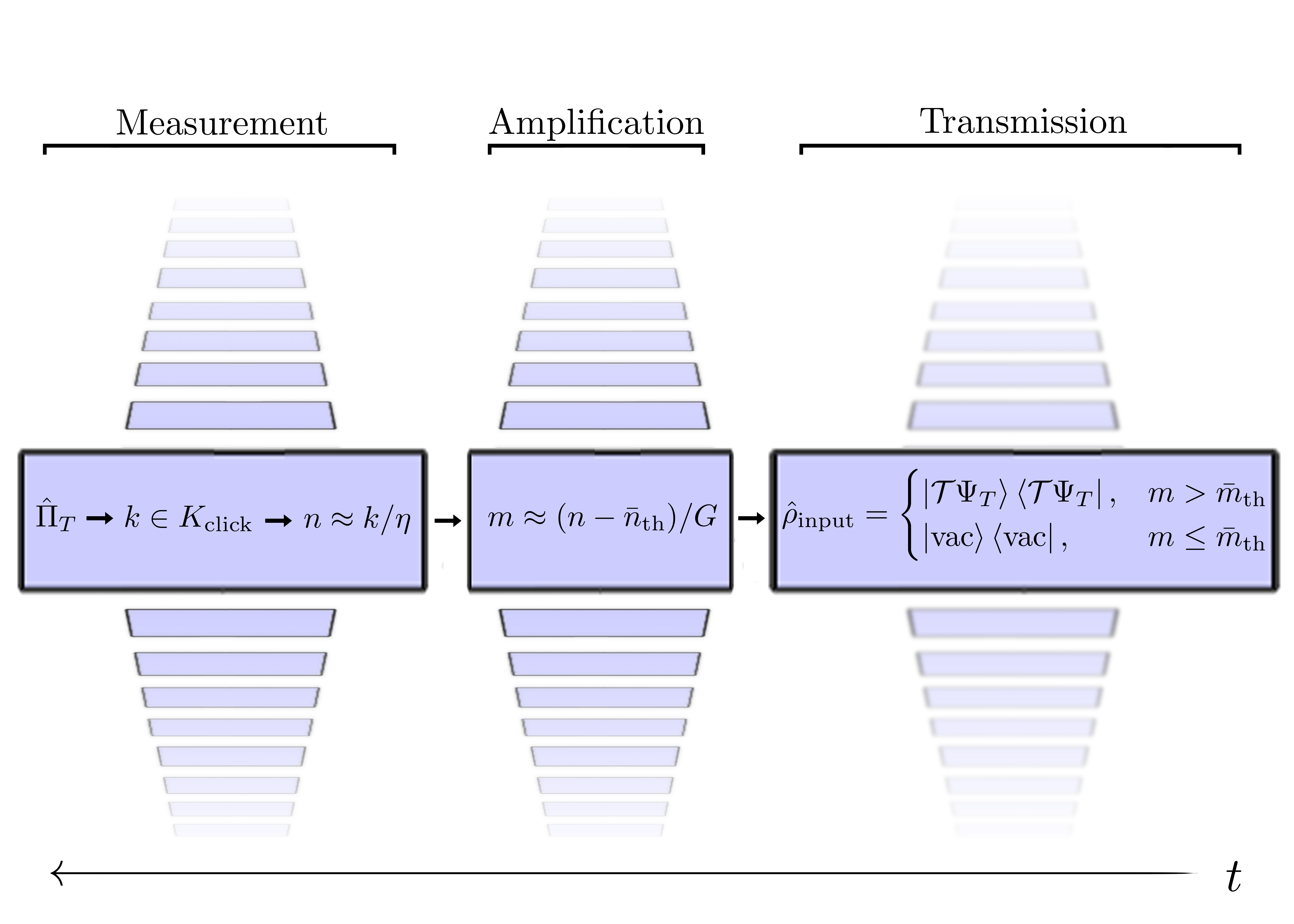
Figure 4: A POVM description of the three-stage model of photo detection, where the chain of inference (left to right) moves opposite the arrow of time, connecting a macroscopic “click” outcome to the state of the input field. A “click” outcome represented by the POVM element $\hat{\Pi}_{T}$ indicates $k\in K_{\rm click}$ excitations were measured post amplification with detection efficiency $\eta$. (Here, we will consider $K_{\rm click}$ to be bounded below by a threshold $k_{\rm min}$ such that $K_{\rm click}=[k_{\rm min},\infty)$.) This suggests $n\approx k/\eta$ (and, strictly, $n\geq k$) excitations were present after in the target mode for amplification. In turn, this indicates that $m\approx(n-\bar{n}_{\rm th})/G\leq n$ excitations were likely incident to the amplification process trigger, with $\bar{n}_{\rm th}$ the expected number of thermal excitations already in the amplification target mode. If $m$ is larger than the expected number of thermal excitations in the amplification trigger mode $\bar{m}_{\rm th}$, we conclude that one (or more) input photon of the form $\left|\mathcal{T}\Psi_{T}\right\rangle\left\langle\mathcal{T}\Psi_{T}\right|$ was likely present. In addition to the states written explicitly, there are other possible states where $k$, $n$, and $m$ deviate from their most likely values. These states (denoted by parallelograms) contribute to the POVM element, as the internal state of the photo detector is in general highly mixed. Nonetheless, in the end a SPD POVM element $\hat{\Pi}_{T}$ only projects onto the two input states $\left|\mathcal{T}\Psi_{T}\right\rangle\left\langle\mathcal{T}\Psi_{T}\right|$ and $\left|\rm vac\right\rangle\left\langle\rm vac\right|$, remaining relatively pure.

In the spirit of what a POVM does (connect present outcomes to probabilistic statements about quantum states in the past), we will begin our endeavor at the very end of the photo detection process following Fig. 4. Consider a macroscopic measurement performed at time $T$ with a binary response triggered by $k$ excitations measured in the amplified signal . Such a POVM can be written as a projector onto Fock states in the Hilbert space internal to the system Barnett2002

$$\hat{\Pi}_{T}=\sum\limits_{k\in K_{\rm click}}\left|k,\,T\right\rangle\left\langle k,\,T\right|.$$ (25)

Here, we have defined an arbitrary set $K_{\rm click}$ that describes how many amplification excitations must be measured to trigger a macroscopic detection event. We will here assume $K_{\rm click}=[k_{\rm min},\infty)$, describing a lower threshold for a photo detection event. At this stage, we can already see that the internal state the POVM projects onto is highly mixed, but this will not directly translate to an impure measurement on the Hilbert space of input photons. Indeed, this is what we would expect; we do not need to know precisely the internal state of the photo detector in order to use it to efficiently detect the presence of a single photon.

The macroscopic measurement performed on the amplified signal will, in general, be inefficient. We model this in a standard way Barnett and Radmore (2002), using a beamsplitter with frequency independent transmission amplitude $\sqrt{\eta}$. We can then rewrite the POVM element (25) so that it projects onto Fock states in the amplification target mode prior to the measurement

$$\hat{\Pi}_{T}=\sum\limits_{k\in K_{\rm click}}\sum\limits_{n=k}^{\infty}\Pr(n|k)\left|n,\,T\right\rangle\left\langle n,\,T\right|$$ (26)

where we have defined

$$\Pr(k|n)={n\choose k}\eta^{k}(1-\eta)^{n-k}$$ (27)

the probability to detect $k$ excitations given that there were $n$ excitations in the output mode of the amplification process, which is the same as $Pr(n|k)$ (the probability that given $k$ detected excitations $n$ excitations were incident, needed in (26)) in the absence of prior information . An inefficiency $1-\eta$ affects photo detection by changing which post-amplification Fock states are projected onto: for a larger $1-\eta$ the distribution of post-amplification states $\left|n,\,T\right\rangle\left\langle n,\,T\right|$ that contribute to the final outcome $\hat{\Pi}_{T}$ becomes larger. This increases the overlap between $\hat{\Pi}_{T}$ and the null outcome $\hat{\Pi}_{0}$, so that it is harder to distinguish between signal and noise (dark counts).

We now move one step further back in the chain of inference (Fig. 4) so the POVM element $\hat{\Pi}_{T}$ projects onto the number of excitations $m$ input to the amplification trigger. Amplification is a generic feature of photo detection; without a macroscopic change in the internal state of a photo detector, there is no way to correlate detector outcomes with the presence of a single photon Yang and Jacob (2018, 2019, 2020) (that is, without invoking additional single-excitation detectors in an argument circulus in probando). There are many interesting methods for implementing amplification Caves (1982); Imamoḡlu (2002); Gavish et al. (2004); Clerk et al. (2010); Metelmann and Clerk (2014); Yang and Jacob (2018, 2019, 2020), but the fundamental quantum limit to amplification of any bosonic Fock state is achieved by a Schrödinger picture transformation Propp and van Enk (2019b)

$$\left|m\right\rangle_{\rm trig}\left|M\right\rangle_{\rm res}\left|N\right\rangle_{\rm targ}\longmapsto\left|m\right\rangle_{\rm trig}\left|M-Gm\right\rangle_{\rm res}\left|N+Gm\right\rangle_{\rm targ}$$

such that exactly $G$ excitations are transferred from the reservoir mode to the target mode for each excitation in the trigger mode. In using this expression we do impose a restriction that there must be $M>Gn$ excitations in the reservoir mode, but restrictions of this type are to be expected (the energy for amplification must come from somewhere) and we will be most interested in few photons ($n=0,1,2$) in this analysis. In most physical platforms $G$ will fluctuate , as will other (classical) system parameters which we will return to at the end of this section. (Exceptions do exist; for Hamiltonians that implement deterministic amplification schemes [with small integer values for $G$] see Ref. Björk et al. (1998).) However, even with a definite gain factor $G$ and number of input excitations $m$, we will still not end up with exactly $n=N+Gm$ excitations if the target mode is initially in a thermal state with mean occupation number $\bar{N}$ (as opposed to a Fock state with exactly $N$ excitations). We now assume this, writing the state of the target mode in the Fock basis

$$\hat{\rho}_{\rm targ}^{(th)}=\sum\limits_{N=0}^{\infty}P^{\rm th}_{N,\,T}|N,\,T\rangle\!\langle N,\,T|,$$ (29)

with the probability for $N$ thermal excitations given by

$$P^{\rm th}_{N}=\frac{1}{1+\bar{N}}\left(\frac{\bar{N}}{1+\bar{N}}\right)^{N};\,\bar{N}=\frac{1}{e^{\frac{\hbar\omega^{\prime}}{\tau}}-1},$$ (30)

where $\omega^{\prime}$ and $\tau$ are the frequency and the fundamental temperature of the target mode. Assuming the ideal amplification scheme in (III), we now write the POVM element $\hat{\Pi}_{k}$ in terms of the number $m$ excitations that trigger the application mechanism

$$\!\hat{\Pi}_{T}=\sum\limits_{k\in K_{\rm click}}\sum\limits_{n=k}^{\infty}\Pr(n|k)\sum\limits_{m=0}^{{\rm Fl}[\frac{n}{G}]}P^{\rm th}_{n-Gm}\left|\Psi_{T}\right\rangle\left\langle\Psi_{T}\right|^{\otimes m}$$

where we define $\left|\Psi_{T}\right\rangle\left\langle\Psi_{T}\right|^{\otimes 0}=|{\rm vac}\rangle\langle{\rm vac}|$ and $P^{\rm th}_{N}=0$ for $N<0$ and have introduced the floor function ${\rm Fl}[x]={\rm Max}[n\in\mathbb{Z}\,|\,n\leq x]$. We can now see the benefit of having a large gain factor G; it shifts the probability distribution over $n$ that corresponds to non-zero excitations in the trigger mode, minimizing its overlap with the probability distribution for zero excitations. In this way, one can dramatically reduce the background noise (dark counts) without decreasing signal by changing ${\rm Min}[K_{\rm click}]$. In (III) we have reintroduced the state $\left|\Psi_{T}\right\rangle$ defined in (II) as the state described by projected onto by the trigger mechanism. As we did in the previous section, we will assume a time-dependent resonance frequency $\Delta(t)$ and decay rate $\kappa(t)$ so that arbitrary pulse-shaping is possible.

The POVM element in (III) now projects onto quantum states internal to the photo detector. We need to connect the internal continuum of states coupled to the amplification trigger to the external continuum containing the photons we wish to detect (the transmission stage in Fig. 4). This is accomplished by introducing an arbitrary two-sided quantum network Propp and van Enk (2019a). This is completely described by a single complex frequency-dependent transmission coefficient $\mathcal{T}(\omega)$ (related to a reflection coefficient at each frequency via $|\mathcal{T}(\omega)|^{2}+|\mathcal{R}(\omega)|^{2}=1$ and $\mathcal{R}(\omega)\mathcal{T}^{*}(\omega)+\mathcal{R}^{*}\omega)T(\omega)=0$). We now invoke the single-photon assumption so that there is at most a single excitation input to the quantum network. Any other excitations present in the internal continua will be from internally-generated thermal fluctuations reflected by the quantum network back to the trigger mechanism. In this way, we can construct a POVM element that projects onto product-states $\left|\psi_{\rm ex}\right\rangle\left\langle\psi_{\rm ex}\right|\otimes\left|\psi_{\rm in}\right\rangle\left\langle\psi_{\rm in}\right|$ of the external and internal continua

$$\hat{\Pi}_{T} = \sum\limits_{k\in K_{\rm click}}\sum\limits_{n=k}^{\infty}\Pr(n|k)\left(P^{\rm th}_{n}|{\rm vac}\rangle\langle{\rm vac}|\otimes|{\rm vac}\rangle\langle{\rm vac}|+\sum\limits_{m=1}^{{\rm Fl}[\frac{n}{G}]}P^{\rm th}_{n-Gm}\beta^{2m}|{\rm vac}\rangle\langle{\rm vac}|\otimes\left|\mathcal{R}\Psi_{T}\right\rangle\left\langle\mathcal{R}\Psi_{T}\right|^{\otimes m}\phantom{\sum\limits_{m=1}^{{\rm Fl}[\frac{n}{G}]}}\right.$$

$$+ \left.\sum\limits_{m=1}^{{\rm Fl}[\frac{n}{G}]}mP^{\rm th}_{n-Gm}\alpha^{2}\beta^{2(m-1)}\left|\mathcal{T}\Psi_{T}\right\rangle\left\langle\mathcal{T}\Psi_{T}\right|\otimes\left|\mathcal{R}\Psi_{T}\right\rangle\left\langle\mathcal{R}\Psi_{T}\right|^{\otimes m-1}\right).$$

The first term corresponds to dark counts generated from thermal excitations post-amplification and the second term corresponds to dark counts generated by thermal excitations that then trigger the amplification mechanism. Only the third term contains a projection onto a photon to be detected. (The multiplicative factor $m$ in the third term is combinatorial in origin: $m$ total excitations in the trigger mode with $m-1$ generated from thermal fluctuations.) In writing (III) we have defined transmitted and reflected normalized single-photon states and coefficients

$$\left|\mathcal{T}\Psi_{T}\right\rangle = \frac{1}{\alpha}\int_{-\infty}^{\infty}\,d\omega\tilde{\Psi}(\omega)\mathcal{T}^{*}(\omega)e^{i\,\omega\,T}\hat{a}^{\dagger}(\omega)\left|\textnormal{vac}\right\rangle$$

$$\left|\mathcal{R}\Psi_{T}\right\rangle = \frac{1}{\beta}\int_{-\infty}^{\infty}\,d\omega\tilde{\Psi}(\omega)\mathcal{R}^{*}(\omega)e^{i\,\omega\,T}\hat{b}^{\dagger}(\omega)\left|\textnormal{vac}\right\rangle$$

$$\alpha = \sqrt{\int d\omega|\tilde{\Psi}(\omega)|^{2}|\mathcal{T}(\omega)|^{2}}$$

$$\beta = \sqrt{\int d\omega|\tilde{\Psi}(\omega)|^{2}|\mathcal{R}(\omega)|^{2}}$$ (33)

where $\hat{a}^{\dagger}$ and $\hat{b}^{\dagger}$ are the creation operators for the external and internal continua and we have defined a Fourier-transformed wavepacket for the amplification trigger mode $\tilde{\Psi}(\omega)={\rm FT}[\sqrt{\kappa(t)}\Psi(t)]$. We can now see how pre-amplification dark counts (the second line of (III)) can be suppressed: by reducing the overlap of $|\tilde{\Psi}(\omega)|^{2}$ and $|\mathcal{R}(\omega)|^{2}$, that is, by only amplifying the frequencies we wish to detect so that $\beta^{2}\ll 1$. In this case, the POVM element (III) will be dominated by the $m=1$ term of the third line (the signal to be detected with no thermal excitations), as well as potentially the first line. (To reiterate, these are dark counts post-amplification, but these can be reduced by amplifying at a high frequency such that $\hbar\omega^{\prime}\gg\tau$, where $\omega^{\prime}$ and $\tau$ are the frequency and fundamental temperature of the target mode.)

Finally, we trace over the internal continua, which we assume is in a thermal state with fundamental temperature $\tau^{\prime}$ so the POVM projects onto the external continua only

$$\hat{\Pi}_{T} = \sum\limits_{k\in K_{\rm click}}\sum\limits_{n=k}^{\infty}\Pr(n|k)\left(\sum\limits_{m=0}^{{\rm Fl}[\frac{n}{G}]}P^{\rm th}_{n-Gm}P^{{}^{\prime}\rm th}_{m}\beta^{2m}\right.|{\rm vac}\rangle\langle{\rm vac}|$$ (34)

$$+ \left.\sum\limits_{m=1}^{{\rm Fl}[\frac{n}{G}]}mP^{\rm th}_{n-Gm}P^{{}^{\prime}\rm th}_{m-1}\alpha^{2}\beta^{2(m-1)}\left|\mathcal{T}\Psi_{T}\right\rangle\left\langle\mathcal{T}\Psi_{T}\right|\right)$$

$$\equiv w_{0}|{\rm vac}\rangle\langle{\rm vac}|+w_{T}\left|\mathcal{T}\Psi_{T}\right\rangle\left\langle\mathcal{T}\Psi_{T}\right|$$

where in the last line we have absorbed the sums in front of the two projectors into weights so that the POVM element has the form of (2) and with $P^{{}^{\prime}\rm th}_{j}$ the probability to have $j$ thermal excitations (now in the non-monochromatic reflected mode defined in (III)). For a finite detector on-time $T_{0}>-\infty$, the weights $w_{0}$ and $w_{T}$ will be slightly less than in (34) due to wavepacket sub-normalization (13). However, this deviation is negligible provided the detector is left on for a time comparable to the temporal mode’s width.

We now reconsider the question of projecting onto an arbitrary wavepacket, including the full quantum description. We find that this is possible to do in principle, provisio $\mathcal{T}(\omega)$ is nowhere zero (except at infinity), a result we will now prove. That is, we can ensure that the single-photon wavepacket $\left|\mathcal{T}\Psi_{T}\right\rangle$ has any desired (smooth) shape and will be projected onto with a high-efficiency and high-purity measurement.

Proof.—Consider a photon with complex normalized spectral wavepacket $\tilde{f}(\omega)$. If detection is achieved with a time-dependent two-level system preceded by a quantum network with filtering transmission function $\mathcal{T}(\omega)$, the system will project onto a state $\left|\mathcal{T}\Psi_{T}\right\rangle$ as defined in (III). In the low-noise limit this will be the only state projected onto by the (pure) POVM element. From the Born rule, the probability of detection will be

$$P_{T}=w_{T}\frac{1}{\alpha^{2}}\left|\int_{-\infty}^{\infty}d\omega\tilde{f}(\omega)\tilde{\Psi}(\omega)\mathcal{T}^{*}(\omega)\right|^{2}$$ (35)

with $w_{T}$ the overall weight given by (34) and maximum possible detection efficiency, which can be arbitrarily close to unity. It is possible to achieve $P_{T}=w_{T}$ (mode-matched detection) in (35) if and only if

$$\tilde{\Psi}(\omega)=\frac{\tilde{f}^{*}(\omega)}{\mathcal{T}(\omega)}e^{i\omega T}.$$ (36)

From (12), we know that it is possible to generate an arbitrary temporal wavepacket ${\rm FT}^{-1}[\tilde{\Psi}(\omega)]=\sqrt{\kappa(t)}\Psi(t)$ from a time-dependent two-level system. The Fourier transform of a continuous smooth function is itself smooth and continuous. Thus, if the right hand side of (36) is a well-defined spectral wavepacket (smooth and continuous), one can find functions $\kappa(t)$ and $\Delta(t)$ such that $\tilde{\Psi}(\omega)$ has the form of (36). ∎

Remark.— Arbitrary wavepacket detection (and thus Heisenberg-limited simultaneous measurements of time and frequency) is in principle possible only when there are no photonic band gaps induced by the filter; if $\mathcal{T}(\omega^{\prime})=0$ for some frequency $\omega^{\prime}$, there is simply no way to compensate for the lost information about $\omega^{\prime}$. Photonic band gaps are a generic feature of parallel (and hybrid) quantum networks Propp and van Enk (2019a) as well as certain non-Markovian systems Garraway and Dalton (2006). Network/reservoir engineering must be employed to ensure any $\omega^{\prime}$ where $T(\omega^{\prime})=0$ is not a frequency of interest.

The POVM $\{\hat{\Pi}_{T},\,\hat{\Pi}_{0}\}$ with $\hat{\Pi}_{T}$ defined in (34) and $\hat{\Pi}_{0}=\hat{\mathds{1}}-\hat{\Pi}_{T}$ provides a complete description of the single photon detection process that is fully quantum from beginning to end (Fig. 4). However, there is a final element that must be considered to make the description applicable to laboratory systems: classical parameter fluctuations. For continuous parameter fluctuations over any system parameter or set of system parameters $X$, these are naturally incorporated

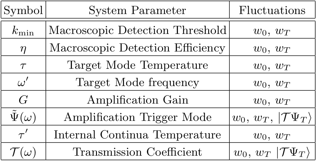
Figure 5: The effects of classical fluctuations in system parameters on the final POVM: either the weights and states are changed, or only the weights are changed. The fluctuations over the functions $\tilde{\Psi}(\omega)$ and $\mathcal{T}(\omega)$ (and thus $\mathcal{R}(\omega)$ by unitarity) could be caused by fluctuations in other system parameters (decay rates, resonances) internal to those functions. A subset of fluctuations in $\tilde{\Psi}(\omega)$ are fluctuations in the time of detection $T$. Importantly, these shift the wavepacket $\Psi(t)$ projected onto, resulting in a mixed measurement with larger temporal uncertainty (jitter) that depends on the ratio of the fluctuations in $T$ to the width of the temporal wavepacket.

$$\!\hat{\Pi}_{T}=\int dX{\rm Pr}(X)\left(w_{0}|{\rm vac}\rangle\langle{\rm vac}|+w_{T}\left|\mathcal{T}\Psi_{T}\right\rangle\left\langle\mathcal{T}\Psi_{T}\right|\right)$$

where we have assumed a (known) probability distribution ${\rm Pr}(X)$. In (III), the system parameter(s) $X$ could be such that only the weights $w_{0}$ and $w_{T}$ depend on $X$, or $X$ could be such that the state $\left|\mathcal{T}\Psi_{T}\right\rangle$ depends on $X$ as well (for a summary, see Fig. 5). In the case of the latter, the POVM will become less pure and will need rediagonalization to determine which states are projected onto . This final POVM not only includes ignorance about the internal state of the photo detector as was depicted in Fig. 4, but also classical ignorance about the state of the photo detector due to system-lab interactions.

For example, let us start with our ideal detector from Section II, which projects onto a Gaussian wave packet (23) with a central time $t_{0}$ a fixed duration before $T$ and a width $\sigma$ determined by the specific form of $\kappa(t)$. Suppose the parameter $T$ fluctuates such that $t_{0}$ fluctuates but $\sigma$ stays fixed. For definiteness, assume a Gaussian distribution for the central time $\tau_{0}$ of the wave packet

$${\rm Pr}(\tau_{0})=\frac{1}{\sqrt{2\pi w^{2}}}\exp(-(\tau_{0}-t_{0})^{2}/2w^{2})$$ (38)

with $w$ the width of that distribution. One effect on the POVM “click” element of this uncertainty about the value of $\tau_{0}$ is that its purity decreases. Since that consequence has been discussed in a slightly different context in Ref. van Enk (2017b), we focus here on a second effect: that the probability of detecting the single-photon wave packet (23) our detector was designed to detect perfectly decreases. The probability to detect our favorite wave packet given a parameter $\tau_{0}$ is

$${\rm Pr}(t_{0}|\tau_{0})=\exp(-(\tau_{0}-t_{0})^{2}/4\sigma^{2}).$$ (39)

Averaging this probability over the Gaussian distribution over $\tau_{0}$ gives

$$\int\!d\tau_{0}\,{\rm Pr}(\tau_{0}){\rm Pr}(t_{0}|\tau_{0})=\frac{1}{\sqrt{1+(w/\sigma)^{2}/2}},$$ (40)

which in the limit of $w\rightarrow 0$ reaches 1, as it should, and which for large $w$ decays to zero as $\sqrt{2}\sigma/w$. If one additionally includes other realistic factors (finite temperature, finite gain, and the threshold value $k_{\rm min}$ of $K_{\rm click}=[k_{\rm min},\infty)$), the conditional probability ${\rm Pr}(t_{0}|\tau_{0})$ remains uniform across the parameter $\tau_{0}$ and thus the overall detection efficiency decreases by the factor $w_{T}$ as defined in (34).

We may take this description one step further and consider $X$ not as a set of classical parameters but as (discrete) outcomes $X_{n}$ of quantum measurements. That is, there is a higher-level POVM $\pi_{n}$ describing measurements on one or more auxiliary system (e.g., a quantum clock for measuring time Maccone and Sacha (2020)), with the possible outcomes labeled by the parameters $X_{n}$. When the probability of the measurement outcome $X_{n}$ is ${\rm Pr}(X_{n})$, then we would get the same type of mixed POVM (III)—but with the integral replaced by a sum over $n$—when different outcomes correspond to orthogonal outcomes of a standard Von Neumann measurement, such that ${\rm Tr}(\pi_{n}\pi_{m})=\delta_{nm}$. In case different outcomes are not orthogonal (as would be the case for quantum measurements of phase and time), the probability distribution ${\rm Pr}(X)$ must be replaced according to

$$\int\!dX\,{\rm Pr}(X)\hat{\Pi(X)}\longmapsto\sum_{n}\sum_{m}\frac{{\rm Tr}(\pi_{n}\pi_{m})}{{\rm Tr}(\pi_{m})}{\rm Pr}(X_{m})\hat{\Pi}(X_{n}),$$ (41)

since an outcome $\pi_{m}\neq\pi_{n}$ may still project onto the single-photon state corresponding to $X_{n}$. Apart from this change the result (III) retains the same form.

IV Applications

Using the time-dependent two-level system, we are able to project onto orthogonal quantum states (Fig. 6). This enables efficient detection of photonic qubits, an essential component of any quantum internet Kimble (2008); Lukens and Lougovski (2017). More generally, temporal modes provide a complete framework for quantum information science Brecht et al. (2015), with efficient detection of orthogonal modes (and their superpositions to create mutually unbiased bases) a key ingredient. Fully manipulable temporal modes also play a key role in error-corrected quantum transduction Enk et al. (1997), where a time-reversed temporal mode can restore an unknown superposition in a qubit. Here, efficient detection of arbitrary temporal modes is essential so that quantum jumps out of the dark state are efficiently heralded.

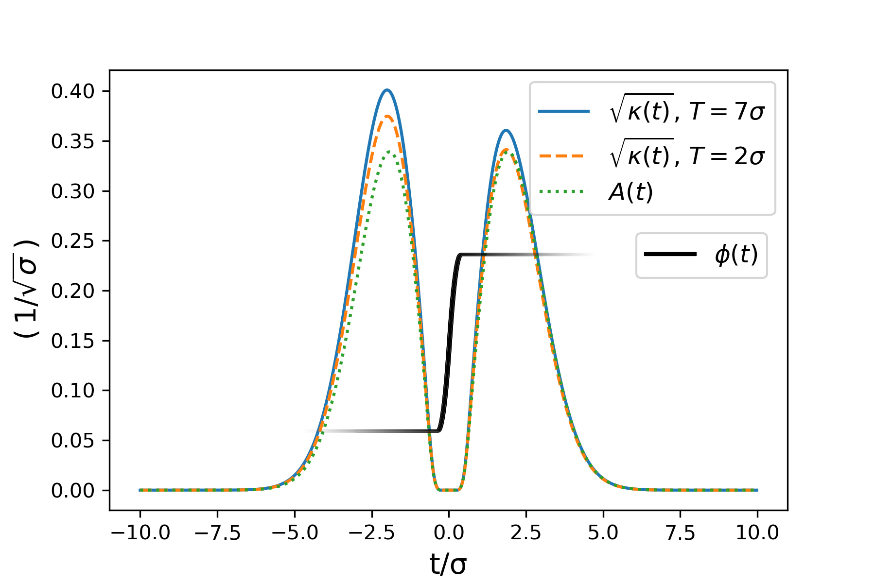
Figure 6: The time-dependent coupling $\kappa(t)$ that generates a wavepacket exactly orthogonal to the minimum uncertainty Gaussian wavepacket in Fig. 3 are plotted in units of $1/\sqrt{\sigma}$ for times of detection $T=7\sigma$ (solid blue line, ${\cal W}=1-10^{-5}$) and $T=2\sigma$ (dashed orange line, ${\cal W}=0.72$) and detector on-time $T_{0}=-\infty$. In the rotating frame, the wavepacket’s time-dependent amplitude $A(t)$ (green dotted line, also in units of $1/\sqrt{\sigma}$) is an approximate first-order Hermite-Gaussian pulse, where the singular region of zero has been expanded with half-width of $z=0.5\sigma$. In this way, the wavepacket’s phase (thick black line, not to scale) can go from $0$ to $\pi$ in a finite time, whereas the Heaviside phase-flip in the exact Hermite-Gaussian pulse requires an unphysical delta-function detuning (second line of (II). Both the phase and amplitude have been convolved with a triangular smoothing function with full-width $s=0.5\sigma$, ensuring $A(t)$ is continuously differentiable to first order Boehme and Bracewell (1966); de Boor (1972), which is pre-requisite for solving the Bernoulli equation (21). For any finite $z\geq s>0$ the phase flip [here implemented with a triangular detuning $\Delta(t)$] occurs while the amplitude is zero. This ensures exact orthogonality of the approximate first-order Hermite-Gaussian to the gaussian pulse. In the limit $s,z\rightarrow 0$, an exact first-order Hermite-Gaussian is recovered. This smoothing procedure generalizes to higher order Hermite-Gaussian pulses, forming a mutually unbiased basis for efficient detection of higher dimensional qudits Brecht et al. (2015).

High-purity measurements that project onto orthogonal single-photon wavepackets also enable super-resolved measurements Chrostowski et al. (2017). Suppose we have two single-photon sources emitting almost identical pure states differing slightly in either emission time or central frequency

$$\left|\tilde{\phi}_{1}\right\rangle =\frac{\left|\phi_{1}\right\rangle+\sqrt{\epsilon}\left|\phi_{2}\right\rangle}{\sqrt{1+\epsilon}}$$

$$\left|\tilde{\phi}_{2}\right\rangle =\frac{\left|\phi_{1}\right\rangle-\sqrt{\epsilon}\left|\phi_{2}\right\rangle}{\sqrt{1+\epsilon}}$$ (42)

with $\left\langle\tilde{\phi}_{1}|\tilde{\phi}_{2}\right\rangle$ real, $\epsilon\ll 1$, and $\left\langle\phi_{1}|\phi_{2}\right\rangle=0$. Alternatively, we may imagine a single source of light but the light we receive may have either been slightly Doppler-shifted or it may have been slightly delayed.

Suppose now that we receive one photon that could equally likely be from either source so that our input state is

$$\hat{\rho}=\frac{1}{2}\left|\tilde{\phi}_{1}\right\rangle\left\langle\tilde{\phi}_{1}\right|+\frac{1}{2}\left|\tilde{\phi}_{2}\right\rangle\left\langle\tilde{\phi}_{2}\right|.$$ (43)

If we can measure both $\hat{\Pi}_{1}=\eta\left|\phi_{1}\right\rangle\left\langle\phi_{1}\right|$ and $\hat{\Pi}_{2}=\eta\left|\phi_{2}\right\rangle\left\langle\phi_{2}\right|$ (that is, if we have separate photodetectors with these (pure) POVM elements, or a single non-binary-outcome photo detector), then we find the probability of clicks

$$P_{1} = {\rm Tr}\left[\hat{\Pi}_{1}\hat{\rho}\right]=\eta\frac{1}{1+\epsilon}$$

$$P_{2} = {\rm Tr}\left[\hat{\Pi}_{2}\hat{\rho}\right]=\eta\frac{\epsilon}{1+\epsilon}$$ (44)

so that the ratio of clicks gives a direct estimate of $\epsilon$, even for low efficiency $\eta$. Here all that is needed for time-frequency domain super-resolved measurement of $\epsilon$ are SPDs with time-dependent couplings and resonance frequencies as opposed to nonlinear optics Donohue et al. (2018).

In traditional quantum key distribution (QKD) schemes (that is, not measurement device independent (MDI)-QKD), specification of the measurement POVM is essential to robust security proofs Tamaki and Lütkenhaus (2004); Qi (2006); Fung et al. (2009). Here, we have verified several assumptions about an eves-dropper’s capabilities common in security proofs: that high-purity measurements are possible, that high efficiency measurements are possible, and (for continuous-variable (CV)-QKD proofs) minimum time-frequency uncertainty measurements are possible. In particular for CV-QKD, an eavesdropper can perform measurements that project onto variable-width spectral modes, disrupting temporal correlations between Alice and Bob (who are assumed to use fixed time-frequency bins) Bourassa and Lo (2019). Here, the capacity to adjust the width of the spectral mode $\tilde{\Psi}(\omega)$ provides Alice and Bob a new strategy to mitigate Eve’s attack and extract a secure key.

More generally, detector tomography is an important tool across implementations of single-photon and number-resolved photo detection D’Ariano et al. (2004); Lundeen et al. (2009); Coldenstrodt-Ronge et al. (2009); Ma et al. (2016). Real-time tomography could be useful in QKD protocols resistant to “trojan-horse attacks” Gisin et al. (2006) or any SPD platform subject to time-dependent environmental parameter fluctuations: for instance, atmospheric turbulence in MDI-QKD Hu et al. (2018) or interplanetary medium in deep space classical communications Banaszek et al. (2019). Recently tomography speed-ups have been achieved using machine learning assisted tomography protocols Melkani et al. (2019). The POVMs derived in this paper provide priors which can further speed up detector tomography Heinosaari et al. (2013). These include approximate effects of environmental fluctuations as outlined in Fig. 5 and a global optimum POVM for single photon detection (34) which can be used to incorporate detector calibration and optimization into in situ tomographic protocols.

V Conclusions

Having gone through applications of our work, we return to the fundamental (as opposed to practial) limits to single photon detection and their implications, as well as possible experimental implementations.

Here we have constructed single-photon measurements that are Heisenberg-limited in two ways: the first is that they can project onto Gaussian time-frequency states as illustrated in Fig. 3, and the second is that the amplification scheme reaches a Heisenberg-limited (linear in the gain $G$) signal-to-noise ratio, surpassing the standard quantum limit (a signal-to-noise ratio going like of $\sqrt{G}$) Propp and van Enk (2019b). Achieving these simultaneously is possible in principle with no drawback. Indeed, the only stringent tradeoff we encounter in this analysis is between efficiency and photon counting rate, which becomes substantial when an SPD is reset at a faster rate than $\sim 1/\Delta t$. (The photon does not have sufficient time to excite the two-level system with high probability before the system is reset.) For other figures of merit, we find that they are either independent, or deteriorate together . While it does appear from (34) that improving efficiency also increases dark counts, these are decoupled by ensuring the coefficient $\beta\ll 1$—that is, by making $\mathcal{T}(\omega)$ broader than $\tilde{\Psi}(\omega)$ as in (III). While it is commonsense that one should only amplify the frequencies they wish to detect, our work clarifies how enormously important this is. The dark counts produced in this way are insuperable; they cannot be removed post-amplification without removing the single-photon signal as well.

Another conclusion from this work is rather optimistic. Here we have given a quantum description of an entire single photon detection process projecting onto arbitrary single photon states and the only fundamental limitations encountered are Heisenberg limits. Incorporating realistic descriptions of amplification and a final measurement reduce efficiency and increase dark counts, but even so a Heisenberg-limited measurement is still achievable in principle. Similarly, incorporating the filtering of a first irreversible step does not impede implementation of Heisenberg-limited measurements provided no frequencies are completely blocked from entering the trigger mechanism. Even considering parameter fluctuations (III) in internal temperatures $\tau$ and $\tau^{\prime}$, amplification frequency $\omega^{\prime}$, and amplification gain factor $G$—which are unavoidable in any realistic system—Heisenberg limited time-frequency measurements are achieved. To the authors’ knowledge, this is first proposed quantum procedure for reaching Heisenberg limited time-frequency measurements in a realistic quantum system. In addition to being a fundamental limit to SPD performance, probing Heisenberg limits paves the way for future experimental tests of foundational quantum theory.

Experimental implementation of the POVM derived in this work relies on several well-established technological elements. The first is passive filtering to couple the photo detecting system to an external continuum of states (i.e. transmission). This could be an optical fiber or a lens to focus light (e.g. onto a set of molecules as in the eye). Additionally, an electron shelving three-level system turned on at a time $T$ is needed to implement amplification of the input single photon into a macroscopic signal with minimal noise (see Ref. Dehmelt (1981) for details on electron shelving). The last stage of the photo detecting process is an inefficient measurement of the macroscopic signal, which can be implemented with an avalanche photo diode or a photo multiplier tube. In this work, the three stages of photo detection (transmission, amplification, and measurement) have been considered separate and sequential so that we could elucidate the fundamental limits and trade-offs that arise at each step. However, there has been recent progress unifying these key ingredients for photo detection in a single Hamiltonian Biswas and van Enk (2020). Future work will connect that progress to the limits derived in this paper, and elucidate how the shift from a discrete photo detection event at time $T$ to a continuously monitored system affects the final photo detection POVM.

This work is supported by funding from DARPA under Contract No. W911NF-17-1-0267, as well as by National Science Foundation Grant No. PHY-1630114.

References

- Shannon (1948) C. E. Shannon, “A mathematical theory of communication,” The Bell System Technical Journal 27, 379–423 (1948).
- von Neumann (1932) J. von Neumann, Mathematische Grundlagen der Quantenmechanik (Springer, Berlin, 1932).
- Bayes (1763) T. Bayes, “An essay towards solving a problem in the doctrine of chances,” Phil. Trans. of the Royal Soc. of London 53, 370–418 (1763).
- Kraus et al. (1983) K. Kraus, A. Böhm, J. D. Dollard, and W. H. Wootters, eds., States, Effects, and Operations Fundamental Notions of Quantum Theory (Springer Berlin Heidelberg, 1983).
- Luis and Sánchez-Soto (1999) A. Luis and Luis Lorenzo Sánchez-Soto, “Complete characterization of arbitrary quantum measurement processes,” Physical review letters 83, 3573 (1999).
- Goltsman et al. (2005) Gregory Goltsman, Alexander Korneev, Olga Minaeva, Inna Rubtsova, Galina Chulkova, Irina Milostnaya, Konstantin Smirnov, Boris Voronov, Andrey Petrovich Lipatov, and Aaron J. Pearlman, “Advanced nanostructured optical nbn single-photon detector operated at 2.0 k,” in Quantum Sensing and Nanophotonic Devices II, Vol. 5732 (International Society for Optics and Photonics, 2005) pp. 520–529.
- Coldenstrodt-Ronge et al. (2009) H. B. Coldenstrodt-Ronge, J. S. Lundeen, K. L. Pregnell, A. Feito, B. J. Smith, W. Mauerer, C. Silberhorn, J. Eisert, M. B. Plenio, and I. A. Walmsley, “A proposed testbed for detector tomography,” Journal of Modern Optics 56, 432–441 (2009).
- Lundeen et al. (2009) J. S. Lundeen, A. Feito, H. Coldenstrodt-Ronge, K. L. Pregnell, Ch Silberhorn, T. C. Ralph, J. Eisert, M. B. Plenio, and I. A. Walmsley, “Tomography of quantum detectors,” Nature Physics 5, 27–30 (2009).
- d’Auria et al. (2011) V. d’Auria, N. Lee, T. Amri, C. Fabre, and J. Laurat, “Quantum decoherence of single-photon counters,” Physical review letters 107, 050504 (2011).
- Brida et al. (2012) G. Brida, L. Ciavarella, I. P. Degiovanni, M. Genovese, A. Migdall, M. G. Mingolla, M. G. A. Paris, F. Piacentini, and S. V. Polyakov, “Ancilla-assisted calibration of a measuring apparatus,” Physical review letters 108, 253601 (2012).
- Hadfield (2009) R. H. Hadfield, “Single-photon detectors for optical quantum information applications,” Nature Photonics 3, 696–705 (2009).
- van Enk (2017a) S. J. van Enk, “Photodetector figures of merit in terms of povms,” J. Phys. Comm. 1, 045001 (2017a).
- Helstrom (1974) C. W. Helstrom, ““Simultaneous measurement” from the standpoint of quantum estimation theory,” Foundations of physics 4, 453–463 (1974).
- Bialynicki-Birula and Mycielski (1975) I. Bialynicki-Birula and J. Mycielski, “Uncertainty relations for information entropy in wave mechanics,” Communications in Mathematical Physics 44 (1975).
- Oppenheim and Wehner (2010) J. Oppenheim and S. Wehner, “The uncertainty principle determines the nonlocality of quantum mechanics,” Science 330, 1072–1074 (2010).
- Coles et al. (2019) Patrick J. Coles, Vishal Katariya, Seth Lloyd, Iman Marvian, and Mark M. Wilde, “Entropic energy-time uncertainty relation,” Phys. Rev. Lett. 122, 100401 (2019).
- Note (1) For inclusion of priors in updating information about the quantum state, see Ref. Kholevo (2001).
- Dehmelt (1981) H. Dehmelt, “Mono-ion oscillator as potential ultimate laser frequency standard,” in Thirty Fifth Annual Frequency Control Symposium (1981) pp. 596–601.
- O’Sullivan et al. (2012) M. N. O’Sullivan, M. Mirhosseini, M. Malik, and R. W. Boyd, “Near-perfect sorting of orbital angular momentum and angular position states of light,” Opt. Express 20, 24444–24449 (2012).
- Bouchard et al. (2018) F. Bouchard, N. H. Valencia, F. Brandt, R. Fickler, M. Huber, and M. Malik, “Measuring azimuthal and radial modes of photons,” Opt. Express 26, 31925 (2018).
- Fontaine et al. (2019) N. K. Fontaine, R. Ryf, H. Chen, D. T. Neilson, K. Kim, and J. Carpenter, “Laguerre-Gaussian mode sorter,” Nat. Commun. 10, 1865 (2019).
- Nehra et al. (2020) R. Nehra, C.-H. Chang, Q. Yu, A. Beling, and O. Pfister, “Photon-number-resolving segmented detectors based on single-photon avalanche-photodiodes,” Opt. Express 28, 3660–3675 (2020).
- Propp and van Enk (2019a) Tz. B. Propp and S. J. van Enk, “Quantum networks for single photon detection,” Phys. Rev. A 100, 033836 (2019a).
- Note (2) Non-markovianity of the external continua can be included via couplings to fictitious discrete states or pseudomodes, see Refs. Garraway (1997a, b); Dalton et al. (2001); Mazzola et al. (2009); Pleasance et al. (2020).
- Martínez and Moya-Cessa (2004) J. M. V. Martínez and H. Moya-Cessa, “A trapped ion with time-dependent frequency interaction with a laser field,” Journal of Optics B: Quantum and Semiclassical Optics 6, S618–S620 (2004).
- Thyrrestrup et al. (2013 ,) H. Thyrrestrup, A. Hartsuiker, J.-M. Gérard, and W. L. Vos, “Non-exponential spontaneous emission dynamics for emitters in a time-dependent optical cavity,” Opt. Express 21, 23130–23144 (2013 ,).
- Stark (1914) J. Stark, “Beobachtungen über den effekt des elektrischen feldes auf spektrallinien. i. quereffekt,” Annalen der Physik 348, 965–982 (1914).
- Law and Eberly (1996) C. K. Law and J. H. Eberly, “Arbitrary control of a quantum electromagnetic field,” Phys. Rev. Lett. 76, 1055–1058 (1996).
- Gardiner et al. (1992) C. W. Gardiner, A. S. Parkins, and P. Zoller, “Wave-function quantum stochastic differential equations and quantum-jump simulation methods,” Phys. Rev. A 46, 4363–4381 (1992).
- Carmichael (1993) H. J. Carmichael, “Quantum trajectory theory for cascaded open systems,” Physical review letters 70, 2273 (1993).
- Note (3) For similar treatments of universal quantum memory and, more recently, a quantum scatterer, see Refs. Gorshkov et al. (2007) and Kiilerich and Mølmer (2019, 2020), respectively.
- Gardiner and Collett (1985) C. W. Gardiner and M. J. Collett, “Input and output in damped quantum systems: Quantum stochastic differential equations and the master equation,” Phys. Rev. A 31, 3761 (1985).
- Gheri et al. (1998) K. M. Gheri, K. Ellinger, T. Pellizzari, and P. Zoller, “Photon-wavepackets as flying quantum bits,” Fortschritte der Physik 46, 401–415 (1998).
- Note (4) A narrower temporal retrodictive distribution results in a broader Fourier-transform (spectral retrodictive distribution). Since the retrodictive distributions are not Gaussian, product-uncertainty will not be minimum.
- Note (5) For measurements projecting onto a Gaussian wavepacket as in (24) and Fig. 3, the weight (13) has the simple form , going to unity for .
- Note (6) An alternative to directly solving (8) is to find the Green’s function of the time-reversed problem: at the two-level system is started in the excited state and at time we check whether the excitation has leaked out. Taking , one arrives at (II) with . This approach is less direct but it does clarify the role of the Green’s function: propagating back in time starting from (when the photon is detected) back to the infinite past, which indeed is what the POVM does as well (Fig. 4).
- Note (7) We define purity of the POVM element where the upper limit is reached only when the POVM element projects onto a single state.
- Note (8) The limitation to photon counting rate imposed by efficient detection of long temporal wavepackets is avoided via signal multiplexing, see Ref. Nehra et al. (2020).
-
Note (9)
For an arbitrary multi-level time-independent structure, we
will end up with a system of equations governing discrete state evolution
with a time-independent matrix and a time-dependent (inhomogeneous) source term describing the input photon. The solution is then always of the form(45)
Writing as a Green’s matrix, we can identify elements that correspond to transitions to the final monitored discrete state (detector outcomes) through standard numerical techniques Duffy (2001).(46) - Note (10) In particular, time-independent systems cannot achieve Heisenberg-limited measurements of time and frequency. This is because networks of discrete states experience a natural spectral broadening that is Lorentzian. While Gaussian broadening can additionally occur (for instance, due to Doppler shifts in atomic distributions Siegman (1986)) this only increases the product uncertainty further from the minimum of Bialynicki-Birula and Mycielski (1975), attained only by pure measurements projecting onto Gaussian wavepackets.
- Zwillinger (1998) D. Zwillinger, Handbook of differential equations, 3rd ed (San Diego, Calif. : Academic Press, 1998).
- Note (11) We observe from (22) that now for smooth wavepackets, whereas for a general retrodictive distribution (12) we find ; to generate a smooth wavepacket, must go to in the distant past.
- Gorshkov et al. (2007) A. V. Gorshkov, A. André, M. Fleischhauer, A. S. Sørensen, and M. D. Lukin, “Universal approach to optimal photon storage in atomic media,” Phys. Rev. Lett. 98, 123601 (2007).
- Glauber (1963) Roy J. Glauber, “The quantum theory of optical coherence,” Physical Review 130, 2529 (1963).
- Kelley and Kleiner (1964) P. L. Kelley and W. H. Kleiner, “Theory of electromagnetic field measurement and photoelectron counting,” Phys. Rev. 136, A316–A334 (1964).
- Scully and Lamb (1969) M. O. Scully and W. E. Lamb, “Quantum theory of an optical maser. III. Theory of photoelectron counting statistics,” Phys. Rev. 179, 368 (1969).
- Yurke and Denker (1984) B. Yurke and J. S. Denker, “Quantum network theory,” Phys. Rev. A 29, 1419 (1984).
- Mandel and Wolf (1995) L. Mandel and E. Wolf, Optical Coherence and Quantum Optics, 2nd ed. (Cambridge University Press, 1995).
- Ueda (1999) M. Ueda, “Probability-density-functional description of quantum photodetection processes,” Quantum Opt.: J. Eur. Opt. Soc. B 1, 131 (1999).
- Schuster et al. (2005) D. I. Schuster, Andreas Wallraff, Alexandre Blais, L. Frunzio, R.-S. Huang, J. Majer, S. M. Girvin, Schoelkopf, and RJ, “ac Stark shift and dephasing of a superconducting qubit strongly coupled to a cavity field,” Phys. Rev. Lett. 94, 123602 (2005).
- Helmer et al. (2009) F. Helmer, M. Mariantoni, E. Solano, and F. Marquardt, “Quantum nondemolition photon detection in circuit QED and the quantum Zeno effect,” Phys. Rev. A 79, 052115 (2009).
- Clerk et al. (2010) A. A. Clerk, M. H. Devoret, S. M. Girvin, F. Marquardt, and R. J. Schoelkopf, “Introduction to quantum noise, measurement, and amplification,” Rev. Mod. Phys. 82, 1155 (2010).
- Young et al. (2018) S. M. Young, M. Sarovar, and F. Léonard, “Fundamental limits to single-photon detection determined by quantum coherence and backaction,” Phys. Rev. A 97, 033836 (2018).
- Matekole et al. (2018) E. S. Matekole, H. Lee, and J. P. Dowling, “Limits to atom-vapor-based room-temperature photon-number-resolving detection,” Phys. Rev. A 98, 033829 (2018).
- Léonard et al. (2019) F. Léonard, M. E. Foster, and C. D. Spataru, “Prospects for Bioinspired Single-Photon Detection Using Nanotube-Chromophore Hybrids,” Scientific reports 9, 1–13 (2019).
- Allen (1939) J. S. Allen, “The detection of single positive ions, electrons and photons by a secondary electron multiplier,” Phys. Rev. 55, 966–971 (1939).
- Lightstone et al. (1981) A. W. Lightstone, R. J. McIntyre, and P. P. Webb, “Iia-1 avalanche photodiodes for single photon detection,” IEEE Transactions on Electron Devices 28, 1210–1210 (1981).
- Marsili et al. (2013) F. Marsili, V. B. Verma, J. A. Stern, S. Harrington, A. E. Lita, T. Gerrits, I. Vayshenker, B. Baek, M. D. Shaw, and R. P. Mirin, “Detecting single infrared photons with 93 percent system efficiency,” Nat. Photonics 7, 210 (2013).
- Phan et al. (2014) N. M. Phan, M. F. Cheng, D. A. Bessarab, and L. A. Krivitsky, “Interaction of fixed number of photons with retinal rod cells,” Phys. Rev. Lett. 112, 213601 (2014).
- Wollman et al. (2017) E. E. Wollman, V. B. Verma, A. D. Beyer, R. M. Briggs, B. Korzh, J. P. Allmaras, F. Marsili, A. E Lita, R. P. Mirin, and S. W. Nam, “Uv superconducting nanowire single-photon detectors with high efficiency, low noise, and 4 k operating temperature,” Optics Express 25, 26792–26801 (2017).
- Note (12) There is of course latency in any detector, but this is not interesting: one merely shifts in each step so that the final POVM matches the timing of a detection event to the quantum state projected onto.
- Barnett and Radmore (2002) S. Barnett and P. Radmore, Methods in Theoretical Quantum Optics (Oxford University Press, 2002).
- Note (13) Indeed, we assume flat priors throughout this paper.
- Yang and Jacob (2018) L.-P. Yang and Z. Jacob, “Quantum critical detector: Amplifying weak signals using first-order dynamical quantum phase transitions,” arXiv preprint arXiv:1807.04617 (2018).
- Yang and Jacob (2019) L.-P. Yang and Z. Jacob, “Engineering first-order quantum phase transitions for weak signal detection,” Journal of Applied Physics 126, 174502 (2019).
- Yang and Jacob (2020) L.-P. Yang and Z. Jacob, “Single-photon pulse induced giant response in n>100 qubit system,” arXiv preprint arXiv:1910.05866 (2020).
- Caves (1982) C. M. Caves, “Quantum limits on noise in linear amplifiers,” Phys. Rev. D 26, 1817 (1982).
- Imamoḡlu (2002) A. Imamoḡlu, “High efficiency photon counting using stored light,” Phys. Rev. Lett. 89, 163602 (2002).
- Gavish et al. (2004) U. Gavish, B. Yurke, and Y. Imry, “Generalized constraints on quantum amplification,” Phys. Rev. Lett. 93, 250601 (2004).
- Metelmann and Clerk (2014) A. Metelmann and A.A. Clerk, “Quantum-Limited Amplification via Reservoir Engineering,” Phys. Rev. Lett. 112 (2014).
- Propp and van Enk (2019b) Tz. B. Propp and S. J. van Enk, “On nonlinear amplification: improved quantum limits for photon counting,” Opt. Express 27, 23454 (2019b).
- Note (14) For instance, electron shelving Dehmelt (1981) is exactly described by (III) in the high-Q cavity limit when at most a single excitation is present with the laser acting as reservoir. Here the fluctuations in will be sub-Poissonian due to photon bunching.
- Björk et al. (1998) G. Björk, J. Söderholm, and A. Karlsson, “Superposition-preserving photon-number amplifier,” Phys. Rev. A 57, 650 (1998).
- Garraway and Dalton (2006) B. M. Garraway and B. J. Dalton, “Theory of non-markovian decay of a cascade atom in high-q cavities and photonic band gap materials,” Journal of Physics B: Atomic, Molecular and Optical Physics 39, S767–S786 (2006).
- Note (15) By varying certain key parameters, it is possible to induce an exceptional-point structure in (III), for instance, by introducing a discrete probability distribution over resonance frequencies corresponding to classical ignorance about a discrete set of detector settings. Here the exceptional point occurs when the frequencies are made degenerate, which (since the discrete states have identical quantum numbers) is forbidden by unitarity. Here the range over the resonances are distributed is the exceptional-point parameter Heiss (2012).
- van Enk (2017b) S. J. van Enk, “Time-dependent spectrum of a single photon and its positive-operator-valued measure,” Phys. Rev. A 96, 033834 (2017b).
- Maccone and Sacha (2020) Lorenzo Maccone and Krzysztof Sacha, “Quantum measurements of time,” Phys. Rev. Lett. 124, 110402 (2020).
- Kimble (2008) H. J. Kimble, “The quantum internet,” Nature 453, 1023–1030 (2008).
- Lukens and Lougovski (2017) J. M. Lukens and P. Lougovski, “Frequency-encoded photonic qubits for scalable quantum information processing,” Optica 4, 8–16 (2017).
- Brecht et al. (2015) B. Brecht, D. V. Reddy, C. Silberhorn, and M. G. Raymer, “Photon temporal modes: A complete framework for quantum information science,” Phys. Rev. X 5, 041017 (2015).
- Enk et al. (1997) S. J. Van Enk, J. I. Cirac, P. Zoller, H. J. Kimble, and H. Mabuchi, “Quantum state transfer in a quantum network: A quantum-optical implementation,” Journal of Modern Optics 44, 1727–1736 (1997).
- Boehme and Bracewell (1966) T. K. Boehme and Ron Bracewell, “The fourier transform and its applications.” The American Mathematical Monthly 73, 685 (1966).
- de Boor (1972) C. de Boor, “On calculating with b-splines,” Journal of Approximation Theory 6, 50–62 (1972).
- Chrostowski et al. (2017) A. Chrostowski, R.l Demkowicz-Dobrzański, M. Jarzyna, and K. Banaszek, “On super-resolution imaging as a multiparameter estimation problem,” International Journal of Quantum Information 15, 1740005 (2017).
- Donohue et al. (2018) J. M. Donohue, V. Ansari, J. Řeháček, Z. Hradil, B. Stoklasa, M. Paúr, L. L. Sánchez-Soto, and C. Silberhorn, “Quantum-limited time-frequency estimation through mode-selective photon measurement,” Phys. Rev. Lett. 121, 090501 (2018).
- Tamaki and Lütkenhaus (2004) Kiyoshi Tamaki and Norbert Lütkenhaus, “Unconditional security of the Bennett 1992 quantum key-distribution protocol over a lossy and noisy channel,” Physical Review A 69, 032316 (2004).
- Qi (2006) Bing Qi, “Single-photon continuous-variable quantum key distribution based on the energy-time uncertainty relation,” Optics letters 31, 2795–2797 (2006).
- Fung et al. (2009) C.-H. F. Fung, K. Tamaki, B. Qi, H.-K. Lo, and X. Ma, “Security proof of quantum key distribution with detection efficiency mismatch,” Quantum Info. Comput. 9, 131–165 (2009).
- Bourassa and Lo (2019) J. Eli Bourassa and Hoi-Kwong Lo, “Entropic uncertainty relations and the measurement range problem, with consequences for high-dimensional quantum key distribution,” JOSA B 36, B65–B76 (2019).
- D’Ariano et al. (2004) G. M. D’Ariano, L. Maccone, and P. L. Presti, “Quantum calibration of measurement instrumentation,” Physical review letters 93, 250407 (2004).
- Ma et al. (2016) J. Ma, X. Chen, H. Hu, H. Pan, E. Wu, and H. Zeng, “Quantum detector tomography of a single-photon frequency upconversion detection system,” Opt. Express 24, 20973–20981 (2016).
- Gisin et al. (2006) N. Gisin, S. Fasel, B. Kraus, H. Zbinden, and G. Ribordy, “Trojan-horse attacks on quantum-key-distribution systems,” Phys. Rev. A 73, 022320 (2006).
- Hu et al. (2018) X.-L. Hu, Y. Cao, Z.-W. Yu, and X.-B. Wang, “Measurement-device-independent quantum key distribution over asymmetric channel and unstable channel,” Scientific Reports 8 (2018).
- Banaszek et al. (2019) K. Banaszek, L. Kunz, M. Jarzyna, and M. Jachura, “Approaching the ultimate capacity limit in deep-space optical communication,” in Free-Space Laser Communications XXXI, edited by H. Hemmati and D. M. Boroson (SPIE, 2019).
- Melkani et al. (2019) A. Melkani, C. Gneiting, and F.J Nori, “Eigenstate extraction with neural-network tomography,” arXiv preprint arXiv:1911.07506 (2019).
- Heinosaari et al. (2013) T. Heinosaari, L. Mazzarella, and M. M. Wolf, “Quantum tomography under prior information,” Communications in Mathematical Physics 318, 355–374 (2013).
- Note (16) For instance, inefficiency and dark counts both increase with the coefficient in (III) when one considers an amplification scheme like electron shelving, where the absorption of one excitation precludes the absorption of a second.
- Biswas and van Enk (2020) S. Biswas and S. J. van Enk, “Heisenberg picture of photodetection,” Phys. Rev. A 102, 033705 (2020).
- Kholevo (2001) A. S. Kholevo, Statistical structure of quantum theory, Lecture notes in physics. No. 67 (Springer, Berlin; New York, 2001).
- Garraway (1997a) B. M. Garraway, “Nonperturbative decay of an atomic system in a cavity,” Phys. Rev. A 55, 2290 (1997a).
- Garraway (1997b) B. M. Garraway, “Decay of an atom coupled strongly to a reservoir,” Phys. Rev. A 55, 4636 (1997b).
- Dalton et al. (2001) B. J. Dalton, Stephen M. Barnett, and B. M. Garraway, “Theory of pseudomodes in quantum optical processes,” Phys. Rev. A 64, 053813 (2001).
- Mazzola et al. (2009) L. Mazzola, S. Maniscalco, J. Piilo, K.-A. Suominen, and B. M. Garraway, “Pseudomodes as an effective description of memory: Non-markovian dynamics of two-state systems in structured reservoirs,” Phys. Rev. A 80, 012104 (2009).
- Pleasance et al. (2020) G. Pleasance, B. M. Garraway, and F. Petruccione, “Generalized theory of pseudomodes for exact descriptions of non-markovian quantum processes,” arXiv preprint arXiv:2002.09739 (2020).
- Kiilerich and Mølmer (2019) A. H. Kiilerich and K. Mølmer, “Input-output theory with quantum pulses,” Phys. Rev. Lett. 123, 123604 (2019).
- Kiilerich and Mølmer (2020) A. H. Kiilerich and K. Mølmer, “Quantum interactions with pulses of radiation,” arXiv preprint arXiv:2003.04573 (2020).
- Duffy (2001) D.G. Duffy, Green’s Functions with Applications, Applied Mathematics (CRC Press, 2001).
- Siegman (1986) A. E. Siegman, Lasers (University Science Books, 1986).
- Heiss (2012) W. D. Heiss, “The physics of exceptional points,” Journal of Physics A: Mathematical and Theoretical 45, 444016 (2012).