Nonparametric inverse probability weighted estimators based on the highly adaptive lasso

Abstract

Inverse probability weighted estimators are the oldest and potentially most commonly used class of procedures for the estimation of causal effects. By adjusting for selection biases via a weighting mechanism, these procedures estimate an effect of interest by constructing a pseudo-population in which selection biases are eliminated. Despite their ease of use, these estimators require the correct specification of a model for the weighting mechanism, are known to be inefficient, and suffer from the curse of dimensionality. We propose a class of nonparametric inverse probability weighted estimators in which the weighting mechanism is estimated via undersmoothing of the highly adaptive lasso, a nonparametric regression function proven to converge at $n^{-1/3}$-rate to the true weighting mechanism. We demonstrate that our estimators are asymptotically linear with variance converging to the nonparametric efficiency bound. Unlike doubly robust estimators, our procedures require neither derivation of the efficient influence function nor specification of the conditional outcome model. Our theoretical developments have broad implications for the construction of efficient inverse probability weighted estimators in large statistical models and a variety of problem settings. We assess the practical performance of our estimators in simulation studies and demonstrate use of our proposed methodology with data from a large-scale epidemiologic study.

1 Introduction

Inverse probability weighted estimators have been widely used in a diversity of fields, as inverse probability weighting allows for the adjustment of selection biases by the assignment of weights (i.e., based on propensity scores) to observational units such that a pseudo-population mimicking the target population is generated. The construction of inverse probability weighted estimators is relatively straightforward, as the only nuisance parameter that must be estimated is the propensity score. Owing in part to the ease with which inverse probability weighted estimators may be constructed, their application has been frequent in causal inference (e.g., Robins et al., 2000), missing data (e.g., Robins et al., 1994), and survival analysis (e.g., Hernán et al., 2000; Tsiatis, 2007).

While inverse probability weighting may easily be implemented and is appropriate for use in a variety of problem settings, the resultant estimators face several disadvantages. Unfortunately, such estimators require a correctly specified estimate of the propensity score to produce consistent estimates of the target parameter and can be inefficient in certain settings (e.g., randomized controlled trials). What is more, inverse probability weighted estimators suffer from the curse of dimensionality, as their rate of convergence depends entirely on the convergence rate of the postulated model for the propensity score. This latter requirement has proven a significant obstacle to investigators wishing to use data adaptive techniques in the estimation of propensity scores. To overcome these significant shortcomings, van der Laan (2014) proposed the targeted inverse probability weighted estimator, which facilities the use of data adaptive techniques in estimating the relevant weight functions. While the targeted estimator is asymptotically linear, it has been shown to suffer from issues of irregularity (van der Laan, 2014). Alternatively, doubly robust estimation procedures, which are based on constructing models for both the propensity score and the outcome mechanism (Bang & Robins, 2005), were proposed. Doubly robust estimators are consistent for the target parameter when either one of the two nuisance parameters is consistently estimated; moreover, such estimators are efficient when both nuisance parameter estimators are correctly specified (Rotnitzky et al., 1998; van der Laan & Robins, 2003). While doubly robust estimators allow two opportunities for consistent estimation, their performance depends critically on the choice of estimators of these nuisance parameters. When finite-dimensional models are used to estimate the two nuisance parameters, doubly robust estimators may perform poorly, due to the possibility of model misspecification in either of the nuisance parameter estimators (Kang & Schafer, 2007; Cao et al., 2009; Vermeulen & Vansteelandt, 2015, 2016). Although doubly robust procedures facilitate the use of data adaptive techniques for modeling nuisance parameters, the resultant estimator can be irregular with large bias and a slow rate of convergence when either of the nuisance parameters is inconsistently estimated. To ease such issues, van der Laan (2014) proposed a targeted doubly robust estimator that does not suffer from the irregularity issue; the properties of this estimation procedure were subsequently further investigated by Benkeser et al. (2017).

While many data adaptive regression techniques have been shown to provide consistent estimates in flexible models, establishing the rate of convergence for such approaches is often a significant obstacle. Among such approaches, the highly adaptive lasso stands out for its ability to flexibly estimate arbitrary functional forms with a fast rate of convergence under relatively mild conditions. The highly adaptive lasso is a nonparametric regression function that minimizes a loss-specific empirical risk over linear combinations of indicator basis functions under the constraint that the sum of the absolute value of the coefficients is bounded by a constant (van der Laan, 2017; van der Laan & Bibaut, 2017). Letting the space of the functional parameter be a subset of the set of càdlàg (right-hand continuous with left-hand limits) functions with sectional variation norm bounded by a finite constant, van der Laan (2017) showed that the highly adaptive lasso estimator converges to the true value at a rate faster than $n^{-1/4}$, regardless of dimensionality $d$. Bibaut & van der Laan (2019) subsequently improved this convergence rate to $n^{-1/3}\log(n)^{d/2}$. Unlike most existing data adaptive techniques that require local smoothness assumptions on the true functional form, the finite sectional variation norm assumption imposed by the highly adaptive lasso constitutes only a (less restrictive) global smoothness assumption, making it a powerful approach for use in a variety of settings.

We show that inverse probability weighted estimators can be asymptotically (nonparametric) efficient when the propensity score is estimated using a highly adaptive lasso estimator tuned in a particular manner. Specifically, we show that undersmoothing of the highly adaptive lasso allows for the resultant inverse probability weighted estimator of the target parameter to be asymptotically linear and a solution to an appropriate efficient influence function equation. In the typical construction of highly adaptive lasso estimators, cross-validation is used to determine the sectional variation norm of the underlying functional parameter. By contrast, undersmoothing of the highly adaptive lasso allows for a sectional variation norm greater than the choice made by the global cross-validation selector to be used. A significant challenge arises in finding a suitable choice of sectional variation norm — one that results in sufficient undersmoothing while simultaneously avoiding overfitting. We provide theoretical conditions under which the desired degree of undersmoothing may be achieved; moreover, we supplement our theoretical investigations by providing practical guidance on how appropriate choices may be made for the required tuning parameters in practice. Our proposed approach obviates many of the challenges associated with the current methods of choice, namely

1. in contrast with standard inverse probability weighted estimators, our estimators do not suffer from an asymptotic curse of dimensionality, allowing the construction of asymptotically efficient estimators;

2. in contrast with targeted inverse probability weighted estimators, our estimators do not suffer from potential issues of irregularity; and

3. in contrast with typical doubly robust and efficient estimators, our estimators rely on only a single nuisance parameter and may be formulated without derivation of the efficient influence function.

2 Preliminaries

2.1 Problem formulation, notation, and target parameter

Consider data generated by typical cohort sampling: let $O=(W,A,Y)\sim P_{0}\in\mathcal{M}$ be the data on a given observational unit, where $P_{0}$, the distribution of $O$, lies in the nonparametric model $\mathcal{M}$. $W\in\mathcal{W}$ constitutes baseline covariates measured prior to treatment $A\in\{0,1\}$; $Y$ is an outcome of interest. Suppose we observe a sample of $n$ independent and identically distributed units $O_{1},\ldots O_{n}$, whose empirical distribution we denote $P_{n}$. We let $Pf=\int f(o)dP(o)$ for a given function $f(o)$ and distribution $P$, denoting by $\mathbb{E}_{P}$ expectations with respect to $P$. Let $G\mathrel{\mathop{\mathchar 58\relax}}\mathcal{M}\rightarrow\mathcal{G}$ be a functional nuisance parameter where $\mathcal{G}=\{G(P)\mathrel{\mathop{\mathchar 58\relax}}P\in\mathcal{M}\}$. We use $G\equiv G(P)\equiv G(P)(A\mid W)$ to denote the treatment mechanism under an arbitrary distribution $P\in\mathcal{M}$. We refer to the treatment mechanism under the true data-generating distribution as $G_{0}$, that is, $G_{0}=G(P_{0})$. Letting $Y^{a}$ be the potential outcome that would have been observed under the intervention $\text{do}(A=a)$ (Pearl, 2000), we define the full data unit $X$ as $X=\{W,Y^{0},Y^{1}\}\sim P_{X}\in\mathcal{M}^{F}$. A common parameter of interest is the mean counterfactual outcome under treatment, i.e., $\Psi^{F}(P_{X})=\mathbb{E}_{P_{X}}(Y^{1})$, where $\Psi^{F}\mathrel{\mathop{\mathchar 58\relax}}\mathcal{M}^{F}\rightarrow\mathbbmss{R}$ and $\mathcal{M}^{F}$ is the nonparametric model for the full data $X$. While we present our results in the context of this target parameter, we stress that our developments extend to any arbitrary $a\in\mathcal{A}$ without loss of generality. Define the corresponding full data canonical gradient $D^{F}(X,\Psi^{F})=\{Y^{1}-\Psi^{F}(P_{X})\}$ and allow $\prod$ to be a projection operator in the Hilbert space $L_{0}^{2}(P)$ with inner product $\langle h_{1},h_{2}\rangle=\mathbb{E}_{P}(h_{1}h_{2})$. To identify the causal effect of interest, we assume consistency (i.e., $Y_{i}=Y^{A_{i}}$) and no unmeasured confounding or strong ignorability (i.e., $A\perp Y^{a}\mid W$) (Pearl, 2000; Imbens & Rubin, 2015; Hernán & Robins, 2020). Consistency links the potential outcomes to those observed while strong ignorability is a particular case of the randomization (i.e., coarsening at random) assumption.

2.2 Inverse probability weighted mapping

As we only observe one of the potential outcomes for each unit, we define an inverse probability weighted mapping of $D^{F}(X,\Psi^{F})$ so as to estimate the target parameter $\Psi(P_{X})$ using the observed data:

$$U_{G}(O;\Psi)=\frac{AY}{G(1\mid W)}-\Psi(P),$$

where $\Psi\mathrel{\mathop{\mathchar 58\relax}}\mathcal{M}\rightarrow\mathbbmss{R}$. Here, $\Psi(P)=\mathbb{E}_{P}(Y^{1})=\mathbb{E}_{P}\{\mathbb{E}_{P}(Y\mid A=1,W)\}$. Under the standard identification assumptions noted in section 2.1, $\mathbb{E}_{P}\{U_{G}(O;\Psi)\mid X\}=D^{F}(X,\Psi^{F})$. Under coarsening at random, the tangent space of $G$ may be defined as $T_{\text{CAR}}=\{\eta(A,{W})\mathrel{\mathop{\mathchar 58\relax}}\mathbb{E}_{P_{0}}\{\eta(A,{W})\mid W\}=0\}$. The canonical gradient of $\Psi$ at a distribution $P\in\mathcal{M}$ is

$$D^{\star}(P)=U_{G}(O;\Psi)-D_{\text{CAR}}(P),$$

where $D_{\text{CAR}}(P)=\prod\{U_{G}(\Psi)\mid T_{\text{CAR}}\}$ (Robins et al., 1994; van der Laan & Robins, 2003). Following van der Laan & Robins (2003), we have that $\prod\{U_{G}(\Psi)\mid T_{\text{CAR}}\}=\mathbb{E}_{P}\{U_{G}(O;\Psi)\mid A=1,{W}\}-\mathbb{E}_{P}\{U_{G}(O;\Psi)\mid{W}\}$, which may equivalently be expressed

$$D_{\text{CAR}}(P)=\frac{A-G(A\mid W)}{G(A\mid W)}Q(1,W),$$

where $Q(1,{W})=\mathbb{E}_{P}(Y\mid A=1,W)$ is the conditional mean outcome.

2.3 The highly adaptive lasso estimator

The highly adaptive lasso is a nonparametric regression function with the capability to estimate infinite-dimensional functional parameters at a near-parametric rate under relatively mild assumptions (van der Laan, 2017; van der Laan & Bibaut, 2017). Benkeser & van der Laan (2016) first demonstrated the utility of this estimator in extensive simulation experiments. In its zeroth-order formulation, the highly adaptive lasso estimator constructs a linear combination of indicator basis functions to minimize the expected value of a loss function under the constraint that the $L_{1}$-norm of the vector of coefficients is bounded by a finite constant matching the sectional variation norm.

Let $\mathbbmss{D}[0,\tau]$ be the Banach space of $d$-variate real-valued càdlàg functions on a cube $[0,\tau]\in\mathbbmss{R}^{d}$. For each function $f\in\mathbbmss{D}[0,\tau]$, define the supremum norm as $\lVert f\rVert_{\infty}=\sup_{w\in[0,\tau]}\lvert f(w)\rvert$. For any subset $s$ of $\{0,1,\ldots,d\}$, partition $[0,\tau]$ in $\{0\}\{\cup_{s}(0_{s},\tau_{s}]\}$ and define the sectional variation norm of a given $f$ as

$$\lVert f\rVert^{\star}_{\nu}=\lvert f(0)\rvert+\sum_{s\subset\{1,\ldots,d\}}\int_{0_{s}}^{\tau_{s}}\lvert df_{s}(u_{s})\rvert,$$

where the sum is over all subsets of the coordinates $\{0,1,\ldots,d\}$. For a given subset $s\subset\{0,1,\ldots,d\}$, define $u_{s}=(u_{j}\mathrel{\mathop{\mathchar 58\relax}}j\in s)$ and $u_{-s}$ as the complement of $u_{s}$. Then, $f_{s}\mathrel{\mathop{\mathchar 58\relax}}[0_{s},\tau_{s}]\rightarrow\mathbbmss{R}$, defined as $f_{s}(u_{s})=f(u_{s},0_{-s})$. Thus, $f_{s}(u_{s})$ is a section of $f$ that sets the components in the complement of $s$ to zero, i.e, varying only along components in $u_{s}$.

Under the assumption that our nuisance functional parameter $G\in\mathbbmss{D}[0,\tau]$ has finite sectional variation norm, $\operatorname{logit}G$ may be represented (Gill et al., 1995):

$$\operatorname{logit}G(w) =\operatorname{logit}G(0)+\sum_{s\subset\{1,\ldots,d\}}\int_{0_{s}}^{w_{s}}d\operatorname{logit}G_{s}(u_{s})$$

$$=\operatorname{logit}G(0)+\sum_{s\subset\{1,\ldots,d\}}\int_{0_{s}}^{\tau_{s}}\mathbbmss{1}(u_{s}\leq w_{s})d\operatorname{logit}G_{s}(u_{s}).$$ (1)

The representation in equation 2.3 may be approximated using a discrete measure that puts mass on each observed $W_{s,i}$, denoted by $\beta_{s,i}$. Letting $\phi_{s,i}(c_{s})=\mathbbmss{1}(w_{s,i}\leq c_{s})$, where $w_{s,i}$ are support points of $\operatorname{logit}G_{s}$, we have

$$\operatorname{logit}G_{\beta}=\beta_{0}+\sum_{s\subset\{1,\ldots,d\}}\sum_{i=1}^{n}\beta_{s,i}\phi_{s,i},$$

where $\lvert\beta_{0}\rvert+\sum_{s\subset\{1,\ldots,d\}}\sum_{i=1}^{n}\lvert\beta_{s,i}\rvert$ is an approximation of the sectional variation norm of $\operatorname{logit}G$. The loss-based highly adaptive lasso estimator $\beta_{n}$ may then be defined as

$$\beta_{n,\lambda}=\operatorname*{argmin}_{\beta\mathrel{\mathop{\mathchar 58\relax}}\lvert\beta_{0}\rvert+\sum_{s\subset\{1,\ldots,d\}}\sum_{i=1}^{n}\lvert\beta_{s,i}\rvert<\lambda}P_{n}L(\operatorname{logit}G_{\beta}),$$

where $L(\cdot)$ is an appropriate loss function and $P_{n}f=n^{-1}\sum_{i=1}^{n}f(O_{i})$. Denote by $G_{n,\lambda}\equiv G_{\beta_{n,\lambda}}$ the highly adaptive lasso estimate of $G_{0}$. When the functional nuisance parameter is a conditional probability (e.g., the propensity score for a binary treatment), log-likelihood loss may be used. Different choices of the tuning parameter $\lambda$ result in unique highly adaptive lasso estimators; our goal is to select a highly adaptive lasso estimator that allows the construction of an asymptotically linear inverse probability weighted estimator of $\Psi(P_{0})$. We let $\lambda_{n}$ denote this data adaptively selected tuning parameter.

3 Methodology

We estimate the full data parameter $\Psi^{F}(P_{X})$ using an inverse probability weighted estimator $\Psi(P_{n},G_{n})$, which is a solution to the score equation $P_{n}U_{G_{n}}(\Psi)=0$. That is,

$${\Psi}(P_{n},G_{n})=n^{-1}\sum_{i=1}^{n}\frac{A_{i}Y_{i}}{G_{n}(A_{i}\mid W_{i})}.$$ (2)

Alternatively, a stabilized inverse probability weighted estimator may be defined as the solution to $n^{-1}\{A_{i}(Y_{i}-\Psi(P))\}/\{G_{n}(A_{i}\mid W_{i})\}=0$. The consistency and convergence rate of these estimators relies on the consistency and convergence rate of the estimator $G_{n}$. While finite-dimensional (i.e., parametric) models are often utilized to construct the propensity score estimator $G_{n}$, it has been widely conceded that such models are not sufficiently flexible to provide a consistent estimator of the nuisance parameter $G_{0}$. Consequently, corresponding confidence intervals for $\Psi^{F}(P_{X})$ will have coverage tending to zero asymptotically. Flexible, data adaptive regression techniques may be used to improve the consistency of $G_{n}$ for $G_{0}$; however, establishing the asymptotic linearity of the resultant inverse probability weighted estimator $\Psi(P_{n},G_{n})$ can prove challenging. Specifically,

$$\Psi(P_{n},G_{n})-{\Psi}(P_{0},G_{0})= P_{n}U_{G_{n}}(\Psi)-P_{0}U_{G_{0}}(\Psi)$$

$$= (P_{n}-P_{0})U_{G_{0}}(\Psi)+P_{0}\{U_{G_{n}}(\Psi)-U_{G_{0}}(\Psi)\}$$

$$+(P_{n}-P_{0})\{U_{G_{n}}(\Psi)-U_{G_{0}}(\Psi)\}.$$ (3)

Assuming $U_{G}(\Psi)$ is càdlàg with a universal bound on the sectional variation norm, it can be shown that $(P_{n}-P_{0})\{U_{G_{n}}(\Psi)-U_{G_{0}}(\Psi)\}=o_{p}(n^{-1/2})$ for each $G$, relying only on standard empirical process theory and the assumption of consistency. Consequently, the asymptotic linearity of our inverse probability weighted estimator relies on the asymptotic linearity of $P_{0}\{U_{G_{n}}(\Psi)-U_{G_{0}}(\Psi)\}$. Since data adaptive regression techniques have a rate of convergence slower than $n^{-1/2}$, the bias of $P_{0}\{U_{G_{n}}(\Psi)-U_{G_{0}}(\Psi)\}$ will dominate the right-hand side of equation 3.

To show that asymptotic linearity of ${\Psi}(P_{n},G_{n})$ can be established when $G$ is estimated using a properly tuned highly adaptive lasso, we introduce Lemma 1, which is an adaptation of Theorem 1 of van der Laan et al. (2019).

Lemma 1.

Let $G_{n,\lambda_{n}}$ be a highly adaptive lasso estimator of $G$ using $L_{1}$-norm bound $\lambda_{n}$. Choosing $\lambda_{n}$ such that

$$\min_{(s,j)\in\mathcal{J}_{n}}{\bigg{\|}}P_{n}\frac{d}{d\operatorname{logit}G_{n,\lambda_{n}}}L(\operatorname{logit}G_{n,\lambda_{n}})(\phi_{s,j}){\bigg{\|}}=o_{p}(n^{-1/2}),$$ (4)

where $L(\cdot)$ is log-likelihood loss and $\mathcal{J}_{n}$ is a set of indices for the basis functions such that $\beta_{n,s,j}\neq 0$. Let $D(f,G_{n})=f\cdot(A-G_{n})$. Here, $f$ is càdlàg with finite sectional variation norm, and we let $\tilde{f}$ be a projection of $f$ onto the linear span of the basis functions $\phi_{s,j}$ in $L^{2}(P)$, where $\phi_{s,j}$ satisfies condition (4). Assuming $\lVert f-\tilde{f}\rVert_{2,P_{0}}=O_{p}(n^{-1/4})$, it follows that $P_{n}D(\tilde{f},G_{n})=o_{p}(n^{-1/2})$ and $P_{n}D({f},G_{n})=o_{p}(n^{-1/2})$ where $\lVert f-\tilde{f}\rVert_{2,P_{0}}^{2}=\int(f-\tilde{f})^{2}(o)dP_{0}(o)$.

In condition (4), $d/d\operatorname{logit}G_{n,\lambda_{n}}\{L(\operatorname{logit}G_{n,\lambda_{n}})(\phi_{s,j})\}$ is $d/d\epsilon\{L(\operatorname{logit}G_{n,\lambda_{n}}+\epsilon\phi_{s,j})\}$, denoting the directional derivative of the loss along the path $\operatorname{logit}G^{\epsilon}_{n,\lambda_{n}}=\operatorname{logit}G_{n,\lambda_{n}}+\epsilon\phi_{s,j}$. Under log-likelihood loss,

$$\frac{d}{d\epsilon}L(\operatorname{logit}G^{\epsilon}_{n,\lambda_{n}})(\phi_{s,j})\bigg{\rvert}_{\epsilon=0} =(A-G_{n,\lambda_{n}})\phi_{s,j}.$$

Condition (4) implies that those features $\phi_{s,j}$ that make only a small change in the loss function will, on average, be included, thus undersmoothing the fit. In Theorem 1, we show that the use of an undersmoothed highly adaptive lasso in estimating the nuisance parameter $G$ results in inverse probability weighted estimators that are asymptotically linear and efficient in the nonparametric model. This requires two assumptions:

Assumption 1.

Let $Q_{0}(1,W)=\mathbb{E}(Y^{1}\mid W)$ and $G_{0}(W)$ be càdlàg with finite sectional variation norm.

Assumption 2.

Let $\tilde{f}$ be the projection of $f=Q_{0}(1,W)/G_{0}$ onto a linear span of basis functions $\phi_{s,j}$ in $L^{2}(P)$, for $\phi_{s,j}$ satisfying condition (4). Then, $\lVert f-\tilde{f}\rVert_{2,P_{0}}=O_{p}(n^{-1/4})$.

Since the set of càdlàg functions with finite sectional variation norm contains a rich variety of functional forms, assumption 1 is mild in that it would be expected to hold in nearly any practical application. Let’s now consider assumption 2. This assumption states that the degree of undersmoothing needs to be such that the generated basis functions in the highly adaptive lasso fit of $G_{n}$ are sufficient to approximate $f$ within an $n^{-1/4}$ neighborhood of $f$ (i.e., $\lVert f-\tilde{f}\rVert_{2,P_{0}}=O_{p}(n^{-1/4})$). We know that, even without undersmoothing, these basis functions are sufficient to approximate $\operatorname{logit}G_{0}$ within an $n^{-1/3}$ neighborhood (even when the coefficients are estimated). Let $f=Q_{0}(1,W)/G_{0}$ and suppose that $df_{s}/d\operatorname{logit}G_{s}<\infty$ for all sections $s\subset\{0,1,\ldots,d\}$. It follows that

$$f(w) =f(0)+\sum_{s\subset\{1,\ldots,d\}}\int_{0_{s}}^{\tau_{s}}\mathbbmss{1}(u_{s}\leq w_{s})df_{s}(u_{s})$$

$$=f(0)+\sum_{s\subset\{1,\ldots,d\}}\int_{0_{s}}^{\tau_{s}}\mathbbmss{1}(u_{s}\leq w_{s})\frac{df_{s}(u_{s})}{d\operatorname{logit}G_{s}(u_{s})}d\operatorname{logit}G_{s}(u_{s}).$$

Under this assumption, the set of basis functions needed to approximate $\operatorname{logit}G$ are also sufficient to approximate $f$. This implies that when $\operatorname{logit}G_{0}$ has similar complexity to $f$, assumption 1 may hold without undersmoothing, where function complexity is measured by the support set for the knot points of the basis functions. On the other hand, when $G_{0}$ is a simple function (e.g., in randomized controlled trials), undersmoothing is more likely to be needed so that the undersmoothed $d\operatorname{logit}G_{n}$ has a rich enough support to approximate $f$. In general, as $f$ becomes more complex relative to $G_{0}$, more undersmoothing would be required. We examine this phenomenon in Section LABEL:supp:addl_sims of the Supplementary Material. In our simulations we observe that even in the extreme case that $G_{0}(W)=0.5$ and $Q_{0}$ is a real function of $W$, undersmoothing still improves the efficiency of inverse probability weighted estimator based on the highly adaptive lasso.

Theorem 1.

Let $G_{n,\lambda_{n}}$ be a highly adaptive lasso estimator of $G_{0}$ using bound on the $L_{1}$-norm equal to $\lambda_{n}$, where $\lambda_{n}$ is a data-dependent parameter chosen to satisfy condition (4). Under assumptions 1 and 2, the estimator $\hat{\psi}=\Psi(P_{n},G_{n,\lambda_{n}})$ will be asymptotically efficient with influence function

$$\hat{\psi}-\psi_{0}=P_{n}\{U_{G_{0}}(\Psi)-D_{\text{CAR}}(P_{0})\}+o_{p}(n^{-1/2}),$$

where $\psi_{0}=\Psi(P_{0})$.

Intuitively, Theorem 1 states that when the highly adaptive lasso estimator $G_{n,\lambda_{n}}$ is properly undersmoothed, the resultant estimate will include a rich enough set of basis functions to approximate any arbitrary càdlàg function with finite sectional variation norm (as per Lemma 1). With respect to the asymptotic linearity result, condition (4) implies that the chosen set of basis functions must be sufficient to solve the efficient influence function equation, that is, $P_{n}D_{\text{CAR}}(G_{n,\lambda_{n}},Q_{0})=o_{p}(n^{-1/2})$. A complete proof of this result is given in Section LABEL:supp:proofs of the Supplementary Material.

4 Estimation

4.1 Cross-fitted inverse probability weighting estimator

In order to circumvent the requirement that initial estimates of nuisance parameters constructed by data adaptive regression fall in a Donsker class, cross-fitting may be used to establish asymptotic linearity of the resultant estimator (Klaassen, 1987). Thus, cross-fitting may allow for the relaxation of the assumption of a finite sectional variation norm for both $Q_{0}$ and $G_{0}$ (i.e., assumption 1). Even when $G_{0}$ falls in a Donsker class (e.g., when the selected $L_{1}$-norm remains bounded), estimating the propensity score $G_{n}$ using $V$-fold cross-fitting can improve the finite-sample performance of our estimators.

To employ $V$-fold cross-fitting, split the data, uniformly at random, into $V$ mutually exclusive and exhaustive sets of size approximately $nV^{-1}$. Denote by $P_{n,v}^{0}$ the empirical distribution of a training sample and by $P_{n,v}^{1}$ the empirical distribution of a validation sample. For a given $\lambda$, exclude a single (validation) fold of data and fit the highly adaptive lasso using data from the remaining $(V-1)$ folds; use this model to estimate the propensity scores for observational units in the holdout (validation) fold. Repeat this process $V$ times, such that holdout estimates of the propensity score are available for all observational units. The cross-fitted inverse probability weighted estimator $\widehat{\Psi}(P_{n,v}^{1},G_{n,\lambda})$ is the solution to $V^{-1}\sum_{v=1}^{V}P_{n,v}^{1}U_{G_{n,\lambda,v}}(\Psi)=0$, where $G_{n,\lambda,v}(A\mid W)$ is the estimate of $G_{0}(A\mid W)$ applied to the training sample for the v^th sample split for a given $\lambda$.

Theorem LABEL:supp:th:halipwcross, found in the Supplementary Material, shows that the cross-fitted inverse probability weighted estimator is asymptotically linear, allowing for the sectional variation norm of $G_{n}$ to diverge as $n$ increases, thus relaxing assumption 1. In our numerical experiments, presented in Section 5 and Section LABEL:supp:addl_sims of the Supplementary Material, we find that a particular degree of undersmoothing keeps the selected $L_{1}$-norm bounded as $n$ increases, across a diversity of scenarios. Consequently, we view cross-fitting primarily as providing a finite sample improvement.

4.2 Undersmoothing in practice

Undersmoothing is crucial for both asymptotic linearity and efficiency of our proposed estimators. Our theoretical results show that targeted undersmoothing of the highly adaptive lasso estimator of $G$ can result in an inverse probability weighted estimator $\hat{\psi}$ that is a solution to the efficient influence function equation. In practice, an $L_{1}$-norm bound for an estimate of $G$ may be obtained such that

$$\lambda_{n}=\operatorname*{argmin}_{\lambda}\bigg{\lvert}V^{-1}\sum_{v=1}^{V}P_{n,v}^{1}D_{\text{CAR}}(G_{n,\lambda,v},Q_{n,v})\bigg{\rvert},$$ (5)

where $Q_{n,v}$ is a cross-validated highly adaptive lasso estimate of $Q_{0}(1,W)$ with the $L_{1}$-norm bound based on the global cross-validation selector. For a general censored data problem and inverse probability of censoring weighted highly adaptive lasso estimator, in certain complex settings, the derivation of the efficient influence function can become involved. This arises, for example, in longitudinal settings with many decision points. For such settings, alternative criteria that do not require knowledge of the efficient influence function may prove useful. To this end, we propose the criterion:

$$\lambda_{n}=\operatorname*{argmin}_{\lambda}V^{-1}\sum_{v=1}^{V}\left[\sum_{(s,j)\in\mathcal{J}_{n}}\frac{1}{\lVert\beta_{n,\lambda,v}\rVert_{L_{1}}}\bigg{\lvert}P_{n,v}^{1}\tilde{S}_{s,j}(\phi,G_{n,\lambda,v})\bigg{\rvert}\right],$$ (6)

in which $\lVert\beta_{n,\lambda}\rVert_{L_{1}}=\lvert\beta_{n,\lambda,0}\rvert+\sum_{s\subset\{1,\ldots,d\}}\sum_{j=1}^{n}\lvert\beta_{n,\lambda,s,j}\rvert$ is the $L_{1}$-norm of the coefficients $\beta_{n,\lambda,s,j}$ in the highly adaptive lasso estimator $G_{n,\lambda}$ for a given $\lambda$, and $\tilde{S}_{s,j}(\phi,G_{n,\lambda,v})=\phi_{s,j}(W)\{A-G_{n,\lambda,v}(1\mid W)\}\{G_{n,\lambda,v}(1\mid W)\}^{-1}$. This score-based criterion leverages a general characteristic of canonical gradients: propensity score terms always appear in the denominator. Per Lemma 1, enough basis functions must be generated such that $P_{n}D(\tilde{f},G_{n})=o_{p}(n^{-1/2})$, for $\tilde{f}=\sum_{(s,j)\in\mathcal{J}_{n}}\alpha_{s,j}\phi_{s,j}$ (i.e., linear approximation of $\{G_{0}(W)\}^{-1}Q_{0}(1,W)$) and a particular vector $\alpha$. While this could be achieved by solving all possible score equations $P_{n}S_{s,j}(\phi,G_{n,\lambda,v})=o_{P}(n^{-1/2})$ (where $S_{s,j}(\phi,G_{n,\lambda,v})=\phi_{s,j}(W)\{A-G_{n,\lambda,v}(1\mid W)\}$), such an approach is not feasible in finite samples. Instead, our approach allows for increasing $\lambda$ — thereby successively solving as many score equations as possible for a given sample — until a desired tradeoff between decreasing the score $S_{s,j}(\phi,G_{n,\lambda,v})$ (i.e., equation 6) and increasing the variance of the weight function $\{G_{n,\lambda,v}(1\mid W)\}^{-1}$ is achieved. This corresponds to a bias-variance tradeoff for our functional parameter. Another key component of our score criterion is the $L_{1}$-norm $\lVert\beta_{n,\lambda}\rVert_{L_{1}}$. Under assumption 1, as $\lambda$ increases, the $L_{1}$-norm increases, but its rate of increase diminishes as $\lambda$ diverges. Hence, at a certain point in the grid of $\lambda$, decreases in $S_{s,j}(\phi,G_{n,\lambda,v})/\lVert\beta_{n,\lambda}\rVert_{L_{1}}$ are insufficient for satisfying equation 6, which starts increasing on account of $\{G_{n,\lambda,v}(1\mid W)\}^{-1}$.

In both of the proposed undersmoothing criteria, the series of propensity score models based on the highly adaptive lasso is constructed as follows. First, an initial model is fit via global cross-validation (to choose a starting value $\lambda_{\textsc{cv}}$). Next, undersmoothed models are constructed by weakening the restriction placed on the $L_{1}$-norm (i.e., $\lambda\geq\lambda_{\textsc{cv}}$). Then, the value of $\lambda$ is increased until the target criterion is satisfied, allowing a particular model in the sequence to be selected.

4.3 Stability under near-violations of positivity

In practice, the estimated propensity score may fall close to the boundaries of the unit interval. In such cases, the assumption of positivity may be nearly violated, resulting in large or unstable estimates of the inverse probability weights required for estimator construction. In such situations, undersmoothing may induce further instability by pushing propensity score estimates closer still to the unit interval boundaries. That is, even achieving the degree of undersmoothing required to ensure asymptotic linearity may result in inflating the variance of the resultant inverse probability weighted estimator, compromising its efficiency. To mitigate this tradeoff, we propose truncation of propensity score estimates. For a given positive constant $\kappa$, truncation sets all propensity score estimates lower than $\kappa$ or greater than $1-\kappa$ to $\kappa$ and $1-\kappa$, respectively.

With only slight modification, the previously proposed undersmoothing criteria may be used in selecting an optimal truncation level $\kappa$. To wit, the selectors given in equations 5 and 6 may be straightforwardly extended to their $\kappa$-truncated variants:

$$(\lambda_{n},\kappa) =\operatorname*{argmin}_{\lambda,\kappa}\bigg{\lvert}V^{-1}\sum_{v=1}^{V}P_{n,v}^{1}D_{\text{CAR}}(G_{n,\lambda,v,\kappa},Q_{n,v})\bigg{\rvert},$$ (7)

$$(\lambda_{n},\kappa) =\operatorname*{argmin}_{\lambda,\kappa}V^{-1}\sum_{v=1}^{V}\left[\sum_{(s,j)\in\mathcal{J}_{n}}\frac{1}{\lVert\beta_{n,\lambda,v}\rVert_{L_{1}}}\bigg{\lvert}P_{n,v}^{1}\tilde{S}_{s,j}(\phi,G_{n,\lambda,v,\kappa})\bigg{\rvert}\right],$$ (8)

where $G_{n,\lambda,v,\kappa}$ is the truncated propensity score estimate for a given $\lambda$ and $\kappa$, and $\tilde{S}_{s,j}(\phi,G_{n,\lambda,v,\kappa})=\phi_{s,j}(W)\{A-G_{n,\lambda,v,\kappa}(1\mid W)\}\{G_{n,\lambda,v,\kappa}(1\mid W)\}^{-1}$.

5 Numerical Studies

The practical performance of our proposed inverse probability weighted estimators was assessed in several simulation studies. We present two of these studies in the sequel, with three additional scenarios discussed in Section LABEL:supp:addl_sims of the Supplementary Material. In the present two scenarios, we assess the performance of our inverse probability weighted estimators against alternatives based on correctly specified parametric models for the propensity score, illustrating that estimators based on undersmoothing of the highly adaptive lasso can be made unbiased and efficient.

In both of the following scenarios, $W_{1}\sim\text{Uniform}(-2,2)$, $W_{2}\sim\text{Normal}(\mu=0,\sigma=0.5)$, $\epsilon\sim\text{Normal}(\mu=0,\sigma=0.1)$, and $\operatorname{expit}(x)=\{1+\exp(-x)\}^{-1}$. In each setting, we sample $n\in\{1000,2000,3000,5000\}$ independent and identically distributed observations, applying each estimator to the resultant data. This was repeated $200$ times. In both scenarios, the true propensity score $G_{0}$ is bounded away from zero (i.e., $0.15<G_{0}$); thus, the positivity assumption holds. In both scenarios, the true treatment effect is zero.

In the first scenario, $A\mid W\sim\text{Bernoulli}\{\operatorname{expit}(0.75W_{1}+0.5W_{2})\}$ and $Y\mid A,W=0.5W_{1}-2/3W_{2}+\epsilon$. As both models are linear, parametric inverse probability weighted estimators are expected to be unbiased. In the second scenario, $A\mid W\sim\text{Bernoulli}\{\operatorname{expit}(0.5W_{2}^{2}-0.5\exp(W_{1}/2))\}$ and $Y\mid A,W=2W_{1}-2W_{2}^{2}+W_{2}+W_{1}W_{2}+0.5+\epsilon$. Due to nonlinearity of the propensity score model, the parametric inverse probability weighted estimator would be expected to exhibit bias while our undersmoothed inverse probability weighted estimators ought to be unbiased and efficient.

We consider different undersmoothing criteria including the minimizer of $D_{\text{CAR}}$ (equation 5) and the alternative score-based method (equation 6). Throughout, we use the highly adaptive lasso R package, hal9001 (Coyle et al., 2019), considering basis functions for up to all 2-way interactions of covariates in estimating propensity scores and the outcome $\mathbb{E}(Y\mid A=1,W)$. For comparison, we construct propensity score estimates, using the highly adaptive lasso with $\lambda$-selector based on cross-validation and a (parametric) logistic regression model with main effect terms for $W_{1}$ and $W_{2}$. All models were fit using 15-fold cross-validation. All numerical experiments were performed using the R language and environment for statistical computing (R Core Team, 2020).

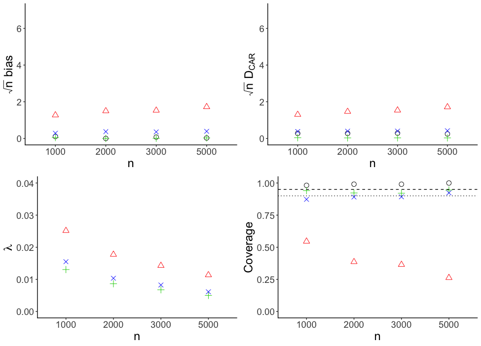
Figure 1: Comparative performance of inverse probability weighting variants in scenario 1. Circle: parametric; Triangle: nonparametric with cross-validated $\lambda$ selector; “+”: $D_{\text{CAR}}$-based $\lambda$ selector; “x”: score-based $\lambda$ selector.

Figures 1 and 2 display the results for scenarios 1 and 2, respectively. The inverse probability weighted estimators based on undersmoothing of the highly adaptive lasso outperform those based on the cross-validated highly adaptive lasso in terms of both bias and efficiency, producing similar results as the inverse probability weighted estimators based on the correctly specified parametric model for the propensity score.

The first row of each figure presents the bias and the cross-validated mean of $D_{\text{CAR}}$ (both scaled by $n^{1/2}$) of the corresponding estimators, where the latter is the objective function in equation 5, and expected to be nearly zero for estimators that solve the efficient influence function equation. While the scaled bias and the cross-validated mean of $D_{\text{CAR}}$ of the cross-validation-based selector diverges (triangle), the undersmoothed highly adaptive lasso and the correctly specified parametric models perform similarly. In terms of coverage, $D_{\text{CAR}}$-based criterion achieves the nominal coverage rate of 95%, even for smaller samples sizes, while the cross-validation-based estimator (triangle) yields a poor coverage rate of $\approx$50%. The score-based undersmoothing selectors perform reasonably well, producing inverse probability weighted estimators with coverage rates $\approx$90% for $n=1000$ and $\approx$95% at larger sample sizes ($n\geq 5000$). In scenario 2, where the parametric model of the propensity score is misspecified, the parametric inverse probability weighted estimator performs poorly, resulting in inverse probability weighted estimators with coverage rates tending to zero asymptotically. In the same scenario, the score based selector performs as well as the $D_{\text{CAR}}$-based selector producing estimators with coverage rates $\approx$95% for all the sample sizes considered. For both scenarios, we additionally report the selected tuning parameter $\lambda$ based on both the global cross-validation and undersmoothing selectors. Our results illustrate that, as sample size increases, the selected value of the tuning parameter stabilizes. Importantly, this observation implies that the undersmoothing procedure does not lead to violations of the Donsker class assumption.

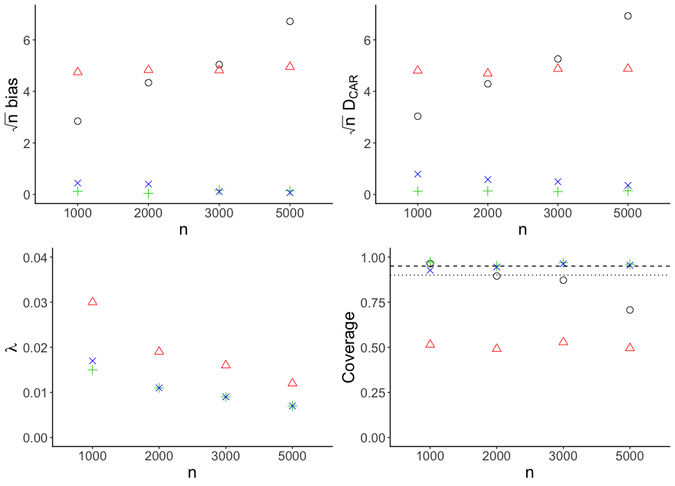
Figure 2: Performance of inverse probability weighting estimators in scenario 2. Circle: parametric; Triangle: nonparametric with cross-validated $\lambda$ selector; “+”: $D_{\text{CAR}}$-based $\lambda$ selector; “x”: score-based $\lambda$ selector.

We provide additional simulation studies in Section LABEL:supp:addl_sims of the Supplementary Material, in which we examine the relative performance of our proposed estimators under differing outcome and propensity score models, including settings corresponding to treatment randomization and observational studies with positivity violations.

6 Empirical Illustration

6.1 Overview and problem setup

We now apply our proposed estimation strategy to assessing the effect of smoking cessation on weight gain, using a subset of data from the National Health and Nutrition Examination Survey Data I Epidemiologic Follow-up Study (NHEFS). As per Hernán & Robins (2020), the NHEFS was jointly initiated by the National Center for Health Statistics and the National Institute on Aging, in collaboration with several other agencies of the United States Public Health Service. The study was designed to investigate the impact of a variety of clinical, nutritional, and behavioral factors on health outcomes including morbidity and mortality. The subset of the NHEFS data we consider totaled $n=1566$ cigarette smokers, all between the ages of 25 and 74; the data is available at https://hsph.harvard.edu/miguel-hernan/causal-inference-book. Each individual must have been present for a baseline visit and a follow-up visit roughly 10 years later. Individual weight gain was measured as a difference between baseline body weight and body weight at a follow-up visit; moreover, individuals were classified as having been in the treatment group if they reported having quit smoking prior to the follow-up visit and in the control group otherwise. Hernán & Robins (2020) caution that this subset of the NHEFS data could suffer from selection bias. As correcting for such a bias is tangent to the illustration of our analytic approach, we forego standard corrections, warning of this as a caveat of our demonstration. In practice, we advocate the use of our strategy in tandem with censoring or selection bias corrections, such as imputation or re-weighting by inverse probability of censoring (e.g., Carpenter et al., 2006; Seaman et al., 2012).

6.2 Estimation strategy

We consider estimating the average treatment effect of smoking cessation on weight gain in this subset of the NHEFS cohort ($n=1566$). A fairly rich set of baseline covariates — including sex, race, age, highest degree of formal education, intensity of smoking, years of smoking, exercise habits, indicators of an active lifestyle, and weight at study onset — were considered as potential baseline confounders of the relationship between smoking cessation and weight gain. Constructing inverse probability weighted estimators for the average treatment effect requires estimation of the propensity score, to model the conditional probability of smoking cessation given potential baseline confounders. An inverse probability weighted estimator for the average treatment effect of smoking cessation may be constructed based on distinct estimators of the respective treatment-specific means. We compare estimates of the average treatment effect based on both parametric and nonparametric strategies for estimating the propensity score, including

1. logistic regression with main terms for all baseline covariates;

2. logistic regression with main terms for all baseline covariates and with quadratic terms for age, smoking intensity, years of smoking, and baseline weight; and

3. the highly adaptive lasso with basis functions for all terms up to and including 3-way interactions between the baseline covariates, fit with $5$-fold cross-validation.

The series highly adaptive lasso of propensity score models was constructed weakening the restriction placed on the $L_{1}$-norm following an fit via global cross-validation.

6.3 Results

We apply each of the inverse probability weighted estimators to recover the average treatment effect of smoking cessation on weight gain, controlling for possible confounding by the baseline covariates previously enumerated. Table 1 summarizes the results. Generally, estimates of the average treatment effect were similar across the two classes of inverse probability weighted estimators. When the propensity score was estimated via a main terms logistic regression model, the estimate was 3.32 (CI: [2.15, 4.49]); likewise, when a logistic regression model with several quadratic terms was used, the estimate was 3.42 (CI: [2.24, 4.61]). By contrast, our cross-fitted (10 fold) nonparametric inverse probability weighted estimators based on the highly adaptive lasso produced estimates of 3.23 (CI: [2.21, 4.26]) and 3.38 (CI: [2.29, 4.48]), for the $D_{\text{CAR}}$ and score-based variants, respectively. Confidence intervals corresponding to the proposed nonparametric estimators are about 12% shorter than those obtained by the parametric estimators, due to the relatively enhanced efficiency of our estimators. Since the form of the canonical gradient is readily known for the average treatment effect, in this case, the $D_{CAR}$-based estimator provides the most reliable estimate. We note that the $D_{CAR}$-based estimate of the average treatment effect is lower in magnitude than those recovered by parametric methods, suggesting that the impact of smoking cessation on weight gain may perhaps be attenuated when the propensity score is estimated with an approach that is much less likely to be misspecified than the parametric models relied upon in standard practice.

Table 1: Estimates of the average treatment effect from inverse probability weighted estimators using propensity score models based on logistic regression and the highly adaptive lasso selected via the $D_{\text{CAR}}$ and score-based criteria.

Estimator	Lower 95% CI	Estimate	Upper 95% CI
Highly adaptive lasso ($D_{\text{CAR}}$)	2.21	3.23	4.26
Highly adaptive lasso (Score)	2.29	3.38	4.48
Logistic regression (main terms only)	2.15	3.32	4.49
Logistic regression (with quadratic terms)	2.24	3.42	4.61

References

- Bang & Robins (2005) Bang, H. & Robins, J. M. (2005). Doubly robust estimation in missing data and causal inference models. Biometrics 61, 962–973.
- Benkeser et al. (2017) Benkeser, D., Carone, M., van der Laan, M. J. & Gilbert, P. B. (2017). Doubly robust nonparametric inference on the average treatment effect. Biometrika 104, 863–880.
- Benkeser & van der Laan (2016) Benkeser, D. & van der Laan, M. J. (2016). The highly adaptive lasso estimator. In 2016 IEEE international conference on data science and advanced analytics (DSAA). IEEE.
- Bibaut & van der Laan (2019) Bibaut, A. F. & van der Laan, M. J. (2019). Fast rates for empirical risk minimization over càdlàg functions with bounded sectional variation norm. arXiv preprint arXiv:1907.09244 .
- Cao et al. (2009) Cao, W., Tsiatis, A. A. & Davidian, M. (2009). Improving efficiency and robustness of the doubly robust estimator for a population mean with incomplete data. Biometrika 96, 723–734.
- Carpenter et al. (2006) Carpenter, J. R., Kenward, M. G. & Vansteelandt, S. (2006). A comparison of multiple imputation and doubly robust estimation for analyses with missing data. Journal of the Royal Statistical Society: Series A (Statistics in Society) 169, 571–584.
- Coyle et al. (2019) Coyle, J. R., Hejazi, N. S. & van der Laan, M. J. (2019). hal9001: The scalable highly adaptive lasso. R package version 0.2.5.
- Gill et al. (1995) Gill, R. D., van der Laan, M. J. & Wellner, J. A. (1995). Inefficient estimators of the bivariate survival function for three models. In Annales de l’IHP Probabilités et statistiques, vol. 31.
- Hernán et al. (2000) Hernán, M. Á., Brumback, B. & Robins, J. M. (2000). Marginal structural models to estimate the causal effect of zidovudine on the survival of HIV-positive men. Epidemiology , 561–570.
- Hernán & Robins (2020) Hernán, M. A. & Robins, J. M. (2020). Causal Inference: What If. CRC Boca Raton, FL.
- Imbens & Rubin (2015) Imbens, G. W. & Rubin, D. B. (2015). Causal inference in statistics, social, and biomedical sciences. Cambridge University Press.
- Kang & Schafer (2007) Kang, J. D. & Schafer, J. L. (2007). Demystifying double robustness: A comparison of alternative strategies for estimating a population mean from incomplete data. Statistical science 22, 523–539.
- Klaassen (1987) Klaassen, C. A. (1987). Consistent estimation of the influence function of locally asymptotically linear estimators. The Annals of Statistics , 1548–1562.
- Pearl (2000) Pearl, J. (2000). Causality: Models, Reasoning, and Inference. Cambridge University Press, Cambridge.
- R Core Team (2020) R Core Team (2020). R: A Language and Environment for Statistical Computing. R Foundation for Statistical Computing, Vienna, Austria.
- Robins et al. (2000) Robins, J. M., Hernán, M. Á. & Brumback, B. (2000). Marginal structural models and causal inference in epidemiology.
- Robins et al. (1994) Robins, J. M., Rotnitzky, A. & Zhao, L. P. (1994). Estimation of regression coefficients when some regressors are not always observed. Journal of the American statistical Association 89, 846–866.
- Rotnitzky et al. (1998) Rotnitzky, A., Robins, J. M. & Scharfstein, D. O. (1998). Semiparametric regression for repeated outcomes with nonignorable nonresponse. Journal of the american statistical association 93, 1321–1339.
- Seaman et al. (2012) Seaman, S. R., White, I. R., Copas, A. J. & Li, L. (2012). Combining multiple imputation and inverse-probability weighting. Biometrics 68, 129–137.
- Tsiatis (2007) Tsiatis, A. (2007). Semiparametric theory and missing data. Springer Science & Business Media.
- van der Laan (2014) van der Laan, M. J. (2014). Targeted estimation of nuisance parameters to obtain valid statistical inference. The international journal of biostatistics 10, 29–57.
- van der Laan (2017) van der Laan, M. J. (2017). A generally efficient targeted minimum loss based estimator based on the highly adaptive lasso. The international journal of biostatistics 13.
- van der Laan et al. (2019) van der Laan, M. J., Benkeser, D. & Cai, W. (2019). Efficient estimation of pathwise differentiable target parameters with the undersmoothed highly adaptive lasso. arXiv preprint arXiv:1908.05607 .
- van der Laan & Bibaut (2017) van der Laan, M. J. & Bibaut, A. F. (2017). Uniform consistency of the highly adaptive lasso estimator of infinite-dimensional parameters. arXiv preprint arXiv:1709.06256 .
- van der Laan & Robins (2003) van der Laan, M. J. & Robins, J. M. (2003). Unified methods for censored longitudinal data and causality. Springer Science & Business Media.
- Vermeulen & Vansteelandt (2015) Vermeulen, K. & Vansteelandt, S. (2015). Bias-reduced doubly robust estimation. Journal of the American Statistical Association 110, 1024–1036.
- Vermeulen & Vansteelandt (2016) Vermeulen, K. & Vansteelandt, S. (2016). Data-adaptive bias-reduced doubly robust estimation. The international journal of biostatistics 12, 253–282.