Magnetic helicity in plasma of chiral fermions electroweakly interacting with inhomogeneous matter

Abstract

We study chiral fermions electroweakly interacting with a background matter having the nonuniform density and the velocity arbitrarily depending on coordinates. The dynamics of this system is described approximately by finding the Berry phase. The effective action and the kinetic equations for right and left particles are derived. In the case of a rotating matter, we obtain the correction to the anomalous electric current and to the Adler anomaly. Then we study some astrophysical applications. Assuming that the chiral imbalance in a rotating neutron star vanishes, we obtain the rate of the magnetic helicity change owing to the interaction of chiral electrons with background neutrons. The characteristic time of the helicity change turns out to coincide with the period of the magnetic cycle of some pulsars.

1 Introduction

Studies of the chiral phenomena, apart from the purely theoretical interest, find numerous applications in cosmology, astroparticle physics, accelerator and solid state physics. There is a possibility to explain the asymmetry in heavy ions collisions basing on the chiral magnetic (CME) and the chiral vortical (CVE) effects [1, 2]. The CME and the chiral separation effect (CSE) are supposed to be observed in Weyl and Dirac semimetals [3] and magnetized atomic gases [4]. The generation of cosmological magnetic fields and the lepton asymmetry can be accounted for by the CME after the electroweak phase transition [5] and for hypermagnetic fields before this phase transition [6].

The CME and CVE can be used in astrophysics mainly for the explanation of the generation of strong magnetic fields with $B>10^{15}\,\text{G}$ observed in some compact stars, known as magnetars [7]. The application of these chiral effects in the neutrino sector in connection to the magnetars problem was made in Refs. [8, 9]. The explanation of pulsars kicks basing on the anomalous hydrodynamics was proposed in Ref. [10]. The study of the magnetic fields generation in magnetars accounting for the CME in turbulent matter was carried out in Ref. [11].

We proposed various applications of the chiral phenomena for the explanation of strong magnetic fields in magnetars in Refs. [12, 13, 14, 15]. Note that both the CME and the CSE were used in Refs. [14, 15] to tackle the problem of strong magnetic fields in magnetars. In the present paper, we continue the series of our previous works for the study of the magnetic fields evolution in compact stars. Now, we analyze how the evolution of the magnetic helicity is driven by the electroweak interaction of chiral fermions with dense inhomogeneous electroweak matter inside a compact star.

In the present work, we study the plasma of ultrarelativistic electrons electrowealy interacting with nonrelativistic background matter composed of neutrons and protons. The electroweak interaction is accounted for in the Fermi approximation. The characteristics of this matter, such as the density and the macroscopic velocity can depend on coordinates. The electron gas is supposed to be degenerate, with the Fermi momentum $p_{\mathrm{F}e}$ being much greater than the electron mass $m_{e}$. Such a system may well exist in a neutron star (NS). The application of the chiral phenomena to electrons is justified since these particles are ultrarelativistic: $p_{\mathrm{F}e}\gg m_{e}$. Anomalous electric currents of protons are negligible since protons are nonrelativistic in NS. Hydrodynamic currents of neutrinos, which are ultrarelativistic particles, can receive an anomalous contribution. However, the fluxes of neutrinos are small for an old NS, studied in our work. Thus, we neglect the neutrino contribution.

This work is organized in the following way. First, in Sec. 2, we formulate the dynamics of chiral fermions in dense inhomogeneous matter, with the electroweak interaction being accounted for. The evolution of chiral fermions was described approximately basing on the Berry phase evolution. We find the effective actions and the kinetic equations for chiral fermions in Sec. 2. Then, in Sec. 3, we derive the corrections to the anomalous electric current and to the Adler anomaly from the electroweak interaction with inhomogeneous matter. Finally, we apply our results in Sec. 4 for the description of the magnetic helicity evolution in a rotating NS and compare our prediction for the period of the magnetic cycle with the astronomical observations. We conclude in Sec. 5.

2 Approximate description of chiral plasma based on the Berry phase evolution

We start with the consideration of a chiral fermion motion in electroweak background matter. The interaction with the electromagnetic field will be accounted for later. The Dirac equation for such a fermion, which is an electron, reads,

$$\mathrm{i}\dot{\psi}=\left[(\bm{\alpha}\hat{\mathbf{p}})+V_{\mathrm{R}}^{\mu}\gamma^{0}\gamma_{\mu}P_{\mathrm{R}}+V_{\mathrm{L}}^{\mu}\gamma^{0}\gamma_{\mu}P_{\mathrm{L}}\right]\psi,$$ (1)

where $\hat{\mathbf{p}}=-\mathrm{i}\nabla$ is the momentum operator, $\psi$ is the bispinor of the fermion, $\gamma^{\mu}=(\gamma^{0},\bm{\gamma})$, $\bm{\alpha}=\gamma^{0}\bm{\gamma}$, and $\gamma^{5}=\mathrm{i}\gamma^{0}\gamma^{1}\gamma^{2}\gamma^{3}$ are the Dirac matrices, $P_{\mathrm{R,L}}=(1\pm\gamma^{5})/2$ are the chiral projectors, and $V_{\mathrm{R},\mathrm{L}}^{\mu}=V_{\mathrm{R},\mathrm{L}}^{\mu}(\mathbf{x})=(V_{\mathrm{R},\mathrm{L}}^{0},\mathbf{V}_{\mathrm{R,L}})$ are the effective potentials for the interaction of the chiral projections with inhomogeneous matter. The explicit expressions for $V_{\mathrm{R},\mathrm{L}}^{0}\sim G_{\mathrm{F}}n_{f}$ for electrons can be found in Ref. [12]. Here $n_{f}$ is the density of background particles and $G_{\mathrm{F}}=1.17\times 10^{-5}\,\text{GeV}^{-2}$ is the Fermi constant. If we consider arbitrarily moving unpolarized background matter, then $\mathbf{V}_{\mathrm{R},\mathrm{L}}=V_{\mathrm{R},\mathrm{L}}^{0}\mathbf{v}$ [16], where $\mathbf{v}(\mathbf{x})$ is the velocity of plasma, in which all background particles are supposed to move as a whole. The density of background matter can be also the function of coordinates, $n_{f}=n_{f}(\mathbf{x})$. Note that $V_{\mathrm{R}}^{\mu}\neq V_{\mathrm{L}}^{\mu}$ since the electroweak interaction violates parity.

Using the chiral representation for the Dirac matrices, we can rewrite $\psi$ in the form of two chiral projections, $\psi^{\mathrm{T}}=(\psi_{\mathrm{R}},\psi_{\mathrm{L}})$. Basing on Eq. (1), one gets the wave equations for $\psi_{\mathrm{R,L}}$,

$$\mathrm{i}\dot{\psi}_{\mathrm{R,L}}=\left[\pm(\bm{\sigma}\hat{\mathbf{p}})+V_{\mathrm{R,L}}^{0}\mp(\bm{\sigma}\mathbf{V}_{\mathrm{R,L}})\right]\psi_{\mathrm{R,L}},$$ (2)

where $\bm{\sigma}$ are the Pauli matrices.

The solution of Eq. (2) for the arbitrary dependence $V_{\mathrm{R},\mathrm{L}}^{\mu}(\mathbf{x})$ is barely possible. However, we can analyze the evolution of $\psi_{\mathrm{R,L}}$ quasiclassically using the concept of the Berry phase [17]. For this purpose we shift from the field theory to the classical mechanics, i.e. we take that particles move along some trajectories. Thus we should appropriately introduce the canonical coordinates $\{\mathbf{x}(t),\mathbf{p}(t)\}$. In principle, the choice of the coordinates is voluntary. Therefore, instead of the wave functions $\psi_{\mathrm{R,L}}(\mathbf{x},t)$, depending on time $t$ and the coordinates $\mathbf{x}$, we consider the dependence on $t$ only, $\psi_{\mathrm{R,L}}(t)$: $\psi_{\mathrm{R,L}}(\mathbf{x},t)\to\exp(\mathrm{i}\Phi)\psi_{\mathrm{R,L}}(t)$, where $\Phi=\Phi(\mathbf{x},\mathbf{p})$ is the phase which depends on the canonical coordinates. We do not fix the form of $\Phi$ yet.

Using Eq. (2), we get that the time dependent spinors $\psi_{\mathrm{R,L}}=\psi_{\mathrm{R,L}}(t)$ evolve as

$$\mathrm{i}\dot{\psi}_{\mathrm{R,L}}=H_{\mathrm{R,L}}\psi_{\mathrm{R,L}},\quad H_{\mathrm{R,L}}=\pm(\bm{\sigma}\bm{\Pi})+V_{\mathrm{R,L}}^{0},$$ (3)

where $\bm{\Pi}=\nabla\Phi-\mathbf{V}_{\mathrm{R,L}}$. The Hamiltonians $H_{\mathrm{R,L}}$ in Eq. (3) depend on $t$ only since particles move along the trajectories $\mathbf{x}=\mathbf{x}(t)$.

Now we assume the adiabatic change of $H_{\mathrm{R,L}}$. In this case, we take that [18]

$$\psi_{\mathrm{R,L}}(t)=\exp(-\mathrm{i}\Theta_{\mathrm{R,L}})u_{\mathrm{R,L}},$$ (4)

where $\Theta_{\mathrm{R,L}}=\Theta_{\mathrm{R,L}}(t)$ is the Berry phase [17], which is different for right and left particles, and $u_{\mathrm{R,L}}$ are the constant spinors. We impose the following constraints on $\psi_{\mathrm{R,L}}$ [18]:

$$\psi_{\mathrm{R,L}}^{\dagger}\psi_{\mathrm{R,L}}=1,\quad\psi_{\mathrm{R,L}}^{\dagger}\dot{\psi}_{\mathrm{R,L}}=0,$$ (5)

to fix their amplitudes and the phases.

To find $\Theta_{\mathrm{R,L}}$, first, we solve the Schrödinger equation [18],

$$E_{\mathrm{R,L}}u_{\mathrm{R,L}}(\xi)=H_{\mathrm{R,L}}u_{\mathrm{R,L}}(\xi),$$ (6)

in which the canonical variable $\xi_{a}=\{\mathbf{x},\mathbf{p}\}$, $a=1,\dots,6$, is supposed to be constant: $\xi_{a}=\text{const}$. The solution has the form,

$$E_{\mathrm{R,L}}=V_{\mathrm{R,L}}^{0}+|\bm{\Pi}|,\quad u_{\mathrm{R}}=\left(\begin{array}[]{c}e^{-\mathrm{i}\varphi/2}\cos\dfrac{\theta}{2}\\ e^{\mathrm{i}\varphi/2}\sin\dfrac{\theta}{2}\end{array}\right),\quad u_{\mathrm{L}}=\left(\begin{array}[]{c}-e^{-\mathrm{i}\varphi/2}\sin\dfrac{\theta}{2}\\ e^{\mathrm{i}\varphi/2}\cos\dfrac{\theta}{2}\end{array}\right),$$ (7)

where the angles $\varphi$ and $\theta$ fix the direction of the vector $\bm{\Pi}$.

Using Eqs. (3)-(6), we get that the Berry phases $\Theta_{\mathrm{R,L}}$ obey the equation [18],

$$\mathrm{i}\dot{\Theta}_{\mathrm{R,L}}=u_{\mathrm{R,L}}^{\dagger}\frac{\partial u_{\mathrm{R,L}}}{\partial\xi_{a}}\dot{\xi}_{a}.$$ (8)

The solution of Eq. (8) reads [18]

$$\Theta_{\mathrm{R,L}}(t)=\int_{C}A_{a}^{(\mathrm{R,L})}(\xi)\mathrm{d}\xi_{a},$$ (9)

where $C$ is the particle trajectory in the phase space and

$$A_{a}^{(\mathrm{R,L})}=-\mathrm{i}u_{\mathrm{R,L}}^{\dagger}\frac{\partial u_{\mathrm{R,L}}}{\partial\xi_{a}},$$ (10)

is the Berry connection [18].

It is convenient to represent the Berry connection in terms of two three-dimensional vectors, $A_{a}^{(\mathrm{R,L})}=(\bm{\mathcal{B}}_{\mathrm{R,L}},\bm{\mathcal{A}}_{\mathrm{R,L}})$. Then, using Eq. (10), we obtain that

$$\mathcal{A}_{i}^{(\mathrm{R,L})} =-\mathrm{i}u_{\mathrm{R,L}}^{\dagger}\frac{\partial u_{\mathrm{R,L}}}{\partial p_{i}}=-\mathrm{i}u_{\mathrm{R,L}}^{\dagger}\frac{\partial u_{\mathrm{R,L}}}{\partial\Pi_{j}}\frac{\partial\Pi_{j}}{\partial p_{i}},$$

$$\mathcal{B}_{i}^{(\mathrm{R,L})} =-\mathrm{i}u_{\mathrm{R,L}}^{\dagger}\frac{\partial u_{\mathrm{R,L}}}{\partial x_{i}}=-\mathrm{i}u_{\mathrm{R,L}}^{\dagger}\frac{\partial u_{\mathrm{R,L}}}{\partial\Pi_{j}}\frac{\partial\Pi_{j}}{\partial x_{i}}.$$ (11)

Therefore, instead of the integration along the particle trajectory, we can rewrite Eq. (9) in the form,

$$\Theta_{\mathrm{R,L}}(t)=\int_{t_{0}}^{t}\left(\bm{\mathcal{B}}_{\mathrm{R,L}}\dot{\mathbf{x}}+\bm{\mathcal{A}}_{\mathrm{R,L}}\dot{\mathbf{p}}\right)\mathrm{d}t=\int_{t_{0}}^{t}\mathcal{A}_{\bm{\Pi}j}^{(\mathrm{R,L})}\left[\frac{\partial\Pi_{j}}{\partial p_{i}}\dot{p}_{i}+\frac{\partial\Pi_{j}}{\partial x_{i}}\dot{x}_{i}\right]\mathrm{d}t,$$ (12)

where

$$\mathcal{A}_{\bm{\Pi}j}^{(\mathrm{R,L})}=-\mathrm{i}u_{\mathrm{R,L}}^{\dagger}\frac{\partial u_{\mathrm{R,L}}}{\partial\Pi_{j}},$$ (13)

which results from Eq. (2).

The wave function evolves as $\psi_{\mathrm{R,L}}(t)\sim\exp(-\mathrm{i}\Theta_{\mathrm{R,L}})$ in Eq. (4). Recalling that the spinors $u_{\mathrm{R,L}}$ have the energies $E_{\mathrm{R,L}}$ in Eq. (7) and accounting for Eq. (12), we can define the effective energies,

$$E_{\mathrm{eff}}=E_{\mathrm{R,L}}+\mathcal{A}_{\bm{\Pi}j}^{(\mathrm{R,L})}\left[\frac{\partial\Pi_{j}}{\partial p_{i}}\dot{p}_{i}+\frac{\partial\Pi_{j}}{\partial x_{i}}\dot{x}_{i}\right].$$ (14)

Now we suppose that chiral fermions have the electric charge $e$ and interact with the external electromagnetic field $A^{\mu}=(A_{0},\mathbf{A})$. Accounting for Eq. (14), we obtain the effective actions for such particles,

$$S_{\mathrm{eff}}^{(\mathrm{R,L})}[\mathbf{x},\mathbf{p}]= \int_{t_{0}}^{t}\mathrm{d}t\bigg{\{}\dot{\mathbf{x}}\left[\mathbf{p}+e\mathbf{A}(\mathbf{x})\right]-\mathcal{A}_{\bm{\Pi}j}^{(\mathrm{R,L})}\left[\frac{\partial\Pi_{j}}{\partial p_{i}}\dot{p}_{i}+\frac{\partial\Pi_{j}}{\partial x_{i}}\dot{x}_{i}\right]$$

$$-\epsilon_{\mathrm{R,L}}(\mathbf{x})-eA_{0}(\mathbf{x})\bigg{\}},$$ (15)

where, following Ref. [19], we introduce the particle energy dependence on coordinates $\epsilon_{\mathrm{R,L}}(\mathbf{x})$.

Up to now, the canonical coordinates and, hence $\bm{\Pi}$, are not specified. We can choose $\{\mathbf{x},\mathbf{p}\}$ in such a way that $\Phi=(\mathbf{px})$. In this case,

$$\bm{\Pi}\equiv\mathbf{P}=\mathbf{p}-\mathbf{V}_{\mathrm{R,L}},\quad\frac{\partial\Pi_{j}}{\partial p_{i}}=\delta_{ij},\quad\frac{\partial\Pi_{j}}{\partial x_{i}}=-\frac{\partial V_{j}^{(\mathrm{R,L})}}{\partial x_{i}},$$ (16)

and $\epsilon_{\mathbf{P}}^{(\mathrm{R,L})}(\mathbf{x})=V_{\mathrm{R,L}}^{0}+|\mathbf{P}|+\epsilon_{0}$, where $\epsilon_{0}=\epsilon_{0}(\mathbf{x})$ arises owing to the possible dependence of the electromagnetic field on coordinates.

The effective action in Eq. (2) takes the form,

$$S_{\mathrm{eff}}^{(\mathrm{R,L})}=\int_{t_{0}}^{t}\mathrm{d}t\left\{\dot{\mathbf{x}}\left[\mathbf{p}+e\mathbf{A}(\mathbf{x})\right]-\bm{\mathcal{A}}_{\mathrm{R,L}}\left[\dot{\mathbf{p}}-(\dot{\mathbf{x}}\nabla)\mathbf{V}_{\mathrm{R,L}}\right]-\epsilon_{\mathbf{P}}^{(\mathrm{R,L})}(\mathbf{x})-eA_{0}(\mathbf{x})\right\},$$ (17)

where, for brevity, we omit the index $\mathbf{P}$ in the Berry connection: $\bm{\mathcal{A}}_{\mathbf{P}}^{(\mathrm{R,L})}\to\bm{\mathcal{A}}_{\mathrm{R,L}}$. Using the fact that $\dot{\mathbf{P}}=\dot{\mathbf{p}}-(\dot{\mathbf{x}}\nabla)\mathbf{V}_{\mathrm{R,L}}$, we can rewrite Eq. (17) as

$$S_{\mathrm{eff}}^{(\mathrm{R,L})}[\mathbf{x},\mathbf{P}]=\int_{t_{0}}^{t}\mathrm{d}t\left\{\dot{\mathbf{x}}\left[\mathbf{P}+e\mathbf{A}_{\mathrm{eff}}(\mathbf{x})\right]-\bm{\mathcal{A}}_{\mathrm{R,L}}\dot{\mathbf{P}}-\epsilon_{\mathbf{P}}^{(\mathrm{R,L})}(\mathbf{x})-eA_{0}(\mathbf{x})\right\},$$ (18)

where $\mathbf{A}_{\mathrm{eff}}=\mathbf{A}+\mathbf{V}_{\mathrm{R,L}}/e$. Now we can use the canonical variables $\Xi_{a}=\{\mathbf{x},\mathbf{P}\}$. This choice of canonical variables to construct a kinetic equation of a fermion, electroweakly interacting with inhomogeneous background matter, coincides with that in Ref. [20]. One just needs to replace $\mathbf{p}\leftrightarrow\mathbf{P}$ in Ref. [20].

Basing on Eq. (18) and applying the approach developed in Ref. [19], we obtain the kinetic equation for the distribution functions $f_{\mathrm{R,L}}(\mathbf{x},\mathbf{P},t)$ of right and left fermions in the form,

$$\frac{\partial f_{\mathrm{R,L}}}{\partial t}+ \frac{1}{1+e\mathbf{B}_{\mathrm{eff}}\bm{\Omega}}\bigg{\{}\left[\mathbf{v}+e(\tilde{\mathbf{E}}\times\bm{\Omega}_{\mathbf{P}})+e(\mathbf{v}\cdot\bm{\Omega}_{\mathbf{P}})\mathbf{B}_{\mathrm{eff}}\right]\frac{\partial f_{\mathrm{R,L}}}{\partial\mathbf{x}}$$

$$+\left[e\tilde{\mathbf{E}}+e(\mathbf{v}\times\mathbf{B}_{\mathrm{eff}})+e^{2}(\tilde{\mathbf{E}}\cdot\mathbf{B}_{\mathrm{eff}})\bm{\Omega}_{\mathbf{P}}\right]\frac{\partial f_{\mathrm{R,L}}}{\partial\mathbf{P}}\bigg{\}}=0,$$ (19)

where $\tilde{\mathbf{E}}=\mathbf{E}_{\mathrm{eff}}-e^{-1}\partial\epsilon_{\mathbf{P}}/\partial\mathbf{x}$, $\mathbf{v}=\partial\epsilon_{\mathbf{P}}/\partial\mathbf{P}$, $\mathbf{E}_{\mathrm{eff}}=-\nabla A_{0}-\nabla V_{\mathrm{R,L}}^{0}/e$, $\mathbf{B}_{\mathrm{eff}}=(\nabla\times\mathbf{A}_{\mathrm{eff}})$, and $\bm{\Omega}_{\mathbf{P}}=(\nabla_{\mathbf{P}}\times\bm{\mathcal{A}}_{\mathrm{R,L}})$ is the Berry curvature. To derive Eq. (2) we take $\epsilon_{\mathbf{P}}^{(\mathrm{R,L})}=V_{\mathrm{R,L}}^{0}+\epsilon_{\mathbf{P}}$, where $\epsilon_{\mathbf{P}}(\mathbf{x})=|\mathbf{P}|+\epsilon_{0}(\mathbf{x})$.

Note that, if $\epsilon_{0}(\mathbf{x})=0$, Eq. (2) coincides with that derived in Refs. [21, 22] for a neutrino electroweakly interacting with electron-positron plasma since $\tilde{\mathbf{E}}=\mathbf{E}_{\mathrm{eff}}=\mathbf{E}+\mathbf{E}_{\mathrm{EW}}$ and $\mathbf{B}_{\mathrm{eff}}=\mathbf{B}+\mathbf{B}_{\mathrm{EW}}$, where $\mathbf{E}_{\mathrm{EW}}=-e^{-1}\nabla V_{\mathrm{R,L}}^{0}$ and $\mathbf{B}_{\mathrm{EW}}=e^{-1}(\nabla\times\mathbf{V}_{\mathrm{R,L}})$ are the effective corrections induced by the electroweak interaction to the conventional electromagnetic field $F_{\mu\nu}=(\mathbf{E},\mathbf{B})$.

3 Electric current and Adler anomaly in inhomogeneous matter accounting for the electroweak interaction

In this section, we derive the corrections to the anomalous current and to the Adler anomaly arising from the electroweak interaction of chiral fermions with inhomogeneous background matter. We consider the particular case of the rotating matter.

Defining the currents [19]

$$\mathbf{j}_{\mathrm{R,L}}= -\int\frac{\mathrm{d}^{3}P}{(2\pi)^{3}}\bigg{[}\epsilon_{\mathbf{P}}\frac{\partial f_{\mathrm{R,L}}}{\partial\mathbf{P}}+e\left(\bm{\Omega}_{\mathbf{P}}\cdot\frac{\partial f_{\mathrm{R,L}}}{\partial\mathbf{P}}\right)\epsilon_{\mathbf{P}}\mathbf{B}_{\mathrm{eff}}$$

$$+\epsilon_{\mathbf{P}}\left(\bm{\Omega}_{\mathbf{P}}\times\frac{\partial f_{\mathrm{R,L}}}{\partial\mathbf{x}}\right)+e\left(\mathbf{E}_{\mathrm{eff}}\times\bm{\Omega}_{\mathbf{P}}\right)f_{\mathrm{R,L}}\bigg{]},$$ (20)

and the number densities [19]

$$n_{\mathrm{R,L}}=\int\frac{\mathrm{d}^{3}P}{(2\pi)^{3}}\left[1+e\left(\mathbf{B}_{\mathrm{eff}}\cdot\bm{\Omega}_{\mathbf{P}}\right)\right]f_{\mathrm{R,L}}$$ (21)

one gets that these quantities obey the equation [21, 22],

$$\partial_{t}n_{\mathrm{R,L}}+(\nabla\cdot\mathbf{j}_{\mathrm{R,L}})=-e^{2}\int\frac{\mathrm{d}^{3}P}{(2\pi)^{3}}\left(\bm{\Omega}_{\mathbf{P}}\cdot\frac{\partial f_{\mathrm{R,L}}}{\partial\mathbf{P}}\right)\left(\mathbf{E}_{\mathrm{eff}}\cdot\mathbf{B}_{\mathrm{eff}}\right).$$ (22)

The derivation of Eq. (5) implies the validity of the Maxwell equations for the effective electromagnetic fields [21, 22]: $(\nabla\cdot\mathbf{B}_{\mathrm{eff}})=0$ and $\partial_{t}\mathbf{B}_{\mathrm{eff}}+(\nabla\times\mathbf{E}_{\mathrm{eff}})=0$.

Let us suppose that the distribution functions are homogeneous: $\partial f_{\mathrm{R,L}}/\partial\mathbf{x}=0$. In this case, $\epsilon_{\mathbf{P}}=\mu_{\mathrm{R,L}}+\dotsb$, where $\mu_{\mathrm{R,L}}$ are the chemical potentials of right and left fermions and we keep only the zero order terms in the Fermi constant $G_{\mathrm{F}}$. We obtain that the anomalous part of the electric current $\mathbf{J}_{\mathrm{R,L}}=e\mathbf{j}_{\mathrm{R,L}}$ can be expressed in the following way:

$$\mathbf{J}_{\mathrm{R,L}}= -\mu_{\mathrm{R,L}}e^{2}\mathbf{B}_{\mathrm{eff}}\int\frac{\mathrm{d}^{3}P}{(2\pi)^{3}}\left(\bm{\Omega}_{\mathbf{P}}\cdot\frac{\partial f_{\mathrm{R,L}}}{\partial\mathbf{P}}\right)=\pm\frac{e^{2}}{4\pi^{2}}\mu_{\mathrm{R,L}}\mathbf{B}_{\mathrm{eff}}$$

$$=\pm\frac{e^{2}}{4\pi^{2}}\mu_{\mathrm{R,L}}\left[\mathbf{B}+\frac{1}{e}(\nabla\times\mathbf{V}_{\mathrm{R,L}})\right].$$ (23)

The first term in Eq. (3), $\mathbf{J}_{\mathrm{R,L}}\parallel\mu_{\mathrm{R,L}}\mathbf{B}$, is the well known CME [23]. To derive Eq. (3) we take the distribution function in the form,

$$f_{\mathrm{R,L}}(\mathbf{P})=\left\{\exp[\beta(|\mathbf{P}|-\mu_{\mathrm{R,L}})]+1\right\}^{-1},\quad\frac{\partial f_{\mathrm{R,L}}}{\partial\mathbf{P}}=-\frac{\mathbf{P}}{|\mathbf{P}|}\frac{\beta\exp[\beta(|\mathbf{P}|-\mu_{\mathrm{R,L}})]}{\left\{\exp[\beta(|\mathbf{P}|-\mu_{\mathrm{R,L}})]+1\right\}^{2}}.$$ (24)

where $\beta=1/T$ is the reciprocal temperature. In Eqs. (3) and (24), we consider the degenerate plasma with $\beta\to\infty$ and $\nabla_{\mathbf{P}}f_{\mathrm{R,L}}\to\delta(|\mathbf{P}|-\mu_{\mathrm{R,L}})$ and take into account that $\bm{\Omega}_{\mathbf{P}}=\pm\mathbf{P}/2|\mathbf{P}|^{3}$ [21].

Analogously Eq. (3) we can calculate the correction to the Adler anomaly using Eq. (22). First, we suppose that the number density of background matter is homogeneous, i.e. $\nabla V_{\mathrm{R,L}}^{0}=0$. In this case, $\mathbf{E}_{\mathrm{eff}}=\mathbf{E}$, and

$$\partial_{t}n_{\mathrm{R,L}}+(\nabla\cdot\mathbf{j}_{\mathrm{R,L}})=\pm\frac{e^{2}}{4\pi^{2}}\left(\mathbf{E}\cdot\mathbf{B}_{\mathrm{eff}}\right)=\pm\frac{e^{2}}{4\pi^{2}}\left[\left(\mathbf{E}\cdot\mathbf{B}\right)+\frac{1}{e}\left(\mathbf{E}\cdot\nabla\times\mathbf{V}_{\mathrm{R,L}}\right)\right].$$ (25)

Integrating this expression over the volume $V$ and neglecting the boundary effects, we obtain that

$$\frac{\mathrm{d}n_{5}}{\mathrm{d}t}=\frac{e^{2}}{2\pi^{2}V}\int\left[\left(\mathbf{E}\cdot\mathbf{B}\right)-\frac{1}{e}\left(\mathbf{E}\cdot\nabla\times\mathbf{V}_{5}\right)\right]\mathrm{d}^{3}x-\Gamma n_{5},$$ (26)

where $n_{5}=n_{\mathrm{R}}-n_{\mathrm{L}}$ is the chiral imbalance and $\mathbf{V}_{5}=(\mathbf{V}_{\mathrm{L}}-\mathbf{V}_{\mathrm{R}})/2$. We have $(\nabla\times\mathbf{V}_{5})=V_{5}\bm{\omega}$, where $V_{5}=(V_{\mathrm{L}}^{0}-V_{\mathrm{R}}^{0})/2$ and $\bm{\omega}$ is the angular velocity.

In Eq. (26), we account for the fact that electrons are ultrarelativistic but not massless particles. Hence their helicity can be changed in collisions in plasma. Thus we introduce the term $-\Gamma n_{5}$ in the right hand side of Eq. (26). The spin flip rate $\Gamma\sim 10^{11}\,\text{s}^{-1}$ was computed for an old NS in Ref. [24].

The electroweak correction to the anomalous current $\delta\mathbf{J}_{\mathrm{anom}}=(\mathbf{J}_{\mathrm{R}}+\mathbf{J}_{\mathrm{L}})\parallel\nabla\times(\mathbf{V}_{\mathrm{R}}-\mathbf{V}_{\mathrm{L}})\sim V_{5}\bm{\omega}$ in Eq. (3), in fact, reproduces the result of Ref. [25], except the factor $1/2\pi$ which was missed in Ref. [25] because of the incorrect normalization of the spinors there. The generation of such a current was named the galvano-rotational effect in Ref. [25].

4 Astrophysical applications

Let us consider the application of Eq. (26) in an astrophysical plasma. We mentioned in Sec. 3 that the spin flip rate is huge in NS. Hence, $\dot{n}_{5}\to 0$ in Eq. (26). Using Eq. (26), we get that the chiral imbalance reaches the saturated value,

$$n_{5}\to n_{5}^{(\text{sat})}=\frac{e^{2}}{2\pi^{2}V\Gamma}\int\left[\left(\mathbf{E}\cdot\mathbf{B}\right)-\frac{1}{e}\left(\mathbf{E}\cdot\nabla\times\mathbf{V}_{5}\right)\right]\mathrm{d}^{3}x,$$ (27)

We will show below that we can neglect $n_{5}^{(\text{sat})}$ in an old NS. Thus, the saturated densities of right and left electrons are equal.

If both $n_{5}$ and $\dot{n}_{5}$ are vanishing in Eq. (26), then, accounting for the fact that

$$\frac{\mathrm{d}H}{\mathrm{d}t}=-2\int\left(\mathbf{E}\cdot\mathbf{B}\right)\mathrm{d}^{3}x,$$ (28)

where

$$H=\int\left(\mathbf{A}\cdot\mathbf{B}\right)\mathrm{d}^{3}x,$$ (29)

is the magnetic helicity, we get the contribution of the electroweak interaction to the magnetic helicity evolution in the form,

$$\left(\frac{\mathrm{d}H}{\mathrm{d}t}\right)_{\mathrm{EW}}=-2\frac{V_{5}}{e}\int\left(\mathbf{E}\cdot\bm{\omega}\right)\mathrm{d}^{3}x=-2\frac{V_{5}}{e\sigma}\int\left(\nabla\times\mathbf{B}\cdot\bm{\omega}\right)\mathrm{d}^{3}x.$$ (30)

Here we take into account the Maxwell equations and the fact that $\mathbf{E}=\mathbf{J}/\sigma=(\nabla\times\mathbf{B})/\sigma$, where $\mathbf{J}$ is the ohmic current and $\sigma$ is the electric conductivity.

Equation (30) should be added to the contribution of the classical electrodynamics for the magnetic helicity evolution [26],

$$\left(\frac{\mathrm{d}H}{\mathrm{d}t}\right)_{\mathrm{class}}=-\frac{2}{\sigma}\int\left(\mathbf{J}\cdot\mathbf{B}\right)\mathrm{d}^{3}x+2\oint\left[(\mathbf{B}\cdot\mathbf{A})(\mathbf{v}\cdot\mathbf{n})-(\mathbf{v}\cdot\mathbf{A})(\mathbf{B}\cdot\mathbf{n})\right]\mathrm{d}^{2}S,$$ (31)

where $\mathbf{n}$ is the external normal to the stellar surface. The total rate of the helicity change is $\dot{H}=(\dot{H})_{\mathrm{class}}+(\dot{H})_{\mathrm{EW}}$, where the classical electrodynamics and the electroweak contributions are given in Eqs. (31) and (30) respectively. Since we concentrate mainly on the $(\dot{H})_{\mathrm{EW}}$ term in our work, we omit the subscript EW in the following.

Equation (30) describes the new mechanism for the helicity evolution owing to the electroweak interaction of chiral fermions with inhomogeneous background matter. The inhomogeneity of the interaction of chiral fermions is in the dependence of $\mathbf{V}_{\mathrm{R,L}}=V_{\mathrm{R,L}}^{0}\mathbf{v}$ on coordinates, which can take place if we consider rotating matter with the velocity $\mathbf{v}(\mathbf{x})=\bm{\omega}\times\mathbf{x}$. The anomalous contribution to the helicity evolution in Eq. (30) occurs if $(\nabla\times\mathbf{B})\parallel\bm{\omega}$. Such a situation can happen in a rotating star having a toroidal component of the magnetic field. It should be noted that the influence of quantum effects on the magnetic helicity evolution, analogous to that in Eq. (30), was studied in Ref. [27].

We suppose that a compact star has the dipole configuration of the magnetic field: the poloidal component $\mathbf{B}_{p}$ and two tori of the toriodal field $\mathbf{B}_{t}$ with different directions in the opposite hemispheres, as schematically shown in Fig. 1. Note that a stellar magnetic field having only either a poloidal or a toroidal component is unstable [28].

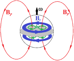
Figure 1: The schematic illustration of the stellar magnetic field configuration. The poloidal magnetic field $\mathbf{B}_{p}$, which can exist outside the star, is shown by red lines. The toroidal field $\mathbf{B}_{t}$ is concentrated within two blue tori with opposite directions above and below the stellar equator, filled by the grey color. The fluctuations of the magnetic field in the form of green rings can exist in both the northern and southern hemispheres. The direction of the magnetic field $\mathbf{b}$ in these rings coincides with that for $\mathbf{B}_{t}$.

Let us assume that the toroidal magnetic field in one of the hemispheres of the star is a source of magnetic field vortices or rings, which disattach from the torus. It can happen because of turbulence processes taking place inside some compact rotating stars [29]. Such vortices are depicted in Fig. 1 in green. It should be noted that the direction of the magnetic field in a vortex coincides with that in a torus, in which $\mathbf{B}_{t}$ is concentrated. Then, the electroweak mechanism, present in Eq. 30, acts on these vortices. The described process results in the change of the stellar magnetic field. Namely, it leads to the helicity flux through the stellar equator. Indeed, $\dot{H}$ has different signs in opposite hemispheres since $\mathbf{B}_{t}$, as well as vortices, has opposite directions in the northern and southern hemispheres. It means that $\dot{H}_{\mathrm{tot}}=\dot{H}_{\mathrm{N}}+\dot{H}_{\mathrm{S}}=0$, there $H_{\mathrm{N,S}}$ are the helicities of the northern and southern hemispheres.

We suppose that the average strength of the field in a vortex is $\mathbf{b}$ and the average width of a flux tube of a vortex is $r$. Then, assuming the hypothetical situation that all the magnetic field in the northern hemisphere transforms into vortices and accounting for the magnetic flux conservation, one gets that $br^{2}N=B_{t}R_{t}^{2}$, where $N$ is the total number of vortices and $R_{t}$ is the radius of a torus. Thus, we can estimate $(\nabla\times\mathbf{B})$ in Eq. (30) as

$$(\nabla\times\mathbf{B})\sim N\frac{b}{r}\sim\frac{B_{t}R_{t}^{2}}{r^{3}}.$$ (32)

We consider, e.g., the northern hemisphere. Then, basing on Eq. (30), we have the helicity change rate in the form,

$$\dot{H}_{\mathrm{N}}\sim-\frac{4}{3}\pi B_{t}R_{t}^{2}\omega\frac{V_{5}}{e\sigma}\frac{R^{3}}{r^{3}},$$ (33)

where $R\sim 10\,\text{km}$ is the NS radius. The typical time of the helicity change in this hemisphere is

$$\tau\sim\frac{H_{\mathrm{N}}}{|\dot{H}_{\mathrm{N}}|}=\frac{3}{4\pi}\frac{eB_{p}\sigma r^{3}}{\omega V_{5}R},$$ (34)

where we use the definition of the helicity alternative to that in Eq. (29) [30], $H=2L\Phi_{1}\Phi_{2}$, where $\Phi_{1,2}$ are the linked magnetic fluxes and $L=0,\pm 1,\dotsc$ is the linkage number. Thus, in Eq. (34), we take that $H_{\mathrm{N}}\sim B_{t}R_{t}^{2}B_{p}R^{2}$ is the total helicity in the northern hemisphere.

We consider the helicity change, proposed above, inside NS. In this case, $V_{5}=G_{\mathrm{F}}n_{n}/2\sqrt{2}=6\,\text{eV}$ [12], where $n_{n}=1.8\times 10^{38}\,\text{cm}^{-3}$ is the neutron density in NS. The application of the chiral phenomena for electrons in dense matter of NS is justified since their Fermi momentum $p_{\mathrm{F}e}=(3\pi^{2}n_{e})^{1/3}\sim 10^{2}\,\text{MeV}$ is much greater than the electron mass. Hence electrons are ultrarelativistic. Here we take that the electron density $n_{e}$ in NS is about 5% of $n_{n}$.

Then we take that $B_{p}=10^{12}\,\text{G}$ is the typical pulsar magnetic field, $\omega=10^{3}\,\text{s}^{-1}$ is the angular velocity of a millisecond pulsar, and $\sigma=10^{6}\,\text{GeV}$ is the electric conductivity of the NS matter having the temperature $T\sim 10^{7}\,\text{K}$ [31]. The magnetic flux tubes with $r\sim 6\times 10^{-5}\,\text{cm}$ were predicted in Ref. [32] to exist in matter of some NSs. Using the above values in Eq. (34), we get that $\tau=1.3\times 10^{11}\,\text{s}=4\times 10^{3}\,\text{yr}$.

In fact, we predict the magnetic helicity flux through the equator driven by the electroweak interaction of chiral electrons with the rotating matter of NS. The helicity flux through the stellar equator was found in Ref. [33] to be closely related to the cyclic variation of the magnetic field in a star. For example, it is the well known solar cycle with the period of $22\,\text{yr}$. Thus we can conclude that $\tau\sim 10^{3}\,\text{yr}$ is associated with a periodic variation of the magnetic field in NSs. It should be noted that such a cycle in NSs with $10^{2}\,\text{yr}<\tau<10^{4}\,\text{yr}$ was observed in Ref. [34] by studying the spin-down of pulsars. The mechanism proposed in our work is a possible explanation of the results of Ref. [34].

At the end of this section, we demonstrate that we can neglect $n_{5}^{(\text{sat})}$ in Eq. (27). We mentioned above that the total helicity of NS is constant. The second term in the integrand in Eq. (27), $\sim\left(\mathbf{E}\cdot\nabla\times\mathbf{V}_{5}\right)$, becomes important when turbulent rings of the magnetic field appear. Thus we can calculate the contribution to $n_{5}^{(\text{sat})}$ at the beginning of the helicity change process, i.e. from the first term in the integrand, $\sim\left(\mathbf{E}\cdot\mathbf{B}\right)$. Taking into account that $\mathbf{E}=(\nabla\times\mathbf{B})/\sigma$, we obtain that $n_{5}^{(\text{sat})}\sim e^{2}B^{2}/2\pi^{2}R\sigma\Gamma$. If we take the typical pulsar magnetic field $B=10^{12}\,\text{G}$, the NS radius $R=10\,\text{km}$, the spin flip rate $\Gamma=10^{11}\,\text{s}^{-1}$, and the conductivity $\sigma=10^{6}\,\text{GeV}$, we get that $n_{5}^{(\text{sat})}\sim 10^{12}\,\text{cm}^{-3}$.

The estimated value of $n_{5}^{(\text{sat})}$ should be compared with the seed chiral imbalance $n_{5}(0)$ which is created at the formation of NS. The seed chiral imbalance can appear in the parity violating direct Urca processes leading to the disappearance of left electrons from NS [12]. The energy scale of this process is $\mu_{5}(0)=m_{n}-m_{p}\sim 1\,\text{MeV}$, where $\mu_{5}(0)=(\mu_{\mathrm{R}}-\mu_{\mathrm{L}})/2=\pi^{2}n_{5}(0)/p_{\mathrm{F}e}^{2}$ and $m_{n,p}$ are the masses of a neutron and a proton. Note that such a value of $\mu_{5}(0)$ was used in Refs. [12, 13, 15], where the problem of magnetars was tackled basing on the chiral phenomena. Taking that $p_{\mathrm{F}e}\sim 10^{2}\,\text{MeV}$, we get that $n_{5}(0)\sim 10^{33}\,\text{cm}^{-3}$. We can see that $n_{5}^{(\text{sat})}\ll n_{5}(0)$ and, hence, we can neglect both $n_{5}$ and $\dot{n}_{5}$ in Eq. (26) for an old NS.

Nevertheless there can be a back reaction of the evolving magnetic field on the chiral imbalance, which was recently studied in Ref. [15]. Considering the full set of the anomalous hydrodynamics equations, we have found in Ref. [15] that there is a spike in the $n_{5}$ evolution associated with the change of the polarity of a nascent NS. Concerning the problem considered in the present work, $n_{5}$ can grow sharply at the time $\tau$ estimated in Eq. (34). However, this issue requires a separate study.

5 Conclusion

In the present work, we have studied the chiral phenomena in inhomogeneous plasma accounting for the electroweak interaction of chiral fermions with background particles. In Sec. 2, we have formulated the wave equation for chiral fermions electroweakly interacting with arbitrarily moving background matter with a nonuniform density. The analysis of this equation has been performed basing on the Berry phase approach. In Sec. 2, we have derived the effective actions and the kinetic equations for right and left particles which generalize our results in Refs. [21, 22].

Then, in Sec. 3, we have obtained the contribution to the anomalous electric current and to the Adler anomaly from the electroweak interaction of chiral fermions with inhomogeneous matter. In this case, we studied a particular example of the rotating matter. The contribution to the electric current is in agreement with the result of Ref. [25].

In Sec. 4, we have studied the application of our results for the description of the magnetic fields evolution in dense matter of a compact star. Supposing that the chiral imbalance is washed out in interparticle collisions, we get the contribution to the evolution of the magnetic helicity of a rotating NS owing to the electroweak interaction of chiral electrons with background neutrons. This effect results in the magnetic helicity flux through the stellar equator. Assuming the formation of the magnetic vortices in the form of rings because of the magnetic turbulence in NS, we have calculated the typical time of the magnetic helicity change in one of the hemispheres of NS. Note that the magnetic helicity of the whole star is constant.

The magnetic helicity flux through the equator of a star is believed to be related to the cycle of the magnetic activity of such a star analogous to the well known solar cycle. The typical time, calculated in Sec. 4, is comparable with the period of the cyclic electromagnetic activity of some pulsars reported in Ref. [34]. Thus, the mechanism proposed in the present work is a possible explanation of the observation in Ref. [34].

References

- [1] D.E. Kharzeev, J. Liao, S.A. Voloshin, G. Wang, Chiral magnetic and vortical effects in high-energy nuclear collisions—A status report, Prog. Part. Nucl. Phys. 88 (2016) 1–28, arXiv:1511.04050.
- [2] J. Zhao, F. Wang, Experimental searches for the chiral magnetic effect in heavy-ion collisions, Prog. Part. Nucl. Phys. 107 (2019) 200–236, arXiv:1906.11413.
- [3] N.P. Armitage, E.J. Mele, A. Vishwanath, Weyl and Dirac semimetals in three dimensional solids, Rev. Mod. Phys. 90 (2018) 15001, arXiv:1705.01111.
- [4] X.-G. Huang, Simulating chiral magnetic and separation effects with spin-orbit coupled atomic gases, Sci. Rep. 6 (2016) 20601, arXiv:1506.03590.
- [5] A. Boyarsky, J. Fröhlich, O. Ruchayskiy, Self-consistent evolution of magnetic fields and chiral asymmetry in the early Universe, Phys. Rev. Lett. 108 (2012) 031301, arXiv:1109.3350.
- [6] M. Giovannini, M.E. Shaposhnikov, Phys. Rev. D 57 (1998) 2186–2206, hep-ph/9710234.
- [7] V.M. Kaspi, A.M. Beloborodov, Magnetars, Annu. Rev. Astron. Astrophys. 55 (2017) 261, arXiv:1703.00068.
- [8] N. Yamamoto, Chiral transport of neutrinos in supernovae: Neutrino-induced fluid helicity and helical plasma instability, Phys. Rev. D 93 (2016) 065017, arXiv:1511.00933.
- [9] Y. Masada, K. Kotake, T. Takiwaki, N. Yamamoto, Chiral magnetohydrodynamic turbulence in core-collapse supernovae, Phys. Rev. D 98, 083018 (2018), arXiv:1805.10419.
- [10] M. Kaminski, C.F. Uhlemann, M. Bleicher, J. Schaner-Bielich, Anomalous hydrodynamics kicks neutron stars, Phys. Lett. B 760 (2016) 170–174, arXiv:1410.3833.
- [11] G. Sigl, N. Leite, Chiral magnetic effect in protoneutron stars and magnetic field spectral evolution, J. Cosmol. Astropart. Phys. 01 (2016) 025, arXiv:1507.04983.
- [12] M. Dvornikov, V.B. Semikoz, Magnetic field instability in a neutron star driven by the electroweak electron-nucleon interaction versus the chiral magnetic effect, Phys. Rev. D 91 (2015) 061301, arXiv:1410.6676.
- [13] M. Dvornikov, Generation of strong magnetic fields in dense quark matter driven by the electroweak interaction of quarks, Nucl. Phys. B 913 (2016) 79–92, arXiv:1608.04946.
- [14] M. Dvornikov, V.B. Semikoz, Permanent mean spin source of the chiral magnetic effect in neutron stars, J. Cosmol. Astropart. Phys. 06 (2019) 053, arXiv:1904.05768.
- [15] M. Dvornikov, V.B. Semikoz, D.D. Sokoloff, Generation of strong magnetic fields in a nascent neutron star accounting for the chiral magnetic effect, Phys. Rev. D 101 (2020) 083009, arXiv:2001.08139.
- [16] M. Dvornikov, A. Studenikin, Neutrino spin evolution in presence of general external fields, J. High Energy Phys. 09 (2002) 016, hep-ph/0202113.
- [17] M.V. Berry, Quantal phase factors accompanying adiabatic changes, Proc. R. Soc. Lond. A 392 (1984) 45–57.
- [18] S.I. Vinitskiĭ, V.L. Derbov, V.M. Dubovik, B.L. Markovski, Yu.P. Stepanovskiĭ, Topological phases in quantum mechanics and polarization optics, Phys.–Usp. 33 (1990) 403–428.
- [19] D.T. Son, N. Yamamoto, Kinetic theory with Berry curvature from quantum field theories, Phys. Rev. D 87 (2013) 085016, arXiv:1210.8158.
- [20] L.O. Silva, R. Bingham, J.M. Dawson, J.T. Mendonça, P.K. Shukla, Neutrino driven streaming instabilities in a dense plasma, Phys. Rev. Lett. 83 (1999) 2703–2706.
- [21] M.S. Dvornikov, V.B. Semikoz, Nonconservation of lepton current and asymmetry of relic neutrinos, J. Exp. Theor. Phys. 124 (2017) 731–739, arXiv:1603.07946.
- [22] V.B. Semikoz, M. Dvornikov, Generation of the relic neutrino asymmetry in a hot plasma of the early universe, Int. J. Mod. Phys. D 27 (2018) 1841008, arXiv:1712.06565.
- [23] K. Fukushima, D.E. Kharzeev, H.J. Warringa, The chiral magnetic effect, Phys. Rev. D 78 (2008) 074033, arXiv:0808.3382.
- [24] M. Dvornikov, Relaxation of the chiral imbalance and the generation of magnetic fields in magnetars, J. Exp. Theor. Phys. 123 (2016) 967–978, arXiv:1510.06228.
- [25] M. Dvornikov, Galvano-rotational effect induced by electroweak interactions in pulsars, J. Cosmol. Astropart. Phys. 05 (2016) 037, arXiv:1503.00608.
- [26] E. Priest, MHD structures in three-dimensional reconnection, in: W. Gonzales, E. Parker (Eds.), Magnetic Reconnection: Concepts and Applications. Astrophys. Space Sci. Lib., vol. 427, Springer, Cham, 2016, pp. 101–142.
- [27] M. Dvornikov, V.B. Semikoz, Magnetic helicity evolution in a neutron star accounting for the Adler-Bell-Jackiw anomaly, J. Cosmol. Astropart. Phys. 08 (2018) 021, arXiv:1805.04910.
- [28] J. Braithwaite, A. Nordlund, Stable magnetic fields in stellar interiors, Astron. Astrophys. 450 (2006) 1077–1095, astro-ph/0510316.
- [29] N. Andersson, T. Sidery, G.L. Comer, Superfluid neutron star turbulence, Mon. Not. R. Astron. Soc. 381 (2007) 747–756, astro-ph/0703257.
- [30] M.A. Berger, Introduction to magnetic helicity, Plasma Phys. Control. Fusion 41 (1999) B167.
- [31] A. Schmitt, P. Shternin, Reaction rates and transport in neutron stars, in: L. Rezzolla, P. Pizzochero, D. Jones, N. Rea, I. Vidaña (Eds.), The Physics and Astrophysics of Neutron Stars. Astrophys. Space Sci. Lib., vol. 457, Springer, Cham, 2018, pp. 455–574, arXiv:1711.06520.
- [32] M.E. Gusakov, V.A. Dommes, Relativistic dynamics of superfluid-superconducting mixtures in the presence of topological defects and an electromagnetic field with application to neutron stars, Phys. Rev. D 94 (2016) 083006, arXiv:1607.01629.
- [33] F. Del Sordo, G. Guerrero, A. Brandenburg, Turbulent dynamos with advective magnetic helicity flux, Mon. Not. R. Astron. Soc. 429 (2013) 1686–1694, arXiv:1205.3502.
- [34] I. Contopoulos, A note on the cyclic evolution of the pulsar magnetosphere, Astron. Astrophys. 475 (2007) 639–642, arXiv:0709.3957.