Temporal mixture ensemble for probabilistic forecasting of intraday volume in cryptocurrency exchange markets

Abstract

We study the problem of the intraday short-term volume forecasting in cryptocurrency exchange markets. The predictions are built by using transaction and order book data from different markets where the exchange takes place. Methodologically, we propose a temporal mixture ensemble, capable of adaptively exploiting, for the forecasting, different sources of data and providing a volume point estimate, as well as its uncertainty. We provide evidence of the outperformance of our model by comparing its outcomes with those obtained with different time series and machine learning methods. Finally, we discuss the predictions conditional to volume and we find that also in this case machine learning methods outperform econometric models.

1 Introduction

Cryptocurrencies recently attracted massive attention from public and researcher community in several disciplines such as finance and economics urquhart2016inefficiency ; Bolt2016 ; cheah2015speculative ; Chu2015 ; BouchaudBTC ; ciaian2016economics , computer science Ron2013BTC ; jang2018empirical ; amjad2017trading ; alessandretti2018machine ; guo2018bitcoin or complex systems Garcia2015 ; wheatley2019bitcoin ; gerlach2019dissection ; antulov2018inferring ; KondorBTC ; ElBahrawy2017 . It originated from a decentralized peer-to-peer payment network Nakamoto2008 , relying on cryptographic methods bos2014elliptic ; mayer2016ecdsa like elliptical curve cryptography and the SHA-256 hash function. When new transactions are announced on this network, they have to be verified by network nodes and recorded in a public distributed ledger called the blockchain Nakamoto2008 . Cryptocurrencies are created as a reward in the verification competition (see Proof of work jakobsson1999proofs ), in which users offer their computing power to verify and record transactions into the blockchain. Bitcoin is one of the most prominent decentralized digital cryptocurrencies and it is the focus of this paper, although the model developed below can be adapted to other cryptocurrencies with ease, as well as to other ”ordinary” assets (equities, futures, FX rates, etc.).

The exchange of Bitcoins with other fiat or cryptocurrencies takes place on exchange markets, which share some similarities with the foreign exchange markets BAUMOHL2019363 . These markets typically work through a continuous double auction, which is implemented with a limit order book mechanism, where no designated dealer or market maker is present and limit and market orders to buy and sell arrive continuously. Moreover, as observed for traditional assets, the market is fragmented, i.e. there are several exchanges where the trading of the same asset, in our case the exchange of a cryptocurrency with a fiat currency, can simultaneously take place.

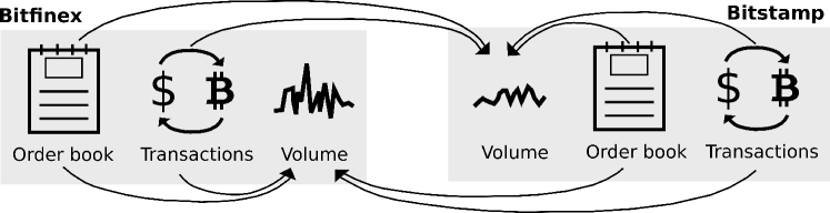
Figure 1: Illustration of the probabilistic volume predicting in the multi-source data setting of Bitfinex and Bitstamp markets. The left and right panel respectively depict the order book and transaction data of each market. The arrows represent the data used to model the volume of each market. Note that the volume information is implicitly contained in the transaction data of one market and thus there is no arrow linking the volumes from the two markets.

The automation of the (cryptocurrency) exchanges lead to the increase of the use of automated trading algo1 ; algo2 via different trading algorithms. An important input for these algos is the prediction of future trading volume. This is important for several reasons. First, trading volume is a proxy for liquidity which in turn is important to quantify transaction costs. Trading algorithms aim at minimizing these costs by splitting orders in order to find a better execution price frei2015optimal ; barzykin2019optimal and the crucial part is the decision of when to execute the orders in such a way to minimize market impact or to achieve certain trading benchmarks (e.g. VWAP) brownlees2010intra ; satish2014predicting ; chen2016forecasting ; bialkowski2008improving ; calvori2013go ; kawakatsu2018direct . Second, when different market venues are available, the algorithm must decide where to post the order and the choice is likely the market where more volume is predicted to be available. Third, volume is also used to model the time-varying price volatility process, whose relation is also known as “Mixture of Distribution Hypothesis” andersen1996-MDH .

In this paper, we study the problem of intraday short-term volume prediction on multi-market of cryptocurrency, as is shown in Fig. 1, intending to obtain not only point estimate but also the uncertainty on the point prediction Chu2015 ; urquhart2016inefficiency ; Katsiampa2017 ; balcilar2017can . Moreover, conventional volume predictions focuses on using data or features from the same market. Since cryptocurrency markets are traded on several markets simultaneously, it is reasonable to use cross-market data not only to enhance the predictive power, but also to help understanding the interaction between markets. In particular, we investigate the exchange rate of Bitcoin (BTC) with a fiat currency (USD) on two liquid markets: Bitfinex and Bitstamp. The first market is more liquid than the second, since its traded volume in the investigated period from June 2018 to November 2018 is $2.5$ times larger. Thus one expects an asymmetric role of the past volume (or other market variables) of one market on the prediction of volume in the other market.

Specifically, the contribution of this paper can be summarized as follows:

• We formulate the cross-market volume prediction as a supervised multi-source learning problem. We use multi-source data, i.e. transactions and limit order books from different markets, to predict the volume of the target market.

• We propose the Temporal Mixture Ensemble (TME), which models individual source’s relation to the target and adaptively adjusts the contribution of the individual source to the target prediction.

• By equipping with modern ensemble techniques, the proposed model can further quantify the predictive uncertainty consisting of the epistemic and aleatoric components, on the predicted volume.

• As main benchmarks for volume dynamics, we use different time-series and machine learning models (clearly with the same regressors/features used in our model). We observe that our dynamic mixture ensemble is often having superior out-of-sample performance on conventional prediction error metrics e.g. root mean square error (RMSE) and mean absolute error (MAE). More importantly, it presents much better calibrated results, evaluated by metrics taking into account predictive uncertainty, i.e. normalized negative log-likelihood (NNLL), uncertainty interval width (IW).

• We discuss the prediction performance conditional to volume. Since our choice of modeling log-volume is tantamount to considering a multiplicative noise model for volumes, when using relative RMSE and MAE machine learning methods outperforms econometric models in providing more accurate forecasts.

The paper is organized as follows: in Sec. 2 we present the investigated markets, the data, and the variables used in the modeling. In Sec. 3 we present our benchmark models. In Sec. 4 we present our empirical investigations on the cryptocurrency markets for the prediction of intraday market volume. Finally, Sec. 5 presents some conclusions and outlook for future work. Most of the technical description of models and algorithms, as well as some additional empirical results, are presented in an appendix.

2 Multiple market cryptocurrency data

Our empirical analyses are performed on a sample of data over the period from May 31, 2018 9:55pm (UTC) until Spetember 30 2018 9:59pm (UTC) from two exchange markets, Bitfinex and Bitstamp, where Bitcoins can be exchanged with US dollars. These markets work through a limit order book, as many conventional exchanges. For each of the two markets we consider two types of data: transaction data and limit order book data.

From transaction data we extract the following features on each 1-min interval:

• Buy volume - number of BTCs traded in buyer initiated transactions

• Sell volume - number of BTCs traded in seller initiated transactions

• Volume imbalance - absolute difference between buy and sell volume

• Buy transactions - number of executed transactions on buy side

• Sell transactions - number of executed transactions on sell side

• Transaction imbalance - absolute difference between buy and sell number of transactions

We remind that a buyer (seller) initiated transaction in a limit order book market is a trade where the initiator is a buy (sell) market order or a buy (sell) limit order crossing the spread.

From limit order book data we extract the following features each minute OB_rev_Porter2013 ; Lillo2016 :

• Spread is the difference between the highest price that a buyer is willing to pay for a BTC (bid) and the lowest price that a seller is willing to accept (ask).

• Ask volume is the number of BTCs on the ask side of order book.

• Bid volume is the number of BTCs on the bid side of order book.

• Imbalance is the absolute difference between ask and bid volume.

• Ask/bid Slope is estimated as the volume until $\delta$ price offset from the best ask/bid price. $\delta$ is estimated by the bid price at the order that has at least 1$\%$, 5$\%$ and 10 $\%$ of orders with the highest bid price.

• Slope imbalance is the absolute difference between ask and bid slope at different values of price associated to $\delta$. $\delta$ is estimated by the bid price at the order that has at least 1$\%$, 5$\%$ and 10 $\%$ of orders with the highest bid price.

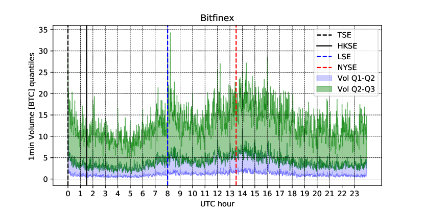
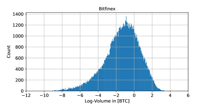
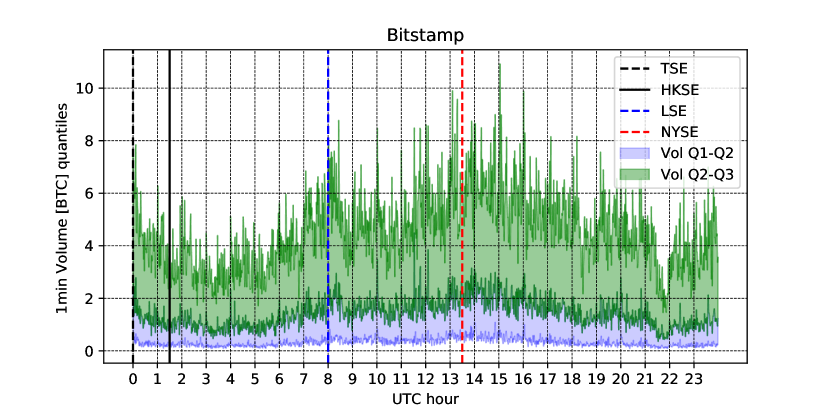
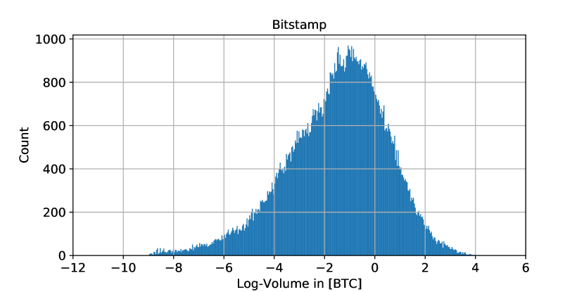
Figure 2: 1st and 3rd panel: interquartile range $Q_{1}-Q_{2}$ and $Q_{2}-Q3$ of intraday 1-min transaction volume of BTC/USD rate on Bitfinex (1st panel) and Bitstamp (3rd panel) market, along with openings of major exchanges (TSE, HKSE, LSE, NYSE) that are denoted with vertical lines. 2nd and 4th panel: histogram of deseasonalized log volume at 1-min resolution. The statistics of these variable are: Bitfinex: mean = -1.3627, variance = 3.7658, skewness = -0.6336, and kurtosis = 0.6886; Bitstamp: mean = -2.4224, variance = 3.9894, skewness = -0.5307, kurtosis = 0.4114.

The target variable that we aim at forecasting is the trading volume of a given target market including both buy and sell volume. In the proposed modeling approaches (described in Sec. 3) we consider different data sources at each time can affect the probability distribution of trading volume in the next time interval in a given market. As is illustrated in Fig. 1, given the setting presented above, there are four sources, namely one for transaction data and one for limit order book data for the two markets.

Before going into the details of models, in order to choose the appropriated variable to investigate, we visualize some characteristics of the data in Fig. 2. In the 1st and 3rd panel, we show the quantiles of intraday 1-min trading volume of BTC/USD rates, for the two different markets. We also show as vertical lines the opening times of four major stock exchanges. Although we do not observe abrupt changes in volume distribution (possibly because cryptocurrency exchanges are weakly related with stock exchanges), some small but significant intraday pattern andersen1997intraday is observed.

For this reason, we pre-process the raw volume data to remove intraday patterns as follows. Let us denote $v_{t}$ the volume traded at the time $t$, in units of Bitcoins. ${I(t)}$ is a mapping function of the time $t$, which returns the intraday time interval index of $t$. We use $a_{I(t)}$ to represent the average of volumes at the same intraday index $I(t)$ across days. Next, to remove intraday patterns, we process the raw volume by taking as modeled variable $y_{t}\triangleq\frac{v_{t}}{a_{I(t)}}$. In practise, in order to avoid leaking information to the training phase, $a_{I(t)}$ is calculated only based on the training data, and shared to both validating and testing data.

The histogram of $\log y_{t}$ for the two markets is shown in the 2nd and 4th panel of Fig. 2 along with first four cumulants of empirical distribution of log-volumes. We observe that the distribution is approximately normal, even if a small negative skew is present. For this reason, as done in the literature (see for example bauwens2008moments , our modeling choice is to consider $y_{t}$ as log-normally distributed.

3 Models

Econometric modeling of intra-daily trading volume relies on a set of empirical regularities brownlees2010intra ; satish2014predicting ; chen2016forecasting of volume dynamics. These include fat tails, strong persistence and an intra-daily clustering around the ”U”-shaped periodic component. Brownlees et al. brownlees2010intra proposed Component Multiplicative Error Model (CMEM), which is the extension of Multiplicative Error Model (MEM) engle2002new . The CMEM volume model has a connection to the component-GARCH ComponentGARCH and the periodic P-GARCH PGARCH . Satish et al. satish2014predicting , proposed four-component volume forecast model composed of: (i) rolling historical volume average, (ii) daily ARMA for serial correlation across daily volumes, (iii) deseasonalized intra-day ARMA volume model and (iv) a dynamic weighted combination of previous models. Chen et al. chen2016forecasting , simplify the multiplicative volume model brownlees2010intra into an additive one by modeling the logarithm of intraday volume with the Kalman filter.

3.1 Problem setting

In this paper, we focus on the probabilistic forecasting including both mean and variance of the intraday volume in the multi-source data setting. We propose the use of TME, presented below, and we benchmark its performance against two econometric baseline models (ARMA-GARCH and ARMAX-GARCH) and one Machine Learning baseline model (Gradient Boosting Machine).

As mentioned above, we assume $y_{t}$ follows the log-normal distribution bauwens2008moments and thus all the models used in the experiments will be developed to learn the log-normal distribution of $y_{t}$. However, our proposed TME is flexible to be equipped with different distributions for the target, and the study in this direction will be the future work.

When evaluating the performance of the forecasting procedure with real data experiments, we choose to use evaluation metrics defined on the original volume $v_{t}$, since in real world application the interest is in forecasting volume rather than log-volume. Finally, for understanding the performance of TME and Machine Learning and econometric baselines in different setups, we will evaluate them using three different time intervals of volumes, namely 1min, 5min and 10min.

Regarding the multi-source data setting, on one hand, it includes the features from the target market. This data is believed to be directly correlated with the target variable. On the other hand, there is an alternative market, which could interact with the target market. Together with the target market, the features from this alternative market constitute the multi-source data.

In this paper, we mainly focus on Bitfinex and Bitstamp markets. For each market, we have the features from both transaction and order book data, thereby leading to $S=4$ data sources. In particular, we indicate with $\mathbf{x}_{s,t}\in\mathbb{R}^{d_{s}}$ the features from source $s$ at time step $t$, and ${d_{s}}$ the dimensionality of source data $s$. Given the list of features presented in Sec. 2, we have $d_{s}=6$ when the source is transaction data in any market, while $d_{s}=13$ for order book data. Then, these multi-source data will be used to model the volume of each market, as is shown in Fig. 1.

3.2 Overview of TME

In this paper, we construct a Temporal Mixture Ensemble (TME), belonging to the class of of mixture models waterhouse1996bayesian ; yuksel2012twenty ; wei2007dynamic ; bazzani2016recurrent ; guo2019exploring , which takes previous transactions and limit order book data OB_rev_Porter2013 ; Lillo2016 from multiple markets simultaneously into account. Though mixture models have been widely used in machine learning and deep learning guo2018bitcoin ; schwab2019granger ; kurle2019multi , they have been hardly explored for prediction tasks in cryptocurrency markets. Moreover, our proposed ensemble of temporal mixtures can provide predictive uncertainty of the target volume by the use of the Stochastic Gradient Descent (SGD) based ensemble technique lakshminarayanan2017simple ; maddox2019simple ; snoek2019can . Predictive uncertainty reflects the confidence of the model over the prediction. It is valuable extra information for model interpretability and reliability. The model developed below is flexible to consume multi-source data of arbitrary number of sources and dimensionalities of individual source data.

In principle, TME exploits latent variables to capture the contributions of different sources of data to the future evolution of the target variable. The source contributing at a certain time depends on the history of all the sources.

For simplicity, we will use one data sample of the target $y_{t}$ to present the proposed model. In reality, the training, validation, and testing data contain the samples collected in a time period. More quantitatively, the generative process of the target variable $y_{t}$ conditional on multi-source data $\{\mathbf{x}_{1,t},\cdots,\mathbf{x}_{S,t}\}$ is formulated as the following probabilistic mixture process:

$$\begin{split}&p(y_{t}|\{\mathbf{x}_{1,<t},\cdots,\mathbf{x}_{S,<t}\},\Theta)\\ =&\sum_{z_{t}=1}^{S}p_{\theta_{s}}(y_{t}|z_{t}=s,\mathbf{x}_{s,<t})\cdot\mathbb{P}_{\omega}(z_{t}=s\,|\mathbf{x}_{1,<t},\cdots,\mathbf{x}_{S,<t}).\end{split}$$ (1)

The latent variable $z_{t}$ is a discrete random variable defined on the set of values $\{1,\cdots,S\}$, each of which represents the corresponding data source. The quantity $p_{\theta_{s}}(y_{t}|z_{t}=s,\mathbf{x}_{s,<t})$ models the predictive probabilistic density of the target based on the historical data $\mathbf{x}_{s,<t}$ from a certain source $s$. The quantity $\mathbb{P}_{\omega}(z_{t}=s\,|\mathbf{x}_{1,<t},\cdots,\mathbf{x}_{S,<t})$ characterize a time-varying categorical distribution dependent on multi-source data. It adaptively adjusts the contribution of the data source specific density $p_{\theta_{s}}(y_{t}|z_{t}=s,\mathbf{x}_{s,<t})$ at each time step. Clearly, it holds $\sum_{s=1}^{S}\mathbb{P}_{\omega}(z_{t}=s\,|\mathbf{x}_{1,<t},\cdots,\mathbf{x}_{S,<t})=1$. Finally, $\Theta\triangleq\{\omega,\theta_{1},\cdots,\theta_{S}\}$ represents the parameters in data source specific components and the latent variable’s probability function, and it will be learned in the training phase discussed below.

3.3 Model specification

We now specify in detail the mathematical formulation of each component in the temporal mixtures. Without loss of generality, we present the following model specification for the volume in cryptocurrency exchange of this paper’s interest.

To specify the model, we need to define the predictive density function of individual sources, i.e. $p_{\theta_{s}}(y_{t}|z_{t}=s,\mathbf{x}_{s,<t})$ and the probability function of latent variable, i.e. $\mathbb{P}_{\omega}(z_{t}=s\,|\mathbf{x}_{1,<t},\cdots,\mathbf{x}_{S,<t})$. We make a general assumption for both these functions that data from different sources are taken within the same time window w.r.t. the target time step. We denote by $h$ the window length, i.e. the number of past time steps which enter in the conditional probabilities. We assume that this value is the same for each source. Eq. 1 is thus simplified as:

$$\begin{split}\sum_{z_{t}=1}^{S}&p_{\theta_{s}}(y_{t}|z_{t}=s,\mathbf{x}_{s,(-h,t)})\cdot\mathbb{P}_{\omega}(z_{t}=s|\mathbf{x}_{1,(-h,t)},\cdots,\mathbf{x}_{S,(-h,t)}),\end{split}$$ (2)

where $\mathbf{x}_{s,(-h,t)}$ represents the data from source $s$ within the time window from $t-h$ to $t-1$ and $\mathbf{x}_{s,(-h,t)}\in\mathbb{R}^{d_{s}\times h}$.

As for $p_{\theta_{s}}(y_{t}|z_{t}=s,\mathbf{x}_{s,(-h,t)})$, due to the non-negative nature of the target volume in cryptocurrency exchange and its statistical properties bauwens2008moments , we choose the log-normal distribution. Given $\mathbf{x}_{s,(-h,t)}\in\mathbb{R}^{d_{s}\times h}$, we choose bi-linear regression to parameterize the mean and variance of the log transformed volume as follows:

$$\ln(y_{t})\,|z_{t}\text{=}s,\mathbf{x}_{s,(-h,t)}\,\sim\,\mathcal{N}\big{(}\mu_{t,s},\sigma_{t,s}^{2})$$ (3)

$$\mu_{t,s}\triangleq L_{\mu,s}^{\top}\cdot\mathbf{x}_{s,(-h,t)}\cdot R_{\mu,s}+b_{\mu,s}$$ (4)

$$\sigma_{t,s}^{2}\triangleq\exp(L_{\sigma,s}^{\top}\cdot\mathbf{x}_{s,(-h,t)}\cdot R_{\sigma,s}+b_{\sigma,s}),$$ (5)

where $L_{\mu,s}$, $L_{\sigma,s}\in\mathbb{R}^{d_{s}}$ and $R_{\mu,s}$, $R_{\sigma,s}\in\mathbb{R}^{h}$. $b_{\mu,s}$, while $b_{\sigma,s}\in\mathbb{R}$ are bias terms. Note that the above parameters are data source specific and then the trainable set of parameters is denoted by $\theta_{s}\triangleq\{L_{\mu,s},L_{\sigma,s},R_{\mu,s},R_{\sigma,s},b_{\mu,s},b_{\sigma,s}\}$.

Based on the properties of log-normal distribution mackay2003information ; cohen1980estimation , the mean and variance of the volume target on the original scale modeled by individual data sources can be derived from the mean and variance of log transformed volume as:

$$\mathbb{E}[{y}_{t}\,|\,z_{t}=s,\mathbf{x}_{s,(-h,t)},\theta_{s}]=\exp\{\mu_{t,s}+\frac{1}{2}\cdot\sigma_{t,s}^{2}\}$$ (6)

and

$$\begin{split}\mathbb{V}[{y}_{t}\,|\,z_{t}=s,\mathbf{x}_{s,(-h,t)},\theta_{s}]=&\exp\{\sigma_{t,s}^{2}-1\}\cdot\exp\{2\cdot\mu_{t,s}+\sigma_{t,s}^{2}\}\end{split}$$ (7)

Then, we define the probability distribution of the latent variable $z_{t}$ using a softmax function as follows:

$$\mathbb{P}_{\omega}(z_{t}=s\,|\,\mathbf{x}_{1,(-h,t)},\cdots,\mathbf{x}_{S,(-h,t)})\triangleq\frac{\exp(\,f_{s}(\mathbf{x}_{s,(-h,t)})\,)}{\exp(\,\sum_{k=1}^{S}f_{k}(\mathbf{x}_{k,(-h,t)})\,)},$$ (8)

where

$$f_{s}(\mathbf{x}_{s,(-h,t)})\triangleq L_{z,s}^{\top}\cdot\mathbf{x}_{s,(-h,t)}\cdot R_{z,s}+b_{z,s}$$ (9)

$\omega\triangleq\{L_{z,s},R_{z,s},b_{z,s}\}_{s=1}^{S}$ denotes the set of trainable parameters regarding the latent variable $z_{t}$, i.e. $L_{z,s},R_{z,s}\in{\mathbb{R}}^{d_{s}}$ and $b_{z,s}\in{\mathbb{R}}$ is a bias term.

In the following, we will present how the distributions modeled by individual data sources and the latent variable will be used to learn the parameters in the training phase and to predict the mean and variance of the target volume in the predicting phase.

3.4 Learning

The learning process of TME is based on SGD optimization ruder2016overview ; kingma2014adam . It is able to give rise to a set of parameter realizations for building the ensemble which has been proven to be an effective technique for enhancing the prediction accuracy as well as enabling uncertainty estimation in previous works lakshminarayanan2017simple ; maddox2019simple .

We first briefly describe the training process of SGD optimization. Denote the set of the parameters by $\Theta\triangleq\{\theta_{1},\cdots,\theta_{S},\omega\}$. The whole training dataset denoted by $\mathcal{D}$ is consisted of data instances, each of which is a pair of $y_{t}$ and $\{\mathbf{x}_{s,(-h,t)}\}_{1}^{S}$. $t$ is a time instant in the period $\{1,\cdots,T\}$.

Starting from a random initialized value of $\Theta$, in each iteration SGD samples a batch of training instances to update the model parameters as follows:

$$\Theta(i)=\Theta(i-1)-\eta\nabla\mathcal{L}(\Theta(i-1);\mathcal{D}_{i}),$$ (10)

where $i$ is the iteration step, $\Theta(i)$ represents the values of $\Theta$ at step $i$, i.e. a snapshot of $\Theta$. $\eta$ is the learning rate, a tunable hyperparameter to control the magnitude of gradient update. $\nabla\mathcal{L}(\Theta(i-1);\mathcal{D}_{i})$ is the gradient of the loss function w.r.t. the model parameters given data batch $\mathcal{D}_{i}$ at iteration $i$. The iteration stops when the loss converges with negligible variation. The model parameter snapshot at the last step or with the best validation performance will be taken as one realization of the model parameters.

The learning process of TME is to minimize the loss function defined by the negative log likelihood of the target volume as:

$$\begin{split}\mathcal{L}(\Theta;\mathcal{D})\triangleq&-\sum^{T}_{t=1}\ln\sum_{z_{t}=1}^{S}p_{\theta_{s}}(y_{t}|z_{t}=s,\mathbf{x}_{s,(-h,t)})\cdot\mathbb{P}_{\omega}(z_{t}=s|\{\mathbf{x}_{s,(-h,t)}\}_{1}^{S})\\ &-\log p(\Theta),\end{split}$$ (11)

where the prior $p(\Theta)$ is viewed as a regularisation term.

By plugging the probability density function of log-normal distribution and Gaussian prior of $\Theta$ as a L2 regularisation, Eq. 11 is further expressed as:

$$\begin{split}&-\sum^{T}_{t=1}\ln\sum_{z_{t}=1}^{S}\frac{1}{y_{t}\sigma_{t,s}\sqrt{2\pi}}\exp\Big{(}-\frac{(\ln y_{t}-\mu_{t,s})^{2}}{2\sigma^{2}_{t,s}}\Big{)}\cdot\mathbb{P}_{\omega}(z_{t}=s|\{\mathbf{x}_{s,(-h,t)}\}_{1}^{S})\\ &-\lambda\left\lVert\Theta\right\rVert^{2}_{2},\end{split}$$ (12)

where $\lambda$ is the hyper-parameter of regularization strength.

In the SGD optimization process, different initialization of $\Theta$ leads to distinct parameter iterate trajectories. Recent studies show that the ensemble of independently initialized and trained model parameters empirically often provide comparable performance on uncertainty quantification w.r.t. sampling and variational inference based methods lakshminarayanan2017simple ; snoek2019can ; maddox2019simple . Our ensemble construction follows this idea by taking a set of model parameter realizations from different training trajectories, and each parameter realization is denoted by $\Theta_{m}=\{\theta_{m,1},\cdots,\theta_{m,S},\omega_{m}\}$. For more algorithmic details about the collecting procedure of these parameter realizations, please refer to the appendix.

3.5 Prediction

In this part, we present the predicting process given model parameter realizations $\{\Theta_{m}\}_{1}^{M}$. We focus on two types of prediction quantities, i.e. mean and variance.

Specifically, the predictive mean of the target in the original scale is defined as:

$$\mathbb{E}[{y}_{t}|\{\mathbf{x}_{s,(-h,t)}\}_{s=1}^{S},\mathcal{D}]\approx\frac{1}{M}\sum_{m=1}^{M}\mathbb{E}[{y}_{t}\,|\,\{\mathbf{x}_{s,(-h,t)}\}_{s=1}^{S},\Theta_{m}],$$ (13)

where $\mathbb{E}[{y}_{t}|\{\mathbf{x}_{s,(-h,t)}\}_{s=1}^{S}\,,\Theta_{m}]$ is the conditional mean given one realization $\Theta_{m}$. In TME, it is a weighted sum of the predictions by individual data sources as:

$$\begin{split}\mathbb{E}[{y}_{t}|\{\mathbf{x}_{s,(-h,t)}\}_{s=1}^{S},\Theta_{m}]=\sum_{s=1}^{S}&\mathbb{P}_{\omega_{m}}(z_{t}=s|\{\mathbf{x}_{s,(-h,t)}\}_{s=1}^{S})\\ &\cdot\mathbb{E}[{y}_{t}|z_{t}=s,\mathbf{x}_{s,(-h,t)},\theta_{m,s}]\end{split}$$ (14)

Apart from the predictive mean, the predictive variance is of great interest as well, since it helps to quantify the uncertainty on the prediction, thereby facilitating the downstream decision making based on the volume predictions.

Given the predictive mean, each data source’s mean and variance defined in Eq. 6, 7 and 13, the predictive variance of the target volume is derived as:

$$\begin{split}&\mathbb{V}({y}_{t}|\{\mathbf{x}_{s,(-h,t)}\}_{s=1}^{S},\mathcal{D})\approx\int_{y}y^{2}p({y}|\{\mathbf{x}_{s,(-h,t)}\}_{s},\mathcal{D})dy-\mathbb{E}^{2}[{y}_{t}|\{\mathbf{x}_{s,(-h,t)}\}_{s=1}^{S},\mathcal{D}]\\ &=\underbrace{\frac{1}{M}\sum_{m=1}^{M}\sum_{s=1}^{S}\mathbb{P}_{\omega_{m}}(z_{t}=s|\cdot)\mathbb{V}(y_{t}|z_{t}=s,\mathbf{x}_{s,(-h,t)},\theta_{m,s})}_{\text{Aleatoric Uncertainty}}+\\ &\underbrace{\frac{1}{M}\sum_{m=1}^{M}\sum_{s=1}^{S}\mathbb{P}_{\omega_{m}}(z_{t}=s|\cdot)\mathbb{E}^{2}[y_{t}|z_{t}=s,\mathbf{x}_{s,(-h,t)},\theta_{m,s})-\mathbb{E}^{2}[y_{t}|\{\mathbf{x}_{s,(-h,t)}\}_{s=1}^{S},\mathcal{D}],}_{\text{Epistemic Uncertainty}}\end{split}$$ (15)

where for clarity of the formula $\mathbb{P}_{\omega_{m}}(z_{t}=s|\{\mathbf{x}_{s,(-h,t)}\}_{s=1}^{S})$ is simplified to $\mathbb{P}_{\omega_{m}}(z_{t}=s|\cdot)$.

Eq. 15 shows that the predictive variance is composed of two types of uncertainties, aleatoric and epistemic uncertainty. The aleatoric part in Eq. 15 stems from variance induced from multi-source data. It captures the noise inherent to the target which could depend on $\mathbf{x}_{s,(-h,t)}$. As a comparison, the classical aleatoric uncertainty (or volatility) estimation model is typically used to estimate the uncertainty solely with the target time series or external features as a whole. It has no mechanism to capture the evolving relevance of multi-source data to the aleatoric uncertainty of the target. The epistemic uncertainty part in Eq. 15 accounts for uncertainty in the model parameters i.e. uncertainty which captures our ignorance about which model generated our collected data. It is also referred to as the model uncertainty.

4 Experiments

In this section, we report the overall experimental evaluation. More detailed results are in the appendix section.

4.1 Data and metrics

Data: We collected the limit order book and transaction data respectively from two exchanges, Bitfinex and Bitstamp and extracted features defined in Sec. 2 from the order book and transactions of each exchange for the period from May 31, 2018 9:55pm (UTC) until September 30, 2018 9:59pm (UTC). Then, for each exchange, we build three datasets of different prediction horizons, i.e. 1min, 5min, 10min, for training and evaluating models. Depending on the prediction horizon, each instance in the dataset contains a target volume and the time-lagged features from order book and transactions of two exchanges. In particular, for Bitfinex, the sizes of datasets for 1min, 5min, 10min are respectively $171727$, $34346$ and $17171$. For Bitstamp, the sizes of datasets are respectively $168743$, $33749$ and $16873$. In all the experiments, data instances are time ordered and we use the first $70\%$ of points for training, the next $10\%$ for validation, and the last $20\%$ of points for out-of-sample testing. Note that all the metrics are evaluated on the out of sample testing data.

For modeling the log-normal distribution, the baseline models and TME need to perform the log-transformation on $y_{t}$ and thus in the data pre-processing step, we have filtered out the data instances with zero trading volume. Empirically, we found out that these zero-volume data instances account for less than $2.25\%$ and $3.98\%$ of the entire dataset for Bitfinex and Bitstamp markets respectively.

For the baseline methods not differentiating the data source of features, each target volume has a feature vector built by concatenating all features from order book and transactions of two markets into one vector. For our TME, each target volume has four groups of features respectively corresponding to the order book and transaction data of two markets.

Metrics: Note that baseline models and TME are trained to learn the log-normal distribution of the deseasonalized volume, however, the following metrics are evaluated on the original scale of the volume, because our aim is to quantify the performance on the real volume scale, that is of more interest for practical purposes.

In the following definitions, $\hat{v}_{t}$ corresponds to the predictive mean of the raw volume. $\overline{T}$ is the number of data instances in the testing dataset. $\hat{v}_{t}$ is derived from the predictive mean of $y_{t}$ multiplied by $a_{I(t)}$, according to the definition of $y_{t}$ in Sec. 3. For baseline models, the predictive mean of $y_{t}$ is derived from the mean of logarithmic transformed $y_{t}$ via Eq. 6 used by individual sources in TME. The predictive mean of $y_{t}$ by TME is shown in Eq.13. The considered performance metrics are:

RMSE: is the root mean square error as $\text{RMSE}=\sqrt{\frac{1}{\overline{T}}\sum_{t=1}^{\overline{T}}(v_{t}-\hat{v}_{t})^{2}}$.

MAE: is mean absolute error as $\text{MAE}=\frac{1}{\overline{T}}\sum_{t=1}^{\overline{T}}|v_{t}-\hat{v}_{t}|$.

NNLL: is the predictive Negative Log-Likelihood of testing instances normalized by the total number of testing points. For the target variable volume, the likelihood of the real $v_{t}$ is that of the corresponding intraday-pattern free $y_{t}$ scaled by $\frac{1}{a_{I(t)}}$, according to the definition in Sec.3. For TME, the likelihood of $y_{t}$ is calculated, as shown in Eq. 12, based on the mixture of log-normal distributions taking into account both predictive mean and variance. For baseline models, the likelihood of $y_{t}$ can be straightforwardly derived from the predictive mean and variance of $\ln y_{t}$  mackay2003information ; cohen1980estimation .

IW: interval width is meant to evaluate the uncertainty around the point prediction, i.e. predictive mean, in probabilistic forecasting. The ideal model is expected to provide tight intervals, which imply the model is confident in the prediction. In this paper, our baseline models and TME involve unimodal and multimodal distributions, i.e. log-normal and mixture of log-normal. As a result, we choose to measure the interval width simply using the variance kuleshov2018accurate . Specifically, IW is defined as the averaged standard deviation of the testing instances. Note that similar to the scaling operation for getting $\hat{v}_{t}$, the standard deviation is obtained via firstly scaling the predictive variance of $y_{t}$ by $a_{I(t)}^{2}$.

4.2 Baseline models and TME setup

As mentioned above, we benchmark the performance of TME against two econometric and one Machine Learning models. We present them below.

ARMA-GARCH is the autoregressive moving average model (ARMA) plus generalized autoregressive conditional heteroskedasticity (GARCH) model brownlees2010intra ; satish2014predicting ; chen2016forecasting . It is aimed to respectively capture the conditional mean and conditional variance of the logarithmic volume. Then, the predictive mean and variance of the logarithmic volume are transformed to the original scale of the volume for evaluation.

The number of autoregressive and moving average lags in ARMA are selected in the range from 1 to 10, by minimization of Akaike Information Criterion, while the orders of lag variances and lag residual errors in GARCH are found to affect the performance negligibly and thus are both fixed to one Hansen2005 . The residual diagnostics for ARMA-GARCH models is given in the appendix Figure 5 and Figure 6.

In Table 1 we report the estimated GARCH parameters in the ARMA-GARCH model on the log-volume, together with the standard errors and the p-value. All parameters are statistically different from zero at all time scales, indicating the significant existence of heteroskedasticity.

Table 1: Statistics of GARCH(1,1) parameters ($\omega$, $\alpha$, $\beta$) on log-volume residuals, trained with ARMA($p,q$)-GARCH(1,1) model for different markets and prediction horizons. (*) indicate p-values $<10^{-5}$ for estimated parameters. Parameters $p,q$, were selected by minimizing AIC and are reported in Tables 2-4.

BITFINEX	$\omega$	Std.Err($\omega$)	$\alpha$	Std.Err($\alpha$)	$\beta$	Std.Err($\beta$)
1 min	0.0177*	0.0011	0.0259*	0.0008	0.9677*	0.0000
5 min	0.0119*	0.0015	0.0218*	0.0017	0.9663*	0.0000
10 min	0.0062*	0.0011	0.0152*	0.0018	0.9762*	0.0000
BITSTAMP	$\omega$	Std.Err($\omega$)	$\alpha$	Std.Err($\alpha$)	$\beta$	Std.Err($\beta$)
1 min	0.0112*	0.0007	0.0203*	0.0006	0.9759*	0.0000
5 min	0.0175*	0.0023	0.0277*	0.0022	0.9561*	0.0000
10 min	0.0262*	0.0056	0.0291*	0.0042	0.9387*	0.0000

ARMAX-GARCH is the variant of ARMA-GARCH by adding external feature terms. In our scenario, external features are obtained by concatenating all features from order book and transaction data of two exchanges into one feature vector. The hyper-parameters in ARMAX-GARCH are selected in the same way as for ARMA-GARCH.

GBM is the gradient boosting machine friedman2001greedy . It has been empirically proven to be highly effective in predictive tasks across different machine learning challenges gulin2011winning ; taieb2014gradient and more recently in financezhou2015evolution ; sun2018novel . The feature vector fed into GBM is also the concatenation of features from order book and transaction data of two markets. The hyper-parameters scikit-learn of GBM are selected by random search in the ranges: number of trees in $[100,\cdots,1000]$, max number of features used by individual trees in $[1.0,\cdots,0.1]$, minimum number of samples of the leaf nodes in $[2,\cdots,9]$, maximum depth of individual trees in $[4,\cdots,9]$, and the learning rate in $[0.05,\cdots,0.005]$.

TME is implemented by TensorFlow . The hyper-parameters tuned by random search are mainly the learning rate in the range $[0.0001,\cdots,0.001]$, batch size in $[10,\cdots,300]$, and the l2 regularization term in $[0.1,\cdots,5.0]$. The number of model parameter realizations for building the ensemble is set to 20. Beyond this number, we found no significant performance improvement.

4.3 Results

In this section, we present the results on the predictions of volume in both markets at different time scales. Tables 2, 3, and  4 show the error metrics on the testing data for the two markets and the four models. We observe that in all cases the smallest RMSE is achieved by TME while the smallest MAE is achieved by GBM. Concerning NNLL, in Bitfinex TME outperforms the other models for 1-min and 5-min cases, while for Bitstamp markets econometirc model have (slightly) lower values. Finally, the smallest IW is always achieved by TME.

The fact that GBM has superior performance on MAE is somewhat expected since GBM has been trained to minimize point prediction, while ARMA-GARCH, ARMAX-GARCH and TME were trained with a maximum likelihood objective.

By comparing RMSE and MAE in both markets, we observe that for ARMA-GARCH model in Bitfinex, external features and extra information from Bitstamp are lowering MAE and RMSE errors (except on 1min interval on Bitfinex market). In Bitstamp market, for ARMAX-GARCH model external features only help on 1-min interval prediction. This phenomenon could indicate the one-directional information relevance across two markets. However, due to the data source specific components and temporal adaptive weighting schema, our TME is able to yield more accurate prediction consistently, compared to ARMA-GARCH.

As for NNLL, similar pattern is observed in ARMA-GARCH family, i.e. additional features impair the NNLL performance instead, while TME retains comparable performance. More importantly, TME has much lower IW. Together with the lower RMSE, it implies that when TME predicts the mean closer to the observation, the predictive uncertainty is also lower. Remind that GBM does not provide probabilistic predictions. Overall we find that TME outperforms quite often the baseline benchmarks, by providing smaller RMSE and tighter intervals.

Table 2: Results of 1-min volume prediction. The arrow symbols indicate the direction of the metrics for better models. GBM model is not providing uncertainty and NNLL and IW results are not available (NA). Results in bold, indicate the minimum errors among models.

BITFINEX MARKET	RMSE $\downarrow$	MAE $\downarrow$	NNLL $\downarrow$	IW $\downarrow$
ARMA(5,5)-GARCH(1,1)	24.547	14.227	2.660	117.348
ARMAX(5,5)-GARCH(1,1)	24.629	14.189	2.664	117.084
GBM	21.026	7.978	NA	NA
TME	20.142	10.204	2.654	44.344
BITSTAMP MARKET	RMSE $\downarrow$	MAE $\downarrow$	NNLL $\downarrow$	IW $\downarrow$
ARMA(3,3)-GARCH(1,1)	14.587	7.688	1.719	97.618
ARMAX(3,3)-GARCH(1,1)	14.292	7.487	1.719	93.943
GBM	11.740	3.515	NA	NA
TME	11.378	4.299	1.720	10.295

Table 3: Results of 5-min volume prediction. The arrow symbols indicate the direction of the metrics for better models. GBM model is not providing uncertainty and NNLL and IW results are not available (NA). Results in bold, indicate the minimum errors among models.

BITFINEX MARKET	RMSE $\downarrow$	MAE $\downarrow$	NNLL $\downarrow$	IW $\downarrow$
ARMA(3,3)-GARCH(1,1)	64.999	39.909	4.642	82.158
ARMAX(3,3)-GARCH(1,1)	64.456	39.150	4.641	79.852
GBM	64.964	32.888	NA	NA
TME	63.855	39.527	4.636	68.748
BITSTAMP MARKET	RMSE $\downarrow$	MAE $\downarrow$	NNLL $\downarrow$	IW $\downarrow$
ARMA(5,4)-GARCH(1,1)	38.300	17.606	3.732	34.797
ARMAX(5,4)-GARCH(1,1)	40.273	18.887	3.766	38.250
GBM	39.196	14.714	NA	NA
TME	38.223	17.287	3.765	29.148

Table 4: Results of 10-min volume prediction. The arrow symbols in the first line indicate the direction of the metrics for better models. GBM model is not providing uncertainty and NNLL and IW results are not available (NA)

BITFINEX MARKET	RMSE $\downarrow$	MAE $\downarrow$	NNLL $\downarrow$	IW $\downarrow$
ARMA(3,2)-GARCH(1,1)	112.872	72.505	5.409	124.890
ARMAX(3,2)-GARCH(1,1)	111.987	71.149	5.373	121.346
GBM	110.197	61.506	NA	NA
TME	109.878	68.382	5.386	114.195
BITSTAMP MARKET	RMSE $\downarrow$	MAE $\downarrow$	NNLL $\downarrow$	IW $\downarrow$
ARMA(3,2)-GARCH(1,1)	66.486	31.942	4.452	51.228
ARMAX(3,2)-GARCH(1,1)	68.067	32.795	4.457	52.780
GBM	67.128	27.719	NA	NA
TME	66.234	31.460	4.507	49.972

In order to disentangle the different contributions to TME predictions and, at the same time, understanding why choosing different predicting features at each time step is important, we present in Fig. 3 and Fig. 4 the predictive volume and uncertainty of 5-min volume prediction in a sample time period of the testing data for the two markets.

Panel (a) shows how well the TME (pointwise and interval) predictions follows the actual data. The TME is able to quantify at each time step the contribution of each source to the target forecasting. In Panel(b) we show the dynamical contribution scores of the four sources. These scores are simply the average of the probability of the latent variable value corresponding to each data source, i.e. $z_{t}=s$. We notice that the relative contributions varies with time and we observe that the external order book source from the less liquid market (Bitstamp) does not contribute much to predictions. On the contrary, in Panel (b) of Fig. 4, where the data for Bitstamp are shown, external order book and external transaction features from the more liquid market (Bitfinex) play a more dominant role. Then, when we further look at the predictions by individual data sources in TME, see Panel(c)-(f), what we observe is in line with the pattern of contribution scores in Panel(b). For instance, the component model in TME responsible for the data source from more liquid Bitfinex captures more uncertainty, thereby being given high contribution scores in the volatile period. The addition of the features from the other markets allows to shrink the uncertainty intervals. We have also repeated these experiments for 1-min and 10-min volume prediction. The results are collected in the figures and tables in the appendix section.

Figure 3: Visualization of TME in a sample period of Bitfinex for 5-min volume predicting. Panel(a): Predictive mean $\pm$ two times standard deviation (left-truncated at zero) and the volume observations. Panel(b): Data source contribution scores (i.e. average of latent variable probabilities) over time. Panel(c)-(f): Each data source’s predictive mean $\pm$ two times standard deviation (left-truncated at zero). The color of each source’s plot corresponds to that of the contribution score in Panel(b). (best viewed in colors)

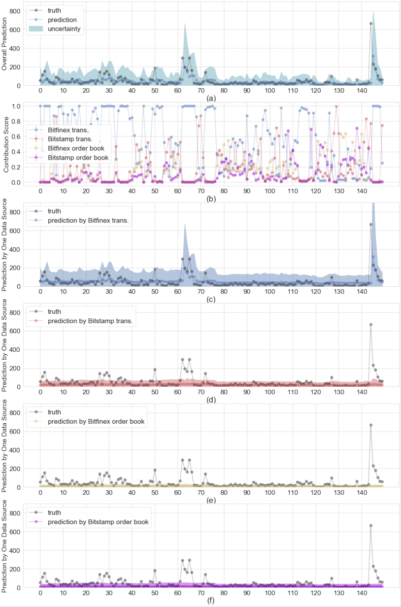
Figure 4: Visualization of TME in a sample period of Bitstamp for 5-min volume predicting. Panel(a): Predictive mean $\pm$ two times standard deviation (left-truncated at zero) and the volume observations. Panel(b): Data source contribution scores (i.e. average of latent variable probabilities) over time. Panel(c)-(f): Each data source’s predictive mean $\pm$ two times standard deviation (left-truncated at zero). The color of each source’s plot corresponds to that of the contribution score in Panel(b). (best viewed in colors)

Finally, we discuss how well the different predictors perform conditionally to the volume size. To this end, we compute for each model, market, and time interval the RMSE and MAE conditional to the volume quartile. However, finding the suitable metrics to compare forecasting performance of a model across different quartiles is a subtle issue. Take for example a linear model for the log-volume. When considering it as a model for (linear) volume, it is clear that the additive noise in the log-volume becomes multiplicative in linear volume. Thus the RMSE conditional to volume becomes proportional to (or increasing as a power-law of) the volume and therefore one expects to see RMSE for high quartiles to be larger than the one for bottom quartiles. This is exactly what we observe in Table 5 for 5 min horizons (for 1 and 10 min, see the appendix) when looking at RMSE and MAE.

In order to take into account this statistical effect, essentially caused by the choice of modeling log-volume and presenting eroor metrics for linear volume, in Table 5 we show also relative error metrics, namely relative root mean squared error (RelRMSE) and mean absolute percentage error (MAPE) conditioned to volume quartile. (RelRMSE is defined as $\sqrt{\frac{1}{\overline{T}}\sum_{t=1}^{\overline{T}}(\frac{v_{t}-\hat{v}_{t}}{v_{t}})^{2}}$), and MAPE is defined as $\frac{1}{\overline{T}}\sum_{t=1}^{\overline{T}}|\frac{v_{t}-\hat{v}_{t}}{v_{t}}|$.) In this case the scenario changes completely. First, across all models the relative error is smaller for top volume quartiles and larger for bottom quartiles. Especially relative errors for the lowest quartile are large, likely because small volumes at the denominator create large fluctuations. Second, and more important, TME outperforms mostly in Q4, while GBM is superior in Q1, Q2, and Q£ frequently. The difference between models in Q4 is somewhat smaller, while in Q1-Q3 the out-performance of machine learning methods is up to a factor $2$ with respect to econometric methods. Thus also when considering large volumes and considering relative errors, TME and GBM provide more accurate predictions.

Table 5: 5-min volume prediction errors conditional on the quartile of the true volume values. Measures: RMSE Qx – root mean squared error conditioned on x-th quantile, RelRMSE Qx – relative root mean squared error conditioned on x-th quantile, MAE Qx – mean average error conditioned on x-th quantile, MAPE Qx – mean absolute percentage error conditioned on x-th quantile.

BITFINEX MARKET	RMSE Q1	RMSE Q2	RMSE Q3	RMSE Q4
ARMA-GARCH	32.862	38.594	43.073	111.660
ARMAX-GARCH	31.939	36.887	41.005	112.020
GBM	17.632	17.332	22.056	125.604
TME	32.200	32.976	35.928	112.280
	RelRMSE Q1	RelRMSE Q2	RelRMSE Q3	RelRMSE Q4
ARMA-GARCH	19.417	2.769	1.299	0.609
ARMAX-GARCH	18.845	2.657	1.243	0.594
GBM	12.672	1.268	0.615	0.623
TME	26.235	2.378	1.098	0.578
	MAE Q1	MAE Q2	MAE Q3	MAE Q4
ARMA-GARCH	26.781	28.635	29.622	74.576
ARMAX-GARCH	26.145	27.625	28.190	74.612
GBM	14.719	11.985	16.674	88.122
TME	26.317	28.784	23.338	74.484
	MAPE Q1	MAPE Q2	MAPE Q3	MAPE Q4
ARMA-GARCH	9.506	2.003	0.871	0.497
ARMAX-GARCH	9.272	1.935	0.831	0.493
GBM	5.717	0.846	0.460	0.570
TME	11.424	1.823	0.690	0.503
BITSTAMP MARKET	RMSE Q1	RMSE Q2	RMSE Q3	RMSE Q4
ARMA-GARCH	13.465	15.304	16.199	72.046
ARMAX-GARCH	14.2	16.835	20.0009	74.8532
GBM	6.432	6.679	8.732	77.317
TME	13.617	14.492	14.583	73.778
	RelRMSE Q1	RelRMSE Q2	RelRMSE Q3	RelRMSE Q4
ARMA-GARCH	22.171	2.563	1.175	0.671
ARMAX-GARCH	24.259	2.784	1.429	0.889
GBM	12.578	1.154	0.596	0.658
TME	29.289	2.429	1.084	0.586
	MAE Q1	MAE Q2	MAE Q3	MAE Q4
ARMA-GARCH	10.668	11.648	11.020	37.094
ARMAX-GARCH	11.0917	12.275	12.1831	39.9903
GBM	5.037	4.575	6.705	42.506
TME	11.778	11.342	10.138	36.827
	MAPE Q1	MAPE Q2	MAPE Q3	MAPE Q4
ARMA-GARCH	11.049	1.910	0.792	0.523
ARMA-GARCH	11.656	2.007	0.873	0.603
GBM	5.838	0.755	0.456	0.599
TME	14.117	1.871	0.720	0.493

5 Conclusion and discussion

In this paper, we analyzed the problem of predicting trading volume and its uncertainty in cryptocurrency exchange markets. The main innovations proposed in this paper are (i) the use of transaction and order book data from different markets and (ii) the use of TME, a class of models able to identify at each time step the set of data locally more useful in predictions.

By investigating data from BTC/USD exchange markets, we found that time series models of the ARMA-GARCH family do provide fair basic predictions for volume and its uncertainty, but when external data (e.g. from order book and/or from other markets) are added, the prediction performance does not improve significantly. Our analysis suggests that this might be due to the fact that the contribution of this data to the prediction could be not constant over time, but depending on the ”market state”. The temporal mixture ensemble model is designed precisely to account for such a variability. Indeed we find that this method outperforms time series models both in point and in interval predictions of trading volume. Moreover, especially when compared to other machine learning methods, the temporal mixture approach is significantly more interpretable, allowing the inference of the dynamical contributions from different data sources as a core part of the learning procedure. This has important potential implications for decision making in economics and finance.

Also when conditioning to volume quartile, TME and GBM outperform econometric methods especially in the first three quartiles. For large volumes, likely due to the presence of unexpected bursts of volume which are very challenging to forecast, the performances of the methods are more comparable. However by using relative RMSE and MAPE the forecasting errors for large volumes are small.

Finally, although the method has been proposed and tested for cryptocurrency volume in two specific exchanges, we argue that it can be successfully applied (in future work) to other cryptocurrencies and to more traditional financial assets.

6 Appendix

6.1 ARMAX-GARCH

As mentioned, our benchmarks belong to the ARMAX-GARCH class with external regressors. More specifically, the volume process is modelled with the following:

$$\Phi(L)(\ln(y_{t})-\mu_{t})=\Theta(L)\epsilon_{t},$$ (16)

where $\Phi(L)$, $\Theta(L)$ denote polynomials of the lag operator $L$. The time varying mean $\mu_{t}$ is modeled as

$$\mu_{t}=\mu+\sum_{s=1}^{S}\sum_{j=1}^{d_{s}}\psi_{s,j}x_{s,t-1}(j)$$ (17)

where $x_{s,t-1}(j)$ denotes the $j$-th feature from external feature vector $\mathbf{x}_{s,t-1}$ at time $t-1$ from source $s$. The total number of sources $S=4$, which includes transactions and limit order book data of the two markets. Since variance of volume might exhibit time clustering, we assume that the residuals $\epsilon_{t}$ are modelled by a GARCH process GARCH ; brownlees2010intra ; satish2014predicting ; chen2016forecasting :

$$\epsilon_{t}=\sigma_{t}e_{t}~{}~{}~{}~{}~{}~{}~{}e_{t}\sim\mathcal{N}(0,1)$$ (18)

$$\sigma_{t}^{2}=\omega+\alpha\epsilon_{t-1}^{2}+\beta\sigma_{t-1}^{2}$$ (19)

6.2 Gradient boosting

In the following, we summarize how GBM is the used in the context of volume predicting. For more details of GBM, we suggest referring to friedman2001greedy .

At time $t$, the target label is $u_{t}=\ln{y_{t+1}}$, is the logarithm of deseasonalized volume at next time segment. Gradient boosting approximates the target variable $u_{t}$ with a function $F(\mathbf{x}_{t})$ that has the following additive expansion (similar to other functional approximation methods like radial basis functions, neural networks, wavelets, etc.):

$$\hat{u_{t}}=F(\mathbf{x}_{t})=\sum_{m=0}^{M}\beta_{m}h(\mathbf{x}_{t};\mathbf{a}_{m}),$$ (20)

where $\mathbf{x}_{t}$ denotes the feature vector, that is constructed as a concatenation from different sources $\mathbf{x}_{t}=(\mathbf{x}_{s=1,(-h,t)},\mathbf{x}_{s=2,(-h,t)},\mathbf{x}_{s=3,(-h,t)},\mathbf{x}_{s=4,(-h,t)})$.

For a given training sample $\{u_{t},\mathbf{x}_{t}\}_{t=1}^{T}$, our goal is to find a function $F^{*}(\mathbf{x})$ such that the expected value of loss function $\frac{1}{2}(u-F(\mathbf{x}))^{2}$ (squared loss) is minimized over the joint distribution of $\{u,\mathbf{x}\}$

$$F^{*}(\mathbf{x})=\operatorname*{arg\,min}_{F(x)}\mathbb{E}_{u,\mathbf{x}}(u-F(\mathbf{x}))^{2}.$$ (21)

Under the additive expansion $F(\mathbf{x})=\sum_{m=0}^{M}\beta_{m}h(\mathbf{x};\mathbf{a}_{m})$ with parameterized functions $h(\mathbf{x};\mathbf{a}_{m})$, we proceed by making the initial guess $F_{0}(\mathbf{x})=\operatorname*{arg\,min}_{c}\sum_{t=1}^{T}(u_{t}-c)^{2}$ and then parameters are jointly fit in a forward incremental way $m=1,...,M$:

$$(\beta_{m},\mathbf{a}_{m})=\operatorname*{arg\,min}_{\beta,\mathbf{a}}\sum_{t=1}^{T}(u_{t}-(F_{m-1}(\mathbf{x}_{t})+\beta h(\mathbf{x}_{t};\mathbf{a})))^{2}$$ (22)

and

$$F_{m}(\mathbf{x}_{t})=F_{m-1}(\mathbf{x}_{t})+\beta_{m}h(\mathbf{x}_{t};\mathbf{a}_{m}).$$ (23)

First, the function $h(\mathbf{x}_{t};\mathbf{a})$ is fit by least-squares to the pseudo-residuals $\widetilde{u}_{t,m}$

$$\mathbf{a}_{m}=\operatorname*{arg\,min}_{\mathbf{a},\rho}\sum_{t=1}^{T}[\widetilde{u}_{t,m}-\rho h(\mathbf{x}_{t};\mathbf{a})]^{2},$$ (24)

which at stage $m$ is a residual $\widetilde{u}_{t,m}=(u_{t}-F_{m-1}(\mathbf{x}_{t}))$. Pseudo-residual at arbitrary stage is defined as

$$\widetilde{u}_{t,m}=-\left[\frac{\partial\frac{1}{2}(u_{t}-F(\mathbf{x}_{t}))^{2}}{\partial F(\mathbf{x}_{t})}\right]_{F(\mathbf{x})=F_{m-1}(\mathbf{x})}.$$ (25)

The parameter $\rho$ acts as the optimal learning rate in the steepest-descent step, for more details check friedman2001greedy . Now, we just find the coefficient $\beta_{m}$ for the expansion as

$$\beta_{m}=\operatorname*{arg\,min}_{\beta}\sum_{t=1}^{T}\frac{1}{2}(u_{t}-(F_{m-1}+\beta h(\mathbf{x}_{t};\mathbf{a}_{m})))^{2}.$$ (26)

Each base learner $h(\mathbf{x}_{t};\mathbf{a}_{m})$, parameterized with $\mathbf{a}_{m}$ partitions the feature space $\mathbf{x}_{t}\in\mathbf{X}$ into $L_{m}$-disjoint regions $\{R_{l,m}\}_{1}^{L_{m}}$ and predicts a separate constant value in each:

$$h(\mathbf{x}_{t};\{R_{l,m}\}_{1}^{L_{m}})=\sum_{l=1}^{L_{m}}\bar{u}_{l,m}\mathbf{1}(\mathbf{x}_{t}\in R_{l,m}),$$ (27)

where $\bar{u}_{l,m}$ is the mean value of pseudo-residual (eq. 25) in each region $R_{l,m}$

$$\bar{u}_{l,m}=\frac{\sum_{t=1}^{T}\widetilde{u}_{t,m}\mathbf{1}[\mathbf{x}_{t}\in R_{l,m}]}{\sum_{t=1}^{T}\mathbf{1}[\mathbf{x}_{t}\in R_{l,m}]}.$$ (28)

We have used the GBM implementation from Scikit-learn library scikit-learn for all our experiments. Furthermore, note that different variants of tree boosting have been empirically proven to be state-of-the-art methods in predictive tasks across different machine learning challenges bentejac2020comparative ; chen2016xgboost ; lu2020randomized ; taieb2014gradient ; gulin2011winning and more recently in financezhou2015evolution ; sun2018novel .

6.3 SGD-based model ensemble

In stochastic gradient descent (SGD) based optimization, stochasticity comes from two places:

• SGD trajectory. The iterates $\{\Theta(0),\cdots,\Theta(i)\}$ forms a exploratory trajectory, as $\Theta(i)$ is updated by randomly data sample $\mathcal{D}_{i}$. Recent works mandt2017stochastic ; gur2018gradient studied the connection of trajectory iterates to an approximate Markov chain Monte Carlo sampler by analyzing the dynamics of SGD.

• Model initialization. Different initialization of model parameters, i.e. $\Theta(0)$, leads to distinct trajectories. It has been shown that ensembles of independently initialized and trained models empirically often provide comparable performance in prediction and uncertainty quantification w.r.t. sampling and variational inference based methods, even though it does not apply conventional Bayesian grounding lakshminarayanan2017simple ; snoek2019can .

In this paper, we make a hybrid approach, that uses both sources of stochasticity to obtain parameter realizations $\{\Theta_{m}\}$ as follows:

$$\{\Theta_{m}\}\triangleq\bigcup_{j}\{\Theta^{j}(i),\cdots,\Theta^{j}(I)\}$$ (29)

Eq. 29 indicates that from each independently trained SGD trajectory (indexed by $j$), we skip the beginning few epochs as a ”burn-in” step. We choose the remaining as samples from this trajectory. Then, we further take the union of samples from independent trajectories as the samples used by the inference in Sec. 3.5.

In our experiments, we use Adam optimization, a variant of SGD, which has been widely used in machine learning kingma2014adam . We found that $5$ to $25$ independent training processes can give rise to decently accurate and calibrated forecasting. Moreover, by parallel computing on GPU, we perform each training process in parallel without loss of efficiency.

6.4 Residual diagnostics of ARMA-GARCH models

In Figure 5 and Figure 6, we show auto-correlation function of the residuals for Bitfinex and Bitstamp market, respectively. In all cases of ARMA($p,q$)-GARCH(1,1) models, parameters $p,q$ were fitted to Akaike Information Criterion. For 1min, 5min and 10min target the majority of residuals ACF are within significance area and only a small number falls very close to the significance area, which implies that the residuals are almost uncorrelated and models well specified.

\begin{overpic}[width=411.93767pt]{figures/ACF_residuals_market1_tar10ARMA-GARCH.pdf} \put(3.0,98.0){\large{}} \end{overpic}

\begin{overpic}[width=411.93767pt]{figures/ACF_residuals_market1_tar5_ARMA-GARCH.pdf} \put(3.0,98.0){\large{}} \end{overpic}

\begin{overpic}[width=411.93767pt]{figures/ACF_residuals_market1_tar1_ARMA-GARCH.pdf} \put(3.0,98.0){\large{}} \end{overpic}

Figure 5: Residual diagnostics for Bitfinex market: First row ACF of ARMA(3,2)-GARCH(1,1) model residuals on log-volume 10 min. Second row ACF of ARMA(3,3)-GARCH(1,1) model residuals on log-volume 5 min. Third row ACF of ARMA(5,5)-GARCH(1,1) model residuals on log-volume 1 min.

\begin{overpic}[width=411.93767pt]{figures/ACF_residuals_market2_tar10ARMA-GARCH.pdf} \put(3.0,98.0){\large{}} \end{overpic}

\begin{overpic}[width=411.93767pt]{figures/ACF_residuals_market2_tar5_ARMA-GARCH.pdf} \put(3.0,98.0){\large{}} \end{overpic}

\begin{overpic}[width=411.93767pt]{figures/ACF_residuals_market2_tar1_ARMA-GARCH.pdf} \put(3.0,98.0){\large{}} \end{overpic}

Figure 6: Residual diagnostics for Bitstamp market: First row ACF of ARMA(3,2)-GARCH(1,1) model residuals on log-volume 10 min. Second row ACF of ARMA(5,4)-GARCH(1,1) model residuals on log-volume 5 min. Third row ACF of ARMA(3,3)-GARCH(1,1) model residuals on log-volume 1 min.

6.5 Disentangling TME contributions on 1- and 10-min intervals

We report in Figs. 7 and 8 the contributions to TME prediction in the two markets when the sampling interval is 1 minute, while in Figs. 9 and 10 the same figures for 10 min intervals.

Figure 7: Visualization of TME in a sample period of Bitfinex for 1-min volume predicting. Panel(a): Predictive mean $\pm$ two times standard deviation (left-truncated at zero) and the volume observations. Panel(b): Data source contribution scores (i.e. average of latent variable probabilities) over time. Panel(c)-(f): Each data source’s predictive mean $\pm$ two times standard deviation (left-truncated at zero). The color of each source’s plot corresponds to that of the contribution score in Panel(b). (best viewed in colors)

Figure 8: Visualization of TME in a sample period of Bitstamp for 1-min volume predicting. Panel(a): Predictive mean $\pm$ two times standard deviation (left-truncated at zero) and the volume observations. Panel(b): Data source contribution scores (i.e. average of latent variable probabilities) over time. Panel(c)-(f): Each data source’s predictive mean $\pm$ two times standard deviation (left-truncated at zero). The color of each source’s plot corresponds to that of the contribution score in Panel(b). (best viewed in colors)

Figure 9: Visualization of TME in a sample period of Bitfinex for 10-min volume predicting. Panel(a): Predictive mean $\pm$ two times standard deviation (left-truncated at zero) and the volume observations. Panel(b): Data source contribution scores (i.e. average of latent variable probabilities) over time. Panel(c)-(f): Each data source’s predictive mean $\pm$ two times standard deviation (left-truncated at zero). The color of each source’s plot corresponds to that of the contribution score in Panel(b). (best viewed in colors)

Figure 10: Visualization of TME in a sample period of Bitstamp for 10-min volume predicting. Panel(a): Predictive mean $\pm$ two times standard deviation (left-truncated at zero) and the volume observations. Panel(b): Data source contribution scores (i.e. average of latent variable probabilities) over time. Panel(c)-(f): Each data source’s predictive mean $\pm$ two times standard deviation (left-truncated at zero). The color of each source’s plot corresponds to that of the contribution score in Panel(b). (best viewed in colors)

6.6 Volume predictions conditional to volume quartile

Table 6 and 7 show the performance of the forecast conditioned to volume quartile for the four models and the two markets. As in Table 5 in the main text, we present both absolute metrics (RMSE and MAE) and relative ones (relative MSE and MAPE).

Table 6: 1-min volume prediction errors conditional on the quantile of the true volume values. Measures: RMSE Qx – root mean squared error conditioned on x-th quantile, RelRMSE Qx – relative root mean squared error conditioned on x-th quantile, MAE Qx – mean average error conditioned on x-th quantile, MAPE Qx – mean absolute percentage error conditioned on x-th quantile.

BITFINEX MARKET	RMSE Q1	RMSE Q2	RMSE Q3	RMSE Q4
ARMA-GARCH	13.618	17.314	20.287	38.903
ARMAX-GARCH	13.601	17.350	20.206	39.141
GBM	2.159	2.907	4.323	41.671
TME	8.700	10.032	10.154	36.916
	RelRMSE Q1	RelRMSE Q2	RelRMSE Q3	RelRMSE Q4
ARMA-GARCH	93998.678	16.755	4.992	1.427
ARMAX-GARCH	96451.132	16.508	4.973	1.425
GBM	22735.646	2.764	0.968	0.754
TME	26968.219	9.269	2.539	0.737
	MAE Q1	MAE Q2	MAE Q3	MAE Q4
ARMA-GARCH	9.173	11.300	12.659	23.777
ARMAX-GARCH	9.158	11.249	12.556	23.791
GBM	1.540	1.665	3.054	25.652
TME	8.225	8.620	7.252	20.629
	MAPE Q1	MAPE Q2	MAPE Q3	MAPE Q4
ARMA-GARCH	1319.606	10.151	2.989	0.858
ARMAX-GARCH	1344.985	10.097	2.966	0.855
GBM	296.446	1.502	0.646	0.707
TME	318.682	7.372	1.692	0.568
BITSTAMP MARKET	RMSE Q1	RMSE Q2	RMSE Q3	RMSE Q4
ARMA-GARCH	8.2704	8.9885	11.0034	24.1002
ARMAX-GARCH	7.9412	8.6546	10.5348	23.8335
GBM	0.929	1.085	1.721	23.373
TME	3.047	3.426	3.540	22.005
	RelRMSE Q1	RelRMSE Q2	RelRMSE Q3	RelRMSE Q4
ARMA-GARCH	16842.969	27.709	6.423	1.974
ARMAX-GARCH	16501.630	26.679	6.135	1.923
GBM	2082.545	3.190	0.845	0.786
TME	7279.497	10.951	2.107	0.696
	MAE Q1	MAE Q2	MAE Q3	MAE Q4
ARMA-GARCH	5.400	6.125	7.003	12.223
ARMAX-GARCH	5.239	5.944	6.778	11.985
GBM	0.599	0.605	1.316	11.540
TME	2.664	2.780	2.259	9.615
	MAPE Q1	MAPE Q2	MAPE Q3	MAPE Q4
ARMA-GARCH	1043.922	17.211	3.891	1.097
ARMAX-GARCH	1018.872	16.694	3.767	1.066
GBM	118.256	1.720	0.632	0.741
TME	500.100	8.035	1.301	0.571

Table 7: 10-min volume prediction errors conditional on the quartile of the true volume values. Measures: RMSE Qx – root mean squared error conditioned on x-th quantile, RelRMSE Qx – relative root mean squared error conditioned on x-th quantile, MAE Qx – mean average error conditioned on x-th quantile, MAPE Qx – mean absolute percentage error conditioned on x-th quantile.

BITFINEX MARKET	RMSE Q1	RMSE Q2	RMSE Q3	RMSE Q4
ARMA-GARCH	61.494	70.540	74.188	191.332
ARMAX-GARCH	59.438	67.474	71.237	192.155
GBM	39.380	39.576	46.774	207.957
TME	57.252	64.705	67.354	185.136
	RelRMSE Q1	RelRMSE Q2	RelRMSE Q3	RelRMSE Q4
ARMA-GARCH	9.262	1.998	1.037	0.544
ARMAX-GARCH	8.822	1.911	0.990	0.538
GBM	6.154	1.136	0.587	0.571
TME	11.434	1.878	0.945	0.543
	MAE Q1	MAE Q2	MAE Q3	MAE Q4
ARMA-GARCH	50.542	54.148	53.169	131.891
ARMAX-GARCH	48.985	52.116	51.257	132.081
GBM	33.788	28.760	34.892	148.550
TME	46.680	48.797	43.890	128.578
	MAPE Q1	MAPE Q2	MAPE Q3	MAPE Q4
ARMA-GARCH	5.109	1.503	0.705	0.462
ARMAX-GARCH	4.938	1.448	0.678	0.461
GBM	3.561	0.804	0.434	0.518
TME	6.739	1.499	0.590	0.465
BITSTAMP MARKET	RMSE Q1	RMSE Q2	RMSE Q3	RMSE Q4
ARMA-GARCH	25.000	27.672	27.541	124.527
ARMAX-GARCH	24.963	29.748	29.545	126.985
GBM	14.355	14.700	16.749	131.497
TME	25.469	27.221	24.905	123.804
	RelRMSE Q1	RelRMSE Q2	RelRMSE Q3	RelRMSE Q4
ARMA-GARCH	7.210	1.860	0.949	0.619
ARMAX-GARCH	6.926	1.974	0.984	0.739
GBM	5.638	0.993	0.541	0.625
TME	12.308	1.838	0.858	0.574
	MAE Q1	MAE Q2	MAE Q3	MAE Q4
ARMA-GARCH	20.014	21.343	19.398	66.899
ARMAX-GARCH	19.633	21.685	19.718	70.021
GBM	11.622	10.490	12.965	75.674
TME	21.233	20.034	17.787	64.918
	MAPE Q1	MAPE Q2	MAPE Q3	MAPE Q4
ARMA-GARCH	4.866	1.410	0.646	0.487
ARMAX-GARCH	4.716	1.429	0.653	0.528
GBM	3.341	0.695	0.414	0.555
TME	7.205	1.457	0.550	0.478

References

- (1) A. Urquhart, “The inefficiency of bitcoin,” Economics Letters, vol. 148, pp. 80–82, 2016.
- (2) W. Bolt, “On the value of virtual currencies,” SSRN Electronic Journal, 2016.
- (3) E.-T. Cheah and J. Fry, “Speculative bubbles in bitcoin markets? an empirical investigation into the fundamental value of bitcoin,” Economics Letters, vol. 130, pp. 32–36, 2015.
- (4) J. Chu, S. Nadarajah, and S. Chan, “Statistical analysis of the exchange rate of bitcoin,” PLOS ONE, vol. 10, no. 7, pp. 1–27, 2015.
- (5) J. Donier and J.-P. Bouchaud, “Why do markets crash? bitcoin data offers unprecedented insights,” PLOS ONE, vol. 10, pp. 1–11, 2015.
- (6) P. Ciaian, M. Rajcaniova, and d. Kancs, “The economics of bitcoin price formation,” Applied Economics, vol. 48, pp. 1799–1815, 2016.
- (7) D. Ron and A. Shamir, “Quantitative analysis of the full bitcoin transaction graph,” in International Conference on Financial Cryptography and Data Security. Springer, 2013, pp. 6–24.
- (8) H. Jang and J. Lee, “An empirical study on modeling and prediction of bitcoin prices with bayesian neural networks based on blockchain information,” IEEE Access, vol. 6, pp. 5427–5437, 2018.
- (9) M. Amjad and D. Shah, “Trading bitcoin and online time series prediction,” in NIPS 2016 Time Series Workshop, 2017, pp. 1–15.
- (10) L. Alessandretti, A. ElBahrawy, L. M. Aiello, and A. Baronchelli, “Machine learning the cryptocurrency market,” arXiv preprint arXiv:1805.08550, 2018.
- (11) T. Guo, A. Bifet, and N. Antulov-Fantulin, “Bitcoin volatility forecasting with a glimpse into buy and sell orders,” in 2018 IEEE International Conference on Data Mining (ICDM). IEEE, 2018, pp. 989–994.
- (12) D. Garcia and F. Schweitzer, “Social signals and algorithmic trading of bitcoin,” Royal Society Open Science, vol. 2, no. 9, p. 150288, 2015.
- (13) S. Wheatley, D. Sornette, T. Huber, M. Reppen, and R. N. Gantner, “Are bitcoin bubbles predictable? combining a generalized metcalfe’s law and the log-periodic power law singularity model,” Royal Society open science, vol. 6, no. 6, p. 180538, 2019.
- (14) J.-C. Gerlach, G. Demos, and D. Sornette, “Dissection of bitcoin’s multiscale bubble history from january 2012 to february 2018,” Royal Society open science, vol. 6, no. 7, p. 180643, 2019.
- (15) N. Antulov-Fantulin, D. Tolic, M. Piskorec, Z. Ce, and I. Vodenska, “Inferring short-term volatility indicators from the bitcoin blockchain,” in International Conference on Complex Networks and their Applications. Springer, 2018, pp. 508–520.
- (16) D. Kondor, I. Csabai, J. Szule, M. Posfai, and G. Vattay, “Inferring the interplay between network structure and market effects in bitcoin,” New Journal of Physics, vol. 16, p. 125003, 2014.
- (17) A. ElBahrawy, L. Alessandretti, A. Kandler, R. Pastor-Satorras, and A. Baronchelli, “Evolutionary dynamics of the cryptocurrency market,” Royal Society Open Science, vol. 4, no. 11, p. 170623, 2017.
- (18) S. Nakamoto, “Bitcoin: A peer-to-peer electronic cash system,” 2008. [Online]. Available: http://bitcoin.org/bitcoin.pdf
- (19) J. W. Bos, J. A. Halderman, N. Heninger, J. Moore, M. Naehrig, and E. Wustrow, “Elliptic curve cryptography in practice,” in International Conference on Financial Cryptography and Data Security. Springer, 2014, pp. 157–175.
- (20) H. Mayer, “Ecdsa security in bitcoin and ethereum: a research survey,” CoinFaabrik, June, vol. 28, p. 126, 2016.
- (21) M. Jakobsson and A. Juels, “Proofs of work and bread pudding protocols,” in Secure information networks. Springer, 1999, pp. 258–272.
- (22) E. Baumöhl, “Are cryptocurrencies connected to forex? a quantile cross-spectral approach,” Finance Research Letters, vol. 29, pp. 363 – 372, 2019.
- (23) A. P. Chaboud, B. Chiquoine, H. E., and C. Vega, “Rise of the machines: Algorithmic trading in the foreign exchange market,” The Journal of Finance, vol. 69, no. 5, pp. 2045–2084, 2014.
- (24) T. Hendershott, C. Jones, and A. Menkveld, “Does algorithmic trading improve liquidity?” The Journal of Finance, vol. 66, no. 1, pp. 1–33, 2011.
- (25) C. Frei and N. Westray, “Optimal execution of a vwap order: a stochastic control approach,” Mathematical Finance, vol. 25, no. 3, pp. 612–639, 2015.
- (26) A. Barzykin and F. Lillo, “Optimal vwap execution under transient price impact,” arXiv preprint arXiv:1901.02327, 2019.
- (27) C. T. Brownlees, F. Cipollini, and G. M. Gallo, “Intra-daily volume modeling and prediction for algorithmic trading,” Journal of Financial Econometrics, vol. 9, no. 3, pp. 489–518, 2010.
- (28) V. Satish, A. Saxena, and M. Palmer, “Predicting intraday trading volumeand volume percentages,” The journal of trading, vol. 9, no. 3, pp. 15–25, 2014.
- (29) R. Chen, Y. Feng, and D. Palomar, “Forecasting intraday trading volume: A kalman filter approach,” Available at SSRN 3101695, 2016.
- (30) J. Bialkowski, S. Darolles, and G. Le Fol, “Improving vwap strategies: A dynamic volume approach,” Journal of Banking & Finance, vol. 32, no. 9, pp. 1709–1722, 2008.
- (31) F. Calvori, F. Cipollini, and G. M. Gallo, “Go with the flow: A gas model for predicting intra-daily volume shares,” Available at SSRN 2363483, 2013.
- (32) H. Kawakatsu, “Direct multiperiod forecasting for algorithmic trading,” Journal of Forecasting, vol. 37, no. 1, pp. 83–101, 2018.
- (33) T. G. Andersen, “Return volatility and trading volume: An information flow interpretation of stochastic volatility,” The Journal of Finance, vol. 51, no. 1, pp. 169–204, 1996.
- (34) P. Katsiampa, “Volatility estimation for bitcoin: A comparison of GARCH models,” Economics Letters, vol. 158, pp. 3–6, 2017.
- (35) M. Balcilar, E. Bouri, R. Gupta, and D. Roubaud, “Can volume predict bitcoin returns and volatility? a quantiles-based approach,” Economic Modelling, vol. 64, pp. 74–81, 2017.
- (36) M. Hougan, H. Kim, M. Lerner, and B. A. Management, “Economic and non-economic trading in bitcoin: Exploring the real spot market for the world’s first digital commodity,” Bitwise Asset Management, 2019.
- (37) M. D. Gould, M. A. Porter, S. Williams, M. McDonald, D. J. Fenn, and S. D. Howison, “Limit order books,” Quantitative Finance, vol. 13, no. 11, pp. 1709–1742, 2013.
- (38) M. Rambaldi, E. Bacry, and F. Lillo, “The role of volume in order book dynamics: a multivariate hawkes process analysis,” Quantitative Finance, vol. 17, no. 7, pp. 999–1020, 2016.
- (39) T. G. Andersen and T. Bollerslev, “Intraday periodicity and volatility persistence in financial markets,” Journal of empirical finance, vol. 4, no. 2-3, pp. 115–158, 1997.
- (40) L. Bauwens, F. Galli, and P. Giot, “Moments of the log-acd model,” Quantitative and Qualitative Analysis in Social Sciences, vol. 2, pp. 1–28, 2008.
- (41) R. Engle, “New frontiers for arch models,” Journal of Applied Econometrics, vol. 17, no. 5, pp. 425–446, 2002.
- (42) R. F. Engle and M. E. Sokalska, “Forecasting intraday volatility in the us equity market. multiplicative component garch,” Journal of Financial Econometrics, vol. 10, no. 1, pp. 54–83, 2012.
- (43) T. Bollerslev and E. Ghysels, “Periodic autoregressive conditional heteroscedasticity,” Journal of Business & Economic Statistics, vol. 14, no. 2, pp. 139–151, 1996.
- (44) S. R. Waterhouse, D. MacKay, and A. J. Robinson, “Bayesian methods for mixtures of experts,” in Advances in neural information processing systems, 1996, pp. 351–357.
- (45) S. E. Yuksel, J. N. Wilson, and P. D. Gader, “Twenty years of mixture of experts,” IEEE transactions on neural networks and learning systems, vol. 23, pp. 1177–1193, 2012.
- (46) X. Wei, J. Sun, and X. Wang, “Dynamic mixture models for multiple time-series.” in IJCAI, vol. 7, 2007, pp. 2909–2914.
- (47) L. Bazzani, H. Larochelle, and L. Torresani, “Recurrent mixture density network for spatiotemporal visual attention,” arXiv preprint arXiv:1603.08199, 2016.
- (48) T. Guo, T. Lin, and N. Antulov-Fantulin, “Exploring interpretable lstm neural networks over multi-variable data,” in International Conference on Machine Learning, 2019, pp. 2494–2504.
- (49) P. Schwab, D. Miladinovic, and W. Karlen, “Granger-causal attentive mixtures of experts: Learning important features with neural networks,” in Proceedings of the AAAI Conference on Artificial Intelligence, vol. 33, 2019, pp. 4846–4853.
- (50) R. Kurle, S. Günnemann, and P. van der Smagt, “Multi-source neural variational inference,” in Proceedings of the AAAI Conference on Artificial Intelligence, vol. 33, 2019, pp. 4114–4121.
- (51) B. Lakshminarayanan, A. Pritzel, and C. Blundell, “Simple and scalable predictive uncertainty estimation using deep ensembles,” in Advances in neural information processing systems, 2017, pp. 6402–6413.
- (52) W. J. Maddox, P. Izmailov, T. Garipov, D. P. Vetrov, and A. G. Wilson, “A simple baseline for bayesian uncertainty in deep learning,” in Advances in Neural Information Processing Systems, 2019, pp. 13 132–13 143.
- (53) J. Snoek, Y. Ovadia, E. Fertig, B. Lakshminarayanan, S. Nowozin, D. Sculley, J. Dillon, J. Ren, and Z. Nado, “Can you trust your model’s uncertainty? evaluating predictive uncertainty under dataset shift,” in Advances in Neural Information Processing Systems, 2019, pp. 13 969–13 980.
- (54) D. J. MacKay and D. J. Mac Kay, Information theory, inference and learning algorithms. Cambridge university press, 2003.
- (55) A. C. Cohen and B. J. Whitten, “Estimation in the three-parameter lognormal distribution,” Journal of the American Statistical Association, vol. 75, no. 370, pp. 399–404, 1980.
- (56) S. Ruder, “An overview of gradient descent optimization algorithms,” arXiv preprint arXiv:1609.04747, 2016.
- (57) D. P. Kingma and J. Ba, “Adam: A method for stochastic optimization,” International Conference on Learning Representations, 2015.
- (58) V. Kuleshov, N. Fenner, and S. Ermon, “Accurate uncertainties for deep learning using calibrated regression,” arXiv preprint arXiv:1807.00263, 2018.
- (59) P. R. Hansen and A. Lunde, “A forecast comparison of volatility models: does anything beat a GARCH(1, 1)?” Journal of Applied Econometrics, vol. 20, pp. 873–889, 2005.
- (60) J. H. Friedman, “Greedy function approximation: a gradient boosting machine,” Annals of statistics, pp. 1189–1232, 2001.
- (61) A. Gulin, I. Kuralenok, and D. Pavlov, “Winning the transfer learning track of yahoo!’s learning to rank challenge with yetirank,” in Proceedings of the Learning to Rank Challenge, 2011, pp. 63–76.
- (62) S. B. Taieb and R. J. Hyndman, “A gradient boosting approach to the kaggle load forecasting competition,” International journal of forecasting, vol. 30, no. 2, pp. 382–394, 2014.
- (63) N. Zhou, W. Cheng, Y. Qin, and Z. Yin, “Evolution of high-frequency systematic trading: a performance-driven gradient boosting model,” Quantitative Finance, vol. 15, no. 8, pp. 1387–1403, 2015.
- (64) X. Sun, M. Liu, and Z. Sima, “A novel cryptocurrency price trend forecasting model based on lightgbm,” Finance Research Letters, 2018.
- (65) F. Pedregosa, G. Varoquaux, A. Gramfort, V. Michel, B. Thirion, O. Grisel, M. Blondel, P. Prettenhofer, R. Weiss, V. Dubourg, J. Vanderplas, A. Passos, D. Cournapeau, M. Brucher, M. Perrot, and E. Duchesnay, “Scikit-learn: Machine learning in Python,” Journal of Machine Learning Research, vol. 12, pp. 2825–2830, 2011.
- (66) T. Bollerslev, “Generalized autoregressive conditional heteroskedasticity,” Journal of econometrics, vol. 31, no. 3, pp. 307–327, 1986.
- (67) C. Bentéjac, A. Csörgő, and G. Martinez-Munoz, “A comparative analysis of gradient boosting algorithms,” Artificial Intelligence Review, pp. 1–31, 2020.
- (68) T. Chen and C. Guestrin, “Xgboost: A scalable tree boosting system,” in Proceedings of the 22nd acm sigkdd international conference on knowledge discovery and data mining, 2016, pp. 785–794.
- (69) H. Lu and R. Mazumder, “Randomized gradient boosting machine,” SIAM Journal on Optimization, vol. 30, no. 4, pp. 2780–2808, 2020.
- (70) S. Mandt, M. D. Hoffman, and D. M. Blei, “Stochastic gradient descent as approximate bayesian inference,” The Journal of Machine Learning Research, vol. 18, no. 1, pp. 4873–4907, 2017.
- (71) G. Gur-Ari, D. A. Roberts, and E. Dyer, “Gradient descent happens in a tiny subspace,” arXiv preprint arXiv:1812.04754, 2018.