A Lyapunov Function for the Combined System-Optimizer
Dynamics in Inexact Model Predictive Control

Abstract

In this paper, an asymptotic stability proof for a class of methods for inexact nonlinear model predictive control is presented. General Q-linearly convergent online optimization methods are considered and an asymptotic stability result is derived for the setting where a limited number of iterations of the optimizer are carried out per sampling time. Under the assumption of Lipschitz continuity of the solution, we explicitly construct a Lyapunov function for the combined system-optimizer dynamics, which shows that asymptotic stability can be obtained if the sampling time is sufficiently short. The results constitute an extension to existing attractivity results which hold in the simplified setting where inequality constraints are either not present or inactive in the region of attraction considered. Moreover, with respect to the established results on robust asymptotic stability of suboptimal model predictive control, we develop a framework that takes into account the optimizer’s dynamics and does not require decrease of the objective function across iterates. By extending these results, the gap between theory and practice of the standard real-time iteration strategy is bridged and asymptotic stability for a broader class of methods is guaranteed.

, ,

1 Introduction

Nonlinear model predictive control (NMPC) is an advanced control technique that requires the solution of a series of nonlinear programs in order to evaluate an implicit control policy. Due to the potentially prohibitive computational burden associated with such computations, efficient methods for the solution of the underlying optimization problems are of crucial importance. For this reason, NMPC was first proposed and applied to systems with slow dynamics such as chemical processes in the 70s (see, e.g., [13]). The interest drawn in both industry and academia has driven in the past decades a quick progress in both algorithms and software implementations. At the same time, the computational power available on embedded control units has drastically increased leading to NMPC gradually becoming a viable solution for applications with much shorter sampling times (see, e.g., [18]).

In order to mitigate the computational requirements, many applications with high sampling rates rely on approximate feedback policies. Among other approaches, the real-time iteration (RTI) strategy proposed in [4] exploits a single iteration of a sequential quadratic programming (SQP) algorithm in order to compute an approximate solution of the current instance of the nonlinear parametric optimization problem. By using this solution to warmstart the SQP algorithm at the next sampling time, it is possible to track an optimal solution and eventually converge to it, as the system is steered to a steady state [6]. Attractivity proofs for the RTI strategy in slightly different settings, and under the assumption that inequality constraints are either absent or inactive in a neighborhood of the equilibrium, are presented in [5] and [6]. In the same spirit, similar algorithms that rely on a limited number of iterations are present in the literature. In [8], a general framework that covers methods with linear contraction in the objective function values is analyzed and an asymptotic stability proof is provided. The recent work in [11] addresses a more general setting where an SQP algorithm is used. A proof of local input-to-state stability is provided based on the assumption that a sufficiently high number of iterations is carried out per sampling time. In the convex setting, the works in [7] and [16] introduce stability results for relaxed barrier anytime methods and real-time projected gradient methods, respectively. Finally, the works in [15], [12] and, [1] analyze conditions under which suboptimal NMPC is stabilizing given that a feasible warmstart is available.

All of the above mentioned methods make use of a common idea. A limited number or, in the limit, a single iteration of an optimization algorithm are carried out in order to “track” the parametric optimal solution while reducing the computational footprint of the method. We will refer to these methods as real-time methods in order to make an explicit semantic connection with the well known RTI strategy [4].

Loosely speaking, the main challenge present in real-time approaches lies in the fact that the dynamics of the system and the ones of the optimizer interact with each other in a non-trivial way, as visualized in Figure 1. Although a formal definition of the system-optimizer dynamics requires the introduction of several concepts that we delay to Section 2, loosely speaking, for a given state $x$ and an approximate solution $z$, the system is controlled using the control $u=M_{u,z}z$ as feedback law and, and after the sampling time $T$, it is steered to $x_{+}=\psi(T;x,M_{u,z}z)$. Analogously, the optimizer generates a new approximate solution $z_{+}=\varphi(\psi(T;x,M_{u,z}z),z)$. We will refer to these coupled dynamics, with state $\xi=(x,z)$, as $\xi_{+}=\Phi(T;\xi)$, which will be formally defined in Definition 12.

1.1 Contribution and Outline

Figure 1: Coupled system-optimizer dynamics: when a limited number of iterations of the optimization algorithm are carried out in order to obtain an approximate solution that is then used to control the system, the system’s and the optimizer’s dynamics interact with one another.

In this paper, we regard general real-time methods and establish asymptotic stability of the closed-loop system-optimizer dynamics $\xi_{+}=\Phi(T;\xi)$. We assume that the exact solution to the underlying optimal control problems yields an asymptotically stable closed-loop system and that the iterates of the real-time method contract Q-linearly. Moreover, we assume that the primal-dual solution to the underlying parametric nonconvex program is Lipschitz continuous. Under these assumptions and the additional assumption that the sampling time $T$ of the closed-loop is sufficiently short, we show asymptotic stability of the system-optimizer dynamics by constructing a Lyapunov function for $\xi_{+}=\Phi(T;\xi)$ and the equilibrium $\xi=0$ in a neighborhood of $\xi=0$.

In the setting of [15], [12], and [1], no regularity assumptions are required for the optimal solution and optimal value function, which are even allowed to be discontinuous. However, a decrease in the objective function is required in order for the optimizer’s iterates to be accepted. This condition is in general difficult to satisfy given that commonly used numerical methods do not generate feasible iterates and, for this reason, it is not easy to enforce decrease in the objective function. Although robust stability could still be guaranteed by shifting the warmstart (cf. [1]), the improved iterates might be rejected unnecessarily. Moreover, the optimizer’s dynamics are completely neglected. With respect to [15], [12], and [1], we propose in this work an analysis that, although requires stronger assumptions on the properties of the optimal solution, incorporates knowledge on the optimizer’s dynamics and does not require a decreasing cost.

Notice that attractivity proofs for the real-time iteration strategy are derived in [5] and [6] for a simplified setting where inequality constraints are not present or inactive in the entire region of attraction of the closed-loop system. In this sense, the present paper extends the results in [6] and [5] to a more general setting where active-set changes are allowed within the region of attraction. Moreover, asymptotic stability, rather than attractivity, is proved.

Finally, with respect to [11], we analyze how the behavior of the system-optimizer dynamics is affected by the sampling time, rather than by the number of optimizer’s iterations carried out. Additionally, we explicitly construct a Lyapunov function for the system-optimizer dynamics.

1.2 Notation

Throughout the paper we denote the Euclidean norm and the $\ell_{1}$ norm by $\|\cdot\|$ and $\|\cdot\|_{1}$, respectively. We will sometimes write $\|\cdot\|_{2}$ explicitly, to denote the Euclidean norm, when it improves clarity in the derivations. All vectors are column vectors and we denote the concatenation of two vectors by

$$(x,y)\vcentcolon=\begin{bmatrix}x\\ y\end{bmatrix}.$$ (1)

We denote the derivative (gradient) of any function by $\nabla f(x)=\frac{\partial f}{\partial x}(x)^{\top}$ and the Euclidean ball of radius $r$ centered at $x$ as $\mathcal{B}(x,r)\vcentcolon=\{y\,\vcentcolon\,\|x-y\|\leq r\}$. We use $\mathbb{R}^{m\times n}_{>}$ ($\mathbb{R}^{n}_{>}$) to denote the space of strictly positive matrices (vectors) (i.e., the space of matrices (vectors) whose elements are real and strictly positive). With a slight abuse of notation we will sometimes write $v>0$, to indicate that all the components of the vector $v$ are strictly positive. Analogously, we write $\mathbb{R}^{m\times n}_{\geq}$ ($\mathbb{R}^{n}_{\geq}$) to denote the space of matrices (vectors) whose elements are nonnegative and use $v\geq 0$ to indicate that all the components of the vector $v$ are nonnegative. We denote a vector whose components are all equal to 1 as $\mathbf{1}$ and the identity matrix as $\mathbb{I}$. Finally, we denote the Minkowski sum $C=\{c\vcentcolon c=a+b,a\in A,b\in B\}$ of two sets $A$ and $B$ as $C=A\oplus B$.

2 System and Optimizer Dynamics

In this section, we will define the nominal dynamics that the system and optimizer state obey independently from each other. The nominal dynamics of the closed-loop system are assumed to be such that a Lyapunov function can be constructed if the exact solution to the underlying discretized optimal control problem is used as feedback law. Similarly, we will assume that certain contraction properties hold for the iterates generated by the optimizer if the parameter describing the current state of the system is held fixed.

2.1 System and optimizer dynamics

In order to study the interaction between the system to be controlled and the optimizer, we will first formally define their dynamics and describe the assumptions required for the stability analysis proposed.

2.1.1 System dynamics

The system under control obeys the following sampled-feedback closed-loop dynamics:

Definition 1 (System dynamics).

Let the following differential equation describe the dynamics of the system controlled using a constant input $u_{0}$:

$$\frac{d\psi}{dt}(t;x_{0},u_{0})=\phi(\psi(t;x_{0},u_{0}),u_{0}),$$ (2)

$$\psi(0;x_{0},u_{0})=x_{0}.$$

Here, $\psi\vcentcolon\mathbb{R}\times\mathbb{R}^{n_{x}}\times\mathbb{R}^{n_{u}}\rightarrow\mathbb{R}^{n_{x}}$ describes the trajectories of the system, $x_{0}$ denotes the state of the system at a given sampling instant and $u_{0}$ the corresponding constant input. We will refer to the strictly positive parameter $T>0$ as the sampling time associated with the corresponding discrete-time system

$$x_{\mathrm{next}}=\psi(T;x,u).$$ (3)

We will assume that a slightly tailored type of Lyapunov function is available for the closed-loop system controlled with a specific policy.

Assumption 2.

Let $\bar{u}\vcentcolon\mathbb{R}^{n_{x}}\rightarrow\mathbb{R}^{n_{u}}$, and let $V\vcentcolon\mathbb{R}^{n_{x}}\rightarrow\mathbb{R}$ be a continuous function. Let $\bar{V}$ be a strictly positive constant and define

$$X_{\bar{V}}\vcentcolon=\{x\vcentcolon V(x)\leq\bar{V}\}.$$ (4)

Assume that there exist positive constants $a_{1},\,a_{2},a_{3},T_{0}$, and $q\in[1,\infty)$ such that, for any $x\in X_{\bar{V}}$ and any $T\leq T_{0}$, the following hold:

$$a_{1}\|x\|^{q}\leq V(x) \leq a_{2}\|x\|^{q},$$ (5a)

$$V(\psi(T;x,\bar{u}(x)))-V(x) \leq-T\cdot a_{3}\|x\|^{q}.$$ (5b)

Notice that Assumption 2, for a fixed $T$ boils down to the standard assumption for exponential asymptotic stability (see, e.g., Theorem 2.21 in [13]). Moreover, the dependency on $T$ in (5b) can be justified, for example, by assuming that a continuous-time Lyapunov function $V_{\mathrm{c}}$ exists such that $\frac{\mathrm{d}}{\mathrm{d}t}V_{\mathrm{c}}(x(t))\leq-\underline{a}\|x\|^{2}$, for some positive constant $\underline{a}$ and that $V$ is a sufficiently good approximation. Moreover, we make the following assumption which establishes additional regularity properties of the Lyapunov function.

Assumption 3.

Assume that $V^{\frac{1}{q}}$ is Lipschitz continuous over $X_{\bar{V}}$, i.e., there exists a constant $\tilde{\mu}>0$ such that

$$|V(x^{\prime})^{\frac{1}{q}}-V(x)^{\frac{1}{q}}|\leq\tilde{\mu}\|x^{\prime}-x\|,$$ (6)

$\forall x,x^{\prime}\in X_{\bar{V}}$.

Remark 4.

Notice that a sufficient condition for Assumption 3 to hold is that $V$ is Lipschitz continuous over $X_{\bar{V}}$ and that $V^{\frac{1}{q}}$ is Lipschitz continuous at $x=0$. These conditions are satisfied, for example, by Lyapunov functions which are twice continuously differentiable at the origin if $q=2$ or simply Lipschitz continuous at the origin if $q=1$.

The following proposition provides asymptotic stability of the closed-loop system obtained using the feedback policy $\bar{u}$.

Proposition 5 (Lyapunov stability).

Let Assumption 2 hold. Then, for any $T\leq T_{0}$, the origin is an exponentially asymptotically stable equilibrium with region of attraction $X_{\bar{V}}$ for the closed-loop system $x_{\mathrm{next}}=\psi(T;x,\bar{u}(x))$. Due to Assumption 2, the function $V$ is a valid Lyapunov function for the closed-loop dynamics for any $T\leq T_{0}$. ∎

The Lyapunov function defined in Assumption 2 guarantees that, if the ideal policy $\bar{u}$ is employed, the resulting closed-loop system is (exponentially) asymptotically stable. In the following, we define the dynamics of the optimizer used to numerically compute approximations of $\bar{u}(x)$ for a given state $x$.

2.1.2 Optimizer dynamics

We will assume that we dispose of a numerical method that defines what we will call the optimizer (or more generally a solver) that, for a given $x$, can compute a vector $\bar{z}(x)$ from which we can compute $\bar{u}(x)$ through a linear map.

Assumption 6.

Assume that there exists a function $\bar{z}\vcentcolon X_{\bar{V}}\rightarrow\mathbb{R}^{n_{z}}$ and a matrix $M_{u,z}$ such that, for any $x\in X_{\bar{V}}$, the following holds:

$$\bar{u}(x)=M_{u,z}\bar{z}(x).$$ (7)

For simplicity of notation, we will assume further that $\|M_{u,z}\|=1$.

Definition 7 (Optimizer dynamics).

Let the following discrete-time system describe the dynamics of the optimizer

$$z_{+}=\varphi(\psi(T;x,M_{u,z}z),z),\\$$ (8)

where $\varphi\vcentcolon\mathbb{R}^{n_{x}}\times\mathbb{R}^{n_{z}}\rightarrow\mathbb{R}^{n_{x}}$ and $z$ represents the state of the optimizer.

Remark 8.

Notice that the optimizer dynamics (8) make use of the current approximate solution $z$ and a forward-simulated state $x_{+}=\psi(T;x,M_{u,z}z)$. This setting corresponds, for example, to the case where a real-time iteration is carried out by solving a QP where the parameter $x_{+}=\psi(T;x,M_{u,z}z)$ is used as current state of the system. This amounts to assuming that either a perfect prediction $x_{+}$ of the system’s state is available ahead of time, or that instantaneous feedback can be delivered to the system. In both cases, small perturbations introduced by either model mismatch or feedback delay could be introduced explicitly. This goes however beyond the scope of the present work.

In order to leverage a certain type of contraction estimates, we will make the two following assumptions.

Assumption 9 (Lipschitz continuity).

Assume that there exist positive constants $\hat{r}_{x}$ and $\sigma$ such that, for any $x\in X_{\bar{V}}$ and any $x^{\prime}\in\mathcal{B}(x,\hat{r}_{x})$, the following holds

$$\|\bar{z}(x^{\prime})-\bar{z}(x)\|\leq\sigma\|x^{\prime}-x\|.$$ (9)

Moreover, we assume that $\bar{z}(0)=0$.

Assumption 10 (Contraction).

There exist positive constants $\hat{r}_{z}>0$ and $\hat{\kappa}<1$ such that, for any $x\in X_{\bar{V}}$ and any $z\in\mathcal{B}(\bar{z}(x),\hat{r}_{z})$, the optimizer dynamics produce $z_{+}$ such that

$$\left\lVert z_{+}-\bar{z}(x)\right\rVert\leq\hat{\kappa}\left\lVert z-\bar{z}(x)\right\rVert.$$ (10)

The following lemma provides a way of quantifying the perturbation to the nominal contraction (10) due to changes in the value of $x$ across iterations of the optimizer.

Lemma 11.

Let Assumptions 9 and 10 hold. Then there exist strictly positive constants $r_{z}\leq\hat{r}_{z}$ and $r_{x}\leq\hat{r}_{x}$ such that, for any $x$ in $X_{\bar{V}}$, any $z$ in $\mathcal{B}(\bar{z},r_{z})$, and any $x^{\prime}$ in $\mathcal{B}(x,r_{x})$, we have that

$$\begin{split}\left\lVert z_{+}-\bar{z}(x^{\prime})\right\rVert&\leq\hat{\kappa}\left\lVert z-\bar{z}(x)\right\rVert+\sigma\hat{\kappa}\left\lVert x^{\prime}-x\right\rVert.\end{split}$$ (11)

By choosing $r_{x}$ and $r_{z}$ such that they satisfy $0<r_{x}\leq\hat{r}_{x}$ and $0<r_{z}\leq\hat{r}_{z}-\sigma r_{x}$, any $x$ in $X_{\bar{V}}$, any $z\in\mathcal{B}(\bar{z},r_{z})$, and any $x^{\prime}\in\mathcal{B}(x,r_{x})$, we have that $\|z-\bar{z}(x^{\prime})\|\leq\hat{r}_{z}$. Hence, we can apply the contraction from Assumption 10 together with Lipschitz continuity of $\bar{z}$ from Assumption 9 in order to write

$$\|z_{+}-\bar{z}(x^{\prime})\| \leq\hat{\kappa}\|z-\bar{z}(x^{\prime})\|$$ (12)

$$=\hat{\kappa}\|z-\bar{z}(x)+\bar{z}(x)-\bar{z}(x^{\prime})\|$$

$$\leq\hat{\kappa}\|z-\bar{z}(x)\|+\hat{\kappa}\|\bar{z}(x)-\bar{z}(x^{\prime})\|$$

$$\leq\hat{\kappa}\|z-\bar{z}(x)\|+\sigma\hat{\kappa}\|x-x^{\prime}\|,$$

which concludes the proof. ∎

2.2 Discussion of fundamental assumptions

Notice that the setting formalized by Assumptions 6, 9, and 10 does not require that $V$ is the optimal value function of a discretized optimal control problem nor of an optimization problem in general. We require instead that it is a Lyapunov function with some additional properties according to Assumptions 2 and 3. Similarly, $\bar{z}$ needs not be the primal-dual solution to an optimization problem. We require instead that it is associated with the policy $\bar{u}$, i.e., for any $x\in X_{\bar{V}}$, $\bar{u}(x)=M_{u,z}\bar{z}(x)$, that it is Lipschitz continuous and that the optimizer (or “solver” in general) can generate Q-linearly contracting iterates that converge to $\bar{z}(x)$.

However, in order to make a more concrete connection with a classical setting, in NMPC we can often assume that $V$ is the optimal value function of a discretized version of a continuous-time optimal control problem. In this case, we can refer to the resulting parametric nonlinear program of the following form

$${\!\!\!\!\!}{\!\!}\begin{aligned} &\underset{\begin{subarray}{c}s_{0},\dots,s_{N}\\ u_{0},\dots,u_{N-1}\end{subarray}}{\min}&&\sum_{i=0}^{N-1}l(s_{i},u_{i})+m(s_{N})\\ &\,\,\,\quad\text{s.t.}&&s_{0}-x=0,\\ &&&\psi_{\text{d}}(s_{i},u_{i})-s_{i+1}=0,\,\,\,i=0,\dots,N-1,\\ &&&\pi(s_{i},u_{i})\leq 0,\quad\quad\quad\,\,\,\,\,\,i=0,\dots,N-1,\\ &&&\pi_{N}(s_{N})\leq 0,\end{aligned}{\!\!\!}$$ (13)

where $s_{i}\in\mathbb{R}^{n_{s}}$, for $i=0,\dots,N$, and $u_{i}\in\mathbb{R}^{n_{u}}$, for $i=0,\dots,N-1$, describe the predicted states and inputs of the system to be controlled, respectively. The functions $l\vcentcolon\mathbb{R}^{n_{s}}\times\mathbb{R}^{n_{u}}\rightarrow\mathbb{R}$ and $m\vcentcolon\mathbb{R}^{n_{s}}\rightarrow\mathbb{R}$ describe the stage and terminal cost, respectively, and $\psi_{\text{d}}\vcentcolon\mathbb{R}^{n_{s}}\times\mathbb{R}^{n_{u}}\rightarrow\mathbb{R}^{n_{s}}$, $\pi\vcentcolon\mathbb{R}^{n_{s}}\times\mathbb{R}^{n_{u}}\rightarrow\mathbb{R}^{n_{\pi}}$, and $\pi_{N}\vcentcolon\mathbb{R}^{n_{s}}\rightarrow\mathbb{R}^{n_{\pi_{\scaleto{N}{2pt}}}}$ describe the dynamics of the system, the stage, and terminal constraints, respectively.

The first-order optimality condition associated with (13) can be represented by a generalized equation (see, e.g., [14]), i.e.,

$$0\in F(z,x)+\mathcal{N}_{K}(z)$$ (14)

where $z\in\mathbb{R}^{n_{z}}$ denotes the primal-dual solution, $F\vcentcolon\mathbb{R}^{n_{z}}\rightarrow\mathbb{R}^{n_{z}}$ is a vector-valued map and $\mathcal{N}_{K}\vcentcolon\mathbb{R}^{n_{z}}\rightarrow\mathbb{R}^{n_{z}}$ is a set-valued map denoting the normal cone to a convex set $K\subseteq\mathbb{R}^{n_{z}}$. Under proper regularity assumptions, we can then obtain that a single-valued localization $\bar{z}$ of the solution map of the generalized equation must exist. Under the same assumptions, we can usually prove Lipschitz continuity of $\bar{z}$ and Q-linear contraction of, for example, Newton-type iterations (cf. [9]), hence satisfying Assumptions 9 and 10. Notice that existence of a Lipschitz continuous single-valued localization of the solution map, does not require the solution map itself to be single-valued or Lipschitz continuous.

Similarly, using the standard argumentation for NMPC (see, e.g., [13]), we obtain that the feedback policy associated with the global solution to the underlying nonlinear programs is stabilizing and that the associated optimal value function is a Lyapunov function. In this way, Assumptions 2, 3, and 6 are satisfied. Note that, in this context, an aspect that remains somewhat unresolved is the fact that the standard argumentation for the stability analysis of NMPC requires that the global optimal solution is found by the optimizer. Hence, in order to be able to identify $V$ with the optimal value function it is necessary to assume that the single-valued localization $\bar{z}$ attains the global minimum for all $x\in X_{\bar{V}}$.

2.3 Combined system-optimizer dynamics

Proposition 5 and Lemma 11 provide key properties of the system and optimizer dynamics, respectively. In this section, we analyze the interaction between these two dynamical systems and how these properties are affected by such an interplay. To this end, let us define the following coupled system-optimizer dynamics.

Definition 12 (System-optimizer dynamics).

Let the following discrete-time system describe the coupled system-optimizer dynamics:

$$x_{+} =\psi(T;x,M_{u,z}z),$$ (15)

$$z_{+} =\varphi(\psi(T;x,M_{u,z}z),z)$$

or, in compact form

$$\xi_{+}=\Phi(T;\xi),$$ (16)

where $\xi\vcentcolon=(x,z)$ and $\Phi\vcentcolon\mathbb{R}\times\mathbb{R}^{n_{x}+n_{z}}\rightarrow\mathbb{R}^{n_{x}+n_{z}}$.

Our ultimate goal is to prove that, for a sufficiently short sampling time $T$, the origin is a locally asymptotically stable equilibrium for (16). In order to describe the interaction between the two underlying subsystems, we analyze how the Lyapunov decrease (5b) and the error contraction (11) are affected.

2.3.1 Error contraction perturbation

In the following, we will specialize the result from Lemma 11 to the context where $\|x^{\prime}-x\|$ is determined by the evolution of the system to be controlled under the effect of the approximate policy. To this end, we make a general assumption on the behavior of the closed-loop system for a bounded value of the numerical error.

Assumption 13 (Lipschitz system dynamics).

Assume that $\phi(0,0)=0$ and that positive finite constants $L_{\phi,x}$, $L_{\phi,u}$, and $\rho$ exist such that, for all $x^{\prime},x\in X_{\bar{V}}\oplus\mathcal{B}(0,\rho)$, all $u^{\prime}=M_{u,z}z^{\prime},\,u=M_{u,z}z$, with $z^{\prime},z\in\mathcal{B}(\bar{z}(x),r_{z})$, the following holds:

$$\|\phi(x^{\prime},u^{\prime})-\phi(x,u)\|\leq L_{\phi,x}\|x^{\prime}-x\|+L_{\phi,u}\|u^{\prime}-u\|.$$ (17)

The following propositions establish bounds on the rate at which the state can change for given $x$ and $z$.

Proposition 14.

Let Assumption 13 hold. Then, there exist a positive finite constant $T_{1}>0$ such that for all $x\in X_{\bar{V}}$, all $z\in\mathcal{B}(\bar{z}(x),r_{z})$, and any $T\leq T_{1}$, the following holds:

$$\|\psi(T;x,M_{u,z} z)-x\|\leq$$ (18)

$$T\cdot(L_{\psi,x}\|x\|+L_{\psi,u}\|M_{u,z}z\|),$$

where $L_{\psi,x}\vcentcolon=e^{L_{\phi,x}T_{1}}L_{\phi,x}$ and $L_{\psi_{,}u}\vcentcolon=e^{L_{\phi,x}T_{1}}L_{\phi,u}$. Moreover, for all $x\in X_{\bar{V}}$, all $u^{\prime}=M_{u,z}z^{\prime},\,u=M_{u,z}z$, such that $z^{\prime},z\in\mathcal{B}(\bar{z}(x),r_{z})$, and any $T\leq T_{1}$, the following holds:

$$\|\psi(T;x,u^{\prime})-\psi(T;x,u)\|\leq T\cdot L_{\psi,u}\|u^{\prime}-u\|.$$ (19)

See Appendix A. ∎

Proposition 15.

Let Assumptions 9 and 13 hold. Then, there exist positive finite constants $\eta,\theta$, and $T_{2}>0$, such that for any $x\in X_{\bar{V}}$, any $z\in\mathcal{B}(\bar{z}(x),r_{z})$, and any $T\leq T_{2}$, the following holds:

$$\|\psi(T;x,u)-x\|\leq T\cdot(\eta\|x\|+\theta\|z-\bar{z}(x)\|).$$ (20)

Define $\eta\vcentcolon=L_{\psi,x}+L_{\psi,u}\sigma$ and $\theta\vcentcolon=L_{\psi,u}$. Due to Proposition 14 we have that for any $x\in X_{\bar{V}}$, any $z\in\mathcal{B}(\bar{z}(x),r_{z})$, and any $T\leq T_{1}$, the following holds:

$$\|\psi(T;x,M_{u,z}z)-x\|\leq T\cdot\left(L_{\psi,x}\|x\|+L_{\psi,u}\|M_{u,z}z\|\right).$$

Hence, due to Assumption 9, we can write

$$\left\lVert M_{u,z}z\right\rVert\leq\left\lVert\bar{z}(x)\right\rVert+\left\lVert z-\bar{z}(x)\right\rVert\leq\sigma\left\lVert x\right\rVert+\left\lVert z-\bar{z}(x)\right\rVert$$

such that the following holds:

$$\left\lVert\psi(T;x,u)-x\right\rVert\leq \,\,T(L_{\psi,x}+L_{\psi,u}\sigma)\left\lVert x\right\rVert$$ (21)

$$+TL_{\psi,u}\left\lVert z-\bar{z}(x)\right\rVert.$$

Finally, defining $T_{2}\vcentcolon=\min\{T_{0},T_{1}\}$ completes the proof. ∎

Using the bound from Proposition 15 together with the contraction from Lemma 11 we obtain the following perturbed contraction.

Proposition 16.

Let Assumptions 2, 9, 10, and 13 hold. Moreover, define

$$T_{3}^{\prime}\vcentcolon=\min\Bigg{\{}\frac{r_{x}}{\eta r_{\bar{V}}+\theta r_{z}},\frac{r_{z}(1-\hat{\kappa})}{\sigma\hat{\kappa}(\theta r_{z}+\eta r_{\bar{V}})}\Bigg{\}},$$ (22)

where $r_{\bar{V}}\vcentcolon=\left(\frac{\bar{V}}{a_{1}}\right)^{\frac{1}{q}}$.

Then, for any $x,z$ such that $x\in X_{\bar{V}}$ and $\|z-\bar{z}(x)\|\leq r_{z}$ and any $T\leq T_{3}\vcentcolon=\min\{T_{3}^{\prime},T_{2}\}$, the following holds:

$$\|z_{+}-\bar{z}(x_{+})\|\leq\,\kappa\|z-\bar{z}(x)\|+T\gamma\|x\|,$$ (23)

where

$$\kappa\vcentcolon=\hat{\kappa}(1+T_{3}\sigma\theta)<1\quad\text{and}\quad\gamma\vcentcolon=\sigma\hat{\kappa}\eta.$$ (24)

Moreover, we also have $\|z_{+}-\bar{z}(x_{+})\|\leq r_{z}$. Due to Assumptions 2 and 13, given that $\|z-\bar{z}(x)\|\leq r_{z}$ and $T\leq T_{3}\leq T_{2}$, we have $\|x_{+}-x\|\leq r_{x}$ for all $x\in X_{\bar{V}}$ if we additionally require that

$$T\leq\frac{r_{x}}{\eta r_{\bar{V}}+\theta r_{z}},$$ (25)

which provides the first term in the definition of $T_{3}^{\prime}$. Hence, for all $T\leq T_{3}$, we can apply the contraction from Lemma 11:

$${\!\!\!\!}\begin{split}\left\lVert z_{+}-\bar{z}(x_{+})\right\rVert&\leq\hat{\kappa}\left\lVert z-\bar{z}(x)\right\rVert+\sigma\hat{\kappa}\left\lVert x_{+}-x\right\rVert\end{split}{\!\!\!\!}$$ (26)

and applying the inequality from Proposition 15, we obtain

$$\|z_{+}-\bar{z}(x_{+})\|\leq\,\kappa\|z-\bar{z}(x)\|+T\gamma\|x\|,$$ (27)

where

$$\kappa\vcentcolon=\hat{\kappa}(1+T_{3}\sigma\theta)\quad\text{and}\quad\gamma\vcentcolon=\sigma\hat{\kappa}\eta.$$ (28)

From this last inequality we see that in order to guarantee that $\|z_{+}-\bar{z}(x_{+})\|\leq r_{z}$, we must impose that

$$T\leq\frac{r_{z}(1-\hat{\kappa})}{\sigma\hat{\kappa}(\theta r_{z}+\eta r_{\bar{V}})},$$ (29)

which provides the second term in the definition of $T_{3}^{\prime}$.

Finally, since, for any $r_{\bar{V}}>0$, the following holds

$$\frac{1-\hat{\kappa}}{\sigma\hat{\kappa}\theta}>\frac{r_{z}(1-\hat{\kappa})}{\sigma\hat{\kappa}(\theta r_{z}+\eta r_{\bar{V}})},$$ (30)

we have that $\kappa<1$ for any $T\leq T_{3}^{\prime}$. ∎

Proposition 16 shows that under suitable assumptions and, in particular, for any $T\leq T_{3}$, we can guarantee that the numerical error does not increase after one iteration of the optimizer.

In the following, we will make similar considerations for the behavior of $V(x)$ across iterations.

2.3.2 Lyapunov decrease perturbation

Let us analyze the impact of the approximate feedback policy $M_{u,z}z$ on the nominal Lyapunov contraction. Throughout the rest of the section, for the sake of notational simplicity, we will make use of the following shorthand:

$$V_{+}(T;x,z)\vcentcolon=V(\psi(T;x,M_{u,z}z))$$ (31)

to denote the value taken by the optimal cost at the state reached applying the suboptimal control action $M_{u,z}z$ starting from $x$. Similarly, we introduce

$$E(x,z)\vcentcolon=\|z-\bar{z}(x)\|$$ (32)

and

$$E_{+} (T;x,z)\vcentcolon=$$ (33)

$$\|\varphi(\psi(T;x,M_{u,z}z),z)-\bar{z}(\psi(T;x,M_{u,z}z))\|$$

to denote the numerical error attained at the “current” and at the next iteration of the optimizer, respectively, where the error is computed with respect to the exact solution associated with the “current” and next state of the system.

Proposition 17.

Let Assumptions 2, 3, 6, 9, 10, and 13 hold. Then, there exists a finite positive constant $\mu$ such that, for any $z\in\mathcal{B}(\bar{z}(x),r_{z})$, any $x\in X_{\bar{V}}$, and any $T\leq T_{1}$, the following holds:

$$V_{+}(T;x,z)\leq(1-T\bar{a})V(x)+T\mu E(x,z),$$ (34)

where $\bar{a}\vcentcolon=\frac{a_{3}}{a_{2}}$. Assumption 2 implies that, for any $x\in X_{\bar{V}}$ and any $T\leq T_{0}$ the following holds:

$$V(\psi(T;x,M_{u,z}\bar{z}(x))) \leq V(x)-Ta_{3}\|x\|^{q}$$ (35)

$$\leq V(x)-T\frac{a_{3}}{a_{2}}V(x)$$

$$=(1-T\bar{a})V(x).$$

Due to Assumption 3, for any $x^{\prime},x\in X_{\bar{V}}$, we can write

$$\!\!\!\!\!\!|V(x^{\prime})-V(x)| \leq|(V(x^{\prime})^{\frac{1}{q}})^{q}-(V(x)^{\frac{1}{q}})^{q}|$$

$$=|(V(x^{\prime})^{\frac{1}{q}}+V(x)^{\frac{1}{q}})(V(x^{\prime})^{\frac{1}{q}}-V(x)^{\frac{1}{q}})|$$

$$\leq 2\bar{V}^{\frac{1}{q}}\tilde{\mu}\|x^{\prime}-x\|$$

and defining $L_{V}\vcentcolon=2\bar{V}^{\frac{1}{q}}\tilde{\mu}$ we obtain

$$|V(x^{\prime})-V(x)|\leq L_{V}\|x^{\prime}-x\|.$$ (36)

Together with Proposition 14, this implies that, for any $z\in\mathcal{B}(\bar{z}(x),r_{z})$, any $x\in X_{\bar{V}}$, and any $T\leq T_{1}$, we can write:

$$V(\psi(T ;x,M_{u,z}z))-V(\psi(T;x,M_{u,z}\bar{z}(x)))$$

$$\leq|V(\psi(T;x,M_{u,z}z))-V(\psi(T;x,M_{u,z}\bar{z}(x)))|$$

$$\leq L_{V}\|\psi(T;x,M_{u,z}z)-\psi(T;x,M_{u,z}\bar{z}(x))\|$$

$$\leq TL_{\psi,u}L_{V}\|z-\bar{z}(x)\|,$$

which implies

$$V_{+}(T;x,z) \leq(1-T\bar{a})V(x)+T\mu E(x,z),$$ (37)

where $\mu\vcentcolon=L_{V}L_{\psi,u}$. ∎

Using Proposition 17 we can formulate Lemma 19 below which establishes positive invariance of the following set for the system-optimizer dynamics (15).

Definition 18 (Invariant set).

Define the following set:

$$\Sigma\vcentcolon=\{(x,z)\in\mathbb{R}^{n_{x}+n_{z}}\vcentcolon V(x)\leq\bar{V},\|z-\bar{z}(x)\|\leq\tilde{r}_{z}\},$$

where

$$\tilde{r}_{z}\vcentcolon=\min\bigg{\{}r_{z},\frac{\bar{a}\bar{V}}{\mu}\bigg{\}}.$$ (38)

Lemma 19 (Invariance of $\Sigma$).

Let Assumptions 2, 3, 6, 9, 10, and 13 hold. Define

$$T_{4}^{\prime}\vcentcolon=\frac{(1-\kappa)\tilde{r}_{z}a_{1}^{\frac{1}{q}}}{\bar{V}^{\frac{1}{q}}\gamma}.$$ (39)

Then, for any $\xi\in\Sigma$ and any $T\leq T_{4}\vcentcolon=\min\{T_{4}^{\prime},T_{3}\}$, it holds that $\xi_{+}\in\Sigma$. Moreover, the following coupled inequalities hold:

$$V_{+}(T;x,z) \leq(1-T\bar{a})V(x)+T\mu E(x,z),$$ (40)

$$E_{+}(T;x,z) \leq T\hat{\gamma}V(x)^{\frac{1}{q}}+\kappa E(x,z),$$

where $\hat{\gamma}\vcentcolon=\gamma/a_{1}^{\frac{1}{q}}$. Given that $E(x,z)\leq\tilde{r}_{z}\leq r_{z}$ and $x\in X_{\bar{V}}$, we can apply the contraction from Proposition 17, such that

$$V_{+}(T;x,z)\leq(1-T\bar{a})V(x)+T\mu E(x,z),$$ (41)

holds. Moreover, due to the definition of $\tilde{r}_{z}$ in (38), we have that $V_{+}(T;x,z)\leq\bar{V}$ since

$$V_{+}(T;x,z) \leq(1-T\bar{a})V(x)+T\mu E(x,z)$$ (42)

$$\leq(1-T\bar{a})\bar{V}+T\mu\tilde{r}_{z}$$

$$\leq(1-T\bar{a})\bar{V}+T\mu\frac{\bar{a}\bar{V}}{\mu}$$

$$\leq\bar{V}.$$

This implies that $x_{+}$ is in $X_{\bar{V}}$. Similarly, due to the fact that that $E(x,z)\leq\tilde{r}_{z}\leq r_{z}$ and $x\in X_{\bar{V}}$, we can apply the result from Proposition 15, which shows that

$$\|z_{+}-\bar{z}(x_{+})\|\leq\,\kappa\|z-\bar{z}(x)\|+T\gamma\|x\|$$ (43)

and

$$\|z_{+}-\bar{z}(x_{+})\|\leq r_{z}$$ (44)

must hold. Using Assumption 2 in Equation (43), we obtain

$$\|z_{+}-\bar{z}(x_{+})\|\leq\,\kappa\|z-\bar{z}(x)\|+T\hat{\gamma}\left(V(x)\right)^{\frac{1}{q}}.$$ (45)

Moreover, due to (39), we have that $\|z_{+}-\bar{z}(x_{+})\|\leq\tilde{r}_{z}$ for any $T\leq T_{4}$. ∎

Lemma 19 provides invariance of $\Sigma$ for the system-optimizer dynamics as well as a compact description of the interaction between the two underlying subsystems. In principle, we could study the behavior of the coupled contraction estimate by looking at the “worst-case” dynamics associated with (40):

$$v_{+} =(1-T\bar{a})v+T\mu e,$$ (46)

$$e_{+} =T\hat{\gamma}v^{\frac{1}{q}}+\kappa e.$$

However, these dynamics are not Lipschitz continuous at the origin $(v,e)=(0,0)$ for $q>1$ and are for this reason non-trivial to analyze.

Nonetheless, we can reformulate (46) such that standard tools can be used to obtain important information about the behavior of the $V_{+}(T;x,z)$ and $E_{+}(T;x,z)$ under the combined contraction established in Lemma 19 and ultimately establish asymptotic stability of the system-optimizer dynamics.

3 Asymptotic stability of the system-optimizer dynamics

In the following, we derive the main asymptotic stability result, which relies on a reformulation of the worst-case dynamics (46).

Proposition 20.

Let Assumptions 2, 3, 6, 9, 10, and 13 hold. Moreover, let $\hat{\mu}\vcentcolon=L_{\phi,u}e^{T_{1}L_{\phi,x}}\tilde{\mu}$. Then, for any $\xi\in\Sigma$ and any $T\leq T_{4}$, we have $\xi_{+}\in\Sigma$ and the following holds:

$$V_{+}(T;x,z)^{\frac{1}{q}} \leq(1-T\bar{a})^{\frac{1}{q}}V(x)^{\frac{1}{q}}+T\hat{\mu}E(x,z),$$ (47)

$$E_{+}(T;x,z) \leq T\hat{\gamma}V(x)^{\frac{1}{q}}+\kappa E(x,z).$$

The fact that $\xi_{+}\in\Sigma$ is a direct consequence of Lemma 19. Moreover, due to Assumption 3, the following holds, for any $x\in X_{\bar{V}}$:

$$V(\psi(T; x,M_{u,z}z))^{\frac{1}{q}}\leq V(\psi(T;x,M_{u,z}\bar{z}(x))^{\frac{1}{q}}$$

$$+\tilde{\mu}\|\psi(T;x,M_{u,z}z)-\psi(T;x,M_{u,z}\bar{z}(x))\|$$

and, using the nominal Lyapunov contraction and Proposition 15, we obtain, for any $\xi\in\Sigma$, that

$$V(\psi(T;x,M_{u,z}z))^{\frac{1}{q}}\leq(1-T\bar{a})^{\frac{1}{q}}V(x)^{\frac{1}{q}}+T\hat{\mu}\|z-\bar{z}(x)\|,$$

where $\hat{\mu}\vcentcolon=L_{\phi,u}e^{T_{1}L_{\phi,x}}\tilde{\mu}$. ∎

Unlike (46), the worst-case dynamics associated with (47) are not only Lipschitz continuous, but can also be cast as a linear positive system. We define the following dynamical system based on (47).

Definition 21 (Auxiliary dynamics).

We will refer to the linear time-invariant discrete-time dynamical system

$$\nu_{+} =(1-T\bar{a})^{\frac{1}{q}}\nu+T\hat{\mu}\epsilon,$$ (48)

$$\epsilon_{+} =T\hat{\gamma}\nu+\kappa\epsilon,$$

with states $\nu,\,\epsilon\in\mathbb{R}$, as auxiliary dynamics. Due to the definitions of $\kappa,\hat{\mu}$, and $\hat{\gamma}$ and Assumption 2, (48) is a positive system [10].

Remark 22.

Given the definition of the auxiliary dynamics in Definition 21, for any $\xi\in\Sigma$, if $V(x)^{\frac{1}{q}}=\nu$ and $E(x,z)=\epsilon$, then $V_{+}(T;x,z)^{\frac{1}{q}}\leq\nu_{+}$ and $E_{+}(T;x,z)\leq\epsilon_{+}$. For this reason, intuitively, we can study the stability of the auxiliary dynamics and infer stability properties of the combined system-optimizer dynamics. This concept will be later formalized with the explicit construction of a Lyapunov function for the system-optimizer dynamics in Theorem 25.

We exploit properties of positive systems in order to construct an explicit linear Lyapunov function for the auxiliary dynamics which can be rewritten in the compact form

$$w_{+}=A_{a}w,$$ (49)

where

$$A_{a}\vcentcolon=\begin{bmatrix}(1-T\bar{a})^{\frac{1}{q}}&\quad T\hat{\mu}\\ T\hat{\gamma}&\quad\kappa\end{bmatrix},$$ (50)

and $w\vcentcolon=(\nu,\epsilon)$. We will make use of the following result adapted from [10].

Theorem 23 (Stability of positive systems).

A positive discrete-time linear system of the form

$$w_{+}=Aw,$$ (51)

where $A\in\mathbb{R}_{\geq 0}^{n\times n}$ and $w\in\mathbb{R}_{\geq 0}^{n}$, is asymptotically stable if there exist a strictly positive vector $\hat{w}\in\mathbb{R}^{n}_{>0}$ and a strictly positive constant $\hat{d}$ such that

$$\underset{i=1,\dots,n}{\max}\,[\,(A^{\top}-\mathbb{I})\hat{w}\,]_{i}\leq-\,\hat{d}.$$ (52)

Moreover, the linear function $V_{l}(w)\vcentcolon=\hat{w}^{\top}w$ is a Lyapunov function for (51) in $\mathbb{R}_{\geq 0}^{n}$ and the following holds:

$$V_{l}(w_{+})-V_{l}(w)\leq-\hat{d}\cdot\|w\|.$$ (53)

See Appendix B. ∎

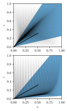
Figure 2: Trajectories of the auxiliary dynamics (48) for different initial conditions ($\kappa=0.4$, $\bar{a}=0.5$, $\hat{\gamma}=0.2$, $\hat{\mu}=0.1$) - $T=1.0$ (top) and $T=0.4$ (bottom). The black vector describes the direction defined by $\hat{w}$ as in Theorem 24, while the shaded area defines the cone that contains all the vectors that would satisfy (56), i.e., all the vectors $\hat{w}$ that define a valid Lyapunov function $V_{l}(w)=\hat{w}^{\top}w$.

Theorem 24.

The positive discrete-time linear system (49) is asymptotically stable if and only if the following condition is satisfied:

$$T^{2}\hat{\mu}\hat{\gamma}-(1-\kappa)(1-(1-T\bar{a})^{\frac{1}{q}})<0,$$ (54)

which holds for any sufficiently small sampling time $T\leq T_{5}\vcentcolon=\frac{\beta(1-\kappa)}{\hat{\mu}}$. Moreover, the function $V_{l}(w)\vcentcolon=\hat{w}^{\top}w$, where

$$\hat{w}=\begin{bmatrix}1\\ \beta\end{bmatrix},\quad\mathrm{with}\quad\beta\vcentcolon=\frac{1}{2}\frac{\bar{a}}{q\hat{\gamma}},$$ (55)

is a Lyapunov function for (48) in $\mathbb{R}_{\geq 0}^{2}$. In order to prove that $\hat{w}^{\top}w$ is a Lyapunov function for (48) it suffices to apply Theorem 23. The system of inequalities

$$-1+(1-T\bar{a})^{\frac{1}{q}}\,+T\hat{\gamma}\,\beta <0,$$ (56)

$$T\hat{\mu}\,+(\kappa-1)\,\beta <0,$$

$$\beta >0$$

admits a solution if

$$T\frac{\hat{\mu}}{1-\kappa}<\beta<\frac{1-(1-T\bar{a})^{\frac{1}{q}}}{T\hat{\gamma}}.$$ (57)

This condition can always be satisfied for a sufficiently small $T$. In fact, it is easy to show that the limits for $T\to 0$ of the upper and lower bounds on $\beta$ are 0 and $\frac{\bar{a}}{q\hat{\gamma}}>0$, respectively, such that, by continuity, there must exist a strictly positive constant $T_{5}$ such that (54) is satisfied for any $T\leq T_{5}$. However, in order to make $\beta$ independent of $T$, we note that, due to convexity, $1-(1-T\bar{a})^{\frac{1}{q}}\geq\frac{\bar{a}}{q}T$ for any $T\geq 0$. Using this lower bound we can simplify the upper bound in (57) as

$$\beta<\frac{\frac{\bar{a}}{q}T}{\hat{\gamma}T}=\frac{\bar{a}}{q\hat{\gamma}}\leq\frac{1-(1-T\bar{a})^{\frac{1}{q}}}{T\hat{\gamma}}.$$ (58)

Choosing $\beta$ to be half of this upper bound, i.e., $\beta\vcentcolon=\frac{1}{2}\frac{\bar{a}}{q\hat{\gamma}}$, we obtain that (57) is satisfied for any $T\leq T_{5}\vcentcolon=\frac{\beta(1-\kappa)}{\hat{\mu}}$, which concludes the proof. ∎

Theorem 24 shows that (exponential) asymptotic stability of the auxiliary dynamics holds under the condition that the sampling time $T$ satisfies inequality (54) for given $\hat{\mu}$, $\bar{a}$, $\hat{\gamma}$, and $\kappa$. Figure 2 illustrates the meaning of Theorem 24 by showing the trajectories of the auxiliary system in a phase plot for fixed values of the parameters $\hat{\mu},\bar{a},\kappa$, and $\hat{\gamma}$, two different values of the sampling time $T$ and for different initial conditions. In the following, we establish the main result of the section by exploiting the Lyapunov decrease established in Theorem 24 for the auxiliary dynamics to construct a Lyapunov function for the combined system-optimizer dynamics (16).

Theorem 25.

Let Assumptions 2, 3, 6, 9, 10, and 13 hold. Then, for any $T\leq\min\{T_{4},T_{5}\}$, the origin is an exponentially asymptotically stable equilibrium with region of attraction $\Sigma$ for the combined system-optimizer dynamics (16). In particular, the function

$$V_{\mathrm{so}}(\xi)\vcentcolon=\hat{w}^{\top}\begin{bmatrix}V(x)^{\frac{1}{q}}\\ \|z-\bar{z}(x)\|\end{bmatrix},$$ (59)

where $\hat{w}$ is defined according to Theorem 24, is a Lyapunov function in $\Sigma$ for the system (16) and the origin $(x,z)=\xi=0$. We can derive an upper bound for $V_{\mathrm{so}}(\xi)$ as follows:

$$V_{\mathrm{so}}(\xi) =V(x)^{\frac{1}{q}}+\beta\|z-\bar{z}(x)\|$$ (60)

$$\leq a_{2}^{\frac{1}{q}}\|x\|+\beta\|z-\bar{z}(x)\|$$

$$\leq a_{2}^{\frac{1}{q}}\|x\|+\beta(\|z\|+\|\bar{z}(x)\|)$$

$$\leq(a_{2}^{\frac{1}{q}}+\sigma\beta)\|x\|+\beta\|z\|$$

$$\leq\underbrace{\max\{a_{2}^{\frac{1}{q}}+\sigma\beta,\beta\}}_{=\vcentcolon\tilde{w}_{2}}\cdot\left(\|x\|+\|z\|\right)$$

$$\leq\tilde{w}_{2}\cdot(\|x\|_{1}+\|z\|_{1})=\tilde{w}_{2}\cdot\|\xi\|_{1}$$

$$\leq\tilde{w}_{2}\sqrt{n_{x}+n_{z}}\cdot\|\xi\|.$$

In order to derive a lower bound, we proceed as follows. Using the reverse triangle inequality and Lipschitz continuity of $\bar{z}(x)$, we obtain

$$V_{\mathrm{so}}(\xi) \geq V(x)^{\frac{1}{q}}+\beta(\|z\|-\sigma\|x\|)$$ (61)

$$\geq a_{1}^{\frac{1}{q}}\|x\|+\beta(\|z\|-\sigma\|x\|)$$

$$=(a_{1}^{\frac{1}{q}}-\beta\sigma)\|x\|+\beta\|z\|.$$

If $a_{1}^{\frac{1}{q}}-\beta\sigma>0$, then we can readily compute a lower bound:

$$V_{\mathrm{so}}(\xi) \geq(a_{1}^{\frac{1}{q}}-\beta\sigma)\|x\|+\beta\|z\|$$ (62)

$$\geq\frac{a_{1}^{\frac{1}{q}}-\beta\sigma}{\sqrt{n_{x}}}\|x\|_{1}+\frac{\beta}{\sqrt{n_{z}}}\|z\|_{1}$$

$$\geq\underbrace{\min\bigg{\{}\frac{a_{1}^{\frac{1}{q}}-\beta\sigma}{\sqrt{n_{x}}},\frac{\beta}{\sqrt{n_{z}}}\bigg{\}}}_{=\vcentcolon\tilde{w}_{1,1}}(\|x\|_{1}+\|z\|_{1})$$

$$\geq\tilde{w}_{1,1}\cdot\|\xi\|.$$

If instead $a_{1}^{\frac{1}{q}}-\beta\sigma\leq 0$, we define the auxiliary lower bound

$$\hat{V}_{\mathrm{so}}(x,z)\vcentcolon=a_{1}^{\frac{1}{q}}\|x\|+\beta\|z-\bar{z}(x)\|.$$ (63)

Since $V_{\mathrm{so}}(\xi)\geq\hat{V}_{\mathrm{so}}(x,z)$, if we can show that $\hat{V}_{\mathrm{so}}(x,z)$ can be lower bounded by a properly constructed function of $z$, we can use this function to lower bound $V_{\mathrm{so}}(\xi)$ too. To this end, we first observe that, since we assumed that $a_{1}^{\frac{1}{q}}-\beta\sigma\leq 0$, for any $x$ such that $\|x\|\leq\frac{1}{\sigma}\|z\|$, we have that

$$\hat{V}_{\mathrm{so}}(x,z) \geq(a_{1}^{\frac{1}{q}}-\beta\sigma)\|x\|+\beta\|z\|$$ (64)

$$\geq\underset{x\,\mathrm{s.t.}\,\|x\|\leq\frac{1}{\sigma}\|z\|}{\min}(a_{1}^{\frac{1}{q}}-\beta\sigma)\|x\|+\beta\|z\|$$

$$\geq\frac{a_{1}^{\frac{1}{q}}}{\sigma}\|z\|,$$

where, for the minimization, we have used the fact that the objective $(a_{1}^{\frac{1}{q}}-\beta\sigma)\|x\|+\beta\|z\|$ is monotonically nonincreasing in $\|x\|$ such that the minimum is attained at the boundary of the interval for $\|x\|=\frac{1}{\sigma}\|z\|$. Similarly, for any $x$ such that $\|x\|\geq\frac{1}{\sigma}\|z\|$, we can use the fact that

$$\hat{V}_{\mathrm{so}}(x,z) =a_{1}^{\frac{1}{q}}\|x\|+\beta\|z-\bar{z}(x)\|\geq a_{1}^{\frac{1}{q}}\|x\|\geq\frac{a_{1}^{\frac{1}{q}}}{\sigma}\|z\|.$$

Hence, we can conclude that

$$V_{\mathrm{so}}(\xi)\geq\hat{V}_{\mathrm{so}}(x,z)\geq\frac{a_{1}^{\frac{1}{q}}}{\sigma}\|z\|$$ (65)

for any $x$. Summing this last inequality and $V_{\mathrm{so}}(\xi)\geq a_{1}^{\frac{1}{q}}\|x\|$, we obtain

$$V_{\mathrm{so}}(\xi) \geq\frac{a_{1}^{\frac{1}{q}}}{2}\|x\|+\frac{a_{1}^{\frac{1}{q}}}{2\sigma}\|z\|$$ (66)

$$\geq\frac{a_{1}^{\frac{1}{q}}}{2\sqrt{n_{x}}}\|x\|_{1}+\frac{a_{1}^{\frac{1}{q}}}{2\sigma\sqrt{n_{z}}}\|z\|_{1}$$

$$\geq\underbrace{\min\bigg{\{}\frac{a_{1}^{\frac{1}{q}}}{2\sqrt{n_{x}}},\frac{a_{1}^{\frac{1}{q}}}{2\sigma\sqrt{n_{z}}}\bigg{\}}}_{=\vcentcolon\tilde{w}_{1,2}}(\|x\|_{1}+\|z\|_{1})$$

$$\geq\tilde{w}_{1,2}\cdot\|\xi\|.$$

Together with (62), we can define

$$\tilde{w}_{1}\vcentcolon=\begin{cases}\tilde{w}_{1,1},\quad\text{if}\quad a_{1}^{\frac{1}{q}}-\beta\sigma>0,\\ \tilde{w}_{1,2},\quad\text{otherwise},\\ \end{cases}$$ (67)

and conclude that $V_{\mathrm{so}}(\xi)\geq\tilde{w}_{1}\cdot\|\xi\|$. Finally, the Lyapunov decrease can be derived. For given $x$ and $z$, let $\epsilon=E(x,z)$ and $\nu=V(x)^{\frac{1}{q}}$. Then the following holds.

$$V_{\mathrm{so}}(\xi_{+})= \,V_{+}(T;x,z)^{\frac{1}{q}}+\beta E_{+}(T;x,z)$$ (68)

$$\stackrel{{\scriptstyle\mathclap{\rm Remark\,\,\ref{rem:upper_bound}}}}{{\leq}} \,\nu_{+}+\beta\epsilon_{+}$$

$$\stackrel{{\scriptstyle\mathclap{\rm Theorem\,\,\ref{thm:ps_stab}}}}{{\leq}} \,\nu+\beta\epsilon-\hat{d}\cdot\|(\nu,\epsilon)\|_{1}$$

$$= \,V(x)^{\frac{1}{q}}+\beta E(x,z)-\hat{d}\cdot\|(\nu,\epsilon)\|_{1}$$

$$= \,V_{\mathrm{so}}(\xi)-\hat{d}\cdot(V(x)^{\frac{1}{q}}+\|z-\bar{z}(x)\|),$$

where we have used the $\ell_{1}$ norm due to the intermediate result in the proof of Theorem 23. Let $\Delta V_{\mathrm{so}}(\xi)\vcentcolon=-\hat{d}\cdot(V(x)^{\frac{1}{q}}+\|z-\bar{z}(x)\|)$ denote the Lyapunov decrease. Using the same procedure used to derive the lower bound for $V_{\mathrm{so}}(\xi)$, we can show that, if $a_{1}^{\frac{1}{q}}-\sigma>0$, we can write

$$\Delta V_{\mathrm{so}}(\xi) \leq-\hat{d}\cdot\left((a_{1}^{\frac{1}{q}}-\sigma)\|x\|+\|z\|\right)$$

$$\leq-\underbrace{\hat{d}\cdot\min\bigg{\{}\frac{a_{1}^{\frac{1}{q}}-\sigma}{\sqrt{n_{x}}},\frac{1}{\sqrt{n_{z}}}\bigg{\}}}_{=\vcentcolon\tilde{w}_{3,1}}(\|x\|_{1}+\|z\|_{1})$$

$$\leq-\tilde{w}_{3,1}\cdot\|\xi\|.$$

Else, if $a_{1}^{\frac{1}{q}}-\sigma\leq 0$, we can obtain the following bound:

$$\Delta V_{\mathrm{so}}(\xi) =-\hat{d}\cdot\left(V(x)^{\frac{1}{q}}+\|z-\bar{z}(x)\|\right)\leq-\frac{\hat{d}a_{1}^{\frac{1}{q}}}{\sigma}\|z\|.$$

Summing this last inequality and $\Delta V_{\mathrm{so}}(\xi)\leq-\hat{d}a_{1}^{\frac{1}{q}}\|x\|$, we obtain

$$\Delta V_{\mathrm{so}}(\xi) \leq-\frac{\hat{d}a_{1}^{\frac{1}{q}}}{2}\left(\|x\|+\frac{1}{\sigma}\|z\|\right)$$

$$\leq-\frac{\hat{d}a_{1}^{\frac{1}{q}}}{2}\left(\frac{1}{\sqrt{n_{x}}}\|x\|_{1}+\frac{1}{\sigma\sqrt{n_{z}}}\|z\|_{1}\right)$$

$$\leq-\underbrace{\frac{\hat{d}a_{1}^{\frac{1}{q}}}{2}\cdot\min\bigg{\{}\frac{1}{\sqrt{n_{x}}},\frac{1}{\sigma\sqrt{n_{z}}}\bigg{\}}}_{=\vcentcolon\tilde{w}_{3,2}}(\|x\|_{1}+\|z\|_{1})$$

$$\leq-\tilde{w}_{3,2}\cdot\|\xi\|.$$

We define

$$\tilde{w}_{3}\vcentcolon=\begin{cases}\tilde{w}_{3,1},\quad\text{if}\quad a_{1}^{\frac{1}{q}}-\sigma>0,\\ \tilde{w}_{3,2},\quad\text{otherwise},\\ \end{cases}$$ (69)

and conclude that $\Delta V_{\mathrm{so}}(\xi)\leq-\tilde{w}_{3}\cdot\|\xi\|$. Hence, we can define the $\mathcal{K}_{\infty}$ functions $\alpha_{\mathrm{so},1}(\|\xi\|)\vcentcolon=\tilde{w}_{1}\cdot\|\xi\|$ and $\alpha_{\mathrm{so},2}(\|\xi\|)\vcentcolon=\tilde{w}_{2}\cdot\|\xi\|$ and the positive definite function $\alpha_{\mathrm{so},3}(\|\xi\|)\vcentcolon=\tilde{w}_{3}\cdot\|\xi\|$, such that

$$\alpha_{\mathrm{so},1}(\|\xi\|)\leq V_{\mathrm{so}}(\xi)\leq\alpha_{\mathrm{so},2}(\|\xi\|)$$ (70)

$$V_{\mathrm{so}}(\xi_{+})-V_{\mathrm{so}}(\xi)\leq-\alpha_{\mathrm{so},3}(\|\xi\|),$$

i.e., $V_{\mathrm{so}}(\xi)$ is a Lyapunov function in $\Sigma$ for the system-optimizer dynamics $\xi_{+}=\Phi(T;\xi)$ and the equilibrium $\xi=0$, for any $T\leq\min\{T_{4},T_{5}\}$. ∎

Theorem 25 shows that, for a sufficiently short sampling time $T$, the system-optimizer dynamics in (15) are asymptotically exponentially stable and that $V_{\text{so}}$ is a Lyapunov function in $\Sigma$. We observe that the obtained Lyapunov function is a positive linear combination of the ideal NMPC Lyapunov function $V$ and the error $\|z-\bar{z}(x)\|$ (which in turn is a Lyapunov function for the error dynamics). Loosely speaking, depending on the value of $\beta$, $V_{\text{so}}$ gives more “importance” to either $V$ (for small values of $\beta$) or $\|z-\bar{z}(x)\|$ (for large values of $\beta$).

In the next section, in order to illustrate Theorem 25, we use a variant of the classical example from [3].

4 Illustrative example

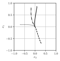
Figure 3: Illustrative example adapted from [3] - closed-loop state trajectories obtained using the approximate feedback policy computed with a single iteration of a Gauss-Newton real-time algorithm.

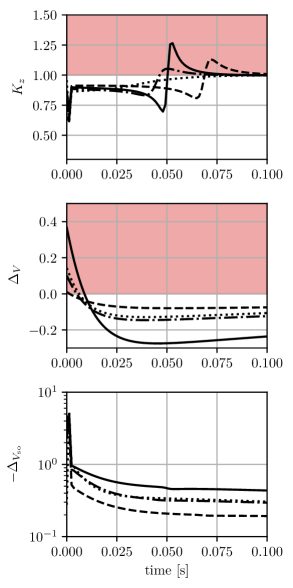
Figure 4: Illustrative example adapted from [3] - although the numerical error and the value function do not necessarily decrease monotonically over time, the Lyapunov function for the combined system-optimizer dynamics $V_{\mathrm{so}}(\xi)$ does decrease.

We regard an optimal control problem of the form in (13) and define the continuous-time dynamics as

$$\phi(x,u)\vcentcolon=\begin{bmatrix}x_{2}+u(\mu+(1-\mu)x_{2})\\ x_{1}+u(\mu-4(1-\mu)x_{2})\end{bmatrix}.$$ (71)

In order to compute an LQR-based terminal cost, the linearized dynamics are defined as

$$A_{\mathrm{c}}\vcentcolon=\frac{\partial\phi}{\partial x}(0,0),\quad B_{\mathrm{c}}\vcentcolon=\frac{\partial\phi}{\partial u}(0,0),$$ (72)

and discretized using exact discretization with piece-wise constant parametrization of the control trajectories:

$$A\vcentcolon=\exp{(A_{\mathrm{c}}T_{\mathrm{d}})},\quad B\vcentcolon=\left(\int_{\tau=0}^{T_{\mathrm{d}}}\exp{(A_{\mathrm{c}}\tau)\mathrm{d}\tau}\right)B_{\mathrm{c}},$$

where $T_{\mathrm{d}}$ denotes the discretization time. We compute the solution $P$ to the discrete-time algebraic Riccati equation

$$P=A^{\top}PA-(A^{\top}PB)(R+B^{\top}PB)^{-1}(B^{\top}PA)+Q,$$

where $Q=0.1\cdot\mathbb{I}_{2}$ and $R=0.1$ such that the cost functionals can be defined as

$$L(x,u)\vcentcolon=x^{\top}Qx+u^{\top}Ru,\quad m(x)\vcentcolon=x^{\top}Px,$$ (73)

and we impose simple bounds on the input $-2\leq u\leq 2$.

We set the prediction horizon $T_{\mathrm{f}}=0.3$ and discretize the resulting continuous-time optimal control problem using direct multiple shooting with $N=5$ shooting nodes. The Euler discretization is used for the cost integral and explicit RK4 is used to discretize the dynamics. In order to solve the resulting discretized optimal control problem, we use the standard RTI approach, with Gauss-Newton iterations and a fixed Levenberg-Marquardt-type term. A single SQP iteration per sampling time is carried out.

In order to compute an estimate for the constants involved in the definition of the Lyapunov function in Theorem 25, we regard six different initial conditions, and control the system using the feedback policy associated with the exact solution to the discretized optimal control problem. For every state $x$ in the obtained trajectories, we evaluate the optimal cost $V(x)$ and the primal-dual optimal solution $\bar{z}(x)$. With these values, we can estimate the constants $a_{1},a_{2},a_{3}$ in Assumption 2, the constant $\tilde{\mu}$ in Assumption 3 and the constant $\sigma$ in Theorem 11. Moreover, for any state visited, we carry out a limited number of iterations of the optimizer in order to estimate the contraction rate $\hat{\kappa}$. Choosing the sampling time $T=0.0012$, we obtain the estimates $\kappa=0.882,\bar{a}=1.157,\hat{\gamma}=70.23$, and $\hat{\mu}=0.360$, such that the parameter involved in the definition of the Lyapunov function for the combined system-optimizer dynamics takes the value $\beta=0.0041$ and we have $T_{5}=0.037\geq T$. All the computations were carried out using CasADi [2] and its interface to Ipopt [17] and the code for the illustrative example is made available at https://github.com/zanellia/nmpc_system_optimizer_lyapunov.

Figure 3 shows the state trajectories obtained controlling the system using the approximate feedback law starting from the selected initial conditions. Figure 4 shows the behavior of $\|z-\bar{z}(x)\|$, $V(x)$ and $V_{\mathrm{so}}(\xi)$ over time through the compact metrics

$$K_{z}\vcentcolon=\frac{\|z_{+}-\bar{z}(x_{+})\|}{\|z-\bar{z}(x)\|},$$ (74)

$$\Delta_{V}\vcentcolon=\frac{V(x_{+})-V(x)}{T_{s}},$$ (75)

$$\Delta_{V_{\text{so}}}\vcentcolon=\frac{V_{\text{so}}(\xi_{+})-V_{\text{so}}(\xi)}{T_{s}}.$$ (76)

In particular, Figure 4 shows that, although the numerical error $\|z-\bar{z}(x)\|$ and the value function does not necessarily decrease over time, the constructed Lyapunov function $V_{\mathrm{so}}(\xi)$ does decrease.

5 Conclusions

In this paper, we presented a novel asymptotic stability results for inexact MPC relying on a limited number of iterations of an optimization algorithm. A class of optimization methods with Q-linearly convergent iterates has been regarded and, under the assumption that the ideal feedback law is stabilizing, we constructed a Lyapunov function for the system-optimizer dynamics. These results extend the attractivity proofs present in the literature which rely instead on the assumption that inequality constraints are either absent or inactive in the attraction region considered. Moreover, with respect to more general results on suboptimal MPC (cf. [15], [12], [1]), we analyzed the coupled system and optimizer dynamics and proved its asymptotic stability.

Future research will investigate how to relax the requirements of Lipschitz continuity of the solution localization $\bar{z}$ and of Q-linear convergence.

Appendix A Proof of Proposition 3.2.16

In the following, we will use the shorthand $u=M_{u,z}z$. First, notice that

$$\psi(t;x,u)=x+\int_{0}^{t}\phi(\psi(\tau;x,u),u)\,\mathrm{d}\tau,\\$$ (77)

and that, due to continuity of $\psi(t;x,u)$ with respect to $t$, for all $x\in X_{\bar{V}}$ and all $z\in\mathcal{B}(\bar{z}(x),r_{z})$, there exists a $T^{\prime}>0$, such that, for all $t\leq T^{\prime}$, we have $\psi(t;x,u)\in X_{\bar{V}}\oplus\mathcal{B}(0,\rho)$.

Using (77) and Assumption 13, we obtain that, for any $x\in X_{\bar{V}}$, all $z\in\mathcal{B}(\bar{z}(x),r_{z})$ and all $T\leq T^{\prime}$, the following holds:

$$\|\psi(T;x,u)-x\| =\Big{\|}\int_{0}^{T}\phi(\psi(\tau;x,u),u)\,\mathrm{d}\tau\Big{\|}$$

$$\leq\int_{0}^{T}\|\phi(\psi(\tau;x,u),u)\|\,\mathrm{d}\tau$$

$$=\int_{0}^{T}\|\phi(\psi(\tau;x,u),u)-\phi(0,0)\|\,\mathrm{d}\tau$$

and, using the fact that $\phi(0,0)=0$,

$$\!\!\!\!\!\!\| \psi(T;x,u)-x\|$$

$$\leq\int_{0}^{T}\!\!\left(L_{\phi,x}\|\psi(\tau;x,u)\|+L_{\phi,u}\|u\|\right)\mathrm{d}\tau$$

$$=\int_{0}^{T}\!\!\left(L_{\phi,x}\|\psi(\tau;x,u)+x-x\|+L_{\phi,u}\|u\|\right)\mathrm{d}\tau$$

$$\leq\int_{0}^{T}\!\!\left(L_{\phi,x}\|\psi(\tau;x,u)-x\|+L_{\phi,u}\|u\|+L_{\phi,x}\|x\|\right)\mathrm{d}\tau$$

$$=\int_{0}^{T}\!\!L_{\phi,x}\|\psi(\tau;x,u)-x\|\,\mathrm{d}\tau$$

$$\quad\quad\quad+T(L_{\phi,u}\|u\|+L_{\phi,x}\|x\|).$$

We can then apply the integral form of Grönwall’s Lemma in order to obtain

$$\|\psi(T;x,u)-x\| \leq Te^{L_{\phi,x}T}(L_{\phi,u}\|u\|+L_{\phi,x}\|x\|)$$

for any $x\in X_{\bar{V}}$ and all $z\in\mathcal{B}(\bar{z}(x),r_{z})$. Similarly, in order to prove the second inequality, we first notice that there must exist a $T^{\prime\prime}>0$ such that, for all $x\in X_{\bar{V}}$, for all $u=M_{u,z}z$ and all $u^{\prime}=M_{u,z}z^{\prime}$ such that $z,z^{\prime}\in\mathcal{B}(\bar{z}(x),r_{z})$ and for all $t\leq T^{\prime\prime}$, we have $\psi(t;x,u),\psi(t;x,u^{\prime})\in X_{\bar{V}}\oplus\mathcal{B}(0,\rho)$. Hence, for any $x\in X_{\bar{V}}$ and all $z,z^{\prime}\in\mathcal{B}(\bar{z}(x),r_{z})$ and all $T\leq T^{\prime\prime}$ we can proceed as follows:

$$\|\psi (T;x,u^{\prime})-\psi(T;x,u)\|$$

$$\leq\int_{0}^{T}\|\phi(\psi(\tau;x,u^{\prime}),u^{\prime})-\phi(\psi(\tau;x,u),u)\|\,\mathrm{d}\tau$$

$$=\int_{0}^{T}\|\phi(\psi(\tau;x,u^{\prime}),u^{\prime})-\phi(\psi(\tau;x,u),u)$$

$$\quad+\phi(\psi(\tau;x,u^{\prime}),u)-\phi(\psi(\tau;x,u^{\prime}),u)\|\,\mathrm{d}\tau$$

$$\leq\int_{0}^{T}\|\phi(\psi(\tau;x,u^{\prime}),u^{\prime})-\phi(\psi(\tau;x,u^{\prime}),u)\|\mathrm{d}\tau$$

$$\quad+\int_{0}^{T}\|\phi(\psi(\tau;x,u),u)-\phi(\psi(\tau;x,u^{\prime}),u)\|\,\mathrm{d}\tau$$

$$\leq TL_{\phi,u}\|u^{\prime}-u\|$$

$$\quad+\int_{0}^{T}L_{\phi,x}\|\psi(\tau;x,u^{\prime})-\psi(\tau;x,u)\|\,\mathrm{d}\tau$$

and, applying Gröonwall’s Lemma, we obtain

$$\|\psi(T;x,u^{\prime})-\psi(T;x,u)\| \leq TL_{\phi,u}e^{TL_{\phi,x}}\|u^{\prime}-u\|.$$

Finally, we pick $T_{1}\vcentcolon=\min\{T^{\prime},T^{\prime\prime}\}$ and define $L_{\psi,x}\vcentcolon=e^{L_{\phi,x}T_{1}}L_{\phi,x}$ and $L_{\psi_{,}u}\vcentcolon=e^{L_{\phi,x}T_{1}}L_{\phi,u}$, such that

$$\|\psi(T;x,u)-x\|\leq T\cdot(L_{\psi,x}\|x\|+L_{\psi,u}\|u\|)$$ (78)

and

$$\|\psi(T;x,u^{\prime})-\psi(T;x,u)\|\leq TL_{\psi,u}\|u^{\prime}-u\|.$$

for any $x\in X_{\bar{V}}$, all $z,z^{\prime}\in\mathcal{B}(\bar{z}(x),r_{z})$ and any $T\leq T_{1}$. ∎

Appendix B Proof of Theorem 3.2.25

It suffices to show that $V_{l}(w)$ is a Lyapunov function for (51) in $\mathbb{R}_{\geq 0}^{n}$. Define $\hat{w}_{\min}\vcentcolon=\underset{i=1,\dots,n}{\min}\,[\,\hat{w}\,]_{i}$ and $\hat{w}_{\max}\vcentcolon=\underset{i=1,\dots,n}{\max}\,[\,\hat{w}\,]_{i}$. The following inequalities hold:

$$\hat{w}^{\top}w\geq\hat{w}_{\min}\cdot\mathbf{1}^{\top}w=\hat{w}_{\min}\cdot\|w\|_{1}\geq\hat{w}_{\min}\cdot\|w\|_{2}$$

and

$$\hat{w}^{\top}w \leq\hat{w}_{\max}\cdot\mathbf{1}^{\top}w$$

$$\leq\hat{w}_{\max}\cdot\|\mathbf{1}\|_{2}\|w\|_{2}$$

$$\leq\sqrt{n}\,\hat{w}_{\max}\cdot\|w\|_{2},$$

which show that there exist $\mathcal{K}_{\infty}$ functions $\alpha_{l,1}(\|w\|)\vcentcolon=\hat{w}_{\min}\cdot\|w\|$ and $\alpha_{l,2}(\|w\|)\vcentcolon=\sqrt{n}\,\hat{w}_{\max}\cdot\|w\|$ such that

$$\alpha_{l,1}(\|w\|)\leq V_{l}(w)\leq\alpha_{l,2}(\|w\|).$$ (79)

Moreover, for any $w>0$, we have that

$$V_{l}(w_{+})-V_{l}(w) =\hat{w}^{\top}Aw-\hat{w}^{\top}w$$ (80)

$$=\hat{w}^{\top}(A-\mathbb{I})\,w$$

$$=w^{\top}(A^{\top}-\mathbb{I})\,\hat{w}$$

$$\leq-\hat{d}\cdot\|w\|_{1}\leq-\hat{d}\cdot\|w\|_{2}.$$

Hence, there exists a positive definite and continuous function $\alpha_{l,3}(\|w\|)\vcentcolon=\hat{d}\cdot\|w\|$ such that, for any $w\geq 0$, the following holds

$$V_{l}(w_{+})-V_{l}(w)\leq-\alpha_{l,3}(\|w\|)$$ (81)

and $\alpha_{l,3}(0)=0$, which concludes the proof. ∎

Remark 26.

Notice that the original Theorem in [10] requires the existence of a strictly positive vector $\hat{w}>0$ such that

$$(A-\mathbb{I})\hat{w}<0.$$ (82)

Although the condition used in Theorem 23 is equivalent to one above, the resulting $\hat{w}$ can only be used to define a Lyapunov function for the dual system $w_{+}=A^{\top}w$.

References

• [1] D. A. Allan, C. N. Bates, M. J. Risbeck, and J. B. Rawlings. On the inherent robustness of optimal and suboptimal nonlinear MPC. Systems & Control Letters, 106:68–78, 2017.
• [2] J. A. E. Andersson, J. Gillis, G. Horn, J. B. Rawlings, and M. Diehl. CasADi: a software framework for nonlinear optimization and optimal control. Mathematical Programming Computation, pages 1–36, 2019.
• [3] H. Chen and F. Allgöwer. A quasi-infinite horizon nonlinear model predictive control scheme with guaranteed stability. Automatica, 34(10):1205–1218, 1998.
• [4] M. Diehl. Real-Time Optimization for Large Scale Nonlinear Processes, volume 920 of Fortschritt-Berichte VDI Reihe 8, Meß-, Steuerungs- und Regelungstechnik. VDI Verlag, Düsseldorf, 2002. PhD Thesis.
• [5] M. Diehl, R. Findeisen, and F. Allgöwer. A stabilizing real-time implementation of nonlinear model predictive control. In L. Biegler, O. Ghattas, M. Heinkenschloss, D. Keyes, and B. van Bloemen Waanders, editors, Real-Time and Online PDE-Constrained Optimization, pages 23–52. SIAM, 2007.
• [6] M. Diehl, R. Findeisen, F. Allgöwer, H. G. Bock, and J. P. Schlöder. Nominal stability of the real-time iteration scheme for nonlinear model predictive control. IEE Proc.-Control Theory Appl., 152(3):296–308, 2005.
• [7] C. Feller and C. Ebenbauer. Relaxed logarithmic barrier function based model predictive control of linear systems. IEEE Transactions on Automatic Control, 62(3):1223–1238, March 2017.
• [8] K. Graichen and A. Kugi. Stability and incremental improvement of suboptimal MPC without terminal constraints. IEEE Transactions on Automatic Control, 55(11):2576–2580, 2010.
• [9] N. H. Josephy. Newton’s method for generalized equations and the PIES energy model. PhD thesis, University of Wisconsin-Madison, 1979.
• [10] T. Kaczorek. The choice of the forms of Lyapunov functions for a positive 2D Roesser model. International Journal of Applied Mathematics and Computer Science, 17(4):471–475, Jan 2008.
• [11] D. Liao-McPherson, M. Nicotra, and I. Kolmanovsky. Time-distributed optimization for real-time model predictive control: Stability, robustness, and constraint satisfaction. Automatica, 117, 2020.
• [12] G. Pannocchia, J. Rawlings, and S. Wright. Conditions under which suboptimal nonlinear MPC is inherently robust. System & Control Letters, 60(9):747–755, 2011.
• [13] J. B. Rawlings, D. Q. Mayne, and M. M. Diehl. Model Predictive Control: Theory, Computation, and Design. Nob Hill, 2nd edition edition, 2017.
• [14] S. M. Robinson. Strongly Regular Generalized Equations. Mathematics of Operations Research, Vol. 5, No. 1 (Feb., 1980), pp. 43-62, 5:43–62, 1980.
• [15] P. O. M. Scokaert, D. Q. Mayne, and J.B. Rawlings. Suboptimal Model Predictive Control (Feasibility Implies Stability). IEEE Transactions on Automatic Control, 44(3):648–654, 1999.
• [16] R. Van Parys and G. Pipeleers. Real-time proximal gradient method for linear MPC. In Proceedings of the European Control Conference (ECC), Lymassol, Cyprus, 2018.
• [17] A. Wächter and L. Biegler. IPOPT - an Interior point optimizer. https://projects.coin-or.org/Ipopt, 2009.
• [18] A. Zanelli, J. Kullick, H. Eldeeb, G. Frison, C. Hackl, and M. Diehl. Continuous control set nonlinear model predictive control of reluctance synchronous machines. IEEE Transactions on Control Systems Technology, pages 1–12, February 2021.