Variety of scaling behaviors in nanocrystalline plasticity

Abstract

We address the question of why larger, high symmetry crystals are mostly weak, ductile and statistically sub-critical, while smaller crystals with the same symmetry are strong, brittle and super-critical. We link it to another question of why intermittent elasto-plastic deformation of sub-micron crystals features highly unusual size sensitivity of scaling exponents. We use a minimal integer-valued automaton model of crystal plasticity to show that with growing variance of quenched disorder, which can serve in this case as a proxy for increasing size, sub-micron crystals undergo a crossover from spin-glass marginality to criticality characterizing the second order brittle-to-ductile (BD) transition. We argue that this crossover is behind the non-universality of scaling exponents observed in physical and numerical experiments. The non-universality emerges only if the quenched disorder is elastically incompatible and it disappears if the disorder is compatible.

I Introduction

Considerable research efforts have been recently focused on the study of mechanical properties of sub-micron crystals Han et al. (2015); Maaß et al. (2012); Mordehai et al. (2011); Papanikolaou et al. (2017); Maaß and Derlet (2018). It was found that the deformation mechanisms, which we habitually associate with dislocation plasticity, change dramatically once the sample size is reduced below the micrometer range. Strength of such crystals was shown to be size-dependent Uchic et al. (2004); Greer et al. (2005); Dimiduk et al. (2006), with stress-strain response exhibiting pronounced intermittency and scale-invariance over a wide range of scales, independently of crystal symmetry  Zaiser (2006); Uchic et al. (2009); Csikor et al. (2007); Friedman et al. (2012); Maass et al. (2015); Ng and Ngan (2008); Brinckmann et al. (2008); Zaiser et al. (2008a). Both measured and computed scaling exponents were shown to feature highly unusual size dependence Papanikolaou et al. (2012); Zhang et al. (2017a).

Moreover, even though plasticity at macroscale is generally associated with ductility, crystal plasticity at sub-micron scales exhibits major stress drops or strain bursts reminiscent of brittle fracture  Cui et al. (2017); Maaß and Derlet (2018); Wang et al. (2012); Chrobak et al. (2011a); Bei et al. (2008a). Brittleness, usually attributed to dislocation-free crystals Broberg (1999), reappears in nano-particles and nano-pillars that seem to be ’breaking plastically’ by generating a large number of globally correlated dislocations Sharma et al. (2018a); Mordehai et al. (2018). The implied system-size events hinder our ability to control plastic deformation at sub-micron scale and compromise the reliable functioning of ultra-small machinery Argon (2013); Csikor et al. (2007); Benzerga (2009); Motz et al. (2009); Uchic et al. (2009).

The peculiar properties of sub-micron crystals can be linked to the scarcity of dislocation sources and easiness of surface annihilation. This limits dislocation storage and inhibits forest hardening, thus reducing dislocation network complexity and promoting highly anisotropic single slip behavior. The lack of obstacles facilitates the collective behavior, which is ultimately behind intermittency and scaling. Rationalization of the crossover from bulk to surface dominated plastic flow has emerged recently as one of the main challenges in crystal plasticity.

To illustrate the full spectrum of plastic responses at sub-micron scale, we decided to characterize them experimentally for a single material. We conducted a set of compression tests on pure Mo sub-micron pillars, choosing intentionally a ’mild’, in the sense of Weiss et al. (2015), BCC crystal. The main qualitative observation was that larger, dislocation-rich sub-micron crystals are weak, ductile, and statistically sub-critical. In contrast, smaller, dislocation-starved crystals are strong, brittle, and statistically super-critical. One of the aims of this paper is to reproduce the observed behavior using a minimal, analytically transparent model.

The intermittent plastic deformation in crystals was modeled previously using molecular dynamics Niiyama and Shimokawa (2015), discrete dislocation dynamics Miguel et al. (2001); Ispánovity et al. (2014); Ovaska et al. (2015); Papanikolaou et al. (2012); Cui et al. (2017), phase field theories Chan et al. (2010) and various meso-scopic approaches Zaiser and Nikitas (2007); Salman and Truskinovsky (2011). The results of different simulations are not fully consistent, suggesting that scaling exponents may be covering a broad range of values Sparks and Maaß (2018); Song et al. (2019); Zhang et al. (2017a) and supporting the idea that micro-plasticity is not a universal critical phenomenon.

Here we show that, rather surprisingly, the use of an oversimplified model of crystal plasticity introduced in Salman and Truskinovsky (2011, 2012a), allows one to reconcile the existing results while dealing with realistic preparations and avoiding ad hoc assumptions. The main step is the reduction of the plastic flow problem to a computationally effective integer-valued discrete automaton. Despite the simplicity of the ensuing dynamical system, one can account in this way for both short-range and long-range elastic interactions, including dislocation nucleation and immobilization. It also allows one to accumulate sufficient statistics, since one can deal in this way with millions of meso-scopic elements and tens of thousands of dislocations.

Our main result is that the non-universality of sub-micron plasticity and the inferred brittleness of ultra-small crystals can be conceptualized as a multi-stage crossover from spin-glass marginality, characteristic of very small, almost defect-free crystals, to the criticality of larger crystals associated with a brittle-to-ductile (BD) transition.

To simulate the size dependence of scaling exponents in small crystals we assumed that, at least in sub-micron range, the decreasing variance of the quenched disorder can serve as a proxy for contracting crystal size. Behind this assumption is the idea that the role of surface annihilation of dislocations can be mimicked by the scarcity of external sources required for dislocation nucleation in the bulk. Essentially, we exploit the fact that in small systems, the conventional dislocation nucleation sources are compromised or even disabled by their closeness to the surface.

Despite the rather prototypical nature of such approach, we were able to capture both, qualitatively and quantitatively, the size dependence observed in our experiments on Mo micro-pillars. Rather remarkably, we reproduced almost exactly the measured value of the critical exponent characterizing the BD transition in such crystals. Along the way, we revealed a fundamental distinction between elastically compatible (local) and elastically incompatible (nonlocal) quenched disorder and showed that the non-universality emerges only if the quenched disorder is ’nonlocal’ and that it disappears if the disorder is ’local’ as, for instance, in the conventional random field Ising model (RFIM) Dahmen and Sethna (1996); Ozawa et al. (2018).

It should be mentioned that some closely related results have been previously obtained in the studies of amorphous glasses, also exhibiting brittleness, yield, intermittency, and the BD transition. However, outside the limit of extremely well-annealed glasses (practically unreachable), the amorphous systems remain fundamentally different from crystals. For instance, the quenched disorder in glasses and granular systems is often rather special as it is revealed by the hierarchical structure of their energy landscapes. More generally, amorphous solids lack long-range order, which is behind crystallographic constraints for plastic slip, and which ultimately ensures orientation dependence of the mechanical response. Most importantly, mobile dislocations, that may nucleate, annihilate and form complex entanglements in crystals, do not exist in amorphous solids Procaccia et al. (2017a); Ozawa et al. (2018); Popović et al. (2018); Shang et al. (2020a). As we show in this paper, the existence of an additional structure in crystalline plasticity, makes their scaling behavior more nuanced.

The rest of the paper is organized as follows. In Section II we present the results of our compression tests on Mo micro-pillars. We then formulate our computational model in Section III. The possibility to use quenched disorder as a proxi for the system size is discussed in detail Section IV. The macroscopic stress-strain response of the system is studied in Section V and in Section VI we quantify the fractal structure of the associated plastic strain fields. The disorder dependence of the statistics of avalanches is analyzed in Section VII. The related distribution of stability measures is discussed in Section VIII. A simple mean field model, building a bridge between our computational results and the macroscopic parameters used in phenomenological models of crystal plasticity, is presented in Section IX. In Section X we compare the results for monotone and oscillatory loading and in Section XI we compare the effects on plastic scaling of ’local’ and ’nonlocal’ quenched disorders. Our main results are summarized in Section XII.

II Experiment

A millimeter-sized Mo single crystal was cut from a well-annealed Mo ingot of a high purity ($>$ 99.99%). The initial dislocation structure inside this BCC crystal was characterized by transmission electron microscopy (TEM), showing straight screw dislocations along $\langle 111\rangle$ directions (Fig. 1(a)), with a density $\rho\approx 1.6\times 10^{12}\;\rm{m}^{2}$ measured by the line-intercept method. According to these data the estimated equidistant dislocation spacing is $l\sim 1/\sqrt{\rho}\approx 790\;\rm{nm}.$

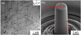
Figure 1: (a) TEM image showing the Grown-in dislocations in the bulk Mo crystal. (b) SEM image of [112]-orientated micro-pillar before compression.

The [112]-oriented Mo pillars with diameters from 500 nm to 1500 nm were fabricated on the electropolished surface of the single bulk crystal by using a Ga-operated focused-ion beam (FIB). The height-to-diameter ratio of the pillars was kept between 2.5:1 and 3:1, and the taper was $\sim 1.7^{\circ}$ (Fig. 1(b)). A nano-indentation system (Hysitron Ti 950) was then used to compress the pillars at room temperature under controlled displacement, with a strain rate of $2\times 10^{-3}\;\rm{s}^{-1}$.

At least four samples were tested for each value of diameter. In Fig. 2 we show the SEM images of the micro-pillars after compression for each size separately. Note the highly anisotropic, single slip plane character of the local plastic deformation pattern in 500 nm and 1000 nm samples: the crystallographically exact slip traces are specifically indicated in Fig. 2 (a,b)). In 1500 nm crystals the plastic flow becomes more isotropic showing even locally a multi-slip deformation pattern.

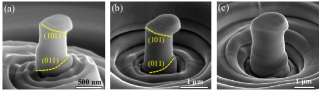
Figure 2: SEM images of [112]-orientated micro-pillars after compression: (a) 500 nm, (b) 1000 nm and (c) 1500 nm. The marked slip traces in (a) and (b) indicate the locally single-slip nature of the plastic flow in 500 nm and 1000 nm crystals.

In Fig. 3(a), we juxtaposed the stress-strain curves for Mo pillars with diameters from 500 nm to 1500 nm, all showing a characteristic set of abrupt discontinuities. For the chosen pillar orientation, the slip systems with maximum Schmidt factor $S$ are (101) $\langle\overline{1}11\rangle$ and (011) $\langle 1\overline{1}1\rangle$. Accordingly, after deformation, we observed the most significant plasticity on the planes $\{110\}$.

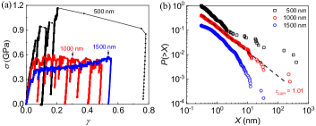
Figure 3: Compression tests on pure Mo sub-micron pillars: (a) stress - strain curves (shear); (b) cumulative distribution of plastic displacements $X$ detected over the entire loading process; here $\tau_{cum}=\tau_{in}-1$ where $\tau_{in}$ is the stress integrated exponent.

The complex configuration of the observed jumps on the stress-strain plane can be explained by the delayed instrumental response during rapid plastic deformation, see Zhang et al. (2017a) for more details. Here we only briefly mention that the mechanical loading in such experiments is performed through an auto-regulation system with PID feedback. The loading device adjusts dynamically, and in the case of an avalanche, it usually does not have enough time to respond. As a result, we observe displacement jumps at an almost constant force.

The plastic displacement jumps were determined from the recorded force-displacement data using the post-processing methodology developed in Zhang et al. (2017a). The size of dislocation avalanche was associated with the plastic displacement $X=D_{e}-D_{s}+(F_{s}-F_{e})/K_{p}$, where $D_{s}$ and $D_{e}$ are the measured displacement at the beginning of the jump and at its end, $F_{s}$ and $F_{e}$ are the corresponding values of the force, and $K_{p}$ is the independently measured stiffness of the pillar. The computed value of $X$ is expected to scale with the total distance covered by all mobile dislocations during an avalanche Maaß et al. (2013).

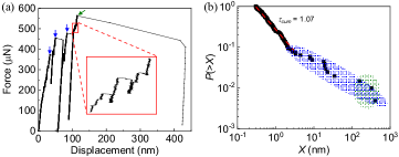
Figure 4: Representative force-plastic displacement curve (a) and cumulative probability distribution of plastic displacements $X$ detected over the entire deformation path (b) for the Mo pillars with 500 nm diameter.

The cumulative probability distributions $P(X)$ are shown in Fig. 3(b) for all three sample sizes. A statistical analysis of these distributions, which involved the comparison of the p-values and the likelihood ratios, allows us to conclude that: (i) for 500 nm Mo micro-pillars the outliers observed above $X\approx 3\ nm$ are statistically significant and indicate super-criticality; (ii) for 1000 nm Mo micro-pillars, the power-law distribution is strongly supported; (iii) for 1500 nm Mo micro-pillars, both, the power-law with a cut-off and the log-normal distribution are more favorable than the power-law distribution, but the log-normal distribution is more likely.

In Fig. 4(a), we illustrate the origin of the characteristic peak which is typical for the super-critical response Sornette and Ouillon (2012), see the green ellipse in Fig. 4(a) based on the data for four micro-pillars with the same diameter 500 nm. One of these large events corresponds to the system size avalanche which is marked by the green arrow in Fig. 4 (a) and signaling the ‘global failure’ of the sample. The mid-sized bursts marked in Fig. 4(b) in violet correspond to brittle events indicated in Fig. 4(a) by violet arrows. The remaining small events show at least one decade of a power-law behavior with the cumulative exponent $\tau_{cum}\approx 1.07$. The coexistence of a power-law range at small scales, with a separate peak representing system size events, is typical for spinodal criticality da Rocha and Truskinovsky (2020).

We note that the statistical super-criticality of nano-scale samples was not emphasized in the previous studies of the scaling in sub-micron crystals Zaiser et al. (2008b); Cui et al. (2020a); Sparks et al. (2019). Instead, it was stressed that in almost pure crystals with negligible number of dislocations, for instance, in sub-micron and nano-particles Wang et al. (2012); Chrobak et al. (2011b), nanowires Lu et al. (2011), or sub-micron pillars Bei et al. (2008b); Issa et al. (2015), the plastic deformation culminates with the formation of a system size slip band. As we show below, both phenomena have the same origin and can be ultimately linked to dislocation starvation Greer and Nix (2006).

III Modeling

To simulate the observed behavior of micro-pillars, we use the minimal model first introduced in Salman and Truskinovsky (2011).

We can assume that the displacement field is scalar because the plastic flow of sufficiently small micro-pillars is mainly single-slip independently of the underlying crystal symmetry and even in the case of multi-slip orientation. Due to a limited number of available dislocation sources within the confined volume, the first activated slip plane dominates and prevents other slip planes from getting involved. In this situation, the usual frustration leading to hardening, can be avoided considering the absence of dislocation cross-slip and facile annihilation at a free surface. While any adequate crystal plasticity model would effectively reduce to our constrained single-slip theory in a sufficiently small system, it should, of course, allow for multi-slip flow to take over at larger sample sizes.

We assume that the crystal is oriented for a single slip along the only available slip direction. It is modeled as an $N\times N$ square lattice with the meso-scopic spacing normalized to unity. The deformation of the crystal is given by the displacements of the vertices of the mesoscopic elements, $\vec{u}_{i,j}=(u^{x}_{i,j},u^{y}_{i,j})$, where $i,j=1,2,\dots,N$.

In view of our single slip assumption we only allow displacements in the horizontal direction by setting $u^{y}_{i,j}\equiv 0$. We can then introduce the notation $u_{i,j}\equiv u^{x}_{i,j}$. In the presence of a kinematic constraint the strain tensor can be reduced to two fields: a longitudinal strain, $\zeta_{i,j}=u_{i+1,j}-u_{i,j},$ which is a linear, non-order parameter variable, and a shear strain $\xi_{i,j}=u_{i,j+1}-u_{i,j},$ which is a nonlinear, order parameter type variable, given that plastic slip originates from multi-well nature of lattice potential.

We write the dimensionless energy of the system in the form Salman and Truskinovsky (2011)

$$\Phi=\sum_{i,j}f(\zeta_{i,j},\xi_{i,j}),$$ (1)

where

$$f(\zeta,\xi)=(K/2)\zeta^{2}+f_{0}(\xi)$$ (2)

is the energy of a single (meso-scopic) element. To account for the lattice periodicity we assume that $f_{0}(\xi)=f_{0}(\xi+n),$ where $n\in\mathbb{Z}$ is an integer-valued slip. Moreover, for analytical transparency we assume that the periodic energy density $f_{0}$ is piece-wise quadratic

$$f_{0}(\xi_{i,j})=(1/2)(\xi_{i,j}-d_{i,j}(\xi))^{2},$$ (3)

Here the plastic slip $d$ is represented by an integer nearest to $\xi$ so that $d_{i,j}(\xi)=\lfloor\xi_{i,j}\rceil.$

The obtained model depends on a single dimensionless parameter $K$which mimics the ratios of elastic constants $(C_{11}-C_{12})/(4C_{44})$ or $C_{11}/C_{66}$. It describes the coupling between mesoscopic elements that carry different values of $\xi$. In the limits $K\to 0,\infty$ we obtain solvable 1D models with mean field type interaction Puglisi and Truskinovsky (2005); Salman and Truskinovsky (2012a). At $K\neq 0$ the model reproduces Eshelby-type propagator and therefore captures crucial effects of long range interactions induced by elastic compatibility, see more about this in Section XI. In our numerical experiments we assumed that $K=2$ which represents a typical value for metallic crystals.

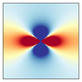
Figure 5: The real-space representation of the dipole Fourier kernel $\hat{L}(\mathbb{q})$. Coloring: blue - negative, red - positive.

The model can be reduced to a discrete automaton because the elastic problem

$$\partial\Phi/\partial u_{i,j}=0$$ (4)

can be solved analytically if the integer-valued field $d$ is known Salman and Truskinovsky (2011). The associated equilibrium equations in the bulk, written terms of the displacement field $u_{i,j}$, read

$$K{}(u_{i+1,j}+u_{i-1,j}-2u_{i,j})+(u_{i,j+1}+u_{i,j-1}-2u_{i,j})\\ -(d_{i,j}-d_{i,j-1})=0.$$ (5)

The whole system can be written in matrix form $\textbf{M}u=b,$ where M is a pentadiagonal matrix and $b$ is a vector of size $N\times N$ incorporating the boundary conditions and the field $d$. The problem then reduces to a simple matrix inversion.

We assume periodic boundary conditions in the horizontal direction $u_{1,j}=u_{N+1,j}$. The hard device type loading will be applied through the boundary condition in the vertical direction $u_{i,N+1}=u_{i,1}+\gamma$, where $\gamma$ is the control parameter. Periodicity is assumed to allow for the fully explicit inversion of the matrix M. Indeed, we can then use the spectral approach based on the Fourier transform

$$\hat{x}(\mathbb{q})=N^{-2}\sum_{ab}x_{a,b}e^{-{i}\mathbb{q}\mathbb{r}}$$ (6)

with $\mathbb{r}=(a,b)$ and $\mathbb{q}=(2\pi k/N,2\pi l/N)$. In Fourier space the solution of our linear problem is straightforward and we can obtain an explicit representation for the equilibrium shear strain

$$\hat{\xi}(\mathbb{q})=\gamma\delta(\mathbb{q})+\hat{L}(\mathbb{q})\hat{d}(\mathbb{q}),$$ (7)

where we recall that $\gamma=\langle\xi\rangle$ is the measure of the imposed affine deformation. The sign-indefinite Eshelby-type kernel with $r^{-2}$ far field asymptotics

$$\hat{L}(\mathbb{q})=\frac{\sin^{2}(q_{y}/2)}{K\sin^{2}(q_{x}/2)+\sin^{2}(q_{y}/2)},$$ (8)

is illustrated in the physical space in Fig.5. Its dipolar structure reflects the scalar nature of our model; the more conventional quadruple structure of the stress propagator is a feature of isotropic elasticity, while here we deal with extremely anisotropic limit Picard et al. (2004); Tyukodi et al. (2016).

To illustrate dislocation nucleation in this model we show in Fig. 6 two dislocations of opposite signs forming a 2D topologically neutral ’loop’. The far-field asymptotics around each of the dislocations agrees with the classical continuum prediction $r^{-1}$, while inside the cores, located around the units where $d_{i+1,j}-d_{i,j}\neq 0$, the stress remains finite due to the strongly discrete nature of our theory.

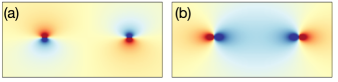
Figure 6: Stress field produced by a pair of dislocations of different signs created using a distribution of plastic slip ($d$ field) which vanishes everywhere except in the one element-wide 80 lattice spacings long segment. (a) Axial stress field $\sigma_{xx}$; (b) Shear stress field $\sigma_{xy}$. Coloring indicates the level of stress: blue - negative, red - positive.

Since we know how to update the elastic fields, we can formulate the quasi-static athermal dynamics in the form of a discrete automaton for the integer-valued field $d$. We start with the unloaded ($\gamma=0$) and dislocation-free state ($d_{i,j}\equiv 0$). We then advance the loading parameter $\gamma$ and compute (predict) the elastic field $u_{i,j}$ while keeping the field $d_{i,j}$ fixed. The knowledge of the shear strain field $\xi_{i,j}$ allows us to update (correct) the plastic strain field using the relation $d=\lfloor\xi\rceil$; the update takes place when the boundary of the energy well is reached by at least one of the mesoscopic elements. Then an avalanche occurs while we use synchronous dynamics for the updates of $d_{i,j}$. We repeat the prediction-correction steps at a given $\gamma$ till the corrections stop changing the field $d_{i,j}$ and the system stabilizes in a new equilibrium state. As the stress in this state is globally below the threshold, we can start a new search for the increment of $\delta\gamma$ that destabilizes at least one unit. As soon as such an element with $d_{i,j}\neq\lfloor\xi\rceil$ is obtained we apply our relaxation protocol again, initiating another avalanche. When avalanche finishes, the variation of $\gamma$ resumes.

IV Incompatible disorder

Given our periodic boundary conditions, we effectively consider an infinite crystal and our parameter $N$ cannot be associated with the crystal size $L$. To model the physical size effect, we would have to deal with more complex boundary conditions compatible with, say, surface dislocation nucleation and the formation of one-legged Frank-Reed loops. Without such major modifications of the model, we can study the size effect only indirectly and we propose to use the strength of quenched disorder as a way to differentiate between sub-micron crystal sizes.

To justify this approach we first note that instead of $L$ one should use a dimensionless parameter which we can always write as

$$R=L/l,$$ (9)

where $l$ is some appropriately chosen internal length scale and without loss of generality we can write $l\sim Gb/\sigma_{th}$, where $G$ is the shear modulus, $b$ is the Burgers vector, and $\sigma_{th}$ is the internal stress threshold.

Following (Zhang et al., 2017a), we identify this threshold with the pinning (immobilization) stress. The distinctly brittle regime for semi-pure crystal would then correspond to small $\sigma_{th}$ due to negligible number of obstacles ensuring that $R\ll 1$. Given that in our Mo samples the spacing of immobile dislocations $l\sim 790$ nm, brittleness of 500 nm pillars would be in a basic agreement with such criterion. In the strongly ductile regime we should have $R\gg 1$, which is close to being the case for our 1500 nm pillars. Dislocation interaction with obstacles becomes relevant when $R\sim 1$ which is the case for our 1000 nm pillars, see Fig. 1.

The threshold $\sigma_{th}$ naturally depends on the presence of the pinning obstacles and, in general Zhang et al. (2017a), increases with the variance of quenched disorder imitating such obstacles. More specifically, the decrease of $\sigma_{th}$ can be achieved by making the disorder more narrow which can be viewed as the way to eliminate particularly strong obstacles. In this way, instead of decreasing $L$ we can increase $l$, which should be as effective in moving from the brittle regime, where $R\ll 1$, to the ductile regime, where $R\gg 1$. In other words, instead of exploring directly the dominance of surface effects one can exploit the indirect effect that in smaller systems there are fewer strong obstacles that can serve, for instance, as dislocation nucleation sites because the existing ones are compromised or even disabled by their closeness to the surfaces.

It has to be mentioned, however, that our association of the variance of disorder with crystal size is exclusively targeting systems without bulk criticality, as in the case of Mo crystals. One can, in principle, manufacture small crystals with strong (dense) quenched disorder Zhang et al. (2017a) or grow almost pure large crystals with very weak (sparse) quenched disorder Weiss (2019). In general, both quenched disorder and the crystal size would affect brittleness, even though to grow almost defect free crystals (without solutes, precipitates and dislocations), is almost impossible except in case of extremely small sizes (nano-particles).

Our crucial assumption allows one to study the size effect without actually changing the size of the computational system while varying instead the strength of the quenched disorder. Here by disorder we mean first of all inclusions such as solute atoms.

It can be also impurity atoms or even vacancies (or voids) resulting from the motions of dislocation jogs Deschamps et al. (2012). It will be important, however, that such disorder is elastically incompatible producing long-range effects as, for instance, in the case of local volumetric changes.

To account for such disorder in the most simple linear form, we can add to the energy density an additional term proportional to the non-order parameter variable $\zeta$ obtaining

$$f(\xi_{i,j},\zeta_{i,j})=\frac{K}{2}\zeta_{i,j}^{2}+\frac{1}{2}(\xi_{i,j}-d_{i,j}(\xi))^{2}-h_{i,j}\zeta_{i,j}.$$ (10)

Here the random coefficients $h_{i,j}$, drawn independently in each lattice point from Gaussian distribution with variance $\delta$

$$p(r)=(2\pi\delta^{2})^{-1/2}\exp{(-r^{2}/(2\delta^{2}))},$$ (11)

mimic incompatible lattice pre-stress which acts on the order parameter variable $\xi$ only indirectly.

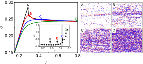
Figure 7: The effect of disorder on the average strain-stress curves in simple shear tests. Inset shows the yield strain $\gamma_{y}$ (points A, B, C, D); the gray strip schematically marks the BD transition. The zoom on the ’after yield’ dislocation configurations is shown in the right column where the total number of dislocations is 782 (in A), 2600 (in B), 5220 (in C) and 8862 (in D). The dislocations with positive and negative Burgers vector are marked by red and blue. Parameters: $K=2,N=1024$.

In the presence of quenched disorder $h$, the strain fields take the form

$$\hat{\xi}(\mathbb{q})=\gamma\delta(\mathbb{q})+\frac{\hat{s}_{y}^{+}(\mathbb{q})[\hat{s}_{x}^{-}(\mathbb{q})\hat{h}(\mathbb{q})+\hat{s}_{y}^{-}(\mathbb{q})\hat{d}\mathbb{(}\mathbb{q})]}{2K[\cos(q_{x})-1]+2[\cos(q_{y})-1]},$$ (12)

$$\hat{\zeta}(\mathbb{q})=\frac{\hat{s}_{x}^{+}(\mathbb{q})[\hat{s}_{x}^{-}(\mathbb{q})\hat{h}(\mathbb{q})+\hat{s}_{y}^{-}(\mathbb{q})\hat{d}\mathbb{(}\mathbb{q})]}{2K[\cos(q_{x})-1]+2[\cos(q_{y})-1]},$$ (13)

where

$$\hat{s}_{a}^{\mp}(\mathbb{q})=\pm[1-\cos(q_{a})\pm i\sin(q_{a})]$$ (14)

for $a=x,y$. We can also rewrite (12) as

$$\hat{\xi}(\mathbb{q})=\gamma\delta(\mathbb{q})+\hat{L}(\mathbb{q})\hat{d}(\mathbb{q})+\hat{L}_{h}(\mathbb{q})\hat{h}(\mathbb{q}),$$ (15)

where

$$\hat{L}_{h}(\mathbb{q})=\frac{\sin(q_{x}/2)\sin(q_{y}/2)(\cos(\frac{q_{x}-q_{y}}{2})-i\sin(\frac{q_{x}-q_{y}}{2}))}{K\sin^{2}(q_{x}/2)+\sin^{2}(q_{y}/2)}$$ (16)

is a distorted Eshelby propagator (8) maintaining, however, its sign-indefiniteness and the decay rate $1/r^{2}$.

V Stress-strain response

Starting with a dislocation-free crystal ($d\equiv 0$) we now drive the system quasistatically using the athermal quasi-static protocol described above Puglisi and Truskinovsky (2005); Maloney and Lemaître (2006). The obtained results are then averaged over $1003000$ realizations of the quenched disorder.

In Fig. 7, we illustrate the average stress-strain relations $\sigma(\gamma)=d\Phi/d\gamma,$ where the stress was averaged over the strain interval $\sim 10^{-4}$. At each value of disorder strength $\delta$ the stress-strain curve exhibits a maximum which we conditionally identify with the yield point. Four of such points are shown in Fig. 7: $A,B,C,D$. The corresponding yield strain is denoted by $\gamma_{y}$ and its dependence on disorder is shown in the inset where the states $A,B,C,D$ are also indicated. The zoom on the ’after yield’ dislocation configurations in these states is shown in the right column.

For weak disorder, $\delta\leq 0.3$, mimicking small, almost pure crystals, yielding is abrupt and brittle, accompanied by a macroscopic stress drop at the yield point and robust strain localization within a formation of a shear band (regime $A$). With increased disorder (regime $B$), the first order phase transition eventually terminates at a critical point located around $\delta\sim 0.42$ (regime $C$), see Ozawa et al. (2018); Popović et al. (2018) for similar behavior in amorphous plasticity. At even stronger disorder, $\delta\geq 0.5$, representing bulk samples, yielding is gradual and plasticity is ductile with slip uniformly distributed over the whole crystal (regime $D$).

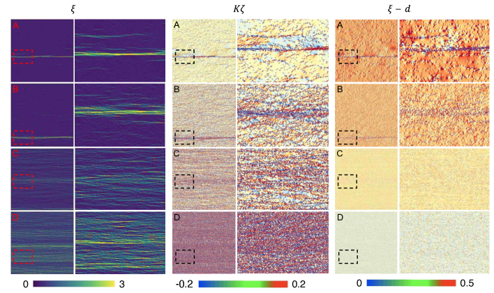
Figure 8: After yield spatial patterns: shear strain $\xi$, longitudinal stress $\sigma_{xx}=\text{d}f/\text{d}\zeta$ and shear stress $\sigma_{xy}=\text{d}f/\text{d}\xi$ in the reference coordinates. Strength of disorder: $\delta=0.28$ (A), $\delta=0.36$ (B), $\delta=0.42$ (C) and $\delta=0.46$ (D). Zoomed views of the marked areas are shown in parallel columns.

In Fig. 8, we show the shear strain, axial stress field and shear stress patterns for samples with disorder strength marked by the letters $A,B,C,D$. In these images, the affine component of the fields was subtracted. We also present enlargement of the marked out windows.

When the disorder is weak (regime $A$), the shear band features a crack-like arrangement of dislocations. Outside the band, the dislocations distribution is relatively uniform, although one can trace few incipient shear pre-bands. As the strength of the disorder increases (regime $B$), the dislocation density inside the shear band diminishes and it becomes progressively broader. One can interpret this broadening as an outside propagation of the shear band boundaries. In the regime $C$, we lose a singular band which is replaced by a diffuse network of interconnected pre-bands which fill the whole domain. Finally, in the ductile phase, regime $D$, no coherent pattern is apparent as we see dislocation activity all over the domain. Note that the overall delocalization of the plastic flow, which we observed experimentally while increasing $L$, is recovered here as we increase $\delta$.

Note, however, that the agreement between this oversimplified theory and the experiment cannot be complete. For instance, in our physical experiments with sub-micron pillars, we observed repeated almost-yielding events. During such events dislocations could always annihilate on free surfaces, which was bringing the crystal into the dislocation starvation state over and over again Wang et al. (2012). Instead, in our computer experiments, where we used periodic boundary conditions, such resetting did not happen because the crystal could form system-size slip bands with high dislocation density. Therefore, for each realization of disorder instead of several large bursts, we observed a single catastrophic one.

VI Spatial complexity

As we see plastic flow proceeds through incessant mechanical destabilization and re-accomodation of dislocational microstructures. Due to the presence of long-range elastic interactions, these microstructures are not random and to reveal the nature of the implicit correlations, we performed a multi-fractal analysis of the field $d_{i,j}$. Originally developed in the studies of fluid turbulence, such analysis has become a powerful tool of quantifying the degree of clustering Paladin and Vulpiani (1987); Mandelbrot (1989); Meneveau and Sreenivasan (1991); Lopes and Betrouni (2009).

Multifractals were introduced to study the distribution of a scalar quantity represented by a measure (usually density, but in our case, plastic strain field). The effect to capture is that local singularities of different strengths are distributed on sets with different fractal dimensions denoted by $D_{q}$. The first of those dimensions $D_{0}$ is the fractal dimension of the geometrical support of the measure. As $q$ increases, the dimensions $D_{q}$ become more and more controlled by the most densely filled domains. An increasing difference between $D_{0}$ and $D_{q}$ with $q>0$ reveals an increasingly multi-scale nature of the distribution.

To compute the dimensions $D_{q}$ in our case we need to cover the deformed lattice with a regular array of boxes of size $L_{b}$ and sum plastic strain in the $m^{th}$ box to obtain $\mathcal{M}_{m}(L_{b})=\sum d$, where the sum is taken over the mesoscopic units covered by a given box. Then, the density of plastic strain associated with the $m^{th}$ box is

$$p_{m}(L_{b})=\frac{\mathcal{M}_{m}(L_{b})}{\sum_{k=1}^{n\left(L_{b}\right)}\mathcal{M}_{k}(L_{b})},$$ (17)

where $n(L_{b})$ is the number of boxes covering the lattice. The moments of order $q$ of this density distribution are

$$M_{q}(L_{b})=\sum_{m=1}^{n(L_{b})}p_{m}^{q}(L_{b}).$$ (18)

If the deformation pattern is self-similar, we should observe the scaling

$$M_{q}(L_{b})\sim L_{b}^{(q-1)D_{q}},$$ (19)

which defines the dimensions $D_{q}$. The singular value $D_{1}$ can be defined as the proportionality coefficient between $\sum_{m}^{n(L_{b})}{p_{m}\log(p_{m})}$ and $\log(L_{b})$, and then $D_{q}\rightarrow D_{1}$ as $q\rightarrow 1$  Weiss (2001); Lebyodkin and Lebedkina (2006).

We computed the dimensions $D_{q}$ at a particular value of the loading parameter $\gamma=0.8$, where the steady flow conditions have already been achieved for all representative values of disorder $\delta$. Our results, summarized in Fig. 9, clearly show the anticipated scaling along several decades till the cut-off scale $L_{b}^{\ast}(\delta)$. It characterizes the spacing of the slip traces, when disorder is weak, and the spacing of the strong dislocation locks, when disorder is strong. The absence of the cut-off at $\delta=0.42$ suggests the emergence of a scale-free hierarchical micro-structure.

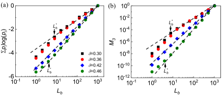
Figure 9: Multifractal analysis of plastic strain patterns for the strain $\gamma=0.8$. (a) $\sum{p_{i}\log(p_{i})}$ (“$M_{1}$”) and (b) $M_{3}$ as a function of box size $L_{b}$.

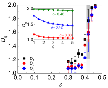
Figure 10: Disorder dependence of the fractal measures $D_{q}$ at $\gamma=0.8$; inset reveals multi-fractality at critical disorder. The gray strip schematically marks the BD transition.

In Fig. 10, we show the disorder dependence of the fractal dimensions $D_{q}$. For weak disorder $D_{q}\sim 1$ for all $q\geq 1$ which signals an extreme localization. At the BD transition the functions $D_{q}$ jump towards the value $\sim 2.0$, which indicates that the strain pattern becomes homogeneous. With the narrow range of disorder strengths $\delta\sim 0.42$ we can associate the emergence of a turbulence-type multi-fractal pattern with $D_{1}>D_{2}>D_{3}>...$. Regions of maximum plastic strain spatially cluster on a set with fractal dimension $\sim 3/2$, which is also characteristic of some other scale-free systems Salerno and Robbins (2013); Gimbert et al. (2013).

VII Avalanche statistics

Both physical and numerical experiments reveal that quasistatically driven crystals deform intermittently via avalanches reflecting destruction and rebuilding of dislocation structures. To perform a quantitative comparison of the two types of experiment we use our observation that in the automaton model the energy $E$, released during an avalanche, scales with the cumulative distance covered by the concurrently moving dislocations. The distribution $p(E)$ computed in numerical experiment will then be the analog of the experimentally measured distribution $p(X)$.

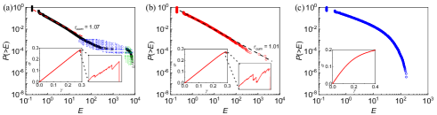
Figure 11: Cumulative probability distributions of pre-yield avalanches at $\delta=0.28$(a), $\delta=0.32$(b), $\delta=0.7$(c); to be compared with the data for 500 nm, 1000 nm and 1500 nm Mo samples shown in Fig. 3(b). Averaging was performed over 100 realizations of disorder; insets show the stress strain curves for a particular realization of disorder.

In Fig. 11 we present the three main types of cumulative distributions $P(>E)$ that emerged in our numerical experiments. Comparison with Fig. 3(b) shows that they reproduce rather faithfully all three types of the distributions $P(>X)$ recorded experimentally. Thus, at small disorder strength, our computational model captures the experimentally observed coexistence of characteristic bursts (SNAP events) with power-law distributed small avalanches observed in 500 nm crystals and, moreover, predicts a realistic value of the experimentally measured exponent, see Fig. 11(a). With increasing disorder the numerically obtained distribution acquires a power-law structure, see Fig. 11(b), with the same exponent as in our data obtained from 1000 nm samples, see Fig. 3(b). At even larger strength of disorder we observe in our numerics the emergence of subcritical statistics, see Fig. 11(c). Therefore, the model captures the observed behavior of 1500 nm samples dominated by largely uncorrelated POP events, see Fig. 3(b). The obtained agreement suggests that we are dealing here with very robust features of the system that are immune to structural details and indifferent to numerical values of parameters. Our results also strongly suggest that the size effect in micro-pillars can be indeed successfully modeled by varying the strength of quenched disorder.

We now turn to the study of the fine details of the disorder-induced crossover phenomena that are not readily accessible in physical experiments. To this end, we approximate at each level of disorder the computed stress-resolved distributions for the released energy $E$ by the scaling relations $p(E)\sim E^{-\tau}\exp(-E/E_{c})$ and extract the disorder-dependent exponents $\tau$ using the maximum likelihood method Clauset et al. (2009). A clear advantage of the numerical experiment, where we could generate at least $3\times 10^{6}$ events for each value of the exponent, is the quality of the statistics.

In Fig. 12(a) we show the obtained continuous functions $\tau(\delta)$ representing pre- and post-yield exponents; the associated strain-resolved distributions are illustrated in Fig. 12(b,c).

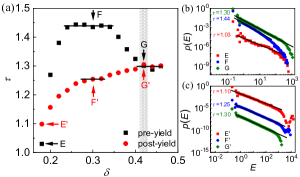
Figure 12: (a) Disorder dependence of the stress-resolved scaling exponent $\tau$ for immediately pre-yield and post-yield regimes; (b,c) corresponding avalanche distributions for more than 100 realizations. The gray strip schematically marks the BD transition.

When the disorder is weak ($\delta\sim 0.2$), the pre- and post-yield exponents take almost the same value $\tau\sim 1$ (points $E$ and $E^{\prime}$ in Fig. 12(a)). In such regimes, where $R<1$, homogeneously nucleated dislocations are free to self-organize under the influence of long-range elastic forces Lehtinen et al. (2016); Mordehai et al. (2018) and the formation of a shear band only mildly affects global dislocation dynamics. The value of the exponent $\tau\sim 1$ presents a signature of archetypically ’wild’ plasticity in the sense of Weiss et al. (2015).

The exponent $\tau=1$ has previously emerged in a fully analytical mean field theory of spin glasses where it was associated with marginal stability Pázmándi et al. (1999); Franz and Spigler (2017). Based on this analogy one can argue that around $\delta\sim 0.2$ our system generates sufficient self-induced disorder to undergo a transition from stable (elastic) to marginally stable (or ’glassy’ ) state whose phase space has a hierarchical (ultrametric) organization Berthier et al. (2019). Such transition usually produces an almost gap-less excitation spectrum Müller and Wyart (2015) which we indeed see emerging in our system, see Section VIII. The analogy with spin-glasses can be linked to the fact that during yielding transition, the system effectively deals with only two neighboring energy wells of the infinitely periodic local energy landscape Pérez-Reche et al. (2008).

The exponent $\tau=1$ was also obtained numerically in the studies of quasi-elastic regimes in structural glasses Tyukodi et al. (2019); Ferrero and Jagla (2019a); Shang et al. (2020a). It was also found to characterize dense amorphous packings and, therefore, can be associated with the concept of jamming. In particular, the avalanche exponent $\tau=1$ is predicted by the fully analytical mean field theory for jammed packings Franz and Spigler (2017).

As we have already mentioned, the fact that the post-yield avalanche distribution in these regimes is super-critical, see, for instance, our data for the 500 nm Mo crystals shown in Fig. 3(b) and Fig. 4(b), is often not explicitly indicated Zaiser et al. (2008a); Cui et al. (2020b); Sparks et al. (2019) even though it is well known that almost pure nano- and micro-crystals always deform with a system size dislocational avalanche Wang et al. (2012); Chrobak et al. (2011a); Lu et al. (2011); Bei et al. (2008a). The super-criticality is also suppressed by the neglect of dislocation nucleation in DDD simulations, even though the exponent $\tau\sim 1$ emerges in such models when they rely on the assumption of single slip plasticity and neglect disorder, e.g. Ispánovity et al. (2014). In fact, the authors of these studies have already linked such regimes with both dislocation jamming and self-induced glassiness Ovaska et al. (2015); Zhang et al. (2016); Lehtinen et al. (2016); Ruscher and Rottler (2019).

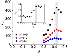
Figure 13: The divergence of the cut-off size in the pre-yield regime around the critical value of disorder $\delta\sim 0.42$. Inset shows the behavior of the fractal dimension $d_{f}$; the gray strip schematically marks the BD transition.

At the intermediate disorder range, where $0.25<\delta<0.35$, we observe a gap opening between the values of pre- and post-yield exponents (regimes $F$ and $F^{\prime}$ in Fig. 12(a)). In view of the progressive rounding of the stress-strain curve near the strain controlled spinodal point, where Popović et al. (2018) $d\sigma/d\gamma=-\infty,$ one can expect the pre-yield scaling to represent the spinodal nucleation which shows scale-free features due to the dominance of long-range elastic interactions Ferguson et al. (1999); Nandi et al. (2016); Procaccia et al. (2017a); da Rocha and Truskinovsky (2020). In the post-yield regime, the pdf’s characteristic peak still indicates nucleation of system size shear bands, while the scale-free range can be linked to their spreading in the form of elastic depinning Ovaska et al. (2015). A prototypical example of a double-well system with a long-range spinodal, where nucleation and propagation (depinning) exponents are different, is discussed in Pérez-Reche et al. (2008).

Around $\delta\sim 0.42$ the first order phase transition terminates in a critical point representing the BD transition and the pre- and post-yield exponents collapse again (regimes $G$ and $G^{\prime}$ in Fig. 12(a)). Between $\delta\sim 0.3$ ( point $F$ in Fig. 12(a)) and $\delta\sim 0.4$ (regime $G$ in Fig. 12(a)) the pre-yield exponent $\tau$ exhibits a characteristic disorder-induced crossover from spinodal to critical scaling discussed for the mean field setting in da Rocha and Truskinovsky (2020).

In the critical BD regime at $\delta\sim 0.42$ the scaling exponent takes the value $\tau\sim 1.3$, which is close to the one observed for slip-size statistics in nano-pillars (both FCC and BCC) Dimiduk et al. (2006); Brinckmann et al. (2008); the same value characterizes plastic yield in amorphous solids Salerno and Robbins (2013); Lin et al. (2014); Liu et al. (2016); Budrikis et al. (2017). In a DDD model with quenched disorder similar value of the exponent $\tau$ was obtained in Ovaska et al. (2015).

The fact that around $\delta\sim 0.42$ we encounter a critical point was already hinted upon by our finding of the multi-fractal structure of the plastic strain field at this strength of disorder, see Fig. 10. To provide additional evidence, we show in Fig. 13 the disorder dependence of the cut-off parameter $E_{c}$ characterizing stress-integrated pre-yield avalanches. It peaks at the critical value of disorder $\delta\sim 0.42$, where it diverges with system size, $E_{c}\sim N^{d_{f}}$. The fractal dimension of avalanches $d_{f}$ jumps during the BD transition from the value $\sim 1$, in the brittle phase Csikor et al. (2007); Ispánovity et al. (2014), to the value $\sim 1.4$ in the ductile phase. Note that the latter is close to the computed fractal dimension of the strain pattern at this level of disorder, see Section VI.

The BD criticality in this problem emerges within a broad range of $\delta$, which is not uncommon for systems with long-range correlations, where the presence of rare but strong spatial disorder fluctuations can divide the system into spatial regions which independently undergo the transition Vojta (2006). For a subsystem, characterized by the (average) stress-strain relation $\sigma(\gamma)$ and effectively loaded through an elastic matrix with stiffness $\mu$, the condition of criticality would be $d\sigma/d\gamma=-\mu,\,\ d^{2}\sigma/d\gamma^{2}=0.$ The power-law distributed avalanches can be then generated in sub-systems exposed to different $\mu\in(0,\infty)$, even though the macroscopic critical point formally corresponds only to $\mu=\infty$.

As the strength of the disorder increases beyond $\delta\sim 0.5$, plastic hardening takes over starting at almost zero stress, and scaling is getting lost. Instead of large-scale heterogeneous avalanches, the model shows homogeneous proliferation of uncorrelated plastic activity, much like what we see in the experiments on 1500 nm samples, see Fig. 3(b) .

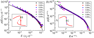
Figure 14: Scaling collapse for the two cases: (a) $\delta=0.30$ (tuned spinodal criticality) and (b) $\delta=0.46$ (BD criticality). Insets show schematic stress-strain curves around spinodal $S$ and critical $C$ points.

Finally we show the difference in the nature of the scaling collapse of pre-yield data shows for the critical and the spinodal points. In all near-critical regimes, the stress-resolved energy distribution is of the form $p(E;\sigma)\sim E^{-\tau}f(-E/E_{c}(\sigma))$ and to obtain the functions $f$ and $E_{c}$, we need to re-plot our data using the normalized variables $E^{\prime}=E/E_{c}$ and $p^{\prime}=p(E)E_{c}^{\tau}$. We find two distinct regimes where such data collapse could be achieved.

In the interval $0.3<\delta<0.4$, our Fig. 15(a) shows the validity of the scaling ansatz in the cutoff region with $E_{c}(\sigma)\sim(\sigma_{y}-\sigma)^{-1/v}.$ Here $\sigma_{y}$ is the yield stress at $\gamma_{y}$, and $v$ is a constant. This scaling suggests tuned criticality; indeed, the spinodal point is associated not only with a particular strain but also with particular stress Procaccia et al. (2017b); da Rocha and Truskinovsky (2020). We show in Fig. 15(a) that $1/v\approx 1.6$, which is different, for instance, from the value predicted in the theory of mean-field depinning where $1/v=2.0$ Dahmen et al. (2009), see Section XI for the relevance of this comment.

Figure 15: Critical scaling for: (a) $\delta=0.30$ (tuned spinodal criticality) and (b) $\delta=0.46$ (extended BD criticality). .

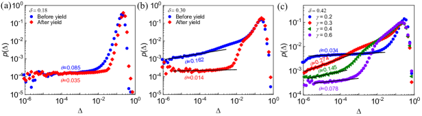
Figure 16: Distribution of stability measures $p(\Delta)$ at: (a) $\delta=0.18$ (weak disorder), (b) $\delta=0.30$ (intermediate disorder) and (c) $\delta=0.42$ (critical disorder). In (c) we effectively show the function of two variables $p(\Delta;\gamma)$.

The second region of scaling collapse is around $\delta\sim 0.42-0.46$. Here the cutoff follows the asymptotics $E_{c}(\sigma)\sim\exp(\sigma/\sigma_{0}),$ where $\sigma_{0}$ is a constant. The absence of stress tuning in this case can be explained by the fact that criticality in a strain-control ensemble makes stress poorly constrained, see Fig. 15(b). In other words, the BD critical point at $\delta\sim 0.42$ is localized in strain but not in stress.

VIII Excitation spectra

Recent advances in amorphous Lin et al. (2014) and crystal plasticity Ovaska et al. (2017) suggest that an important characterization of threshold-controlled dynamics comes from the density of elements with a given level of stability, also known as the excitation spectrum.

In our problem the natural stability measure is $\Delta=\bar{\xi}^{e}-\xi^{e}$ where $\xi^{e}=\xi-d(\xi)$ is the elastic strain and $\bar{\xi}^{e}=0.5$ is the stability threshold. The excitation spectrum is then the distribution $p(\Delta)$ of the local distances to a threshold above which a plastic correction takes place.

The form of the excitation spectrum in the limit $\Delta\to 0$ can be linked to the nature of intermittent fluctuations exhibited by the system Lin et al. (2015); Lin and Wyart (2016). Of particular interest is the “pseudogap” exponent $\theta(\gamma,\delta)$ entering the asymptotics $p(\Delta)\sim\Delta^{\theta}$ at $\Delta\to 0$ Karmakar et al. (2010); Müller and Wyart (2015).

We recall that in the case of classical depinning of an elastic manifold in random media, when yielding of a given site can only increase the load of other sites, it was shown that $\theta=0$ Fisher (1998). Another paradigmatic case is plasticity of amorphous glasses Lin et al. (2014); Shang et al. (2020b) where $\theta>0$ which was linked to the fact that the elastic long range interaction kernel is sign-indefinite.

While the depinning remains one of the main paradigms of plastic yielding in crystals Friedman et al. (2012); Ovaska et al. (2015), it was also realized stress transfer in crystal plasticity is sign-indefinite Bakó et al. (2007); Ispánovity et al. (2014); Lehtinen et al. (2016), and an extensive study Ovaska et al. (2017) produced a singular excitation spectrum with the exponent $\theta>0$ showing dependence on quenched disorder. The excitation spectra generated in our numerical experiments are summarized in Fig. 16.

When the quenched disorder is weak, see Fig. 16(a), the pre- and post-yield exponents $\theta$ agree. The obtained spectrum is almost gap-less with very small value of $\theta>0$. This is an indication of weak criticality Hentschel et al. (2015); Tyukodi et al. (2019); Ferrero and Jagla (2019b); Franz and Spigler (2017); Shang et al. (2020a) when the probability to find infinitesimal energy barrier is finite but close to zero. In such states the system is close to being elastic with dislocation microstructures characterized by high energy and low stability. Such systems are usually ’marginally stable’ in the sense that instabilities start to occur as soon as infinitesimal extra loading is applied, with glasses near and above jamming point as a prominent example Müller and Wyart (2015). Based only on the value of the exponent $\theta\sim 0$ it would be difficult to distinguish jamming from depinning in this case, however, since we know that $\tau\sim 1$ the jamming scenario should be clearly favored Ispánovity et al. (2014).

The excitation spectrum with $\theta\sim 0$ was also recorded in some mesoscopic models of amorphous plasticity Ferrero and Jagla (2019b); Tyukodi et al. (2019) and molecular dynamic simulations of glasses Shang et al. (2020b). As we have already mentioned in Section VII, this overall behavior is similar to the marginal response of mean-field systems described by the replica symmetry breaking framework and is also in agreement with what was found in simulations of three-dimensional systems of soft spheres, either at jamming or at slightly higher densities Franz and Spigler (2017).

At the intermediate level of disorder $\delta\sim 0.3$, see Fig. 16(b), we observe the emergence of a stronger pseudo-gap in pre-yield conditions, which we interpret as a signature of spinodal criticality. Instead, the post-yield regimes in this range of $\delta$ are characterized by $\theta\sim 0$. This may be explained by elastic depinning of an advancing surface separating a shear band from the rest of the crystal. Such surface would be generically produced by a spinodal SNAP event and its intermittent dynamics will be then controlled by sign-definite surface elasticity Pérez-Reche et al. (2008).

Around the BD critical point at $\delta\sim 0.42$ we observe a non-monotone dependence of the exponent $\theta$ on the loading parameter with a strong maximum around the yield strain $\gamma_{y}$, see Fig. 16(c). Before the yield, we obtain $\theta\sim 0$ which can be again interpreted as a signature of dislocation jamming. The yield at this level of disorder comes with an opening of a pseudo-gap indicating the development of the global connectivity of the energy landscape Müller and Wyart (2015); Zhang et al. (2017b). The increase of the applied strain $\gamma$ beyond the critical strain, decreases the pseudo-gap exponent again, bringing it to a plateau with $\theta\sim 0$, characterizing the stationary regime Ruscher and Rottler (2019). We can conjecture that this as a signature of the emerging depinning scaling. Indeed, in such regimes the self-induced inhomogenity, due to dislocation entanglements, can be expected to compromise the sign-indefinite nature of the elastic kernel with long range interactions progressively getting replaced by the largely ferromagnetic, short range interactions.

At even stronger quenched disorder ($\delta>0.6$ ) one can expect the loss of scaling and proliferation of uncorrelated POP events.

IX Mean field model

A simple mean field model can be used to rationalize at least some elements of the observed behavior in terms of macroscopic parameters. Suppose that the stress resolved evolution of the spatially averaged density of mobile dislocations $\rho$ is described by a stochastic kinetic equation Weiss et al. (2015)

$$\rho^{-1}d\rho/d\gamma=-c+\sqrt{2D}\eta(\gamma),$$ (20)

where the local shear strain $\gamma$ serves as a time-like parameter, $c\geq 0$ characterizes the rate of dislocation immobilization and the temperature-like parameter $D$ represents the intensity of the multiplicative mechanical noise with $\langle\eta(\gamma)\rangle=0$ and $\langle\eta(\gamma_{1}),\eta(\gamma_{2})\rangle=\delta(\gamma_{1}-\gamma_{2})$. Note that the lack of conventional dislocation sources in sub-micron crystals allows us to neglect here the Kocks-Mecking dislocation nucleation term Kocks and Mecking (2003); Weiss et al. (2015).

The stationary probability distribution in (20) is of a pure power law form $p_{s}(\rho)\sim\rho^{-\alpha}$ with the exponent $\alpha=1+c/D$. In the framework of our automaton we can interpret $\rho$ as the density of mobile dislocation during an avalanche at a given value of the loading $\gamma$. We can then write $\rho(\gamma)=n(\gamma)/N^{2}$, where $n(\gamma)$ is the number of dislocations moved during an avalanche. Our numerical experiments suggest that the avalanche energy $E$ is a disorder independent linear function of the total distance traveled by mobile dislocations during an avalanche $\bar{l}$, see Fig. 17(b), and that $\bar{l}\sim n$, see Fig. 17(c). Therefore $E\sim\rho$, see Fig. 17(a), and we can conclude that the exponent $\alpha$ in the mean field model is the same as the exponent $\tau$ in the automaton model. The relation $\alpha=\tau$, relying on the fact that for nano-crystals the mean free path is controlled only by the strength of quenched disorder (a proxy of the crystal size), is not applicable to bulk materials where one can expect that $\alpha=2\tau-1$ Weiss et al. (2015).

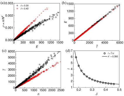
Figure 17: (a) Relation between the density of mobile dislocations $\rho$ and avalanche energy $E$ for representative disorders $\delta=0.30,0.42$; (b) dependence of $E$ on the total distance covered by dislocations during an avalanche $\bar{l}$; (c) dependence of $\bar{l}$ on the number of moving dislocations $n$; (d) Internal length scale $l$ as a function of disorder strength $\delta$.

For single slip pure nano-crystals with weak disorder dislocation immobilization can be neglected, so $c/D\ll 1$, and the stochastic evolution of $\rho$ governed by (20) reduces in this case to a geometric Brownian motion with $\alpha\sim 1$. In the automaton model we observe in the low-disorder limit dislocation self-organization, governed exclusively by elastic long-range elastic interactions Ispánovity et al. (2014); Weiss (2019), and recover the same value of the exponent $\tau\sim 1$. With increasing disorder, the immobilization rate $c$ should increase leading to a higher value of $\tau$, which is in qualitative agreement with our numerical experiments.

The crossover from $D$-dominated brittle regimes ($c<D$ with stochastic term in (20) controlling dynamics) to $c$-dominated ductile regimes ($c>D$ with deterministic term in (20) controlling dynamics) can be expected where the mechanical agitation is balanced by dislocation self-locking ($c\sim D$). Even though our oversimplified model (20) is not designed to capture the avalanche distribution in ductile regime, it is of interest to use our numerical results for reformulating the above limits in terms of crystal sizes.

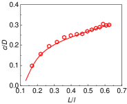
Figure 18: Dependence of the exponent $c/D$ in the post-yield regime on the dimensionless parameter $R=L/l$ for $h^{*}=0.395$ and $L=1$

Consider first the mean free path $l=\bar{l}/n$, characterizing dislocation glide before it gets immobilized. In Fig. 17(d) we show its dependence of disorder strength $\delta$ obtained from our numerical experiments. To obtain an analytical relation we can assume that only defects with the strength above some threshold $h^{*}$ participate in immobilization and that they form a regular lattice with spacing $l$. Then we can write

$$L/l\sim(1-\operatorname{erf}(h^{*}/(\sqrt{2}\delta)))^{1/2}.$$ (21)

Our Fig. 17(d) shows that this relation provides a perfect fit for the empirical curve if the stress threshold takes the value $h^{*}=0.395$. It also suggests that in the automaton model the mean free path of dislocations $l$, setting an intrinsic internal length scale, is indeed controlled by the tails of the disorder distribution.

Given that we know the relation $\tau(\delta)$ for post- yield regimes from our numerical experiments (see Fig. 12(a)), and using the relation $\alpha=\tau$, we can now obtain a relation between $c/D$ and $R=L/l$, see Fig. 18. It provides the desired quantitative description of the crossover from brittle (nano-crystalline) to (ductile) micro-crystalline plasticity.

Indeed, the effective temperature $D$ should depend only weakly on the system size $L$. It is defined instead by the locking strength of defects, which means that it increases with $l$. At the same time, it is clear that the rate of dislocation reactions (in particular our parameter $c$ controlling immobilization) increases with $L$ Zhang et al. (2017a). Therefore, in either very small and/or very weakly disordered samples $c<D$ and the response must be brittle. Conversely, in either bigger or more disordered samples one can expect to reach the ductile phase where $c>D$. This is what the curve shown in Fig. 18 implies.

X Cyclic loading

The mechanical response to monotone loading carries a memory of the initial state and in our tests, the preparation was entirely dislocation-free, as the goal was to simulate the plastic deformation of ultra-small systems (nano-particles and nano-pillars) Sharma et al. (2018b); Mordehai et al. (2018). To obtain the generic response, one can prime the crystal by subjecting it to cyclic protocol. If the strain amplitude of such pre-loading extends beyond the yield, a crystal becomes dislocations-rich already after a first cycle, independently of the initial disorder.

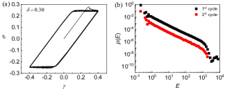
Figure 19: (a) Strain-stress curves for the crystals showing six loading-unloading cycles; (b) Avalanche distributions of cyclically loaded crystals during the first and the second cycles; the first cycle here is understood as a monotone loading path. Here: $\delta=0.30.$

The resulting self-induced disorder can be expected to quickly overtake the quenched disorder. As a result, the dimensionless parameter $R$ will increase due to the decrease of the dislocation mean free path $l$, which is now controlled by the density of the generated dislocations. This will lead to mild ductility ($R>1$) of even sub-micron crystals but without strain-hardening because of the remaining single-slip arrangement of plastic flow.

The typical stress-strain curves generated by the automaton model in quasi-static cyclic loading conditions are illustrated in Fig. 19(a). Brittleness indeed disappears already after the first load reversal even for the case of relatively weak initial disorder. The decrease in yield stress is consistent with the observations of softening in nano-crystals in response to the increase in the number of initial dislocations Bei et al. (2008a).

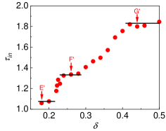
Figure 20: Disorder dependence of the integrated exponent $\tau_{int}$ in the case of cyclic loading.

In Fig. 19(b) we show how a typical avalanche distribution changes after the first cycle for $\delta=0.30$. One can see that the originally super-critical avalanche distribution, involving characteristic system size events, is replaced by a near-critical distribution that is basically maintained with subsequent cyclic loading. A robust range of scale-free behavior with a stable exponent $\tau$ emerges after shakedown. This observation suggests that a strongly ductile regime, with $R\gg 1$ and the manifest loss of scaling, cannot be achieved by cyclic loading at least at this strength of quenched disorder.

In Fig. 20 we show the disorder dependence of the stabilized cycle-integrated exponent $\tau_{in}$ which emerges in the case of sufficiently large amplitude of cyclic loading. The $\tau_{in}(\delta)$ curve shows distinctly three characteristic plateaux corresponding to the same three main scaling regimes which we identified in Section VII and can conditionally label as glassy, spinodal and critical. While the values of the exponents in Fig. 20 and in Fig. 12(a) do not match exactly due to the different nature of these exponents (stress-resolved vs. cycle-integrated) and different conditions (cyclic vs. monotone loading), the main trends appear to be well maintained.

Thus, at low strength of quenched disorder (plateau around point $E^{\prime}$) we obtain the value of the exponent reminiscent of the one in mean field spin-glasses and suggesting that dislocations can self-organize into a marginally stable (jammed) state. At the intermediate level of disorder (plateau around point $F^{\prime}$) we see the scaling which we previously associated with spinodal criticality when a SNAP even produces a system size effective manifold which evolves through classical elastic depinning. Finally, at sufficiently large strength of quenched disorder (plateau around point $G^{\prime}$), we observe a stretched scaling range associated with the critical BD transition.

In this analysis, we have identified two major crossover regimes. The first one, from $E^{\prime}$ to $F^{\prime}$, is similar to the jamming-to-depinning transition studied numerically by DDD approach in Ovaska et al. (2015). The second one, from $F^{\prime}$ to $G^{\prime}$, is similar to the spinodal-to-critical transition studied analytically at the mean field level in Ozawa et al. (2018); Popović et al. (2018); da Rocha and Truskinovsky (2020). While in previous work these crossovers were associated exclusively with changing disorder, here we interpret them as a feature of a size effect.

Finally, we note that our observation about the disappearance of brittleness in cyclic loading can potentially be used to turn fragile nano-crystals into mildly ductile nano-crystals Papanikolaou et al. (2017). Given the vulnerability of brittle ultra-small structures, the possibility to enhance ductility by purely mechanical means is of considerable interest for applications Zhang et al. (2017a). Moreover, by effectively increasing the strength of quenched disorder, such ’training’ can be expected to bring the crystal closer to the critical state Perez-Reche et al. (2016).

XI Compatible disorder

In addition to disorder, characterized by the random function $h_{i,j},$ and representing pre-stress acting directly on the longitudinal strain variable $\zeta_{i,j}$ and indirectly on the shear strain variable $\xi_{i,j}$, one can also introduce a disorder-related pre-stress $g_{i,j}$ acting directly on $\xi_{i,j}$ Tang et al. (2020). Then the energy density takes more symmetric form Salman and Truskinovsky (2011, 2012b):

$$f(\xi_{i,j},\zeta_{i,j})=\frac{K}{2}\zeta_{i,j}^{2}+\frac{1}{2}(\xi_{i,j}-d_{i,j}(\xi))^{2}-h_{i,j}\zeta_{i,j}-g_{i,j}\xi_{i,j}.$$ (22)

Note that in contrast to $h_{i,j},$ the disorder $g_{i,j}$ acts on the primary order parameter variable locally as in the conventional RFIM Nandi et al. (2016). Such ’local’ disorder can be viewed as resulting from lattice-compatible obstacles inhibiting or promoting plastic slip only in the narrow vicinity of a compact source of the disorder. One can think, for instance, about locked dislocation multi-poles, whose long-range fields are effectively screened. ’Local’ disorder may also be related to lattice-scale inhomogeneities lowering or raising the Peierls stress point-wise.

Suppose that both disorder fields, $h$ and $g$, are drawn independently in each lattice cell from Gaussian distributions

$$p_{s}(r)=(2\pi\delta_{s}^{2})^{-1/2}\exp{(-r^{2}/(2\delta_{s}^{2}))},$$ (23)

where $s=(g,h)$. In the previous Sections we used the special notation $\delta\equiv\delta_{h}$ but here, to distinguish the two, we’ll keep the notation $\delta_{h}$.

The specificity of the disorder $g_{i,j}$, representing essentially a residual plastic strain, is that it can be simply combined in the energy density with the actual plastic strain $d_{i,j}$. For instance, to account for $g$ in the Fourier representation of the elastic solution, it sufficient to replace the field $\hat{d}(\mathbb{q})$ by the sum $\hat{g}(\mathbb{q})+\hat{d}\mathbb{(}\mathbb{q})$. We can then write

$$\hat{\xi}(\mathbb{q})=\gamma\delta(\mathbb{q})+\hat{L}(\mathbb{q})\left[\hat{d}(\mathbb{q})+\hat{g}(\mathbb{q})\right]+\hat{L}_{h}(\mathbb{q})\hat{h}(\mathbb{q}),$$ (24)

where the kernels $\hat{L}_{h}(\mathbb{q})$ and $\hat{L}_{h}(\mathbb{q})$ were introduced in (8) and (16), respectively.

To perform a direct comparison of the two types of disorder we need to assess the action of the fields $g_{i,j}$ and $h_{i,j}$ on the same strain variable. A natural way to do this is to eliminate the linear non-order parameter $\zeta_{i,j}$ adiabatically and to evaluate the role of disorder $h_{i,j}$ in the ’condensed’ model containing only one variable $\xi_{i,j}$. The crucial observation is that the strain variables $\xi_{i,j}$ and $\zeta_{i,j}$ are not independent even though they are not coupled explicitly in the energy density. The implicit coupling can be revealed if we recall the constraint of geometric compatibility  Shenoy and Lookman (2008).

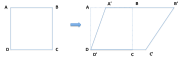
Figure 21: Generic deformation of a mesoscopic square element.

From now on, it will be convenient to deal directly with physical variables rather than their Fourier transforms. Since our displacement field is scalar, the generic deformation of an element is highly anisotropic, see Fig. 21. The geometrical meaning of the two strain variables $\xi_{i,j}$ and $\zeta_{i,j}$ becomes apparent from the identification: $D^{\prime}C^{\prime}=1+\zeta_{i,j}$, $A^{\prime}B^{\prime}=1+\zeta_{i,j+1}$, $AA^{\prime}=\xi_{i,j}$, and $BB^{\prime}-CC^{\prime}=\xi_{i+1,j}$, where $ABCD$ is the square lattice element before the deformation and $A^{\prime}B^{\prime}C^{\prime}D^{\prime}$ is its image after the deformation, see Fig. 21.

It is straightforward to see that $AA^{\prime}+A^{\prime}B^{\prime}=1+BB^{\prime},$ and since $D^{\prime}C^{\prime}-CC^{\prime}=1$ we obtain in terms of $\xi_{i,j}$ and $\zeta_{i,j}$ Perez-Reche et al. (2016)

$$\xi_{i,j}-\xi_{i+1,j}=\zeta_{i,j}-\zeta_{i,j+1}.$$ (25)

Eq. 25 is a discrete analog of the classical Saint-Venant compatibility relations in continuum linear elasticity, see Treibergs et al. (2020) for the general analysis. It provides a constraint on the variables $\xi_{i,j}$ and $\zeta_{i,j}$ which is inherently nonlocal. If we now complement the condition (25) with our (single) mechanical equilibrium condition (4), we obtain a closed system representing in our case the classical Beltrami-Michell equations of classical elasticity Kucher et al. (2004).

To simplify notations we’ll be using lexicographic order of the elements expressing the Cartesian coordinates $(i,j)$ in terms of a single label $p=i+(j-1)N$ that takes values $p=1,2,\dots N\times N$. With these notations, a second-order tensor can be represented as a vector and a fourth-order tensor takes the form of as a matrix.

Consider for simplicity an externally unloaded body. Using the lexicographic notations we can write the equilibrium equation $\partial\Phi/\partial u=0$, in the form $K\zeta=h+{\bf A}(\xi-(d+g)),$ where ${\bf A}$ is a standard forth order tensor with constant entries. Substituting the expression for $\zeta$ into the compatibility equations (25) we obtain $h+{\bf A}(\xi-(d+g))=K{\bf B}\xi,$ where ${\bf B}$ is another standard forth order tensor; the explicit expressions for the tensors ${\bf A}$ and ${\bf B}$ can be found in Perez-Reche et al. (2016).

Using the obtained relations we can write the explicit representation of elastic solution in the form

$$\xi=({\bf I}-K{\bf A}^{-1}{\bf B})^{-1}\left[(d+g)-{\bf A}^{-1}h\right]=0.$$ (26)

We stress that the ’local’ disorder $g$ enters (26) as a quenched analog of a compatible plastic deformation. Instead the incompatible disorder $h$ enters the solution nonlocally in the sense that a residual stress $h$ placed in the element $\{k,l\}$ affects the actual elastic strain field $\xi$ in every other element $\{i,j\}$.

Note also that since plastic slip develops to minimize elastic energy, it effectively acts to bring the expression in square brackets in (26) closer to zero. It can then compensate a compact source of the disorder $g$ by yielding locally, at the location of such source. Instead, a compact source of the disorder $h$ can be compensated only by a broadly distributed plastic slip. To illustrate this point, we compare in Fig. 22 the responses of a loaded crystal with either ’nonlocal’ disorder $h$ or ’local’ disorder $g$ present in the form of a point source.

Specifically, we consider the disorder fields $g_{i,j}=p\delta_{i,0}\delta_{j,0}$ and $h_{i,j}=q\delta_{i,0}\delta_{j,0}$, where $\delta_{i,j}$ is the Kronecker delta, and choose the amplitudes $p=q$ to ensure that when only one of these fields is present at $\gamma=0$ no plasticity occurs. Then, in each of these two cases, we find the smallest increment $\delta\gamma$ initiating a slip in at least one element.

If $p=0$ and $q=0.5$ (minimal ’nonlocal’ disorder), the avalanche resulting from such loading is dramatic with many dislocations forming collectively and the system developing a macroscopic shear band with complex internal structure, see Fig. 22(a). If $p=0.5$ and $q=0$ (minimal ’local’ disorder), two dislocations of opposite sign nucleate at the source of the disorder and move apart to finally annihilate at the boundaries where we impose periodic boundary conditions. Therefore the response remains contained and reduces to the formation of a microscopic slip at the scale of a single element, see Fig. 22(b).

The observed nonlocal (global) accommodation of the disorder $h$ is possible only when the system is sufficiently homogeneous. In the presence of a substantial ’local’ disorder $g$, the ability of the system to generate such global response may be compromised. At sufficient strength of ’local’ disorder $\delta_{g}$ the coherent accommodation of ’nonlocal’ disorder $\delta_{h}$ will become impossible, and as we argue below, this can change the avalanche scaling in a fundamental way.

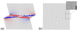
Figure 22: Comparison of the displacement fields resulting from pointwise ’nonlocal’ and ’local’ disorders: (a) $g_{i,j}\equiv 0$ and $h_{i,j}=0.5\delta_{i,0}\delta_{j,0}$; (b) $g_{i,j}=0.5\delta_{i,0}\delta_{j,0}$ and $h_{i,j}\equiv 0$. The ’nonlocal’ disorder produces a shear band with many dislocations. The ’local’ disorder produces a single slip due to nucleation and subsequent annihilation of a pair of dislocations. Here $K=2$, $N=256$; colors reflect the level of longitudinal strain.

To avoid any dependence on the initial preparation of the sample, we have chosen to present the interplay between the two types of disorder, ’local’ and ’nonlocal’ in the setting of cyclic loading. Our numerical experiments, summarized in Fig. 23(a), show that when a weak ’local’ disorder $\delta_{g}=0.3$ is combined with a weak ’nonlocal’ disorder $\delta_{h}=0.3$, the overall mechanical response is ductile. The initial softening behavior, observed in crystals with $\delta_{g}=0$, is replaced by the more conventional hardening behavior. At large strains the stress response shows a robust yielding plateau independently of the configuration of disorder. The overall response is reminiscent of the classical strain-hardening behavior exhibited by bulk FCC and BCC materials Suresh (1998).

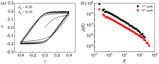
Figure 23: (a) Strain-stress curves for the crystals subjected to six loading unloading cycles; (b) Avalanche distributions of cyclically loaded crystals for the first and the second cycles; the first cycle is understood as the monotone loading path. Here $\delta_{h}=\delta=0.30$, $\delta_{g}=0.30$.

From Fig. 23(b) we see that even a weak ’local’ disorder is sufficient to suppress super-criticality and to completely eliminate system-size events. This observation agrees with the idea that such disorder generates local inhomogeneities which inhibit global response. However, the increase of the cut-off size in the second cycle suggests that a correlated behavior, reminiscent of disorder-induced self-organization towards classical criticality in RFIM model Dahmen and Sethna (1996); da Rocha and Truskinovsky (2020), can still take place.

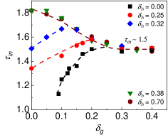
Figure 24: Effect of the ’local’ disorder $\delta_{g}$ on the (integrated) scaling exponent $\tau_{in}$ for the case of cyclic loading.

In Fig. 24 we show how the different configurations of ’local’ and ’nonlocal’ disorder strengths affect the cycle-averaged (integrated) scaling exponents $\tau_{in}$. When the ’local’ disorder is weak, we recover the after-yield behavior studied in Section X. At stronger ’local’ disorder, the dependence of the exponent $\tau_{in}$ on the ’nonlocal’ disorder progressively diminishes. Beyond $\delta_{g}\sim 0.25$ it completely disappears, and the exponent stabilizes around the value $\tau_{in}\sim 3/2$. Given that the statistics is mostly acquired during hardening-free yield, see Fig. 23, one can expect the stress-resolved value of the exponent $\tau$ to be similar to the aggregate value $\tau_{in}$ Durin and Zapperi (2006). In this case the obtained exponent value suggests mean field criticality Dahmen and Sethna (1996); da Rocha and Truskinovsky (2020). In other words, the abundance of ’local’ disorder apparently trivializes the scaling picture, erasing the non-universality and promoting a universal response of the athermally driven infinite dimensional RFIM dominating the response of amorphous solids Ozawa et al. (2018, 2020); Bhaumik et al. (2019); Franz and Rocchi (2020).

XII Conclusions

To address the fundamental question why the dislocation avalanches in sub-micron crystals of both face-centered cubic (fcc) and body-centered cubic (bcc) metals exhibit ’wild’ scaling, while the associated bulk crystals are ’mild’, we conducted a range of numerical experiments using a minimal integer-automaton model of crystal plasticity.

Our approach to the study of the size effect is based on the assumption that the dominance of surface-induced dislocation activity in sub-micron crystals can be modeled by the scarcity of conventional bulk dislocation sources. To justify this assumption, we compared the effects of extreme miniaturization in our physical experiments on Mo micro-pillars with the behavior of the numerical model as we progressively diminished the strength of quenched disorder. In both cases, we observed the same second-order BD transition, which provides the basic explanation for the ultimate shift from ’wildness’ to ’mildness’ in the fluctuational response with non-universality ultimately emerging as a size-effect.

The detailed transition from largely brittle to mostly ductile behavior was conceptualized as a complex three-stage crossover. The individual transitions are from spin-glass-type marginality, characteristic of very small, almost disorder free crystals, through spinodal/depinning criticality at intermediate sizes (moderate disorder level), to the classical BD criticality in larger, highly disordered crystals. In general, this scenario shows some similarity with the one observed in amorphous plasticity Ozawa et al. (2018); Popović et al. (2018), however, the nuanced picture in crystal plasticity appears to be more intricate.

In addition to monotone loading, we also considered large amplitude oscillatory shear loading protocols. We observed that brittleness disappears after cyclic loading, which suggests that nominally brittle sub-micron crystals can be ’trained’ to become ductile. However, the basic crossover structure, including the presence of three distinct universality classes, was shown not to be affected by the type of loading.

The non-universality of the scaling behavior progressively weakens as we complement the generic incompatible disorder, interacting with plasticity nonlocally, by the more special compatible disorder, which affects the plastic slip locally as, for instance, in RFIM model. Our numerical experiments suggest that the increase in the strength of the ’local’ disorder eventually restores universality bringing the system into the mean field type criticality class characteristic of amorphous solids.

Our schematic scalar model would have to be extended to the full tensorial theory based on nonlinear elasticity to obtain a more detailed description of crystal plasticity. This extension will allow one to distinguish between different crystallographic classes and different configurations of dislocation cores. Such a model should be able to reproduce dislocation walls and generate cell structures with realistic size distribution. A 3D theory of this type can also capture dislocation cross-slip and address hardening behavior. To study surface effects directly, one would need to come up with the boundary conditions allowing for dislocation nucleation on the surface. A path in this general direction has been recently sketched in Baggio et al. (2019).

XIII Acknowledgments

We thank N. Gorbushin, M. Mungan, F. Perez Reche and D. Vandembroucq for helpful discussions and Jin-yu Zhang for the characterization of dislocation structure. This work was supported by French-Chinese ANR-NSFC grant (ANR-19-CE08-0010-01 and 51761135031). P.Z. acknowledges additional support from China Scholarship Council and China Postdoctoral Science Foundation (grant 2019M653595).

References

- Han et al. (2015) W.-Z. Han, L. Huang, S. Ogata, H. Kimizuka, Z.-C. Yang, C. Weinberger, Q.-J. Li, B.-Y. Liu, X.-X. Zhang, J. Li, E. Ma, and Z.-W. Shan, Adv. Mater. 27, 3385 (2015).
- Maaß et al. (2012) R. Maaß, L. Meza, B. Gan, S. Tin, and J. R. Greer, Small 8, 1869 (2012).
- Mordehai et al. (2011) D. Mordehai, S.-W. Lee, B. Backes, D. J. Srolovitz, W. D. Nix, and E. Rabkin, Acta Mater. 13, 5202 (2011).
- Papanikolaou et al. (2017) S. Papanikolaou, Y. Cui, and N. Ghoniem, Modell. Simul. Mater. Sci. Eng. 26, 013001 (2017).
- Maaß and Derlet (2018) R. Maaß and P. M. Derlet, Acta Mater. 143, 338 (2018).
- Uchic et al. (2004) M. D. Uchic, D. M. Dimiduk, J. N. Florando, and W. D. Nix, Science 305, 986 (2004).
- Greer et al. (2005) J. R. Greer, W. C. Oliver, and W. D. Nix, Acta Mater. 53, 1821 (2005).
- Dimiduk et al. (2006) D. M. Dimiduk, C. Woodward, R. Lesar, and M. D. Uchic, Science 312, 1188 (2006).
- Zaiser (2006) M. Zaiser, Adv. Phys. 55, 185 (2006).
- Uchic et al. (2009) M. D. Uchic, P. A. Shade, and D. M. Dimiduk, Annu. Rev. Mater. Res. 39, 361 (2009).
- Csikor et al. (2007) F. F. Csikor, C. Motz, D. Weygand, M. Zaiser, and S. Zapperi, Science 318, 251 (2007).
- Friedman et al. (2012) N. Friedman, A. T. Jennings, G. Tsekenis, J.-Y. Kim, M. Tao, J. T. Uhl, J. R. Greer, and K. A. Dahmen, Phys. Rev. Lett. 109, 095507 (2012).
- Maass et al. (2015) R. Maass, M. Wraith, J. T. Uhl, J. R. Greer, and K. A. Dahmen, Phys. Rev. E Stat. Nonlin. Soft Matter Phys. 91, 042403 (2015).
- Ng and Ngan (2008) K. S. Ng and A. H. W. Ngan, Acta Mater. 56, 1712 (2008).
- Brinckmann et al. (2008) S. Brinckmann, J.-Y. Kim, and J. R. Greer, Phys. Rev. Lett. 100, 155502 (2008).
- Zaiser et al. (2008a) M. Zaiser, J. Schwerdtfeger, A. Schneider, C. Frick, B. G. Clark, P. Gruber, and E. Arzt, Philos. Mag. 88, 3861 (2008a).
- Papanikolaou et al. (2012) S. Papanikolaou, D. M. Dimiduk, W. Choi, J. P. Sethna, M. D. Uchic, C. F. Woodward, and S. Zapperi, Nature 490, 517 (2012).
- Zhang et al. (2017a) P. Zhang, O. U. Salman, J.-Y. Zhang, G. Liu, J. Weiss, L. Truskinovsky, and J. Sun, Acta Mater. 128, 351 (2017a).
- Cui et al. (2017) Y. Cui, G. Po, and N. Ghoniem, Phys. Rev. B 95, 064103 (2017).
- Wang et al. (2012) Z.-J. Wang, Z.-W. Shan, J. Li, J. Sun, and E. Ma, Acta Mater. 60, 1368 (2012).
- Chrobak et al. (2011a) D. Chrobak, N. Tymiak, A. Beaber, O. Ugurlu, W. W. Gerberich, and R. Nowak, Nature nanotechnology 6, 480 (2011a).
- Bei et al. (2008a) H. Bei, S. Shim, G. M. Pharr, and E. P. George, Acta Materialia 56, 4762 (2008a).
- Broberg (1999) K. B. Broberg, Cracks and fracture (Elsevier, 1999).
- Sharma et al. (2018a) A. Sharma, J. Hickman, N. Gazit, E. Rabkin, and Y. Mishin, Nat. Commun. 9, 4102 (2018a).
- Mordehai et al. (2018) D. Mordehai, O. David, and R. Kositski, Adv. Mater. 30, 1706710 (2018).
- Argon (2013) A. S. Argon, Philos. Mag. 93, 3795 (2013).
- Benzerga (2009) A. A. Benzerga, J. Mech. Phys. Solids 57, 1459 (2009).
- Motz et al. (2009) C. Motz, D. Weygand, J. Senger, and P. Gumbsch, Acta Mater. 57, 1744 (2009).
- Weiss et al. (2015) J. Weiss, W. B. Rhouma, T. Richeton, S. Dechanel, F. Louchet, and L. Truskinovsky, Phys. Rev. Lett. 114, 105504 (2015).
- Niiyama and Shimokawa (2015) T. Niiyama and T. Shimokawa, Phys. Rev. E Stat. Nonlin. Soft Matter Phys. 91, 022401 (2015).
- Miguel et al. (2001) M. C. Miguel, A. Vespignani, S. Zapperi, J. Weiss, and J. R. Grasso, Nature 410, 667 (2001).
- Ispánovity et al. (2014) P. D. Ispánovity, L. Laurson, M. Zaiser, I. Groma, S. Zapperi, and M. J. Alava, Phys. Rev. Lett. 112, 235501 (2014).
- Ovaska et al. (2015) M. Ovaska, L. Laurson, and M. J. Alava, Sci. Rep. 5, 10580 (2015).
- Chan et al. (2010) P. Y. Chan, G. Tsekenis, J. Dantzig, K. A. Dahmen, and N. Goldenfeld, Phys. Rev. Lett. 105, 015502 (2010).
- Zaiser and Nikitas (2007) M. Zaiser and N. Nikitas, J. Stat. Mech. 2007, P04013 (2007).
- Salman and Truskinovsky (2011) O. U. Salman and L. Truskinovsky, Phys. Rev. Lett. 106, 175503 (2011).
- Sparks and Maaß (2018) G. Sparks and R. Maaß, Phys. Rev. Materials 2, 120601 (2018).
- Song et al. (2019) H. Song, D. Dimiduk, and S. Papanikolaou, Phys. Rev. Lett. 122, 178001 (2019).
- Salman and Truskinovsky (2012a) O. U. Salman and L. Truskinovsky, Int. J. Eng. Sci. 59, 219 (2012a).
- Dahmen and Sethna (1996) K. Dahmen and J. P. Sethna, Phys. Rev. B Condens. Matter 53, 14872 (1996).
- Ozawa et al. (2018) M. Ozawa, L. Berthier, G. Biroli, A. Rosso, and G. Tarjus, Proc. Natl. Acad. Sci. U. S. A. 115, 6656 (2018).
- Procaccia et al. (2017a) I. Procaccia, C. Rainone, and M. Singh, Phys Rev E 96, 032907 (2017a).
- Popović et al. (2018) M. Popović, T. W. J. de Geus, and M. Wyart, Phys. Rev. E 98, 040901 (2018).
- Shang et al. (2020a) B. Shang, P. Guan, and J.-L. Barrat, Proc. Natl. Acad. Sci. U. S. A. 117, 86 (2020a).
- Maaß et al. (2013) R. Maaß, P. M. Derlet, and J. R. Greer, Scr. Mater. 69, 586 (2013).
- Sornette and Ouillon (2012) D. Sornette and G. Ouillon, Eur. Phys. J. Spec. Top. 205, 1 (2012).
- da Rocha and Truskinovsky (2020) H. B. da Rocha and L. Truskinovsky, Phys. Rev. Lett. 124, 015501 (2020).
- Zaiser et al. (2008b) M. Zaiser, J. Schwerdtfeger, A. S. Schneider, C. P. Frick, B. G. Clark, P. A. Gruber, and E. Arzt, Philos. Mag. 88, 3861 (2008b).
- Cui et al. (2020a) Y. Cui, G. Po, P. Srivastava, K. Jiang, V. Gupta, and N. Ghoniem, Int. J. Plast. 124, 117 (2020a).
- Sparks et al. (2019) G. Sparks, Y. Cui, G. Po, Q. Rizzardi, J. Marian, and R. Maaß, Phys. Rev. Materials 3, 080601 (2019).
- Chrobak et al. (2011b) D. Chrobak, N. Tymiak, A. Beaber, O. Ugurlu, W. W. Gerberich, and R. Nowak, Nat. Nanotechnol. 6, 480 (2011b).
- Lu et al. (2011) Y. Lu, J. Song, J. Y. Huang, and J. Lou, Nano Research 4, 1261 (2011).
- Bei et al. (2008b) H. Bei, S. Shim, G. M. Pharr, and E. P. George, Acta Mater. 56, 4762 (2008b).
- Issa et al. (2015) I. Issa, J. Amodeo, J. Réthoré, L. Joly-Pottuz, C. Esnouf, J. Morthomas, M. Perez, J. Chevalier, and K. Masenelli-Varlot, Acta Mater. 86, 295 (2015).
- Greer and Nix (2006) J. R. Greer and W. D. Nix, Phys. Rev. B Condens. Matter 73, 245410 (2006).
- Puglisi and Truskinovsky (2005) G. Puglisi and L. Truskinovsky, J. Mech. Phys. Solids 53, 655 (2005).
- Picard et al. (2004) G. Picard, A. Ajdari, F. Lequeux, and L. Bocquet, Eur. Phys. J. E Soft Matter 15, 371 (2004).
- Tyukodi et al. (2016) B. Tyukodi, S. Patinet, S. Roux, and D. Vandembroucq, Phys Rev E 93, 063005 (2016).
- Weiss (2019) J. Weiss, Philos. Trans. A Math. Phys. Eng. Sci. 377, 20180260 (2019).
- Deschamps et al. (2012) A. Deschamps, G. Fribourg, Y. Brechet, J. L. Chemin, and C. Hutchinson, Acta Mater. 60, 1905 (2012).
- Maloney and Lemaître (2006) C. E. Maloney and A. Lemaître, Phys. Rev. E Stat. Nonlin. Soft Matter Phys. 74, 016118 (2006).
- Paladin and Vulpiani (1987) G. Paladin and A. Vulpiani, Phys. Rep. 156, 147 (1987).
- Mandelbrot (1989) B. B. Mandelbrot, in Fractals in geophysics (Springer, 1989) pp. 5–42.
- Meneveau and Sreenivasan (1991) C. Meneveau and K. Sreenivasan, J. Fluid Mech. 224, 429 (1991).
- Lopes and Betrouni (2009) R. Lopes and N. Betrouni, Med. Image Anal. 13, 634 (2009).
- Weiss (2001) J. Weiss, Eng. Fract. Mech. 68, 1975 (2001).
- Lebyodkin and Lebedkina (2006) M. A. Lebyodkin and T. A. Lebedkina, Phys. Rev. E Stat. Nonlin. Soft Matter Phys. 73, 036114 (2006).
- Salerno and Robbins (2013) K. M. Salerno and M. O. Robbins, Phys. Rev. E Stat. Nonlin. Soft Matter Phys. 88, 062206 (2013).
- Gimbert et al. (2013) F. Gimbert, D. Amitrano, and J. Weiss, EPL 104, 46001 (2013).
- Clauset et al. (2009) A. Clauset, C. R. Shalizi, and M. E. Newman, SIAM review 51, 661 (2009).
- Lehtinen et al. (2016) A. Lehtinen, G. Costantini, M. J. Alava, S. Zapperi, and L. Laurson, Phys. Rev. B Condens. Matter 94, 064101 (2016).
- Pázmándi et al. (1999) F. Pázmándi, G. Zaránd, and G. T. Zimányi, Phys. Rev. Lett. 83, 1034 (1999).
- Franz and Spigler (2017) S. Franz and S. Spigler, Phys Rev E 95, 022139 (2017).
- Berthier et al. (2019) L. Berthier, G. Biroli, P. Charbonneau, E. I. Corwin, S. Franz, and F. Zamponi, J. Chem. Phys. 151, 010901 (2019).
- Müller and Wyart (2015) M. Müller and M. Wyart, Annual Review of Condensed Matter Physics 6, 177 (2015).
- Pérez-Reche et al. (2008) F.-J. Pérez-Reche, L. Truskinovsky, and G. Zanzotto, Phys. Rev. Lett. 101, 27 (2008).
- Tyukodi et al. (2019) B. Tyukodi, D. Vandembroucq, and C. E. Maloney, Phys Rev E 100, 043003 (2019).
- Ferrero and Jagla (2019a) E. E. Ferrero and E. A. Jagla, Soft Matter 15, 9041 (2019a).
- Cui et al. (2020b) Y. Cui, G. Po, P. Srivastava, K. Jiang, V. Gupta, and N. Ghoniem, Int. J. Plast. 124, 117 (2020b).
- Zhang et al. (2016) X. Zhang, X.-C. Zhang, Q. Li, and F.-L. Shang, Chin. Physics Lett. 33, 106401 (2016).
- Ruscher and Rottler (2019) C. Ruscher and J. Rottler, arXiv preprint arXiv:1908.01081 (2019).
- Ferguson et al. (1999) C. D. Ferguson, W. Klein, and J. B. Rundle, Phys. Rev. E Stat. Phys. Plasmas Fluids Relat. Interdiscip. Topics 60, 1359 (1999).
- Nandi et al. (2016) S. K. Nandi, G. Biroli, and G. Tarjus, Phys. Rev. Lett. 116, 145701 (2016).
- Lin et al. (2014) J. Lin, E. Lerner, A. Rosso, and M. Wyart, Proc. Natl. Acad. Sci. U. S. A. 111, 14382 (2014).
- Liu et al. (2016) C. Liu, E. E. Ferrero, F. Puosi, J.-L. Barrat, and K. Martens, Phys. Rev. Lett. 116, 065501 (2016).
- Budrikis et al. (2017) Z. Budrikis, D. F. Castellanos, S. Sandfeld, M. Zaiser, and S. Zapperi, Nat. Commun. 8, 15928 (2017).
- Vojta (2006) T. Vojta, J. Phys. A Math. Gen. 39, R143 (2006).
- Procaccia et al. (2017b) I. Procaccia, C. Rainone, and M. Singh, Phys. Rev. E 96, 032907 (2017b).
- Dahmen et al. (2009) K. A. Dahmen, Y. Ben-Zion, and J. T. Uhl, Phys. Rev. Lett. 102, 175501 (2009).
- Ovaska et al. (2017) M. Ovaska, A. Lehtinen, M. J. Alava, L. Laurson, and S. Zapperi, Phys. Rev. Lett. 119, 265501 (2017).
- Lin et al. (2015) J. Lin, T. Gueudré, A. Rosso, and M. Wyart, Phys. Rev. Lett. (2015).
- Lin and Wyart (2016) J. Lin and M. Wyart, Phys. Rev. X 6, 011005 (2016).
- Karmakar et al. (2010) S. Karmakar, E. Lerner, and I. Procaccia, Phys. Rev. E Stat. Nonlin. Soft Matter Phys. 82, 055103 (2010).
- Fisher (1998) D. S. Fisher, Phys. Rep. 301, 113 (1998).
- Shang et al. (2020b) B. Shang, P. Guan, and J.-L. Barrat, Proc. Natl. Acad. Sci. U. S. A. 117, 86 (2020b).
- Bakó et al. (2007) B. Bakó, I. Groma, G. Györgyi, and G. T. Zimányi, Phys. Rev. Lett. 98, 075701 (2007).
- Hentschel et al. (2015) H. G. E. Hentschel, P. K. Jaiswal, I. Procaccia, and S. Sastry, Phys. Rev. E Stat. Nonlin. Soft Matter Phys. 92, 062302 (2015).
- Ferrero and Jagla (2019b) E. E. Ferrero and E. A. Jagla, Soft Matter 15, 9041 (2019b).
- Zhang et al. (2017b) D. Zhang, K. A. Dahmen, and M. Ostoja-Starzewski, Phys Rev E 95, 032902 (2017b).
- Kocks and Mecking (2003) U. F. Kocks and H. Mecking, Prog. Mater Sci. 48, 171 (2003).
- Sharma et al. (2018b) A. Sharma, J. Hickman, N. Gazit, E. Rabkin, and Y. Mishin, Nat. Commun. 9, 4102 (2018b).
- Perez-Reche et al. (2016) F. J. Perez-Reche, C. Triguero, G. Zanzotto, and L. Truskinovsky, Phys. Rev. B Condens. Matter 94, 144102 (2016).
- Tang et al. (2020) A. Tang, H. Liu, G. Liu, Y. Zhong, L. Wang, Q. Lu, J. Wang, and Y. Shen, Phys. Rev. Lett. 124, 155501 (2020).
- Salman and Truskinovsky (2012b) O. U. Salman and L. Truskinovsky, Int. J. Eng. Sci. 59, 219 (2012b).
- Shenoy and Lookman (2008) S. Shenoy and T. Lookman, Phys. Rev. B Condens. Matter 78, 144103 (2008).
- Treibergs et al. (2020) A. Treibergs, A. Cherkaev, and P. Krtolica, Int. J. Solids Struct. 184, 248 (2020).
- Kucher et al. (2004) V. Kucher, X. Markenscoff, and M. Paukshto, J. Elast. 74, 135 (2004).
- Suresh (1998) S. Suresh, Fatigue of Materials (Cambridge University Press, 1998).
- Durin and Zapperi (2006) G. Durin and S. Zapperi, J. Stat. Mech. 2006, P01002 (2006).
- Ozawa et al. (2020) M. Ozawa, L. Berthier, G. Biroli, and G. Tarjus, Phys. Rev. Research 2, 023203 (2020).
- Bhaumik et al. (2019) H. Bhaumik, G. Foffi, and S. Sastry, arXiv preprint arXiv:1911.12957 (2019).
- Franz and Rocchi (2020) S. Franz and J. Rocchi, J. Phys. A: Math. Theor. (2020).
- Baggio et al. (2019) R. Baggio, E. Arbib, P. Biscari, S. Conti, L. Truskinovsky, G. Zanzotto, and O. U. Salman, Phys. Rev. Lett. 123, 205501 (2019).