Event reconstruction for KM3NeT/ORCA using convolutional neural networks

Abstract

The KM3NeT research infrastructure is currently under construction at two locations in the Mediterranean Sea. The KM3NeT/ORCA water-Cherenkov neutrino detector off the French coast will instrument several megatons of seawater with photosensors. Its main objective is the determination of the neutrino mass ordering. This work aims at demonstrating the general applicability of deep convolutional neural networks to neutrino telescopes, using simulated datasets for the KM3NeT/ORCA detector as an example. To this end, the networks are employed to achieve reconstruction and classification tasks that constitute an alternative to the analysis pipeline presented for KM3NeT/ORCA in the KM3NeT Letter of Intent. They are used to infer event reconstruction estimates for the energy, the direction, and the interaction point of incident neutrinos. The spatial distribution of Cherenkov light generated by charged particles induced in neutrino interactions is classified as shower- or track-like, and the main background processes associated with the detection of atmospheric neutrinos are recognized. Performance comparisons to machine-learning classification and maximum-likelihood reconstruction algorithms previously developed for KM3NeT/ORCA are provided. It is shown that this application of deep convolutional neural networks to simulated datasets for a large-volume neutrino telescope yields competitive reconstruction results and performance improvements with respect to classical approaches.

1 Introduction

Precision measurements of the fundamental properties of neutrinos are one of the opportunities that might allow us to discover and understand the physics that exists beyond the established Standard Model of particle physics.

The detection of neutrinos, both for fundamental particle physics and high-energy astrophysics, can be achieved with the deep-sea and photon-detection technology that has been developed by the ANTARES [1] and KM3NeT [2] Collaborations for very-large-volume water-Cherenkov detectors.

KM3NeT/ORCA, the low-energy detector of KM3NeT, addresses the determination of a still unknown, but fundamental parameter of neutrino physics: the neutrino mass ordering. The experiment focuses on the measurement of the energy- and zenith-angle-dependent oscillation patterns of cosmic-ray-induced neutrinos with a few-GeV energy that originate in the atmosphere and traverse the Earth [3].

The power to distinguish between the two different mass orderings is linked to the detection of an excess or deficit of neutrino events in different regions of these oscillation patterns. This sensitivity increases with better energy and zenith-angle resolution and flavour identification for the interacting neutrinos, and finer control of systematic effects that influence the measurement. Therefore, one of the most important goals in the analysis of KM3NeT/ORCA data is the development and characterisation of neutrino event reconstruction and classification algorithms that improve these resolutions.

The neutrino detection principle of water- or ice-based large-scale Cherenkov detectors relies on the detection of Cherenkov photons induced by charged secondary particles created in a neutrino interaction with the target material. All neutrino flavours can interact through the weak neutral current (NC) mediated by the exchange of a $\text{Z}^{0}$ boson. This interaction results in a particle shower composed mainly of hadrons, generically referred to as a hadronic system, while the scattered neutrino escapes undetected. An interaction via the weak charged current (CC), with the exchange of a $\text{W}^{+}$ or $\text{W}^{-}$ boson, also often results in a hadronic shower at the interaction vertex. Additionally, a lepton of the same flavour as the interacting neutrino is created, which carries a fraction of the incoming neutrino energy.

A muon neutrino or muon antineutrino CC interaction, $\mathchoice{\vbox{\offinterlineskip\halign{\hfill#\hfill\cr\vbox{\hrule width=3.99994pt}\cr\vskip-1.29167pt\cr\hbox to10.00002pt{$\mathchar 300\relax\hfil\mathchar 301\relax$}\cr\vskip-1.29167pt\cr$\displaystyle\upnu$\cr}}}{\vbox{\offinterlineskip\halign{\hfill#\hfill\cr\vbox{\hrule width=3.99994pt}\cr\vskip-1.29167pt\cr\hbox to10.00002pt{$\mathchar 300\relax\hfil\mathchar 301\relax$}\cr\vskip-1.29167pt\cr$\textstyle\upnu$\cr}}}{\vbox{\offinterlineskip\halign{\hfill#\hfill\cr\vbox{\hrule width=2.5pt}\cr\vskip-1.29167pt\cr\hbox to8.00003pt{$\mathchar 300\relax\hfil\mathchar 301\relax$}\cr\vskip-1.29167pt\cr$\scriptstyle\upnu$\cr}}}{\vbox{\offinterlineskip\halign{\hfill#\hfill\cr\vbox{\hrule width=1.99997pt}\cr\vskip-1.29167pt\cr\hbox to6.99997pt{$\mathchar 300\relax\hfil\mathchar 301\relax$}\cr\vskip-1.29167pt\cr$\scriptscriptstyle\upnu$\cr}}}\kern-1.72218pt^{\;{}\text{CC}}$, results in an outgoing muon in the final state. From now on the term ‘neutrino’ refers always to both neutrinos and antineutrinos, if not stated otherwise. The muon appears as a track-like light source in the detector, and can therefore be identified with good confidence, depending on its track length. The visible trajectory of the muon is determined by its energy loss, and in water it amounts to about roughly 4 m per GeV of muon energy for the relevant energy regime of a few GeV.

At the energy ranges considered in KM3NeT/ORCA, all neutrino-nucleon NC, ${}_{\text{e}}^{\text{CC}}$, and ${}^{\text{CC}}$ interactions, with the exception of roughly 18 % of tau leptons decaying into muons, create a particle shower of a few meters length, that appears as an elongated, but localised, light source compared to the typical distance scales between the detector elements ($920\text{\,}\mathrm{m}$, cf. Sec. 2.1). This event type is referred to as shower-like. The outgoing electron from a ${}_{\text{e}}^{\text{CC}}$ event initiates an electromagnetic shower, a cascade of $\text{e}^{\pm}$-pairs, while the hadronic system, typically at the neutrino interaction vertex, develops into a hadronic shower with large event-to-event fluctuations and a possibly complex structure of hadronic or electromagnetic sub-showers, depending on the decay modes of individual particles in the shower.

Although an electromagnetic shower consists of many $\text{e}^{\pm}$-pairs with rather short path lengths (about 36 cm radiation length in water, see Sec. 33.4.2. in Ref. [4]) and overlapping Cherenkov cones, the small pair opening angle preserves the Cherenkov angle peak of the total angular light distribution. This results in a single Cherenkov ring projected onto the plane perpendicular to the shower axis. Similarly, each hadronic shower particle with energy above the Cherenkov threshold will produce a Cherenkov ring. Therefore, hadronic showers show a variety of different signatures due to the various possible combinations of initial hadron types, their momenta and the diversity of their hadronic interactions in the shower evolution.

While electromagnetic cascades show only negligible fluctuations in the number of emitted Cherenkov photons and in the angular light distribution, hadronic cascades show significant intrinsic fluctuations in the relevant few-GeV energy range. These intrinsic fluctuations of hadronic cascades and the resulting limitations for the energy and angular resolutions have been studied in detail in Ref. [5].

Dedicated reconstruction algorithms for track-like and shower-like events have been developed for KM3NeT/ORCA based on maximum-likelihood methods. Additionally, a machine-learning algorithm, based on Random Forests [6], has been employed successfully to classify track-like, shower-like, and background events. These algorithms, their implementation and performance are described in the KM3NeT Letter of Intent [2].

In the last few years, significant progress has been made in the machine-learning community due to the advent of deep-learning techniques. A particularly successful deep-learning concept is that of a deep neural network. Specialised neural network model architectures have been designed for individual use cases. In the field of computer vision, Convolutional Neural Networks (CNNs) have led to a strong increase in image recognition performance. From 2010 to 2016, the error rates in e.g. the popular ImageNet image classification challenge improved by a factor of 10 [7][8].

Since the data of many high-energy physics experiments can be interpreted in a way similar to typical images in the computer vision domain, these techniques have already been exploited by several experiments [12, 11, 10, 9]. As an example, the classification performance of neutrino interactions in the NOvA experiment has been significantly improved by employing CNNs compared to classical reconstruction tools [13].

In this paper, we present for the first time the application of CNNs to detailed Monte Carlo simulations of a large water-Cherenkov neutrino detector with the goal to provide a comprehensive reconstruction pipeline for KM3NeT/ORCA, starting from data at the level of the data-acquisition system. For this purpose, a Keras-based [14] software framework, called OrcaNet [15], has been developed that simplifies the usage of neural networks for neutrino telescopes. Here, we apply this framework to neutrino event reconstruction and classification in KM3NeT/ORCA, and compare the results achieved with the algorithms described in Ref. [2]. We note that also these algorithms continue to be developed and improved in KM3NeT.

The paper is organised as follows. Section 2 introduces the KM3NeT/ORCA detector, the Monte Carlo simulation chain used to generate training and validation data for the CNNs and introduces relevant aspects of the trigger algorithms. Section 3 gives a brief introduction to the main functional features of the employed CNNs, while Section 4 details the developed pre-processing chain that creates suitable input images from the Monte Carlo simulation data. Section 5 provides an overview of the general network architecture that is shared by all CNNs that have been designed for the reconstruction and classification tasks, which together define the analysis pipeline for KM3NeT/ORCA. The concepts and performance of these specific CNNs, as well as exemplary comparisons to their counterpart algorithms, are explained in the next sections. Section 6 explains the background classifier, Section 7 the event topology classifier used to distinguish track-like and shower-like events, while Section 8 introduces event regression and its respective uncertainties, i.e. the reconstruction of the direction, energy, and vertex of the incident neutrinos. Section 9 summarises and concludes the paper.

2 The KM3NeT/ORCA experiment

The KM3NeT research infrastructure is under construction at two sites in the Mediterranean Sea. The KM3NeT/ORCA detector is located about $40\text{\,}\mathrm{km}$ off-shore of Toulon in the south of France. Its main goal is to detect atmospheric neutrinos with GeV energies ($340\text{\,}\mathrm{GeV}$), while KM3NeT/ARCA, located south-east of Sicily, aims to investigate astrophysical neutrinos. The main design principles and scientific goals of the experiment can be found in the KM3NeT Letter of Intent [2].

2.1 Layout of the detector

The detector volume of KM3NeT/ORCA will be instrumented with 115 Detection Units (DUs), which are vertical, string-like structures anchored to the seabed and held upright by a buoy at the top of the DU. Currently, the first six DUs have been installed and are operational. Each DU holds 18 Digital Optical Modules (DOMs). The DOMs contain 31 photomultiplier tubes (PMTs) with a diameter of 3" each. The PMTs are used to measure two quantities, the arrival time and the time range that the anode output signal remains above a tunable threshold (time-over-threshold, ToT) with a time resolution on the nanosecond scale. The ToT can be used as a proxy for the amount of light registered by the PMT. The vertical spacing between the DOMs on a single DU is on average $9\text{\,}\mathrm{m}$, while the average horizontal distance between the DUs is about $20\text{\,}\mathrm{m}$. This results in a total instrumented volume of about six megatons of seawater.

There are two main sources of background in KM3NeT/ORCA, namely atmospheric muons reaching the detector from above and random optical background due to beta decays of ${{}^{\text{40}}}\text{K}$ in seawater and bioluminescence. Optical background, which is dominated by decays of ${{}^{\text{40}}}\text{K}$, accounts for about $7\text{\,}\mathrm{kHz}$ of uncorrelated single photon noise per PMT with a rate of two-fold coincidences of about $500\text{\,}\mathrm{Hz}$ per DOM [16].

The atmospheric muon background can be reduced significantly by requiring the reconstructed vertex position to be inside or close to the instrumented detector volume. In addition, predominantly atmospheric muons enter the detector from above and therefore the atmospheric muon background can be further reduced by discarding events for which the direction of the emerging particle trajectory is reconstructed as downwards.

2.2 Monte Carlo simulations and trigger algorithms

Detailed Monte Carlo (MC) simulations of the detector response have been produced for three distinct types of triggered data, namely atmospheric muons, random noise and neutrinos. A detailed introduction to the KM3NeT simulation package and the trigger algorithms can be found in Ref. [2].

For neutrinos, ${}_{\text{e}}^{\text{CC}}$ and ${}^{\text{CC}}$ interactions on nucleons and nuclei in seawater have been simulated, while all NC interactions are represented by ${}_{\text{e}}^{\text{NC}}$, since the detector signature is identical for all flavours. Charged-current interactions of are neglected for simplicity, as the resulting detector signatures for the different decay modes of the tau lepton are very similar to either ${}_{\text{e}}^{\text{CC}}$ or ${}^{\text{CC}}$.

The distance between DUs for the simulations employed in this work is on average $23\text{\,}\mathrm{m}$ and hence $3\text{\,}\mathrm{m}$ larger than for the simulations used in Ref. [2]. The vertical inter-DOM spacing is set to $9\text{\,}\mathrm{m}$ on average, which was identified as optimal for the determination of the neutrino mass ordering in Ref. [2]. The highest level of simulated data consists of a list of hits, i.e.  time stamp, ToT, and identifier, for all PMTs in the detector. In addition to the signal hits induced by the interactions of neutrinos and by atmospheric muons in the sensitive detector volume, simulated background hits due to random noise are added such that the simulated triggered data matches the real conditions as closely as possible.

After hits have been simulated, several trigger algorithms that rely on causality conditions are applied. Once a trigger has fired to define an event, all hits that have fired the trigger, including signal and background hits, are labelled as triggered hits. Since the trigger algorithm is not fully efficient in identifying all signal hits, a larger time window than the one defined for the triggered hits is saved for further analysis. Assuming a triggered event with $t_{\text{first}}$ as the time of the first triggered hit and $t_{\text{last}}$ as the time of the last triggered hit, all photon hits in each PMT in a time window [$t_{\text{first}}-t_{\text{marg}}$, $t_{\text{last}}+t_{\text{marg}}$] are recorded, where $t_{\text{marg}}$ is defined by the maximum amount of time that a photon propagating in water would need to traverse the whole detector. As a result, the total time window of triggered neutrino events in KM3NeT/ORCA is about $3\text{\,}\mathrm{\SIUnitSymbolMicro s}$.

A summary with detailed information about the simulated data for KM3NeT/ORCA is shown in Tab. 1.

Event type	$\text{E}_{\text{gen}}$ spectrum	$\text{N}_{\text{trig}}$ [10${}^{\text{6}}$]	Energy range
Atmospheric muon	-	65.2	-
Random noise	-	23.3	-
${}_{\text{e}}^{\text{NC}}$	$\text{E}^{\text{-1}}$	1.1	$15\text{\,}\mathrm{GeV}$
${}_{\text{e}}^{\text{NC}}$	$\text{E}^{\text{-3}}$	3.7	$3100\text{\,}\mathrm{GeV}$
${}_{\text{e}}^{\text{CC}}$	$\text{E}^{\text{-1}}$	1.5	$15\text{\,}\mathrm{GeV}$
${}_{\text{e}}^{\text{CC}}$	$\text{E}^{\text{-3}}$	4.4	$3100\text{\,}\mathrm{GeV}$
${}^{\text{CC}}$	$\text{E}^{\text{-1}}$	1.7	$15\text{\,}\mathrm{GeV}$
${}^{\text{CC}}$	$\text{E}^{\text{-3}}$	8.3	$3100\text{\,}\mathrm{GeV}$

Table 1: List of Monte Carlo simulations for a KM3NeT/ORCA detector composed of 115 DUs. The first column reports the simulated event type. The neutrino simulations comprise neutrino and antineutrino interactions of the indicated type. The second column specifies the power law used to simulate the energy spectrum of the interacting neutrinos. A reweighting scheme is used in this work, where appropriate, to simulate an atmospheric neutrino flux model [17]. $\text{N}_{\text{trig}}$ is the number of events that remain after triggering. Atmospheric muons have been simulated with the MUPAGE package [18]. Random noise events have been simulated conservatively with a $10\text{\,}\mathrm{kHz}$ single rate per PMT with additional n-fold coincidences ($600\text{\,}\mathrm{Hz}$ two-fold, $60\text{\,}\mathrm{Hz}$ three-fold, $7\text{\,}\mathrm{Hz}$ four-fold, $0.8\text{\,}\mathrm{Hz}$ five-fold and $0.08\text{\,}\mathrm{Hz}$ six-fold [16]). Time-varying increases of the hit rate due to bioluminescence in seawater have not been simulated.

3 Convolutional neural networks

This section introduces the concepts and nomenclature used in the description of the networks that have been developed and used in this work.

Convolutional neural networks [20, 19] form a specialised class of deep neural networks. Generally, neural networks are used in order to approximate a function $f(x)$, which maps a certain number of inputs $x_{i}\in X$ to some outputs $y_{i}\in Y$. The goal is then to find an approximation $\hat{f}(x)$ to the function $f(x)$ that describes the relationship between the inputs $x_{i}$ and the outputs $y_{i}$. Neural networks are based on the concept of artificial neurons that are arranged in layers. For a fully connected neural network, each neuron in a layer is connected to all neurons in the previous layer.

Stacking multiple layers of neurons can be interpreted as multiple functions that are acting on the input $X$ in a chain. For a two-layer network and thus two functions $f^{(1)}$ and $f^{(2)}$ (the  $\hat{}$  symbol of $\hat{f}$ is neglected from this point on) this is:

$$f(x)=f^{(2)}(f^{(1)}(x)).$$ (3.1)

Here, $f^{(1)}$ refers to the first layer in the network and $f^{(2)}$ to the second. The first layer of a neural network is called the input layer, the intermediate layers are called the hidden layers and the last layer is called the output layer.

In order to learn the relationship between $(X,Y)$, learnable weights are used for each neuron. If a single neuron has inputs $x_{i}$, then each $x_{i}$ has a weight $w_{i}$ associated to this input. Additionally, a single, learnable bias parameter is added in order to increase the flexibility of the model to fit the data. This process in a neuron, consisting of the weights $w_{i}$ and the bias $b$, shows a linear response:

$$f_{\Sigma}=\sum_{i=1}^{n}w_{i}x_{i}+b.$$ (3.2)

However, many physical processes in nature are inherently nonlinear. To account for this, the output of the transfer function can be wrapped in another, nonlinear function. Additionally, it can be shown that a nonlinear, two-layer neural network can approximate any function (Chap. 6.4.1. in Ref. [20]). The most commonly used, nonlinear function is the rectified linear unit (ReLU):

$$f_{\text{ReLU}}(x)=\max(0,x).$$ (3.3)

Such functions are called activation functions or layers.

The weights of each neuron get updated iteratively during a training process. For this purpose, one needs to define a so-called cost or loss function, which measures the distance between the output of the neural network $f(x)=y_{\text{reco}}$ and the ground truth $y_{\text{true}}$. This can for example be done by measuring the mean squared error and minimising $(y_{\text{true}}-y_{\text{reco}})^{2}$.

Typically, iterative gradient descent (Chap. 4.3. in Ref. [20]) based optimisation algorithms are used that minimise the cost function until a low value is achieved. During this training process, the cost error is back-propagated using a back-propagation algorithm (Chap. 6.5. in Ref. [20]), which allows for the tuning of the neural network’s weights.

Convolutional neural networks are frequently used in domains, where the input can be expected to be image-like, i.e. in image or video classification. Therefore, several changes are made in the architecture of CNNs compared to fully connected neural networks. The main concepts of convolutional neural networks are based on only locally and not fully connected networks and on parameter sharing between certain neurons in the network.

Typical input images to convolutional neural networks are two-dimensional (2D). However, since most images are coloured, they in fact are encoded by three dimensions (3D): width, height and channel. Here, the channel dimension specifies the brightness for each colour channel (red, green and blue) of the image. This three dimensional array is then used as input to the first convolutional layer.

Similar to the input layer, the neurons in a convolutional layer are also arranged in three dimensions, called width, height and depth. As already mentioned, one of the main differences between convolutional layers and fully connected layers is that the neurons inside a convolutional layer are only connected to a local region of the input volume. This is often called the receptive field of the neuron. The connections of this local area to the neuron are local in space (width, height), but they are always full along the depth of the input volume. Hence, for a $\text{[32}\times\text{32}\times\text{3]}$ image (width, height, channel) and receptive field size of 5 pixels, each neuron in the first convolutional layer is connected to a local $\text{[5}\times\text{5}\times\text{3]}$ (width, height, depth) patch of the input. To each of these connections, a weight is assigned, such that each neuron has a [$\text{5}\times\text{5}\times\text{3}$] weight matrix, which is often called the kernel or filter. These weights are used in performing a dot product between the receptive field of the neuron and its associated kernel, also called the convolution process. Here, the total number of parameters for the single neuron would be $\text{5}\cdot\text{5}\cdot\text{3}+\text{1}~{}(\text{bias})=\text{76}$. Additionally, each neuron at the same depth level covers a different part of the image with its receptive field. For more information the reader is referred to Refs. [20, 19].

For CNNs, an important assumption is that abstract image structures, such as edges, occur multiple times in the image. Under this assumption, the neurons at a certain depth can share their weights, which significantly reduces the number of parameters in the network. The number of parameters in CNNs can be further reduced with the aid of pooling layers, which reduce the dimensionality of the layer outputs by selecting or combining the neuron outputs [20, 19].

For the training of a neural network, the data are split up into a training, validation, and test dataset. The network is trained on the training dataset and validated by applying the network to the validation dataset. Once the training is finished, the network is applied to the test dataset to determine its performance. If the value of the loss function is significantly greater for the training dataset than for the validation dataset, this is called overfitting with respect to the training dataset. The smaller the size of the training dataset, the higher the probability that the network will focus on the peculiarities of individual input images instead of generalising generic image features. In order to avoid overfitting, so-called regularisation techniques such as dropout layers have been developed [21]. In a dropout layer, inputs are randomly set to zero with a probability defined by the dropout rate $\delta$. In order to set up a basic convolutional neural network, the convolutional layers are stacked. After the last convolutional layer, the multi-dimensional output array is reshaped without ordering into a one-dimensional array by a flattening layer. A small fully-connected network can then be added, in order to connect the outputs of the last convolutional layer to the output neurons of the full network.

4 Data pre-processing

For each hit in a simulated event, the PMT identifier, i.e. the relative coordinate of the hit PMT in a DOM, is recorded. Additionally, the time at which the PMT signal crosses the discriminator threshold, and the measured ToT, are stored. However, the ToT value itself is not used as input for the CNNs. In order to feed this four-dimensional event data to a CNN, the hits can be binned into rectangular pixels, such that each image encodes three spatial dimensions (XYZ) and the time dimension T.

4.1 Spatial binning

The number of pixels required to resolve the spatial coordinates of the individual PMTs inside the DOMs would be very large, and most bins would be empty due to the sparsely instrumented detector volume. Therefore, the pixelation is defined such that exactly one DOM fits into one bin, while some bins remain empty due to the detector geometry. In the case of the full KM3NeT/ORCA detector, this results in a $\text{11}\times\text{13}\times\text{18}$ (XYZ) pixel grid. The information regarding which PMT in a DOM has been hit is discarded. This is corrected for by adding a PMT identifier dimension to the pixel grid, resulting in a XYZP grid. Since one DOM holds 31 PMTs, the final spatial shape of such an image is $\text{11}\times\text{13}\times\text{18}\times\text{31}$ (XYZP). Such image types can also be found in classical computer vision tasks, e.g. as coloured videos. The only difference is that in a conventional video the Z-coordinate is replaced by the time and the PMT identifier is replaced by the red-green-blue colour information.

4.2 Temporal Binning

The indispensable piece of information still missing in these images is the time at which a hit has been recorded. This information can be added as an additional dimension, such that the final image of an event is five-dimensional: XYZTP.

The time resolution in KM3NeT/ORCA is of the order of nanoseconds [22]. As explained in section 2.2, the time length of an event is about $3\text{\,}\mathrm{\SIUnitSymbolMicro s}$, implying 3000 bins for the time dimension to reach nanosecond resolution. However, with each additional bin, the size of the event image gets larger and this leads to additional computations in the first layer of a CNN. Hence, the number of bins of the final image should be as low as possible, while still containing the relevant timing information.

Most hits that lie outside the time range of the triggered hits are background hits and not signal hits. Therefore, background hits can be discriminated against to some extent by selecting the time range in which most signal hits are found. Investigating the distribution of the time of the signal hits relative to the mean of the triggered hit times in individual events, as depicted in Fig. 1 for ${}^{\text{CC}}$ events, shows that it is asymmetric and that the relevant time range can be reduced significantly for the image generation binning.

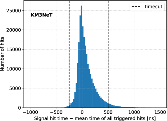
Figure 1: Time distribution of ${}^{\text{CC}}$ signal hits relative to the mean time of the triggered hits calculated for each individual event. For this distribution, about 3000 ${}^{\text{CC}}$ events in the energy range from $3\text{\,}\mathrm{GeV}100\text{\,}\mathrm{GeV}$ have been used, cf. Tab. 1. The dashed line in black indicates a possible timecut for the time range used to generate the CNN input images.

Since the time range covered by the triggered hits is different for each event, the time range selection is defined relative to the mean time of the triggered hits for each event. As can be seen in Fig. 1, only a small fraction of the signal hits are removed, as indicated by the timecut defined by the dashed, black lines. A compromise needs to be found between the width of the timecut window and the number of time bins, implying a certain time resolution available to the network. The specific values of the timecuts used in this work are reported in the respective image generation sections of the presented CNNs. The timecut window is a parameter that can be further optimised with respect to the final performance of a trained neural network. In this work, no such parameter optimisation studies have been carried out for any of the presented CNNs, which implies that their performance for specific use cases can likely be improved further.

4.3 Multi-image Convolutional Neural Networks

After binning, the resulting images are five-dimensional: XYZTP. In order to train the neural networks presented in this paper, the deep learning framework TensorFlow [23] has been used in conjunction with the Keras [14] high-level neural network programming library. However, TensorFlow does not support convolutional layers which accept more than four dimensions as input, since five dimensional inputs are not a usual case in computer vision. Hence, the five dimensions of the XYZTP images need to be reduced to four dimensions, such that one can use three-dimensional convolutional layers. To this end, one image dimension is summed up, i.e. the information of individual PMTs in a DOM is discarded, such that the resulting image is only four-dimensional (XYZT). However, a second image of the same event is then fed to the network (XYZP) that recovers the information regarding which PMT in a DOM has been hit, but discards its hit time. Since these images only differ in the 4th dimension, i.e. the depth dimension of a convolutional layer, the images can be stacked in this dimension. For example, an XYZP image of dimension $\text{11}\times\text{13}\times\text{18}\times\text{31}$ can be combined with an XYZT image of dimension $\text{11}\times\text{13}\times\text{18}\times\text{N}_{\text{T}}$ into a single, stacked XYZ-T/P image of dimension $\text{11}\times\text{13}\times\text{18}\times(\text{N}_{\text{T}}+\text{31})$. These images lack the information about the hit time for a specific PMT, if more than one hit has occurred on a DOM in an event.

Significant gains in performance for all CNN applications in this work were observed when using this stacking method, as compared to just supplying a single XYZT image. Furthermore, it will be demonstrated that networks with such input limitations can still match or outperform the KM3NeT/ORCA reconstruction algorithms as presented in Ref. [2].

5 Main network architecture

Four-dimensional images that have been created from simulated events are fed as input to a CNN. All networks that have been designed for a specific task in this work share a common architecture. The CNNs consist of two main components: the convolutional part with the convolutional layers and a small fully-connected network in the end. The convolutional part consists of convolutional blocks, each of them containing a convolutional layer, a batch normalisation layer [24], an activation layer, and, optionally, a dropout [21] or a pooling layer. The batch normalisation layer usually enables a faster and more robust training process of deep neural networks by normalising, scaling and shifting the output of the convolutional layer. The scaling and shifting transform is controlled by learnable parameters during the training process. Recent studies indicate that the batch normalisation method smoothes the optimisation landscape and induces a more predictive and stable behaviour of the gradients, allowing for faster training [25].

In the three-dimensional convolutional layer, the weights are initialised based on a uniform distribution whose variance is calculated according to Ref. [26], while the biases are set to zero. Additionally, the kernel size is three ($\text{3}\times\text{3}\times\text{3}$), the stride, i.e. the step size in shifting the convolutional kernel, is one ($\text{1}\times\text{1}\times\text{1}$) and zero-padding (Chap. 9 in Ref. [20]) is used. For the batch normalisation layers, the standard parameters from Ref. [24] are used. After this, a ReLU activation layer is added. These three layers are found in all convolutional blocks that are used in this work. Additionally, optional maximum pooling and dropout layers are added. In the case of maximum pooling layers, zero-padding is not applied. A scheme of these convolutional blocks is shown in Tab. 2.

Layer type	Properties
Convolution	kernel size ($\text{3}\times\text{3}\times\text{3}$), uniform initialisation [26], zero-padding
Batch normalisation	parameters as in Ref. [24]
Activation	ReLU
Maximum pooling	optional, no zero-padding
Dropout	optional

Table 2: Scheme of a convolutional block used for all CNNs defined in this work.

Furthermore, all models use the Adam gradient descent optimiser [27] with standard parameter values, except for the parameter $\epsilon$, which is increased from its default value of $\text{10}^{\text{-8}}$ to $\text{10}^{\text{-1}}$. A larger value of $\epsilon$ results in smaller weight updates after each training step. In our case, it has been observed that the network occasionally did not start to learn, depending on the random initialisation of the parameters. This could be fixed by changing the value of $\epsilon$ to $\text{10}^{\text{-1}}$ as suggested in Ref. [28], while significant drawbacks, such as a slower training convergence due to smaller weight updates, have not been observed. The weights of the neural network are updated after one batch of images is passed through the network. This is known as batch gradient descent. The batch size is defined as the number of images contained in one batch. The batch size in the training for all presented CNNs is generally set to 64 and the learning rate, i.e. the step size in the Adam algorithm for the update of the weights is annealed exponentially.

The training of all presented networks has been executed at the TinyGPU cluster at the RRZE computing centre . It consists of 32 nodes with 4 GPUs each. The GPUs are either Nvidia GTX1080, GTX1080Ti, RTX2080 Ti, or Tesla V100. All CNNs in this work have been trained with CUDA 10 [29]. In order to train the networks, an open-source software framework called OrcaNet [15] has been developed, which is intended as a high-level application programming interface on top of Keras [14], specifically suited to the large datasets that frequently occur in astroparticle physics.

6 Background classifier

An essential part of the KM3NeT/ORCA reconstruction pipeline is the background classifier, which discriminates atmospheric muons and random noise from neutrino-induced events. For this purpose, the employed classification algorithm is based on a Random Forest (RF) [6] method. The inputs of the RF are high-level observables (features), mainly determined from likelihood-based track and shower reconstruction algorithms. In this section, an alternative classifier based on CNNs is presented and its performance is compared to the RF classifier.

6.1 Image generation

As outlined in Sec. 4.3, XYZ-T/P images are used as input to the network. For both event images, i.e. the XYZT and XYZP components of the stacked XYZ-T/P image, a timecut has been defined, as introduced in Sec. 4.2. The signal hit time distribution of atmospheric muons, relative to the mean time of all triggered hits, is shown in Fig. 2. This distribution has a larger variance than for neutrino events shown in Fig. 1. The reason is that, on average, atmospheric muons traverse larger parts of the detector compared to the secondary particles of the GeV-scale neutrino interactions of interest. Hence, the timecut window for all event classes has been set conservatively based on atmospheric muon events, resulting in a width of $950\text{\,}\mathrm{ns}$.

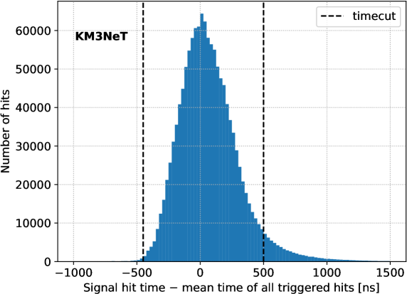
Figure 2: Time distribution of signal hits in atmospheric muon events relative to the mean time of the triggered hits calculated for each individual event. For this distribution, about 3000 atmospheric muon events have been used. The dashed black line indicates the timecut, set to an interval of [$-$450\text{\,}\mathrm{ns}$,+$500\text{\,}\mathrm{ns}$$], that has been applied for the generation of the background classifier images.

The timecut for this distribution, as indicated in Fig. 2, has been set to an interval of [$-$450\text{\,}\mathrm{ns}$,+$500\text{\,}\mathrm{ns}$$], keeping more early signal hits than late hits. The reason for this is that events which produce late hits are typically energetic and leave a longer trace in the detector. Hence, they can be better reconstructed than less energetic atmospheric muons that only produce a few hits at the edge of the detector. Consequently, cutting away a few late hits has a small effect compared to discarding early hits from a low-energy atmospheric muon event, which already produces a low number of hits.

The number of time bins is set to 100, such that the XYZT images have dimensions of $\text{11}\times\text{13}\times\text{18}\times\text{100}$. The resulting time resolution of each time bin is $9.5\text{\,}\mathrm{ns}$, which translates to about $2\text{\,}\mathrm{m}$ of photon propagation distance. Adding the information of the 31 PMTs per DOM, as described in Sec. 4.3, yields final event images that have a dimension of $\text{11}\times\text{13}\times\text{18}\times\text{131}$.

6.2 Network architecture

The CNN network architecture for the background classifier is based on the three-dimensional convolutional blocks introduced in Sec. 5, with two additional fully-connected layers, also called dense layers, at the end. The output layer of the CNN is composed of two neurons, such that the network only distinguishes between neutrino and non-neutrino events. An overview of the final network structure is shown in Tab. 3.

Building block / layer	Output dimension
XYZ-T Input	11 $\times$ 13 $\times$ 18	$\times$	100
XYZ-P Input	11 $\times$ 13 $\times$ 18	$\times$	31
Final stacked XYZ-T + XYZ-P Input	11 $\times$ 13 $\times$ 18	$\times$	131
Convolutional block 1 (64 filters)	11 $\times$ 13 $\times$ 18	$\times$	64
Convolutional block 2 (64 filters)	11 $\times$ 13 $\times$ 18	$\times$	64
Convolutional block 3 (64 filters)	11 $\times$ 13 $\times$ 18	$\times$	64
Convolutional block 4 (64 filters)	11 $\times$ 13 $\times$ 18	$\times$	64
Convolutional block 5 (64 filters)	11 $\times$ 13 $\times$ 18	$\times$	64
Convolutional block 6 (64 filters)	11 $\times$ 13 $\times$ 18	$\times$	64
Max pooling (2,2,2)	5 $\times$ 6 $\times$ 9	$\times$	64
Convolutional block 1 (128 filters)	5 $\times$ 6 $\times$ 9	$\times$	128
Convolutional block 2 (128 filters)	5 $\times$ 6 $\times$ 9	$\times$	128
Convolutional block 3 (128 filters)	5 $\times$ 6 $\times$ 9	$\times$	128
Convolutional block 4 (128 filters)	5 $\times$ 6 $\times$ 9	$\times$	128
Max pooling (2,2,2)	2 $\times$ 3 $\times$ 4	$\times$	128
Flatten	3072
Dense + ReLU	128
Dense + ReLU	32
Dense + Softmax	2

Table 3: Network structure of the background classifier’s three-dimensional CNN model with XYZ-T/P input. No dropout is used due to the large training dataset of $\text{42.6}\times\text{10}^{\text{6}}$ training events.

Initially, a CNN with three output neurons was tested, so that neutrinos, atmospheric muons and random noise events could be classified separately. However, it was observed that the three-class CNN performed slightly worse than the two-class CNN that distinguishes only neutrino events from all others. This is due to the fact that the network cannot prioritise neutrino versus non-neutrino classification in the three-class case. A mistakenly classified atmospheric muon, e.g., classified as a random noise event, has the same effect on the total loss as an atmospheric muon classified as a neutrino.

No regularisation techniques, such as dropout, are added to the network. The training dataset is large enough, cf. Sec. 6.3, so that virtually no overfitting occurs, i.e. the training-phase loss is of the same order as the loss during the validation phase.

6.3 Preparation of training, validation and test data

For the training of the background classifier, the simulated data from Tab. 1 is split into a training, validation and test dataset.

In order to balance the datasets with respect to their class frequency, one could split the data into 50% neutrino and 50% non-neutrino events (25% atmospheric muons + 25% random noise). Considering that the neutrino sample has the lowest number of events (about $\text{22.8}\times\text{10}^{\text{6}}$), one would have to remove a significant fraction of the $\text{23.3}\times\text{10}^{\text{6}}$ generated random noise events, and of the $\text{65.1}\times\text{10}^{\text{6}}$ atmospheric muon events for a class-balanced data splitting. On the other hand, based on the RF background classifier, it can be expected that the final accuracy of the classifier should be close to 99%. Therefore, a balanced splitting of the data into 50% for each class is not necessary, in order to avoid a local minimum during the training process. The following data splitting is used: 1/3 neutrino events, 1/3 random noise events and 1/3 atmospheric muon events, and hence the final class balance is 1/3 neutrino events and 2/3 non-neutrino events. Using this data splitting and considering the number of MC events summarised in Tab. 1, the size of the used training dataset is larger compared to a 50/50 split. The fractions of different neutrino flavours and interaction types is kept as indicated in Tab. 1.

This rebalanced dataset is then split into 75% training, 2.5% validation, and 22.5% test events, which is a trade-off between maximizing the training dataset and retaining sufficient statistics for performance evaluations. Additionally, the events that have been removed to balance the dataset (mostly atmospheric muons) are added to the test dataset. In total, the training data contains about $\text{42.6}\times\text{10}^{\text{6}}$ events.

Using a Nvidia Tesla V100 GPU, it takes about a week to fully train this CNN background classifier. The time needed for the training scales more weakly than linear with the number of time bins, which can be increased to improve the time resolution of the input images.

6.4 Performance and comparison to Random Forest classifier

The performance of the CNN background classifier is evaluated using the training and validation cross-entropy loss [20] of a specific classifier, the softmax classifier [20], as a function of the number of epochs, and is shown in Fig. 3. An epoch is defined as one training process of the CNN, using the entire training event dataset. The training is stopped after approximately two epochs, as the validation loss shows no further significant improvement. At the end of the training no overfitting is observed.

\begin{overpic}[width=292.69481pt,page=1]{img/bg_classifier/summary_plot.pdf} \put(40.0,66.0){{KM3NeT}} \end{overpic}

Figure 3: Training and validation cross-entropy loss of the background classifier during the training. Each data point of the training loss curve is averaged over 250 batches, i.e. $\text{250}\times\text{64}$ event images.

In order to compare the CNN performance to the RF background classifier, the same test dataset is used. A pre-selection of these events is carried out to reduce the fraction of atmospheric muon and random noise events to a few percent of all triggered events. For atmospheric muons this is achieved by selecting only events for which the reconstructed particle direction is below the horizon, i.e. which are up-going events in the detector. Furthermore, the events must have been reconstructed with high quality by the KM3NeT/ORCA maximum-likelihood reconstruction algorithms for either track-like or shower-like events. Finally, events reconstructed by the maximum-likelihood-based algorithms as originating from outside of the instrumented volume of the detector are removed.

In total, the pre-selected test dataset consists of about $\text{3.3}\times\text{10}^{\text{6}}$ neutrino, about $\text{6}\times\text{10}^{\text{4}}$ atmospheric muon and about $\text{4}\times\text{10}^{\text{4}}$ random noise events. This selection is used for all of the following performance evaluations.

In order to get a first impression of the CNN-based background classifier, the distribution of the neutrino class probability is investigated for all three event classes (neutrinos, atmospheric muons, random noise), cf. Fig. 4.

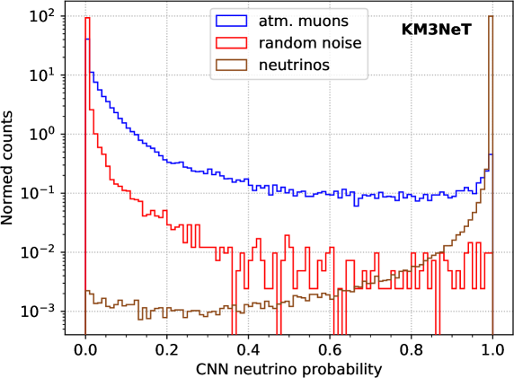
Figure 4: Distribution of the CNN neutrino probability for pre-selected atmospheric muon (blue), random noise (red), and neutrino (brown) events. All three distributions have been normalised to the area under each histogram.

Based on the results shown in Fig. 4, it can be seen that the rate of random noise events misclassified as neutrino-induced events is significantly lower than for atmospheric muons. Using the predicted probability for an event to be classified as neutrino-induced, a threshold value $p$ can be set to remove background events.

In order to quantify the performance of the CNN background classifier, the metric shown below is used to investigate the fraction of remaining atmospheric muon and random noise events for a given threshold value $p$. The atmospheric muon or random noise contamination, and the neutrino efficiency, are defined as:

$$\text{C}_{\upmu/\text{RN}}(p)=\frac{N_{\upmu/\text{RN}}(p)}{N_{\text{total}}(p)}\;,$$ (6.1)

$${}_{\text{eff}}(p)=\frac{N(p)}{N_{\upnu,\text{total}}}\;.$$ (6.2)

Here, $N_{\upmu/\text{RN}}$ is the number of atmospheric muon or random noise events, whose probability to be a neutrino-induced event is higher than $p$, while $N_{\text{total}}(p)$ accounts for the total number of events, after the same cut on $p$. Regarding the neutrino efficiency, $N(p)$ is the total number of neutrinos in the dataset whose neutrino probability is greater than the threshold value $p$, while $N_{\upnu,\text{total}}$ is the number of neutrinos in the dataset, without applying any threshold.

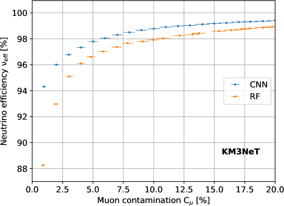
Figure 5: Neutrino efficiency, ${}_{\text{eff}}$, versus atmospheric muon event contamination, C, weighted with the Honda atmospheric neutrino flux [17] model. The CNN (RF) performance is depicted in blue (orange). All neutrinos from the pre-selected test dataset are included ($1\text{\,}\mathrm{GeV}100\text{\,}\mathrm{GeV}$).

Based on the results shown in Fig. 5 for the neutrino efficiency ${}_{\text{eff}}$ as a function of the residual atmospheric muon contamination C, it can be concluded that the CNN background classifier yields a higher neutrino efficiency, of the order of a few percent, for the same muon contamination compared to the RF background classifier.

Comparing different neutrino energy ranges, $1\text{\,}\mathrm{GeV}5\text{\,}\mathrm{GeV}$ in Fig. 6 and $10\text{\,}\mathrm{GeV}20\text{\,}\mathrm{GeV}$ in Fig. 7, it can be seen that the performance gap between the CNN and the RF classifier widens with increasing neutrino energy.

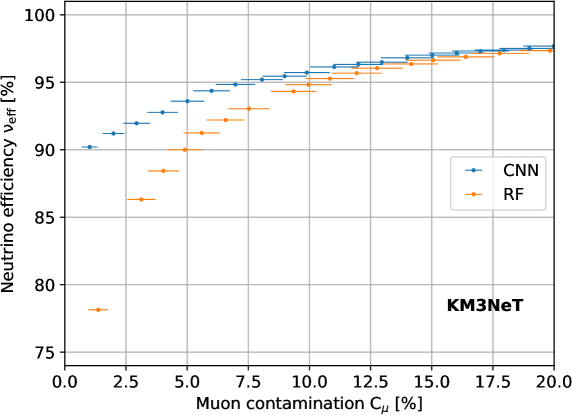
Figure 6: Neutrino efficiency, ${}_{\text{eff}}$, versus atmospheric muon event contamination, C, weighted with the Honda atmospheric neutrino flux [17] model. The CNN (RF) performance is depicted in blue (orange). Only neutrinos with a MC energy in the range of $1\text{\,}\mathrm{GeV}5\text{\,}\mathrm{GeV}$ have been used.

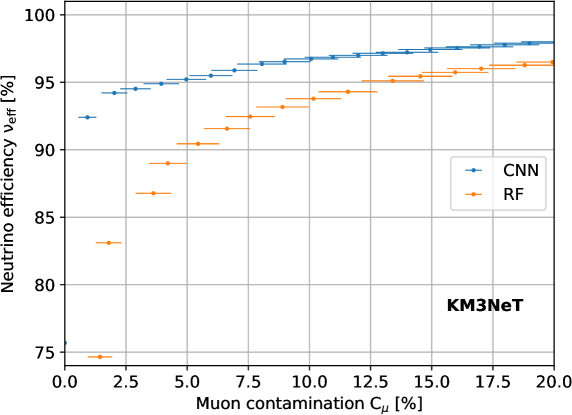
Figure 7: Neutrino efficiency, ${}_{\text{eff}}$, versus atmospheric muon event contamination, C, weighted with the Honda atmospheric neutrino flux [17] model. The CNN (RF) performance is depicted in blue (orange). Only neutrinos with a MC energy in the range of $10\text{\,}\mathrm{GeV}20\text{\,}\mathrm{GeV}$ have been used.

A possible explanation may be that small details in the distribution of the measured hits increase in importance if the neutrino events are less energetic and thus produce less hits. Then, the limitations of the input images, which do not contain the full information about an event, may become more relevant compared to events with higher energies and many signal hits.

For random noise events, the performance of the CNN and the RF classifier are comparable. In particular, both methods achieve about 99% neutrino efficiency at 1% random noise event contamination. As expected, the suppression of atmospheric muon events is significantly more difficult.

7 Event topology classifier

Similar to the background classifier, a RF is used in the current KM3NeT/ORCA analysis pipeline to separate track-like from shower-like neutrino events. This section introduces a CNN-based event topology classifier that distinguishes between these two event types.

7.1 Image generation

The input event images for the CNN-based track–shower classifier are similar to the ones of the background classifier introduced in Sec. 6.1, i.e. the input also consists of XYZ-T/P images. The timecut for the hit selection is tighter with respect to the background classifier. Since background events have already been rejected by the background classifier, the data presented to the track–shower classifier are mostly neutrino interactions which produce secondary particles that, on average, traverse smaller parts of the detector compared to atmospheric muon events. The event class that shows the broadest signal hit time distribution is the class of ${}^{\text{CC}}$ events due to the outgoing muon. Therefore, the timecut of the track–shower classifier is set based on these events. The time distribution of signal hits relative to the mean time of the triggered hits for ${}^{\text{CC}}$ events is shown in Fig. 1. Based on this distribution the timecut is set to an interval of [$-$250\text{\,}\mathrm{ns}$,+$500\text{\,}\mathrm{ns}$$], as indicated by the dashed, black lines in Fig. 1.

Since the timecut interval is smaller than the one used for the background classifier, less time bins (60) are used for the time dimension. This implies a reduction of the time resolution of about 30% with respect to the background classifier, i.e. $12.5\text{\,}\mathrm{ns}$ per time bin. The light emission profile of hadronic and electromagnetic showers in the GeV range has an extension of at most a few metres, see Fig. 70 in Ref. [2]. Since a muon of comparable energy induces the emission of Cherenkov radiation along a significantly greater path length, the reduced time binning still provides a sufficient resolution to distinguish a shower-like from a track-like event topology, while significantly speeding up the training of the CNN. Consequently, the XYZT images now have $\text{11}\times\text{13}\times\text{18}\times\text{60}$ pixels.

7.2 Network architecture

The network architecture, as depicted in Tab. 4, is the same as in Sec. 6.2, except for additional dropout layers. Since the size of the training dataset is significantly smaller than that for the background classifier, overfitting can be observed without any regularisation. Thus, dropout layers with a rate of $\delta=0.1$ are added in every convolutional block and also in between the last two fully connected layers.

Building block / layer	Output dimension
XYZ-T Input	11 $\times$ 13 $\times$ 18	$\times$	60
XYZ-P Input	11 $\times$ 13 $\times$ 18	$\times$	31
Final stacked XYZ-T + XYZ-P Input	11 $\times$ 13 $\times$ 18	$\times$	91
Convolutional block 1 (64 filters, $\delta=\text{0.1}$)	11 $\times$ 13 $\times$ 18	$\times$	64
Convolutional block 2 (64 filters, $\delta=\text{0.1}$)	11 $\times$ 13 $\times$ 18	$\times$	64
Convolutional block 3 (64 filters, $\delta=\text{0.1}$)	11 $\times$ 13 $\times$ 18	$\times$	64
Convolutional block 4 (64 filters, $\delta=\text{0.1}$)	11 $\times$ 13 $\times$ 18	$\times$	64
Convolutional block 5 (64 filters, $\delta=\text{0.1}$)	11 $\times$ 13 $\times$ 18	$\times$	64
Convolutional block 6 (64 filters, $\delta=\text{0.1}$)	11 $\times$ 13 $\times$ 18	$\times$	64
Max pooling (2,2,2)	5 $\times$ 6 $\times$ 9	$\times$	64
Convolutional block 1 (128 filters, $\delta=\text{0.1}$)	5 $\times$ 6 $\times$ 9	$\times$	128
Convolutional block 2 (128 filters, $\delta=\text{0.1}$)	5 $\times$ 6 $\times$ 9	$\times$	128
Convolutional block 3 (128 filters, $\delta=\text{0.1}$)	5 $\times$ 6 $\times$ 9	$\times$	128
Convolutional block 4 (128 filters, $\delta=\text{0.1}$)	5 $\times$ 6 $\times$ 9	$\times$	128
Max pooling (2,2,2)	2 $\times$ 3 $\times$ 4	$\times$	128
Flatten	3072
Dense + ReLU	128
Dropout ( $\delta=\text{0.1}$ )	128
Dense + ReLU	32
Dense + Softmax	2

Table 4: Network structure of the track–shower classifier three-dimensional CNN model with XYZ-T/P input. The symbol $\delta$ specifies the dropout rate used in the respective convolutional block, cf. Sec. 3.

7.3 Preparation of training, validation and test data

In order to train the CNN track–shower classifier, only simulated neutrino events are used. The total neutrino dataset is rebalanced such that 50% of the events are track-like (${}^{\text{CC}}$) and 50% are shower-like. The shower class consists of 50% ${}_{\text{e}}^{\text{CC}}$ and 50% ${}_{\text{e}}^{\text{NC}}$. Additionally, the dataset has been balanced in such a way that the ratio of track-like to shower-like events is always one, independent of neutrino energy.

The rebalanced dataset is then split into three datasets with 70% training, 6% validation, and 24% test events. In total, the training dataset contains about $\text{1.3}\times\text{10}^{\text{7}}$ events.

Using a Nvidia Tesla V100 GPU, it takes about one and a half weeks to fully train this CNN track–shower classifier.

7.4 Performance and comparison to Random Forest classifier

The evolution of the cross-entropy loss [20] during the training is shown in Fig. 8.

\begin{overpic}[width=292.69481pt,page=1]{img/ts_classifier/summary_plot.pdf} \put(40.0,66.0){{KM3NeT}} \end{overpic}

Figure 8: Training (grey lines) and validation (black circles) cross-entropy loss of the track–shower classifier during the training process. Each line element of the training loss represents an average over 250 batches, i.e. $\text{250}\times\text{64}$ event images.

Even though the validation cross-entropy loss is within the fluctuations of the training loss curve at the end of the training, some minor overfitting occurs. The reason is that during the application of the trained network on the validation dataset, no neurons are dropped by the dropout layers, contrary to the training phase. Therefore, the validation loss should be lower than the average training loss, if no overfitting is observed. This can be seen by investigating the training and validation loss curves in the earlier stages of the training process, e.g. between epoch 0 and 3. Here, the validation loss is typically found at the bottom of the training loss curve.

The binned probability distribution for all used neutrino events with energies in the range of $1\text{\,}\mathrm{GeV}40\text{\,}\mathrm{GeV}$ to be classified as track-like is shown in Fig. 9. This energy range has been chosen since the classification performance saturates at about $40\text{\,}\mathrm{GeV}$, as can be seen in Fig. 10 and further discussed below. The classified neutrino events have been selected according to the criteria described in Sec. 6.4.

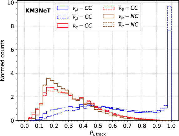
Figure 9: Distribution of the CNN track probability $P_{i,\text{track}}$ for pre-selected neutrino events of different flavours and interaction channels in the energy range of $1\text{\,}\mathrm{GeV}40\text{\,}\mathrm{GeV}$. All distributions have been normalised to the area under each histogram.

About 25% of ${}^{\text{CC}}$ and $\mkern 1.5mu\overline{\mkern-1.5mu\upnu\mkern-1.5mu}\mkern 1.5mu^{\text{CC}}$ events are identified as track-like events with a probability close to one. The correct identification of muon tracks increases with their length and hence with their energy. As the outgoing muon has on average higher energy for $\mkern 1.5mu\overline{\mkern-1.5mu\upnu\mkern-1.5mu}\mkern 1.5mu^{\text{CC}}$ than for ${}^{\text{CC}}$ events, $\mkern 1.5mu\overline{\mkern-1.5mu\upnu\mkern-1.5mu}\mkern 1.5mu^{\text{CC}}$ events have a higher probability to be identified as track-like.

The top panel of Fig. 10 shows the fraction of events classified as track-like as a function of the neutrino energy in the range of $1\text{\,}\mathrm{GeV}40\text{\,}\mathrm{GeV}$. An event is accepted if its CNN probability to be a track-like event is 0.5 or above. The fraction of correctly classified ${}^{\text{CC}}$ and $\mkern 1.5mu\overline{\mkern-1.5mu\upnu\mkern-1.5mu}\mkern 1.5mu^{\text{CC}}$ events rises strongly with neutrino energy. The reason is that the spatial and temporal distribution of hits induced by low-energy ${}^{\text{CC}}$ events is similar to that of shower-like events, since the outgoing muon stops at these energies after propagating only a few meters in the detector. Comparing ${}_{\text{e}}^{\text{CC}}$ and $\mkern 1.5mu\overline{\mkern-1.5mu\upnu\mkern-1.5mu}\mkern 1.5mu_{\text{e}}^{\text{CC}}$ with energies below $10\text{\,}\mathrm{GeV}$, it can be seen that $\mkern 1.5mu\overline{\mkern-1.5mu\upnu\mkern-1.5mu}\mkern 1.5mu_{\text{e}}^{\text{CC}}$ are more likely classified as track-like by the CNN classifier. This is again due to the fact that the outgoing charged lepton carries on average more energy in $\mkern 1.5mu\overline{\mkern-1.5mu\upnu\mkern-1.5mu}\mkern 1.5mu^{\text{CC}}$ interactions with respect to ${}^{\text{CC}}$ interactions. On the other hand, for energies below $10\text{\,}\mathrm{GeV}$, NC interactions have a lower misclassification rate compared to ${}_{\text{e}}^{\text{CC}}$ interactions, since there is no charged secondary lepton that could mimic the signature of a low-energy muon as induced in ${}^{\text{CC}}$ events. For energies above $10\text{\,}\mathrm{GeV}$ the opposite is true, since a localised and bright light source disfavours a ${}^{\text{CC}}$ event.

A measure for the separation power of the classifier is the difference between the fractions of recognised track-like events for ${}^{\text{CC}}$ ($\text{f}^{{}^{\text{CC}}}_{\text{track}}$, blue line) and ${}_{\text{e}}$ ($\text{f}^{{}_{\text{e}}^{\text{CC/NC}}}_{\text{track}}$, red and brown lines) in the top panel of Fig. 10. In the bottom panel the ratio of these differences, as determined by the CNN and RF classifiers, i.e. the relative improvement $\Delta\text{f}$ of the CNN with respect to the RF classifier, is shown for different channel combinations:

$$\Delta\text{f}=\left(\text{f}^{{}^{\text{CC}}}_{\text{track}}-\text{f}^{{}_{\text{e}}^{\text{CC/NC}}}_{\text{track}}\right)_{\text{CNN}}\;/\;\left(\text{f}_{\text{track}}^{{}^{\text{CC}}}-\text{f}_{\text{track}}^{{}_{\text{e}}^{\text{CC/NC}}}\right)_{\text{RF}}\,.$$ (7.1)

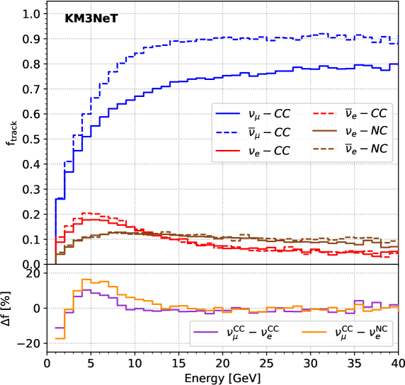
Figure 10: Fraction of events classified as track-like, $\text{f}_{\text{track}}$, with a CNN track probability $P_{i,\text{track}}>\text{0.5}$, for different interaction channels (top panel) versus the true MC neutrino energy. The relative improvement $\Delta\text{f}$, cf. Eq. 7.1, of the CNN with respect to the RF classifier in discriminating between ${}^{\text{CC}}$ events and shower-like ${}_{\text{e}}^{\text{CC}}$/ ${}_{\text{e}}^{\text{NC}}$ channels is shown in the bottom panel. Here, the contributions of neutrinos and antineutrinos are averaged for each flavour and interaction. The discrimination power is defined as the difference between the fractions of events classified as track-like and shower-like in the top panel.

It can be seen that the separation power between track-like and shower-like events depends on the neutrino energy. The CNN performs better than the RF in the energy range of roughly $3\text{\,}\mathrm{GeV}10\text{\,}\mathrm{GeV}$, while the RF performs better than the CNN for energies below $2\text{\,}\mathrm{GeV}$. As explained at the end of Sec. 6.4, this could again be due to limitations in the input images that become more relevant for events with only a few hits. Above $15\text{\,}\mathrm{GeV}$ the separation power of the two classifiers is roughly equal.

Since the performance comparison shown in Fig. 10 depends on the threshold value that is set for an event to be classified as track-like, another comparison metric independent of the threshold value is introduced. $P_{\text{track}}$ is defined as the probability that a classifier recognises a ${}^{\text{CC}}$ event as track-like, and similarly for ${}_{\text{e}}^{\text{CC}}$. Based on Fig. 9, the ability of a classifier to separate track-like and shower-like events can be estimated by calculating the energy-dependent correlation factor $c(E)$ of the two binned probability distributions $P_{i,\text{track}}(E)$ and $P_{i,\text{track}}^{{}_{\text{e}}}(E)$. The separability $S(E)$ is then given by:

$$S(E)=1-c(E)=1-\frac{\sum_{i}P_{i,\text{track}}(E)\cdot P^{{}_{\text{e}}}_{i,\text{track}}(E)}{\sqrt{\sum_{i}\left(P_{i,\text{track}}(E)\right)^{2}\cdot\sum_{i}\left(P^{{}_{\text{e}}}_{i,\text{track}}(E)\right)^{2}}}\,,$$ (7.2)

where the index $i$ in $P^{/{}_{\text{e}}}_{i,\text{track}}$ is the $i$-th bin of the distribution $P_{\text{track}}^{/{}_{\text{e}}}$ as shown in Fig. 9.

The separability $S(E)$ as a function of binned neutrino energy for the CNN and RF classifier is shown in Fig. 11. It is evident that the CNN-based classifier performs better by an absolute value of up to about 20% for energies below $10\text{\,}\mathrm{GeV}$. For these energies, the RF- and CNN-based classifier show both a better separability of ${}^{\text{CC}}$ and ${}_{\text{e}}^{\text{NC}}$ compared to ${}_{\text{e}}^{\text{CC}}$ events, although this loss in separability is less pronounced and reverses above $7\text{\,}\mathrm{GeV}$ for the RF classifier, i.e. at slightly lower energies than for the CNN classifier.

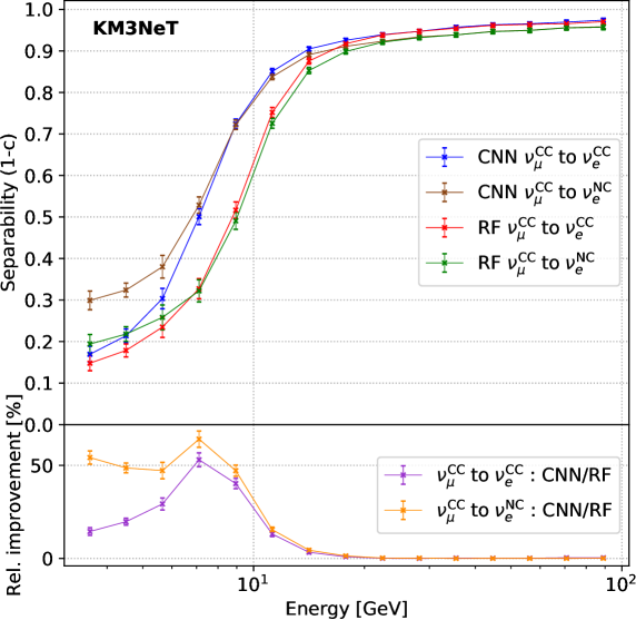
Figure 11: Separability $S(E)=1-c(E)$ based on ${}^{\text{CC}}$ and ${}_{\text{e}}^{\text{CC}}$ (${}^{\text{CC}}$ and ${}_{\text{e}}^{\text{NC}}$) events as a function of true MC neutrino energy for the CNN represented by blue (brown) markers and the RF represented by red (green) markers (top panel). Only (not $\mkern 1.5mu\overline{\mkern-1.5mu\upnu\mkern-1.5mu}\mkern 1.5mu$) have been used for the comparison. The relative improvement of the CNN with respect to the RF classifier in discriminating between ${}^{\text{CC}}$ events and shower-like ${}_{\text{e}}^{\text{CC/NC}}$ channels is shown in the bottom panel. The error bars indicate statistical errors only.

8 Event regression

This section introduces the CNN-based event regressor. The designed CNN now reconstructs continuous properties of the interacting neutrinos such as the direction, energy, the position of the interaction, i.e. the vertex, and an estimate for the uncertainty of each of these inferred observables. In the reconstruction pipeline for KM3NeT/ORCA as described in Ref. [2], these reconstruction tasks are handled by two maximum-likelihood-based algorithms optimised for track-like and shower-like events, respectively.

The major difference of the CNN for the regression task with respect to the classifiers in the previous sections is that its output is a continuous instead of a categorical variable.

8.1 Image generation

For the event regressor, the event images are created in a similar way to the image generation for the background and the track–shower classifier. Thus, both XYZT and XYZP images are produced and then stacked in the last dimension. Since the background classifier has already been applied to the data, at this final stage of the reconstruction pipeline neutrinos remain predominantly as input to the event regressor. Hence, exactly the same images as specified in Sec. 7 are used as input for the CNN event regressor.

8.2 Network architecture and loss functions

The network architecture of the CNN for the event regressor is similar to the one used for the background and track–shower classifier. However, for this work, it has been found that dropout layers in the CNN event regressor increase fluctuations in the training loss, even with a small dropout rate of $\delta=\text{0.05}$. Furthermore, the validation loss of the event regressor CNNs with dropout layers has proven to be significantly worse than for CNNs without dropout. Thus, no dropout layers are included. The fully-connected layers after the convolutional layers are also different. The properties that should be reconstructed by the network are the energy, the direction, and the vertex position of the initial neutrino interaction. For the direction and the vertex, the CNN output consists of two arrays with three elements each, containing the components of the vertex position vector and the direction cosines, respectively. Consequently, the output of the network consists of seven reconstructed floating-point numbers, denoted as $\vec{\upxi}_{\text{reco}}$, one component for the energy, three for the direction and three for the vertex position. The final fully-connected output layer therefore consists of seven neurons. The CNN architecture up to this point is shown in Tab. 5.

Building block / layer	Output dimension
XYZ-T Input	11 $\times$ 13 $\times$ 18	$\times$	60
XYZ-P Input	11 $\times$ 13 $\times$ 18	$\times$	31
Final stacked XYZ-T + XYZ-P Input	11 $\times$ 13 $\times$ 18	$\times$	91
Convolutional block 1 (64 filters)	11 $\times$ 13 $\times$ 18	$\times$	64
Convolutional block 2 (64 filters)	11 $\times$ 13 $\times$ 18	$\times$	64
Convolutional block 3 (64 filters)	11 $\times$ 13 $\times$ 18	$\times$	64
Convolutional block 4 (64 filters)	11 $\times$ 13 $\times$ 18	$\times$	64
Convolutional block 5 (64 filters)	11 $\times$ 13 $\times$ 18	$\times$	64
Convolutional block 6 (64 filters)	11 $\times$ 13 $\times$ 18	$\times$	64
Max pooling (2,2,2)	5 $\times$ 6 $\times$ 9	$\times$	64
Convolutional block 1 (128 filters)	5 $\times$ 6 $\times$ 9	$\times$	128
Convolutional block 2 (128 filters)	5 $\times$ 6 $\times$ 9	$\times$	128
Convolutional block 3 (128 filters)	5 $\times$ 6 $\times$ 9	$\times$	128
Convolutional block 4 (128 filters)	5 $\times$ 6 $\times$ 9	$\times$	128
Max pooling (2,2,2)	2 $\times$ 3 $\times$ 4	$\times$	128
Flatten	3072
Dense + ReLU	128
Dense + ReLU	32
Dense + Linear	7

Table 5: Network structure of the CNN event regressor with XYZ-T/P input, but without the additional fully-connected network for the uncertainty estimation. In the convolutional blocks and the last fully-connected layers no dropout layer is used.

Since the aim of this network is to reconstruct continuous variables, a categorical cross-entropy loss [20], as for the background and track–shower classifier, cannot be used. Instead, other cross-entropy-based loss functions can be employed, e.g. the mean squared error (MSE) or the mean absolute error (MAE) [20], which are defined as:

$$\text{MSE}=\frac{1}{n}\sum_{i=1}^{n}\left({}_{\text{reco}}-{}_{\text{true}}\right)^{2},$$ (8.1)

$$\text{MAE}=\frac{1}{n}\sum_{i=1}^{n}\left|{}_{\text{reco}}-{}_{\text{true}}\right|.$$ (8.2)

The main difference between the MSE and the MAE loss is that the MSE loss penalises outlier events that are badly reconstructed with a significantly larger loss value compared to the MAE loss. Since many detectable events are not fully contained in the KM3NeT/ORCA detector, these events are on average reconstructed more poorly. Thus, the MAE loss is used for the energy, direction and vertex estimation, so that the network focuses less on outlier events.
Using a neural network, it is also possible to estimate the uncertainties on the seven components of $\vec{\upxi}_{\text{reco}}$. One possibility is to let the network predict the absolute residual of the MAE loss. Thus, one needs an additional neuron that yields the estimated uncertainty, ${}_{\text{reco}}$, for each of the reconstructed components of $\vec{\upxi}_{\text{reco}}$. Consequently, the loss function that measures the quality of the estimated uncertainty value is:

$$L=\frac{1}{n}\sum_{i=1}^{n}\left({}_{\text{reco}}-\left|{}_{\text{true}}-{}_{\text{reco}}\right|\right)^{2}.$$ (8.3)

Using this loss function $L$, the network learns to estimate the average absolute residual:

$${}_{\text{reco}}\approx\left\langle\left|{}_{\text{true}}-{}_{\text{reco}}\right|\right\rangle.$$ (8.4)

Assuming that the residuals are normally distributed, the estimated uncertainty value ${}_{\text{reco}}$ can be converted to a standard deviation by multiplying by $\sqrt{\frac{\pi}{2}}$ [30].

In general, it can be expected that features that are learned by the convolutional part of the network and that are useful for the reconstruction are also crucial for the inference of the uncertainty on the reconstruction. Therefore, both inference tasks are handled by using the same CNN. The CNN, however, must be prevented from focusing too much on the uncertainty estimation in the learning process, since its main goal is the prediction of $\vec{\upxi}_{\text{reco}}$ and not of the uncertainties. For this purpose, a second fully-connected network with three layers is added after the convolutional output, but the gradient update during the back-propagation stage is stopped after the first fully-connected layer of this sub-network, as shown in Fig. 12.

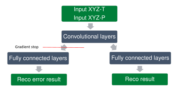
Figure 12: Scheme of the CNN architecture used for the event regressor. The properties of the convolutional layers and of the fully-connected network for the reconstruction of $\vec{\upxi}_{\text{reco}}$ is depicted in Tab. 5 and in Tab. 6.

The specific structure of the fully-connected network for the uncertainty reconstruction estimation is shown in Tab. 6.

Building block / layer	Output dimension
Dense + ReLU	128
Dense + ReLU	64
Dense + ReLU	32
Dense + Linear	7

Table 6: Layout of the fully-connected uncertainty reconstruction network, which is part of the event regressor CNN with XYZ-T/P input. The input to this dense network is the flattened output of the last convolutional layer of the main CNN.

8.3 Preparation of training, validation and test data

In order to train the CNN event regressor, again only simulated neutrino events are used. Similar to the track–shower classifier, the dataset consists of 50% track-like events (${}^{\text{CC}}$) and 50% shower-like events (25% ${}_{\text{e}}^{\text{CC}}$, 25% ${}_{\text{e}}^{\text{NC}}$). Additionally, the total dataset has been split again into a training, validation and test dataset. As for the track–shower classifier, the training data makes up 70%, the validation dataset 6% and the test dataset 24% of the total rebalanced dataset. The track and shower classes have not been balanced to be independent of neutrino energy, cf. Sec. 7.3, in order to get a larger training dataset compared to the track–shower classifier. In total, the training dataset then contains about $\text{14}\times\text{10}^{\text{6}}$ events.

The MC energy of ${}_{\text{e}}^{\text{NC}}$ events is set to the visible energy during the training, since the network cannot infer how much energy is carried away by the outgoing neutrino in the neutral current interaction.

Using a Nvidia Tesla V100 GPU, it takes about one and a half weeks to fully train this CNN event regressor.

8.4 Loss functions and loss weights

Before training the CNN event regressor, suitable loss weights need to be defined in order to scale the losses to the same magnitude. For example, the neutrino energy in the dataset ranges from $1\text{\,}\mathrm{GeV}100\text{\,}\mathrm{GeV}$, while the components of the direction vector range from $-1\text{\,}1\text{\,}$. Thus, the impact of the energy loss would be overwhelmingly large compared to the loss that is contributed by the direction reconstruction. Consequently, one needs to scale the individual losses of the components of $\vec{\upxi}_{\text{reco}}$ and their estimated uncertainties with a loss weight, such that all single losses are of the same order of magnitude at the start of the training. However, it has been observed that the CNN does not start to learn during the first few epochs of the training, if the individual losses of the energy, direction and vertex are of the same scale. The reason is that direction and vertex contribute six out of seven variables to be learned so that their impact on the total loss is dominant. Hence, any improvement with respect to the energy reconstruction, i.e. in the discrimination of background and signal hits, is marginalised by random statistical fluctuations in the loss for the direction or vertex components.

It is expected that the first concept the neural network will learn during the training is to distinguish signal and background hits. At the same time, the recognition of signal hits is a prerequisite for the direction and vertex reconstruction. Thus, the loss weights have been set in such a way that the scale of the energy loss at the start of the training is about two times larger than the scale of the three combined directional losses. For the same reason, the loss weights of the vertex reconstruction are set in such a way that they have the same scale as the directional losses. Indeed, it could be observed that the energy loss always converges significantly earlier during the training than the loss for the direction or vertex. Since the scale of the individual losses changes dramatically after the network has started to learn a property such as the energy or the direction, the loss weights need to be tuned during the training.

As a general strategy, it has proven useful to do this after the energy loss has sufficiently converged. How often and by how much the individual loss weights are retuned is a parameter optimisation process. For this work, the loss weights of the direction and vertex components have been increased by a factor of three after the energy loss convergence, and, at the end of the training, these loss weights have been doubled again to investigate if further improvements would occur, which was not the case. Increasing the weights for the direction and vertex losses did not significantly worsen the energy loss.

For the loss weights of the uncertainty outputs none of this matters, since their gradients are stopped after the first fully-connected layer of the uncertainty reconstruction sub-network. Thus, the loss weights for these variables just need to be set such that the scale of the individual losses is about the same.

8.5 Energy reconstruction performance

In this section the neutrino energy reconstruction performance of the CNN event regressor is investigated. The study and the comparisons to the maximum-likelihood-based reconstruction algorithm, described in Ref. [2] and called SOR in the following, focus on shower-like events.

Events have been selected according to the criteria detailed in Sec. 6.4. In particular, only events reconstructed as up-going by the SOR algorithm are selected for the comparison and, additionally, the vertex position, direction, and energy of true ${}_{\text{e}}^{\text{CC}}$ events must have been reconstructed with high confidence by SOR.

The reconstructed energy versus the true MC energy for reconstructed ${}_{\text{e}}^{\text{CC}}$ events is shown in Fig. 13.

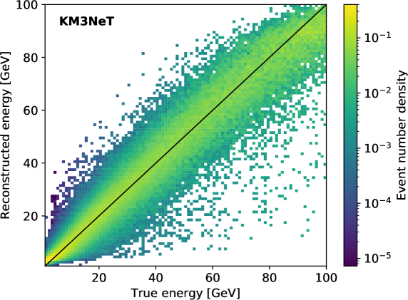
Figure 13: Energy reconstructed by the CNN regressor versus true MC neutrino energy for reconstructed ${}_{\text{e}}^{\text{CC}}$ events. The distribution has been normalised to unity in each true energy bin.

As can be seen in the figure, the energy reconstruction tends to underestimate the true MC energy of the neutrino, in particular for energies above $30\text{\,}\mathrm{GeV}$. This effect has been found to be even more evident for SOR, so that a correction function has been applied to the reconstructed energy. This correction function has been derived from MC simulations and depends on several reconstructed quantities, such as the energy, the zenith angle, and the interaction inelasticity (Sec. D.1. in Ref. [31]). So as to allow for a comparison between the SOR algorithm and the CNN event regressor, a similar but simpler correction function, only using the reconstructed energy, has been derived and applied to the energy reconstruction of the CNN event regressor for ${}_{\text{e}}^{\text{CC}}$ events. The resulting distributions can be compared in Fig. 14.

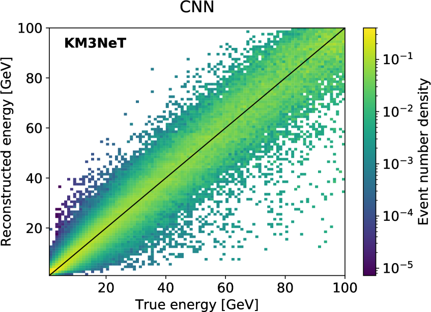
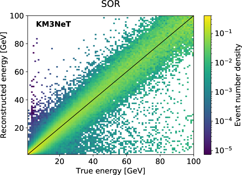
Figure 14: Reconstructed and corrected energy versus true MC neutrino energy for reconstructed ${}_{\text{e}}^{\text{CC}}$ events. The distribution has been normalised to unity in each true energy bin. Left: CNN event regressor. Right: Maximum-likelihood-based reconstruction algorithm SOR for shower-like events as described in Ref. [2].

In order to allow for quantitative comparisons, the following two performance metrics are used: the median relative error (MRE) and the relative standard deviation (RSD). Both metrics are calculated for each MC energy bin. The MRE is defined as:

$$\text{MRE}=\text{Median}\left(\left|\frac{\text{E}_{\text{reco}}-\text{E}_{\text{true}}}{\text{E}_{\text{true}}}\right|\right)\,,$$ (8.5)

where $\text{E}_{\text{reco}}$ ($\text{E}_{\text{true}}$) stands for the reconstructed (true MC) energy.

For the RSD, the standard deviation of the reconstructed energy distribution for each MC true energy bin is calculated and then divided by the energy of the bin:

$$\text{RSD}=\frac{\upsigma}{\text{E}_{\text{true}}}.$$ (8.6)

For shower-like events, the energy reconstruction performance is intrinsically limited by light yield fluctuations of the hadronic particle cascade [5]. Assuming that both the CNN event regressor and the SOR algorithm come close to this intrinsic resolution limit, it is to be expected that the MRE and RSD performances for both methods agree very well, as can be seen in Fig. 15 (left) and Fig. 15 (right), respectively. For the MRE, the CNN shows lower values than the SOR algorithm for energies close to the boundaries of the investigated energy range. This is due to the fact that the CNN learns the limits of the simulated neutrino energy spectrum, i.e. $1\text{\,}\mathrm{GeV}$ and $100\text{\,}\mathrm{GeV}$. Therefore, the CNN, contrary to the SOR algorithm, never reconstructs energies outside of this energy range, which biases the MRE for the CNN towards lower values. For the high-energy boundary, this effect can be easily avoided by extending the simulated energy range. For the low-energy boundary, this is not easily possible and biases the comparison with the SOR algorithm, albeit only in an energy range that is close to the detection energy threshold of KM3NeT/ORCA. On the other hand, it is notable that the RSD for the CNN event regressor improves by a few percent with respect to the SOR algorithm also for energies far from the boundaries.

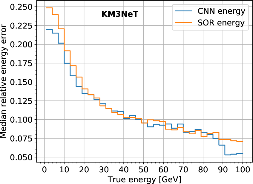
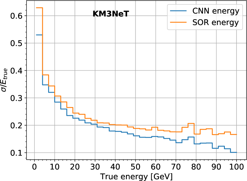
Figure 15: Left: Median relative error (MRE) on the reconstructed energy versus true MC energy for ${}_{\text{e}}^{\text{CC}}$ events for the CNN event regressor (blue) and SOR (orange). Right: Relative standard deviation (RSD) on the reconstructed energy versus true MC energy for the CNN event regressor (blue) and SOR (orange).

In the case of ${}_{\text{e}}^{\text{NC}}$ events, the energy reconstruction performance is limited by the non-detectable energy that is carried away by the outgoing neutrino. For ${}_{\text{e}}^{\text{NC}}$ events, as for charged-current events, the energy reconstruction performance of the CNN event regressor and SOR is similar.

8.6 Direction reconstruction performance

The direction reconstruction performance of the CNN event regressor is investigated in the same way as for the energy reconstruction. The X, Y and Z components of the reconstructed direction vector are converted to spherical azimuth and zenith coordinates. Since the DUs, cf. Sec. 2.1, are approximately vertical structures, the azimuth angle is defined by the projection of the direction vector onto a plane roughly perpendicular to the DUs, while the zenith roughly corresponds to the angle enclosed by the direction vector pointing back to the particle’s source and the DUs.

The median absolute error (ME) is defined as the median of the distribution of ${}_{\text{reco}}-{}_{\text{true}}$. In Fig. 16 the ME for the azimuth and the zenith angle of the reconstructed direction is compared for the CNN event regressor and SOR. The comparison is done for ${}_{\text{e}}^{\text{CC}}$ events and as a function of the true MC neutrino energy.

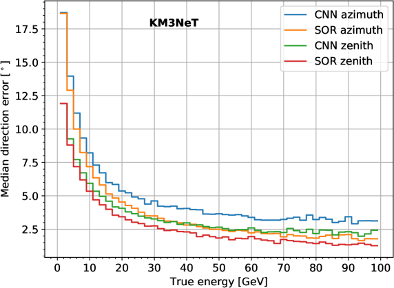
Figure 16: Median absolute error of the zenith and azimuth angle reconstruction for the CNN event regressor and the shower reconstruction algorithm SOR versus true MC energy for ${}_{\text{e}}^{\text{CC}}$ events.

For energies below $3\text{\,}\mathrm{GeV}$, the ME is very similar for both reconstructions, while the difference in performance increases in favour of the SOR algorithm with increasing energy. At $20\text{\,}\mathrm{GeV}$, the ME for the reconstruction of the neutrino zenith (azimuth) angle is about 15% (25%) larger for the CNN event regressor than for SOR. The reason for this worse performance of the CNN might be connected to the rather coarse time binning chosen for the image generation. The corresponding comparison for ${}_{\text{e}}^{\text{NC}}$ events shows the same general trend, but the performance gap is smaller since the reconstruction is intrinsically limited by the interaction kinematics.

8.7 Vertex reconstruction performance

For the comparison of the vertex reconstruction performance the distance between the reconstructed and the true MC vertex point is investigated based on the longitudinal and perpendicular components of the residual vector with respect to the direction of the incoming neutrino. The CNN event regressor is trained such that it reconstructs the neutrino interaction vertex, while the SOR algorithm reconstructs the brightest point of the Cherenkov light emission, which is shifted by an energy-dependent displacement of the order of meters.

The perpendicular versus longitudinal distance of the reconstructed vertex with respect to the true ${}_{\text{e}}^{\text{CC}}$ interaction point is shown in Fig. 17 (left) for the CNN event regressor, while the right plot shows the same distribution for the SOR algorithm. The above mentioned displaced reconstruction of the brightest emission point can be seen for the SOR algorithm in Fig. 17 (right). The CNN-based vertex resolution is of the order of one meter with a small offset in perpendicular direction in the investigated energy range up to $100\text{\,}\mathrm{GeV}$. For the SOR algorithm, the resolution in the longitudinal direction is similar, while it is better in the perpendicular direction. A correlation of longitudinal and perpendicular errors can be seen for the SOR algorithm, which is absent for the CNN reconstruction.

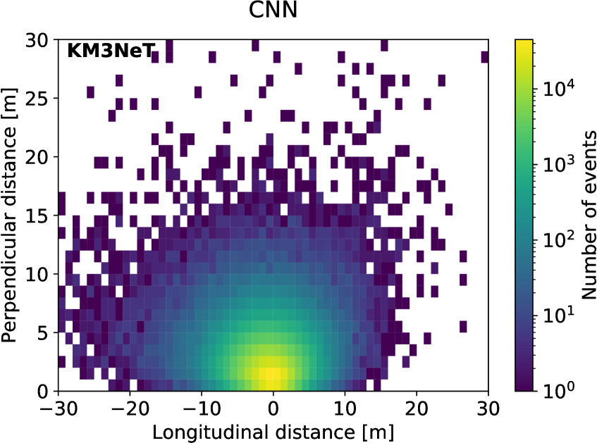
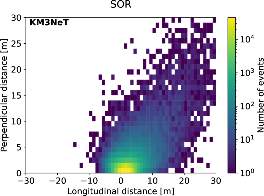
Figure 17: Reconstructed neutrino interaction point with respect to the true MC vertex for ${}_{\text{e}}^{\text{CC}}$ events. Shown is the perpendicular component versus the longitudinal component of the distance vector. Left: CNN event regressor; Right: SOR algorithm.

8.8 Error estimation

The CNN is used to reconstruct the regression uncertainty of all reconstructed quantities, as explained in Sec. 8.2. For the following performance investigation the event pre-selection, based on the current KM3NeT/ORCA reconstruction pipeline, is not applied, i.e. all triggered events of the simulated test dataset are used. In order to evaluate the goodness of the uncertainty reconstruction for any event quantity, e.g. energy or direction, the events are binned according to their estimated uncertainty value, ${}_{\text{reco}}$. For the event distribution in each bin, the standard deviation, ${}_{\text{true}}$, of the residuals of the reconstructed and true MC values $\left|{}_{\text{reco}}-{}_{\text{true}}\right|$ is calculated.

The distribution of ${}_{\text{true}}$ versus ${}_{\text{reco}}$ is shown in Fig. 18 (left) for the energy reconstruction of ${}_{\text{e}}^{\text{CC}}$ events. Even though ${}_{\text{reco}}$ is estimated with a significant fraction of events that were discarded previously by the criteria applied for the energy reconstruction in Sec. 8.5, the CNN event regressor estimation of the reconstruction uncertainty is clearly correlated to the true uncertainty. As can be seen, the energy uncertainty is slightly underestimated for events that are difficult to reconstruct and therefore show large estimated uncertainties.

The distribution of ${}_{\text{true}}$ versus ${}_{\text{reco}}$ is shown in Fig. 18 (right) for the Z component of the reconstructed direction vector in ${}_{\text{e}}^{\text{CC}}$ events. In the range of $\text{0.15}<{}_{\text{reco}}<\text{0.30}$ a slight underestimation in the uncertainty reconstruction can be seen.

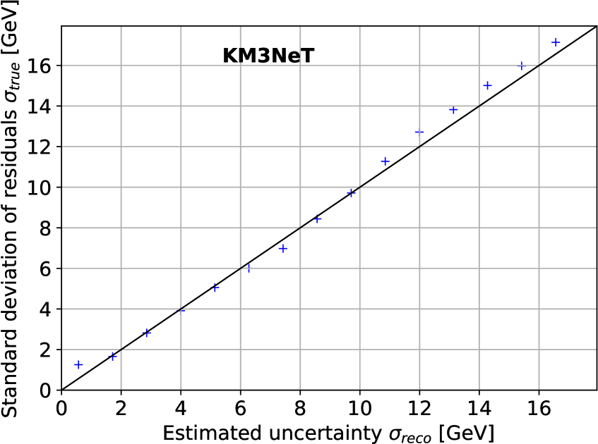
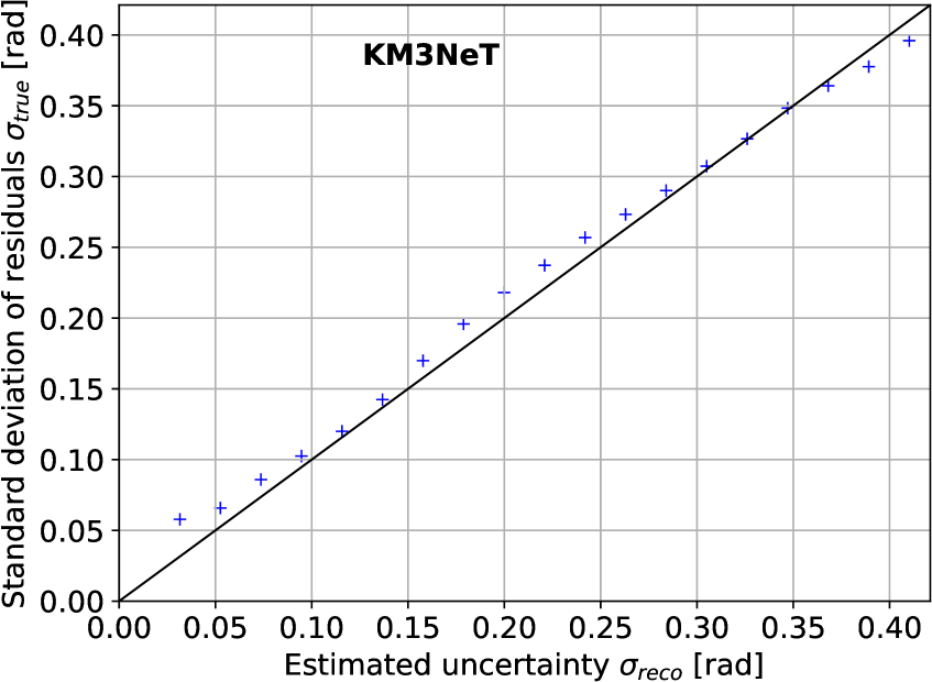
Figure 18: Standard deviation of the difference of true MC and reconstructed values versus the uncertainty estimated by the CNN event regressor. Left: for the energy reconstruction of ${}_{\text{e}}^{\text{CC}}$ events. Right: for the Z component of the reconstructed direction vector for ${}_{\text{e}}^{\text{CC}}$ events.

Since there is a clear correlation between the predicted and the true uncertainty, it is possible to discriminate badly reconstructed events based on the estimated uncertainty value ${}_{\text{reco}}$. In order to demonstrate this, the zenith-angle reconstruction for shower-like events is investigated. The standard deviation of the residual distribution of the reconstructed cosine of the zenith angle for ${}_{\text{e}}^{\text{CC}}$ events versus the fraction of events discarded by the CNN uncertainty estimator is depicted in Fig. 19. For all three energy intervals depicted, one can see that the zenith-angle resolution improves significantly when the events are discarded, that have the largest reconstruction errors as predicted by the CNN.

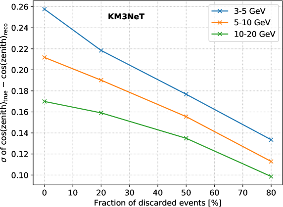
Figure 19: Standard deviation of the residual distribution of the reconstructed cosine of the zenith angle for ${}_{\text{e}}^{\text{CC}}$ versus the fraction of events discarded by the CNN uncertainty estimator. The neutrino events have been generated in three different energy intervals as indicated by the three coloured lines.

9 Conclusion

In this work, the first application of deep convolutional neural networks to the reconstruction and classification of simulated neutrino events in the neutrino detector KM3NeT/ORCA has been reported. Detailed MC datasets have been suitably pre-processed to generate pixelated high-dimensional image input for the training of CNNs. CNNs have been designed to separate neutrino events from background, and track-like from shower-like neutrino events. In addition, CNNs have been used to reconstruct the direction, energy, and interaction point of the neutrinos, and to estimate the uncertainty on each of the reconstructed quantities. Comparisons to the performance of classical machine-learning approaches to classification and maximum-likelihood reconstructions show the competitive and in some cases already superior performance of the employed CNNs, though there are still many aspects that can possibly be optimised. In the next step, the developed CNNs will be tested for robustness with respect to real data acquisition conditions, e.g. for the effect of missing optical modules and imperfect calibrations, before they will be applied to data taken with the KM3NeT/ORCA detector.

References

- [1] M. Ageron et al., ANTARES: the first undersea neutrino telescope, Nucl. Instrum. Meth. A656 (2011) 11–38.
- [2] S. Adrián-Martínez et al., Letter of Intent for KM3NeT 2.0, J. Phys. G43 (2016) 084001.
- [3] E. Kh. Akhmedov, S. Razzaque and A. Yu Smirnov, Mass hierarchy, 2-3 mixing and CP-phase with huge atmospheric neutrino detectors, JHEP 2 (2013) 82.
- [4] M. Tanabashi et al., Review of Particle Physics, Phys. Rev. D98 (2018) 030001.
- [5] S. Adrián-Martínez et al., Intrinsic limits on resolutions in muon- and electron-neutrino charged-current events in the KM3NeT/ORCA detector, JHEP 5 (2017) 8.
- [6] L. Breiman, Random Forests, Machine Learning 45 (2001) 5–32.
- [7] O. Russakovsky et al., ImageNet Large Scale Visual Recognition Challenge, Int. J. Comput. Vis. 115 (2015) 211–252.
- [8] ImageNet: Where have we been? Where are we going?, URL: http://image-net.org/challenges/talks_2017/imagenet_ilsvrc2017_v1.0.pdf.
- [9] D. Guest, K. Cranmer and D. Whiteson, Deep Learning and its Application to LHC Physics, Ann. Rev. Nucl. Part. Sci. 68 (2018) 161–181.
- [10] I. Shilon et al., Application of Deep Learning methods to analysis of Imaging Atmospheric Cherenkov Telescopes data, Astropart. Phys. 105 (2019) 44–53.
- [11] M. Erdmann, J. Glombitza, and D. Walz, A Deep Learning-based Reconstruction of Cosmic Ray-induced Air Showers, Astropart. Phys. 97 (2018) 46–53.
- [12] M. Hünnefeld, Deep Learning in Physics exemplified by the Reconstruction of Muon-Neutrino Events in IceCube, PoS 35th International Cosmic Ray Conference 301 (2017).
- [13] A. Aurisano et al., A Convolutional Neural Network Neutrino Event Classifier, JINST 11 (2016) P09001.
- [14] F. Chollet et al., Keras, URL: https://keras.io.
- [15] M. Moser and S. Reck, OrcaNet, URL: https://github.com/KM3NeT/OrcaNet.
- [16] M. Ageron et al., Dependence of atmospheric muon flux on seawater depth measured with the first KM3NeT detection units, Eur. Phys. J. C80 (2020) 99.
- [17] M. Honda et al., Atmospheric neutrino flux calculation using the NRLMSISE-00 atmospheric model, Phys. Rev. D92 (2017) 023004.
- [18] G. Carminati, A. Margiotta and M. Spurio, Atmospheric MUons from PArametric formulas: A Fast GEnerator for neutrino telescopes (MUPAGE), Comput. Phys. Commun. 179 (2008) 915–923.
- [19] Stanford University, Lecture notes on Convolutional Neural Networks for Visual Recognition (2016), URL: http://cs231n.github.io/convolutional-networks.
- [20] I. Goodfellow, Y. Bengio and A. Courville, Deep Learning, MIT Press (2016).
- [21] N. Srivastava et al., Dropout: A Simple Way to Prevent Neural Networks from Overfitting, J. Mach. Learn. Res. 15 (2014) 1929–1958.
- [22] S. Aiello et al., Characterisation of the Hamamatsu photomultipliers for the KM3NeT Neutrino Telescope, JINST 13 (2018) P05035.
- [23] M. Abadi et al., TensorFlow: Large-Scale Machine Learning on Heterogeneous Systems, URL: http://tensorflow.org.
- [24] S. Ioffe and C. Szegedy, Batch Normalization: Accelerating Deep Network Training by Reducing Internal Covariate Shift, ICML’15: Proceedings of the 32nd International Conference on International Conference on Machine Learning 37 (2015).
- [25] S. Santurkar et al., How Does Batch Normalization Help Optimization?, NeurIPS’18: 32nd Conference on Neural Information Processing Systems (2018).
- [26] K. He et al., Delving Deep into Rectifiers: Surpassing Human-Level Performance on ImageNet Classification, ICCV’15: Proceedings of the 2015 IEEE International Conference on Computer Vision (2015).
- [27] D. P. Kingma and J. Ba, Adam: A Method for Stochastic Optimization, ICLR’15: International Conference on Learning Representations (2015).
- [28] Tensorflow API documentation, URL: https://www.tensorflow.org/api_docs/python/tf/train/AdamOptimizer.
- [29] J. Nickolls et al., Scalable Parallel Programming with CUDA, Queue 6 (2008) 40–53.
- [30] R. C. Geary, The ratio of the mean deviation to the standard deviation as a test of normality, Biometrika 27 (1935) 3–4.
- [31] J. Hofestädt, doctoral thesis, Performance studies for the ORCA neutrino detector, Friedrich-Alexander-Universität Erlangen–Nürnberg (FAU) (2017).