A Survey of Approximate Quantile Computation on Large-scale Data (Technical Report)

Abstract

As data volume grows extensively, data profiling helps to extract metadata of large-scale data. However, one kind of metadata, order statistics, is difficult to be computed because they are not mergeable or incremental. Thus, the limitation of time and memory space does not support their computation on large-scale data. In this paper, we focus on an order statistic, quantiles, and present a comprehensive analysis of studies on approximate quantile computation. Both deterministic algorithms and randomized algorithms that compute approximate quantiles over streaming models or distributed models are covered. Then, multiple techniques for improving the efficiency and performance of approximate quantile algorithms in various scenarios, such as skewed data and high-speed data streams, are presented. Finally, we conclude with coverage of existing packages in different languages and with a brief discussion of the future direction in this area.

I Introduction

Data profiling is a set of activities to describe the metadata about given data [1, 2]. It is crucial for data analysis, especially for large-scale data. It helps researchers to understand data distribution [3], discover duplicates [4, 5], detect anomalies [6], determine thresholds [7, 8], etc. Such information provides guidance for other data preprocessing work such as data cleaning [9, 10], which can subsequently improve the performance of data mining dramatically [11]. When preprocessing large-scale data, data profiling is attached great importance to and faces its own challenges. Because of large data size, classic brutal methods are not applicable any more for their intolerable complexity of both time and space. Researchers have spent decades on figuring out new ways to compute the metadata which can be calculated easily on small data. The metadata can be divided into two categories based on scalability: aggregation statistics and order statistics [12].

Aggregation statistics are named for their property that they are mergeable and incremental, which makes them relatively easy to be computed no matter how large the data is. For examples, sum, mean values, standard deviations, min or max values are all aggregation statistics. For streaming models [13, 14], where data elements come one by one with time, we can trace and update aggregated results covering all arrived data by incrementing new results continuously. Time complexity and space complexity are both $O(1)$. As for distributed models [15], where data are stored in nodes of a distributed network, the overall aggregation statistics can be obtained by merging results from each node. The total communication cost of this computation is $O(|v|)$, where $|v|$ is the number of network nodes. However, order statistics, such as quantiles, heavy hitters, etc., do not preserve such property. So, we cannot compute them by merging existing results with newly produced results in a straight way. In order to compute them, many customized data structures or storage structures are proposed for these order statistics, trying to turn them into a mergeable or incremental form in some way.

In this summary, we focus on one order statistic, quantiles. They help to generate the description of the data distributions without parameters. In other words, they are able to reflect the cumulative distribution function (cdf), thus the probability distribution function (pdf), of data at low computational cost. Pdf is widely used in data cleaning and data querying. For example, in data cleaning, it is applied to demonstrate the distance distribution among values of the same attribute so as to identify misplaced attribute values [16]. And in data querying, it helps to set an appropriate correlation filter, improving efficiency for set correlation query over set records in databases [17]. Therefore, quantiles are regarded as one of the most fundamental and most important statistics in data quality analysis in both theory and practice. For instance, many data analysis tools, including Excel, MATLAB, Python, etc., have quantile-computing functions as built-in components or libraries. In the Sawzall language, which is the basic for all Google’s log data analysis, quantile is one of the seven basic statistic operators defined, along with sum, max, top-k, etc. [18]. Besides, quantiles are widely used in data collection and running-state monitoring in sensor networks [19, 20]. When a dataset contains dirty values, compared with mean values and standard deviations, quantiles and median absolute deviations are more objective and more accurate to reflect data center and data deviation [21]. They are less sensitive to outliers. In temporal data, where imprecise timestamps are prevalent, even if some timestamps are delayed very long or have inconsistent granularity, quantiles are still able to specify appropriate temporal constraints on time interval, helping to clean the data [22]. In addition, quantile algorithms have been widely used as subroutines to resolve more complicated problems, such as equi-depth histograms [23] and dynamic geometric computations [24].

A quantile is the element at a certain rank in the dataset after sort. Algorithmic studies can be traced back to 1973 at least when linear-time selection was invented [25]. In classic methods of computing $\phi$-quantile over a dataset of size $N$, where $\phi\in(0,1)$, first we sort all elements and then return the one ranking $\lfloor\phi{N}\rfloor$. Its time complexity is $O(N\log{N})$ and space complexity is $O(N)$ obviously. However, in large-scale data, the method is infeasible under restrictions of memory size. Munro et al. has proved that any exact quantile algorithm with $p$-pass scan over data requires at least $\Omega(N^{1/p})$ space [26]. Besides, in streaming models, e.g., over streaming events [27], quantile algorithms should also be streaming. That is, they are permitted to scan each element only once and need to update quantile answers instantaneously when receiving new elements. There is no way to compute quantiles exactly under such condition. Thus, approximation is introduced in quantile computation. Approximate computation is an efficient way to analyze large-scale data under restricted resources [28]. On one hand, it raises computational efficiency and lower computational space. On the other hand, large scale of the dataset can dilute approximation effects. Large-scale data is usually dirty, which also makes approximate quantile endurable and applicable in industry. Significantly, the scale of data is relative, based on the availability of time and space. So, the rule about how to choose between exact quantiles and approximate quantiles differs in heterogeneous scenarios, depending on the requirement for accuracy and the contradiction between the scale of data and that of resources. When the cost of computing exact quantiles is intolerable and the results are not required to be totally precise, approximate quantiles are a promising alternative.

We denote approximation error by $\epsilon$. A $\epsilon$-approximate $\phi$-quantile is any element whose rank is between $r-\epsilon{N}$ and $r+\epsilon{N}$ after sort, where $r=\lfloor\phi{N}\rfloor$. For example, we want to calculate $0.1$-approximate $0.3$-quantile of the dataset ${11,21,24,61,81,39,89,56,12,51}$. As shown in Figure 1, we sort the elements as ${11,12,21,24,39,51,56,61,81,89}$ and compute the range of the quantile’s rank, which is $[(0.3-0.1)\times 10,(0.3+0.1)\times 10]=[2,4]$. Thus the answer can be one of ${12,21,24}$. In order to further reduce computation space, approximate quantile computation is often combined with randomized sampling, making the deterministic computation becomes randomized. In such case, another parameter $\delta$, or randomization degree, is introduced, meaning the algorithm answers a correct quantile with a probability of at least $1-\delta$.

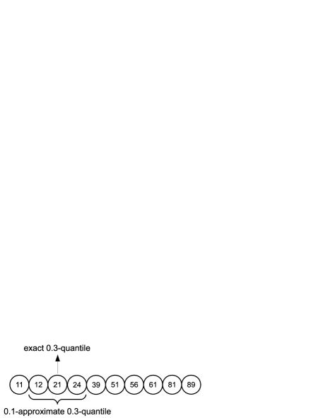
Figure 1: An example of a $\epsilon$-approximate $\phi$-quantile, where $\epsilon=0.1$ and $\phi=0.3$.

There are 3 basic metrics to assess an approximate quantile algorithm [29]:

• Space complexity It is necessary for streaming algorithms. Due to the limitation of memory, only algorithms using sublinear space are applicable [30]. It corresponds to communication cost in distributed models. In a distributed sensor network, communication overhead consumes more power and limits the battery life of power-constrained devices, such as wireless sensor nodes [31]. So, quantile algorithms are aimed at low space complexity or low communication cost.

• Update time It is the time spent on updating quantile answers when new element arrives. Fast updates can improve the user experience, so many streaming algorithms take update time as a main consideration.

• Accuracy It measures the distance between approximate quantiles and ground truth. Intuitively, the more accurate an algorithm is, the more space and the longer time it will consume. They are on the trade-off relationship. We use approximation error, maximum actual approximation error and average actual approximation error as quantitative indicators to measure accuracy.

We collected and studied researches about approximate quantile computation, then completed this survey. The survey includes various algorithms, varying from data sampling to data structure transformation, and techniques for optimization. Important algorithms are listed in Table I. The remaining parts of this survey are organized as follows: In Section II, we introduce deterministic quantile algorithms over both streaming models and distributed models. Section III discusses randomized algorithms [32]. Section IV introduces some techniques and algorithms for improving the performance and efficiency of quantile algorithms in various scenarios. Section V presents a few off-the-shelf tools in industry for quantile computation. Finally, Section VI makes the conclusion and proposes interesting directions for future research.

TABLE I: Approximate quantile algorithms

Algorithm	Randomization	Model	Space complexity / Communication cost
MRL98 [33]	Deterministic	Streaming	$O(\frac{1}{\epsilon}\log^{2}(\epsilon{N}))$
GK01 [34]	Deterministic	Streaming	$O(\frac{1}{\epsilon}\log(\epsilon{N}))$
Lin SW [35]	Deterministic	Streaming	$O(\frac{1}{\epsilon}\log(\epsilon^{2}N)+\frac{1}{\epsilon^{2}})$
Lin n-of-N [35]	Deterministic	Streaming	$O(\frac{1}{\epsilon^{2}}\log^{2}(\epsilon{N}))$
Arasu FSSW [36]	Deterministic	Streaming	$O(\frac{1}{\epsilon}\log\frac{1}{\epsilon}\log{N})$
Arasu VSSW [36]	Deterministic	Streaming	$O(\frac{1}{\epsilon}\log\frac{1}{\epsilon}\log(\epsilon{N})\log{N})$
GK-UN [37]	Deterministic	Streaming	$O(\frac{1}{\epsilon}\log(\epsilon{PC(S^{u})}))$
Q-digest [20]	Deterministic	Distributed	$O(\frac{1}{\epsilon}|v|\log\sigma)$
GK04 [38]	Deterministic	Distributed	$O(\frac{|v|}{\epsilon}\log^{2}{N})$
Cormode05 [39]	Deterministic	Distributed	$O(\frac{|v|}{\epsilon^{2}}\log{N})$
Yi13 [40]	Deterministic	Distributed	$O(\frac{|v|}{\epsilon}\log{N})$
MRL99 [41]	Randomized	Streaming	$O(\frac{1}{\epsilon}\log^{2}\frac{1}{\epsilon})$
Agarwal13 [42]	Randomized	Streaming	$O(\frac{1}{\epsilon}\log^{1.5}\frac{1}{\epsilon})$
Felber15 [43]	Randomized	Streaming	$O(\frac{1}{\epsilon}\log\frac{1}{\epsilon})$
Karnin16 [44]	Randomized	Streaming	$O(\frac{1}{\epsilon}\log\log\frac{1}{\epsilon\delta})$
Huang11 [45]	Randomized	Distributed	$O(\frac{1}{\epsilon}\sqrt{|v|h})$
Haeupler18 [46]	Randomized	Distributed	$O(\log\log{N}+\log\frac{1}{\epsilon})$

II Deterministic Algorithms

An algorithm is deterministic while it returns a fixed answer given the same dataset and query condition. Furthermore, quantile algorithms are classified based on their application scenarios. In streaming models, where data elements arrive one by one in a streaming way, algorithms are required to answer quantile queries with only one-pass scan, given the data size $N$ [33] or not [47, 48, 34, 36, 37]. Except to answering quantile queries for all arrived data, Lin et al. [35] concentrates on tracing quantiles for the most recent $N$ elements over a data stream. In distributed models, where data or statistics are stored in distributed architectures such as sensor networks, algorithms are proposed to merge quantile results from child nodes using as low communication cost as possible to reduce energy consumption and prolong equipment life [20, 38, 45, 42, 40].

II-A Streaming Model

The most prominent feature of streaming algorithms is that all data are required to be scanned only once. Besides, the length of the data stream may be uncertain and can even grow arbitrarily large. Thus, classic quantile algorithms are infeasible for streaming models because of the limitation of memory. Therefore, the priority of approximate quantile algorithms for streaming models is to minimize space complexities. In 2010, Hung et al. [49] have proved that any comparison-based $\epsilon$-approximate quantile algorithm over streaming models needs space complexity of at least $\Omega(\frac{1}{\epsilon}\log\frac{1}{\epsilon})$, which sets a lower bound for these algorithms.

Both Jain et al. [50] and Agrawal et al. [51] proposed algorithms to compute quantiles with one-pass scan. However, neither of them clarified the upper or lower bound of approximation error. In 1997, Alsabti et al. [47] improved the algorithm and came up with a version with guaranteed error bound, referred to as ARS97. Its basic idea is sampling and it includes the following steps:

1. Divide the dataset into $r$ partitions.

2. For each partition, sample $s$ elements and store them in a sorted way.

3. Combine $r$ partitions of data, generating one sequence for querying quantiles.

ARS97 is targeted at disk-resident data, rather than streaming models. Nevertheless, its idea to partition the entire dataset and maintain a sampled sorted sequence for quantile querying inspires quantile algorithms over streaming models afterwards.

The inspired algorithm is referred to as MRL98 proposed by Manku et al. [33]. It requires the prior knowledge of the length $N$ of data stream. Similar with ARS97, MRL98 divides the data stream into $b$ blocks, samples $k$ elements from each block and puts them into $b$ buffers. Each buffer $X$ is given a weight $w(X)$, representing the number of elements covered by this buffer. The algorithm consists of 3 operations:

• NEW Put the first $bk$ elements into buffers successively and set their weights to $1$.

• COLLAPSE Compress elements from multiple buffers into one buffer. Specifically, each element from an input buffer $X_{i}$ would be duplicated $w(X_{i})$ times. Then these duplicated elements are sorted and merged into a sequence, where $k$ elements are selected at regular intervals and stored in the output buffer $Y$, whose weight $w(Y)=\sum_{i}{w(X_{i})}$

• OUTPUT Select an element as the quantile answer from $b$ buffers.

NEW and OUTPUT are straightforward, so the algorithm’s space complexity depends mainly on how to trigger COLLAPSE. MRL98 proposed a tree-structure trigger strategy. Each buffer $X$ is assigned a height $l(X)$ and $l$ is set to $min_{i}{l(X_{i})}$. $l(X)$ is set as the following standard:

• If only one buffer is empty, its height is set to $l$.

• If there are two or more empty buffers, their heights are set to $0$.

• Otherwise, buffers of height $l$ are collapsed, generating a buffer of height $l+1$.

By tuning $b$ and $k$, MLR98 can narrow the approximation error within $\epsilon$. Figure 2 demonstrates the trigger strategy when $b=3$. The height of the strategy tree is logarithmic, thus the space complexity is $O(\frac{1}{\epsilon}\log^{2}(\epsilon{N}))$.

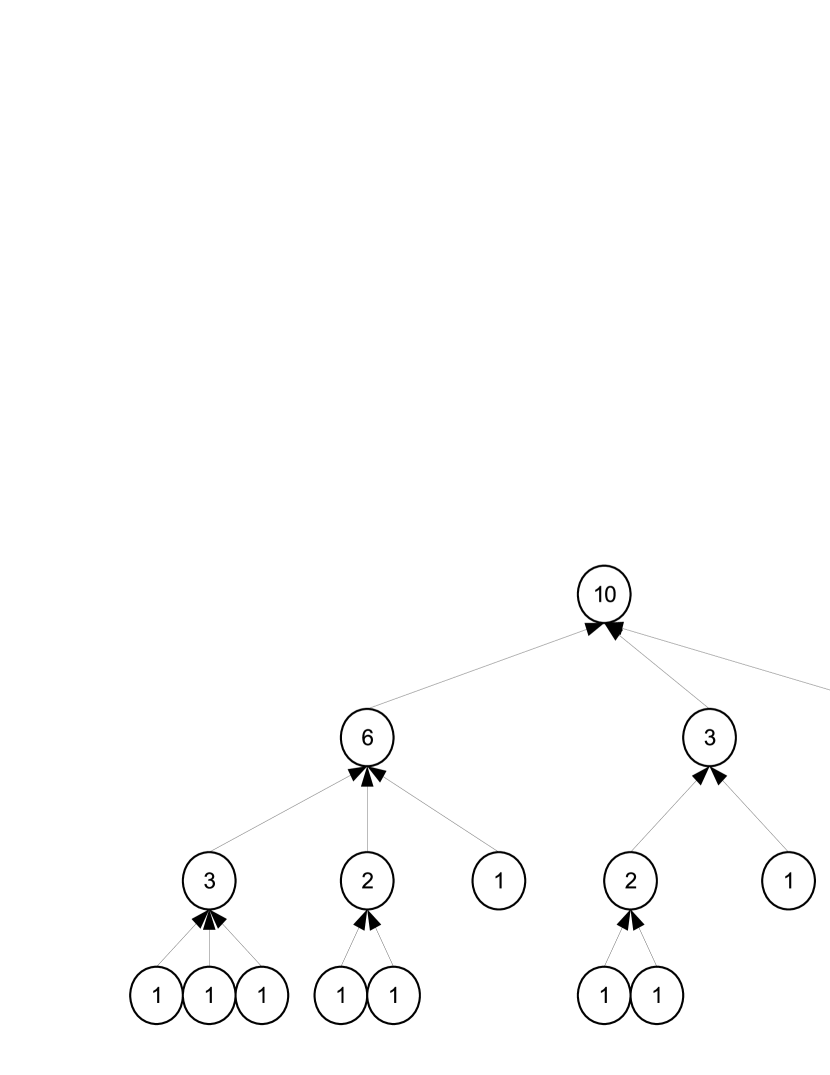
Figure 2: The collapsing strategy with 3 buffers. A node corresponds to a buffer and its number denotes the weight.

The limitation of MRL98 is that it needs to know the length of the data stream at first. However, in more cases, the length is uncertain and may even grow arbitrarily large. In such case, Greenwald et al. [34] proposes celebrated GK01 algorithm, distinguished by its innovative data structure, $Summaries$, or $S$ for short. The basic idea is that when $N$ increases, the set of $\epsilon$-approximate answers for querying $\phi$-quantile expands as well, so correctness can be retained even if removing some elements. $S$ is a collection of tuples in the form of $(v_{i},g_{i},\Delta_{i})$, where $v_{i}$ is the element with the property $v_{i}\leq v_{i+1}$, $g_{i}$ and $\Delta_{i}$ are $2$ integers satisfying following conditions:

$$\sum_{j\leq i}g_{j}\leq r(v_{i})+1\leq\sum_{j\leq i}g_{j}+\Delta_{i}$$ (1)

$$g_{i}+\Delta_{i}\leq\lfloor 2\epsilon{N}\rfloor$$ (2)

$r(v_{i})$, whose bounds are guaranteed by (1), is the ground truth of $v_{i}$’s rank. Obviously, there are at most $g_{i}+\Delta_{i}-1$ elements between $v_{i-1}$ and $v_{i}$. (2) makes sure that the range is within $\lfloor 2\epsilon{N}\rfloor-1$. Therefore, for any $\phi\in(0,1)$, there always exists a tuple $(v_{i},g_{i},\Delta_{i})$, where $r(v_{i})\in[\lfloor(\phi-\epsilon)N\rfloor,\lfloor(\phi+\epsilon)N\rfloor]$, and thus $v_{i}$ is a $\epsilon$-approximation $\phi$-quantile. To find the approximate quantile, we can find the least $i$ satisfying:

$$\sum_{j\leq i}g_{j}+\Delta_{i}>1+\lfloor\epsilon{N}\rfloor+max_{i}(g_{i}+\Delta_{i})/2$$ (3)

and return $v_{i-1}$ as the answer. $S$ also supports several operations:

• INSERT Search $S$ to find the least $i$ so that $v_{i}>v$ and insert $(v,1,\lfloor 2\epsilon{N}\rfloor)$ right before the tuple $t_{i}=(v_{i},g_{i},\Delta_{i})$.

• DELETE Update $g_{i+1}$ as $g_{i+1}=g_{i+1}+g_{i}$ and delete $t_{i}$. To maintain (2), $t_{i}$ is removable only when it satisfies

  $$g_{i}+g_{i+1}+\Delta_{i+1}\leq\lfloor 2\epsilon{N}\rfloor$$ (4)

• COMPRESS It can be found that DELETE is adding $g$ of the deleting tuple to that of its predecessor. So we can delete multiple successive tuples, $t_{i+1},t_{i+2},...,t_{i+k}$ at the same time by updating $g_{i}$ as $g_{i}=g_{i}+g_{i+1}+g_{i+2}+\cdots+g_{i+k}$ and removing them. GK01 proposed a complicated COMPRESS strategy to reduce the size of $S$ as small as possible: it executes when $t_{i},t_{i+1},...,t_{i+k}$ are removable on the arrival of every $\frac{1}{2\epsilon}$ elements.

It proves that the maximum size of $S$ is $\frac{11}{2\epsilon}\log(2\epsilon{N})$. So, its space complexity is $O(\frac{1}{\epsilon}\log(\epsilon{N}))$. Additionally, the summary structure is also applicable in a wide range such as Kolmogorov-Smirnov statistical tests [52] and balanced parallel computations [53].

GK01 is for computing quantiles over all arrived data. Sometimes quantiles of the most recent $N$ elements in a stream are required. Lin et al. [35] expanded GK01 and proposed two algorithms for such case: SW model and n-of-N model.

SW model is for answering quantiles over the most recent $N$ elements instantaneously, where $N$ is predefined. The model puts the most recent $N$ elements into several buckets in their arriving order. Rather than original elements, each buckets stores a $Summary$ [34] covering $\frac{\epsilon{N}}{2}$ successive elements. The buckets have 3 states as illustrated in Figure 3:

• A bucket is active when its coverage is less than $\frac{\epsilon{N}}{2}$. At this time, it maintains a $\frac{\epsilon}{4}$-approximate $S$ computed by GK01.

• A bucket is compressed when its coverage reaches $\frac{\epsilon{N}}{2}$. The $\frac{\epsilon}{4}$-approximate $S$ would be compressed to $\frac{\epsilon}{2}$-approximate $S$ by an algorithm COMPRESS.

• A bucket is expired if it is the oldest bucket when the coverage of all buckets exceeds $N$. Once expired, the bucket is removed from the bucket list.

Figure 3: Structure of SW model

By maintaining and merging buckets, SW model answers quantile queries of elements covered by all unexpired buckets. However, when an old bucket is just expired and the active bucket has not been full, the coverage of all unexpired buckets $N^{\prime}$ is less than $N$. The difference between $N$ and $N^{\prime}$ is at most $\lfloor\frac{\epsilon{N}}{2}\rfloor-1$. An algorithm LIFT was proposed to resolve the problem: if $0\leq N-N^{\prime}\leq\lfloor\frac{\epsilon{N}}{2}\rfloor$, it can convert a $\frac{\epsilon}{2}$-approximate $S^{\prime}$ covering $N^{\prime}$ elements to a $\epsilon$-approximate $S$ covering $N$ elements. Its worst case space complexity is $O(\frac{1}{\epsilon}\log(\epsilon^{2}N)+\frac{1}{\epsilon^{2}})$.

The distinction of n-of-N model is that it answers quantile queries instantaneously over the most recent $n$ elements where $n$ is any integer not larger than a predefined $N$. It takes advantage of the EH-partition technique [54] as shown in Figure 4. The technique classifies buckets, marking buckets at level $i$ as $i-bucket$ whose $S$ covers all elements arriving since the bucket’s timestamp. There are at most $\lceil\frac{1}{\lambda}\rceil+1$ buckets at each level, where $\lambda\in(0,1)$. When a new element arrives, the model creates a $1-bucket$ and sets its timestamp to the current timestamp. When the number of $i-bucket$s reaches $\lceil\frac{1}{\lambda}\rceil+2$, the two oldest buckets at level $i$ are merged into a $2i-bucket$ carrying the oldest timestamp iteratively until buckets at all levels are less than $\lceil\frac{1}{\lambda}\rceil+2$. Because each bucket covers elements arriving since its timestamp, merging two buckets is equal to removing the later one. Lin et al. also proved that for any bucket $b$, its coverage $N_{b}$ satisfies

$$N_{b}-1\leq\lambda{N}$$ (5)

In order to guarantee that quantiles are $\epsilon$-approximate, $\lambda$ is set to $\frac{\epsilon}{\epsilon+2}$. Each bucket preserves a $\frac{\epsilon}{2}$-approximate $S$. Quantiles are queried as follows:

1. Scan the bucket list until finding the first bucket $b$ making $N_{b}\leq n$.

2. Use LIFT to convert $S_{b}$ to a $\epsilon$-approximate $S$ covering $n$ elements.

3. Search $S$ to find the quantile answer.

According to (5), $n-N_{b}\leq\frac{\epsilon{N_{b}}}{\epsilon+2}$. Mark its predecessor bucket as $b^{\prime}$ and we have $N_{b^{\prime}}>n$, thus $n-N_{b}\leq N_{b^{\prime}}-N_{b}-1$, and furthermore $n-N_{b}\leq\lfloor\frac{\epsilon{n}}{2}\rfloor$. So, LIFT can be applied to $S_{b}$. The worst case space complexity is $O(\frac{1}{\epsilon^{2}}\log^{2}(\epsilon{N}))$.

Figure 4: Structure of the EH-partition technique in n-of-N model, where $\lambda=0.5$.

Arasu et al. [36] generalized SW model and came up with fixed- and variable- size sliding window approximate quantile algorithms. A window is fixed-size when insertion and deletion of elements must appear in pairs after initialization. The fixed-size sliding window model defines blocks and levels as Figure 5. Each level preserves a partitioning of the data stream into non-overlapping blocks of equal size. Blocks and levels are both numbered sequentially. Assuming the window size is $N$, the block $b$ in level $l$ contains a $Summary$ [34], denoted as $F(N,\epsilon)$ in this model, which covers elements with arriving positions in the range $[b2^{l}\frac{\epsilon{N}}{4},(b+1)2^{l}\frac{\epsilon{N}}{4}-1]$. Similar with SW model, a bucket is assigned one of 3 states at any point of time:

• A block is active if all elements covered by it belong to the current window.

• A bucket is expired if it covers at least one element which is older than the other $N$ elements.

• A bucket is under construction if some of its elements belong to the current window while others are yet to arrive.

The highest level with active blocks or blocks under construction $L$ is $\log_{2}(\frac{4}{\epsilon})$. Blocks in levels above are marked expired. For each active block in level $l$, a $F(N,\epsilon_{l})$ is retained, where $\epsilon_{l}=\frac{\epsilon}{2(2L+2)}2^{(L-l)}$. When a block is under construction, GK01 computes its $F(N,\frac{\epsilon_{l}}{2})$, and it is converted to a $F(N,\epsilon_{l})$ in the same way as COMPRESS in SW model. The $F(N,\epsilon_{l})$ occupies $O(\frac{1}{\epsilon_{l}})$ space. Arasu et al. proved that using a set of $Summaries$ covering $N_{1},N_{2},...,N_{s}$ elements each with approximate error $\epsilon_{1},\epsilon_{2},...,\epsilon_{s}$, a $\epsilon$-approximate quantile can be computed, where $\epsilon=\frac{\epsilon_{1}N_{1}+\epsilon_{2}N_{2}+\cdots+\epsilon_{s}N_{s}}{N_{1}+N_{2}+\cdots+N_{s}}$. Thus, the fixed-size sliding window model can computes $\epsilon$-approximate quantiles over the last $N$ elements using $O(\frac{1}{\epsilon}\log\frac{1}{\epsilon}\log{N})$ space.

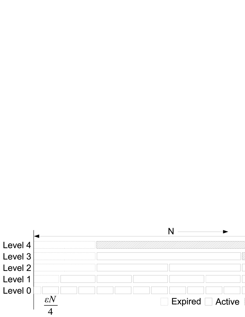
Figure 5: Levels and blocks in the fixed-size sliding window model.

Contrary to a fixed-size window, a variable-size window bears no limitation on insertion and deletion, so the window size keeps changing. Arasu et al. used $V(n,\epsilon)$ to denote a $epsilon$-approximate $Summary$ covering $n$ elements, where $n$ is the current size of the window. When a new element arrive, it becomes $V(n+1,\epsilon)$, and when the oldest element leaves, it gets $V(n-1,\epsilon)$. Besides, $F_{n}(N,\epsilon)$ is defined as a restriction of $F(N,\epsilon)$ to the last $n$ elements as Figure 6.

Figure 6: $F_{n}(N,\epsilon)$, a restriction of $F(N,\epsilon)$ to the last $n$ elements.

$F_{n}(N,\epsilon)$ is the same as $F(N,\epsilon)$ except that only blocks whose elements all belong to the most $n$ recent elements, instead of $N$ elements, are assumed active. $V(n,\epsilon)$ can be constructed by a set of $F_{n}(N,\epsilon)$ in the form of $\{F_{n}(2^{k},\frac{\epsilon}{2}),F_{n}(2^{k-1},\frac{\epsilon}{2}),...,F_{n}(\frac{2}{\epsilon},\frac{\epsilon}{2})\}$, where $k$ is an integer satisfying $2^{k-1}<n\leq 2^{k}$. $V(n,\epsilon)$ is maintained under various operations as follows:

• INSERT Update all $F_{n}(N,\epsilon)$ in $V(n,\epsilon)$ by incrementing $n$. If $n+1=2^{k}+1$, create $F_{2^{k}}(2^{k+1},\frac{\epsilon}{2})$ from $F_{2^{k}}(2^{k},\frac{\epsilon}{2})$ and insert the new element into it, thus getting $F_{2^{k}+1}(2^{k+1},\frac{\epsilon}{2})$.

• DELETE Compute $F_{n-1}(2^{k},\frac{\epsilon}{2})$ from $F_{n}(2^{k},\frac{\epsilon}{2})$. If $n-1=2^{k-1}$, remove $F_{2^{k-1}}(2^{k},\frac{\epsilon}{2})$.

• QUERY In order to query $\epsilon$-approximate quantiles over the most $n^{\prime}\leq n$ recent elements, find the integer $l$ satisfying $2^{l-1}<n\leq 2^{l}$. Then query $F_{n}(2^{l},\frac{\epsilon}{2})$ and return the answer.

The space complexity of the variable-size sliding window model is $O(\frac{1}{\epsilon}\log\frac{1}{\epsilon}\log(\epsilon{N})\log{N})$.

For uncertain data, one may still expect to obtain some consistent answers for queries [55]. Liang et al. [37] extended the problem and resolved approximate quantile queries over uncertain data streams. More specifically, it focuses on maintaining quantile $Summaries$ [34] over data streams whose elements are drawn from individually domain space, represented by continuous or discrete pdf. An uncertain data stream $S^{u}$ is a sequence of elements as $\{e_{1}^{u},e_{2}^{u},...\}$, each of which is drawn from a domain $D_{i}$ with pdf $f_{i}:D_{i}\rightarrow{(0,1]}$ such that $\sum_{p\in{D_{i}}}f_{i}(p)=1$. So, $S^{u}$ is a concise representation of exponential or infinite number of possible worlds $\mathbb{W}$. Each world $W=\{p_{i}|pi\in{D_{i}},i=1,2,...\}$ is a deterministic stream with probability $Pr(W)=\prod_{p_{i}\in{W}}f_{i}(p_{i})$. Therefore, the definition of approximate quantiles is generalized as the element $p\in{D_{i}}$ of $e_{i}^{u}\in{S^{u}}$ such that $\sum_{W\in\mathbb{W}}Pr(W)q(r,r_{W}^{p})-\sum_{W\in\mathbb{W}}Pr(W)q(r,r_{W}^{p_{min}})\leq\epsilon{N}$, where $r_{W}^{p}$ is the rank of $p$ in $W$ and $p_{min}$ is the element minimizing $\sum_{W\in\mathbb{W}}Pr(W)q(r,r_{W}^{p})$. Liang et al. proposed 2 error metric functions as $q(r,r_{W}^{p})$, the squared error function $q(r,r_{W}^{p})=(r-r_{W}^{p})^{2}$ and the related error function $q(r,r_{W}^{p})=r-r_{W}^{p}$. Following GK01, an online algorithm, namely UN-GK, is introduced. UN-GK adjusts tuples in $Summaries$ as $v_{i}=p_{i}\in{D_{j}}$ of $e_{j}^{u}\in{S^{u}}$, $g_{i}=PC_{min}(p_{i})-PC_{min}(p_{i-1})$, and $\Delta_{i}=PC_{max}(p_{i})-PC_{min}(p_{i})$, where $PC_{min}(p)$ and $PC_{max}(p)$ is the lower bound and the upper bound of probabilistic cardinality [56] of elements in $S^{u}$ no larger than $p$. And (2) is modified as $g_{i}+\Delta_{i}\leq 2\epsilon{PC(S^{u})}$, where $PC(S^{u})$ is the probabilistic cardinality of all elements in $S^{u}$ as $PC(S^{u})=|S^{u}|$. In this way, a $\epsilon$-approximate quantile can be queried anytime over an uncertain data stream, and its space complexity is $O(\frac{1}{\epsilon}\log(\epsilon{PC(S^{u})}))$.

II-B Distributed Model

In distributed models such as sensor networks, communication between nodes consumes much energy and cuts down the battery life of power-constrained devices. In addition, data transmission takes most of the running time of algorithms. Therefore, the priority of approximate quantile algorithms over distributed models is to reduce the communication cost by decreasing the size of transmitted data.

In 2004, Shrivastava et al. [20] designed an approximate quantile algorithm on distributed sensor networks with fixed-universe data, named as q-digest. Fixed-universe data refers to elements from a definite collection. Q-digest uses a unique binary tree structure to compress and store elements so that the storage space is cut down. The size of the fixed-universe collection is denoted as $\sigma$ and the compress coefficient is denoted as $k$. Figure 7 is the structure of a q-digest tree, which exists in each network node. Each node of the tree covers elements ranging from $v.min$ to $v.max$, recording the sum of their frequencies as $count(v)$. Each leaf represents one element in the universe, in other words, $v.min=v.max$. Take node $d$ as an example, its coverage is $[7,8]$ and there are 2 elements in this range. Besides, each node $v$ of the tree must satisfy:

$$count(v)\leq\lfloor\frac{n}{k}\rfloor$$ (6)

$$count(v)+count(v_{p})+count(v_{s})>\lfloor\frac{n}{k}\rfloor$$ (7)

where $v_{p}$ is $v$’s parent node and $v_{s}$ is its sibling node. (6) guarantees the upper bound of $v$’ coverage to narrow approximation error while (7) demonstrates when to merge two small nodes so that the storage cost can be reduced.

Figure 7: Structure of a q-digest tree, where $n=15,k=5,\sigma=8$.

Q-digest proposed an algorithm COMPRESS to merge nodes of a tree:

1. Scan nodes from bottom to top, from left to right, and sum up $count(v)$ and $count(v_{s})$ when (7) is violated.

2. Store the sum in $v_{p}$.

3. Remove the count in $v$ and $v_{s}$.

In order to reduce data communication, we number nodes in the tree from top to bottom, from left to right and only transmits nonempty nodes in the form of $(id(v),count(v))$, in which way every transmission contains only $O(\log{\sigma}+\log{N})$ data. For example, node $c$ in Figure 7 is transformed to $(6,2)$. When a network node receives q-digest trees from other nodes, it merges them with its own tree by adding up $count$ of nodes representing the same elements and applying COMPRESS. After merging all q-digest trees in the network, we can query quantiles by traversing the ultimate tree in postorder, summing up $count$ of passed nodes until the sum exceeds $\lfloor\phi{N}\rfloor$. The queried quantile is $v.max$ of the current node. The total communication cost of q-digest is $O(\frac{1}{\epsilon}|v|\log\sigma)$, where $|v|$ denotes the number of network nodes.

In the same year, Greenwald et al. [38] proposed an algorithm on distributed models, referred to as GK04. Unlike q-digest, GK04 does not require that all data be fixed-universe. It maintains a collection of $\frac{\epsilon}{2}$-approximate $Summaries$ [34], denoted as $S_{v}$, in each node $v$ in the sensor network. More specifically, $S_{v}=\{S^{1}_{v},S^{2}_{v},...,S^{k}_{v}\}$, where $S^{i}_{v}$ covers $n^{i}_{v}$ elements, and $S^{i}_{v}$ is classified as $class(S^{i}_{v})=\lfloor\log{n^{i}_{v}}\rfloor$. In the network, data are transmitted in the form of $S_{v}$. When data arrives at a node, it combines its own $S_{v}$ with the coming $S_{v}$ by iteratively merging $S_{v}$ of the same class from bottom to top. Once the iteration ends, a pruning algorithm is applied to $S^{i}_{v}$ to reduce the number of its tuples to $\log\frac{n_{v}}{\epsilon}+1$ at most. The pruning would bring up the approximation error of $S^{i}_{v}$ from $\epsilon^{\prime}$ to $\epsilon^{\prime}+\frac{\epsilon}{2\log{n_{v}}}$ at most, so a $\epsilon$-approximate $S$ is computed after merging $S_{v}$ from all nodes. GK04 only transmits $O(\frac{1}{\epsilon}\log^{2}{N})$ data, where $N$ is the number of all data in the network. Moreover, if the height of the network topology is far smaller than $N$, Greenwald et al. improved GK04 to reduce the total communication cost to $O(\frac{|v|}{\epsilon}\log{N}\log(\frac{h}{\epsilon}))$. Its basic idea is to apply a new operation, REDUCE, which makes sure that all nodes transmits less than $O(\log\frac{h}{\epsilon})$ $Summaries$, after merging and pruning.

Q-digest and GK04 are both offline algorithms that compute quantiles over stationary data in distributed models. Besides, there are also algorithms focusing on distributed models whose nodes receiving continuous data streams. In 2005, Cormode et al. [39] proposed a quantile algorithm for the scenario that multiple mutually isolated sensors are connected with one coordinator, which traces updating quantiles in real time. Its goal is to ensure $\epsilon$-approximate quantiles at the coordinator while minimizing communication cost between nodes and the coordinator. In general, each remote node maintains a local approximate $Summary$ [34] and informs the coordinator after certain number of updates. In the coordinator, the approximation error $\epsilon$ is divided into 2 parts as $\epsilon=\alpha+\beta$:

• $\alpha$ is the approximation error of local $Summaries$ sent to the coordinator.

• $\beta$ is the upper bound on the deviation of local $Summaries$ since the last communication.

Intuitively, larger $\beta$ allows for large deviation, thus less communication between nodes and the coordinator. But because $\epsilon$ is fixed, $\alpha$ is smaller, increasing the size of $Summaries$ sent to the coordinator each time. In other words, $\alpha$ and $\beta$ are on the trade-off relationship. To resolve the trade-off, Cormode et al. introduces a prediction model in each remote node that captures the anticipated behavior of its local data stream. With the model, the coordinator is able to predict the current state of a local data stream while computing the global $Summary$ and the remote node can check for the deviation between its $Summary$ and the coordinator’s prediction. The algorithm proposes 3 concise prediction models:

• Zero-Information Model assumes that there is no local update at any remote node since the last communication.

• Synchronous-Updates Model assumes that at each time step, each local node receives one update to its distribution.

• Update-Rates Model assumes that updates are observed at each local node at a uniform rate with a notion of global time.

Using prediction models to reduce communication times, the total communication cost of this algorithm is $O(\frac{|v|}{\epsilon^{2}}\log{N})$.

In 2013, Yi et al. [40] proposed an algorithm in the same scenario and optimized the cost to $O(\frac{|v|}{\epsilon}\log{N})$. The algorithm divides the whole tracking period into $O(\log{N})$ rounds. A new round begins whenever $N$ doubles. It first resolves the median-tracking problem, which can be easily generalized to the quantile-tracking problem. Assume that $M$ is the cardinality of data, fixed at the beginning of a round, and $m$ is the tracking median at the coordinator. The coordinator maintains 3 data structures. The first one is a dynamic set of disjoint intervals, each of which contains between $\frac{\epsilon{M}}{8}$ and $\frac{\epsilon{M}}{2}$ elements. The others are 2 counters $C.\Delta(L)$ and $C.\Delta(R)$, recording the number of elements received by all remote nodes to the left and the right of $m$ since last update respectively. They are guaranteed with an absolute error at most $\frac{\epsilon{M}}{8}$ by asking each remote node to send an update whenever it receives $\frac{\epsilon{M}}{8|v|}$ elements to the left or the right of $m$. When $|C.\Delta(L)-C.\Delta(R)|\geq\frac{\epsilon{M}}{2}$, $m$ is updated as follows:

1. Compute the total number of elements to the left and the right of $m$, $C.L$ and $C.R$ and let $d=\frac{1}{2}|C.L-C.R|$.

2. Compute the new median $m^{\prime}$ satisfying that $|r(m)-r(m^{\prime})-d|\leq\frac{\epsilon{M}}{4}$, where $r$ is the rank of element in all data. Replace $m$ with $m^{\prime}$. $m^{\prime}$ can be found quickly with the set of intervals. First find the first separating element $e_{1}$ of the intervals to the left of $M$. Then compute $n_{1}$, the number of elements at all remote sites that are in the interval $[e_{1},m]$. If $|n_{1}-d|\leq\frac{\epsilon{M}}{2}$, $e_{1}$ is $m^{\prime}$. Otherwise find the next separating element $e_{i}$ and count the number $n_{i}$ until $|n_{i}-d|\leq\frac{\epsilon{M}}{2}$, then set $m^{\prime}$ to $e_{i}$.

3. Set $C.\Delta(L)$ and $C.\Delta(R)$ to $0$.

Yi et al. has proved that $m$ is at most $\epsilon{M}$ elements away from the ground truth. Step 1 needs to exchange $O(|v|)$ messages. As for Step 2, $m^{\prime}$ can be found after at most $O(1)$ searches and the cost of each search is $O(|v|)$, making the total cost $O(|v|)$. Because each update increases $N$ by a factor of $1+\frac{\epsilon}{2}$, $m$ is updated at most $O(\frac{1}{\epsilon})$ times. So, the total communication cost is $O(\frac{|v|}{\epsilon})$ each round and $O(\frac{|v|}{\epsilon}\log{N})$ for the whole algorithm.

III Randomized Algorithms

Generally, randomized approximate quantile algorithms are combined with random sampling. They first sample a part of data and compute overall approximate quantiles with this portion. With less data taken into computation, the computation cost is cut down. In fact, many deterministic quantile algorithms propose randomized versions in this way [41, 36, 40].

III-A Streaming Model

Back to 1971, Vapnik et al. [57] proposed a randomized quantile algorithm with space complexity of $O(\frac{1}{\epsilon^{2}}\log\frac{1}{\epsilon})$. This benchmark were raised to $O(\frac{1}{\epsilon}\log^{2}\frac{1}{\epsilon})$ by Manku et al. [41] in 1999, referred to as MRL99. MRL99 does not require prior knowledge of the data size $N$ and occupies less space in experiments when $\phi$ is an extreme value. The algorithm are improved based on MRL98 [33] so they have the identical frame with only minor differences in the operation NEW:

1. For each buffer, randomly select an element among $r$ consecutive elements.

2. Repeats this operation $k$ times to get $k$ initial elements.

3. Set the buffer’s weight to $r$.

Notice that MRL99 equals with MRL98 if $r=1$. Because of the collapsing strategy as Figure 2, the larger weight a buffer has, the greater chance there its data must be retained while collapsing. If $r$ is kept consistent, the probability of newly arrived data being selected will go down continuously. So $r$ should keep changed dynamically, meaning the sampling is nonuniform. MRL99 initially sets $r$ to 2 and traces a parameter $h$, representing the maximum height of all buffers. When a buffer’s height reaches $h+i$ for the first time, where $i\geq 0$, $r$ is doubled. By tuning $h$, $b$ and $k$, MRL99 manages to compute approximate quantiles with a probability of at least $1-\delta$.

Recalling two sliding window models in Section II-A, Arasu et al. proposed the fact that the quantile of a random sample of size $O(\frac{1}{\epsilon^{2}}\log\delta^{-1})$ is an $\epsilon$-approximate quantile of $N$ elements with the probability at least $1-\delta$. To sample elements of specific size, a fast alternative is to randomly select one out of $2^{k}$ successive elements, where $k=\lfloor\log_{2}N/(\frac{1}{\epsilon^{2}}\log\delta^{-1})\rfloor$. In this way, $k$ grows logarithmically along with the data stream as required, so the approximation error and the randomization degree are guaranteed.

Another algorithm was proposed by Agarwal et al. [42], which is based on $Summaries$ [34]. Its basic idea is to sample tuples from multiple $Summaries$ and merge them to compute approximate quantiles with low space complexity. There are two situations while merging: same-weight merges and uneven-weight merges. Same-weight merges are for merging two $S$s covering the same number of elements. It contains following steps:

1. Combine the two $S$s in a sorted way.

2. Label the tuples in order and classify them by label parity.

3. Equiprobably select one class of tuples as the merged result $S_{merged}$.

Assuming each $S$ covers $k$ elements, if we have $k=O(\frac{1}{\epsilon}\sqrt{\log(\frac{1}{\epsilon\delta})})$, the algorithm will answer quantile queries with a probability of at least $1-\delta$. Uneven-weight merges are for merging two $S$s of different sizes, which can be reduced to same-weight merges by a so-called logarithmic technique [38]. The space complexity of the algorithm is $O(\frac{1}{\epsilon}\log^{1.5}\frac{1}{\epsilon})$.

However, Agarwal et al. just proposed and analyzed the algorithm in theory without implementation. Afterwards, Felber et al. [43] came up with a randomized algorithm whose space complexity is $O(\frac{1}{\epsilon}\log\frac{1}{\epsilon})$ but also did not realize it. Besides, this algorithm is not actually useful but only suitable for theoretical study because its hidden coefficient of $O$ is too large.

In 2016, Karnin et al. [44] achieved the space complexity of $O(\frac{1}{\epsilon}\log\log\frac{1}{\epsilon\delta})$. Its idea is based on MRL99 with some improvements. The first improvement is using increasing compactor capacities as the height gets larger (a compactor operates a COLLAPSE process in MRL99). The second comes from special handling of the top $\log\log\frac{1}{\delta}$ compactors. And the last is replacing those top compactors with $Summaries$ [34].

III-B Distributed Model

As for distributed models, Huang et al. [45] proposed a randomized quantile algorithm which brings down total communication cost from $O(|v|\log^{2}\frac{N}{\epsilon})$ in GK04 [38] to $O(\frac{1}{\epsilon}\sqrt{|v|h})$, where $h$ denotes the height of the network topology. It contains two version: the flat model and the tree model. For the flat model, all other nodes are assumed to be directly connected to the root node. The algorithm is designed as following steps:

1. Sample elements in node $v$ with a probability of $p$ and compute their ranks in $v$, denoted as $r(a,v)$ where $a$ is a sampled element.

2. Transmit sampled elements, as well as ones from its child nodes, to its parent node $v_{p}$.

3. Find predecessors of $a$, denoted as $pred(a,v_{s})$, in $v$’s sibling nodes $v_{s}$.

4. Estimate the rank of $a$ in $v_{s}$, denoted as $\hat{r}(a,v_{s})$, according to $r(pred(a,v_{s}),v_{s})$.

5. Compute the approximate rank of $a$ in $v_{p}$ as $r(a,v_{p})=\sum\hat{r}(a,v_{s})+r(a,v)$.

If elements are not uniformly distributed in the network and some nodes contain the majority, the total communication cost will increase dramatically as the effect of load imbalance. The algorithm resolves the problem by tuning $p$ based on data amount in each node:

• If the amount is greater than $N/\sqrt{|v|}$, $p$ is set to $1/(\epsilon{N_{v}})$.

• Otherwise, $p$ is set to $\Theta(\sqrt{|v|}/(\epsilon{N}))$.

The inconsistent probability of sampling makes sure that $O(\frac{1}{\epsilon})$ elements are sampled at most in each node no matter how many elements there exist at first. After transmitting all sampled elements to the root node, the element $a$ whose rank $r(a,v_{root})$ is closest to $\lfloor\phi{N}\rfloor$ is returned as the queried quantile. For the tree model, things become more complicated for two reasons. First, an intermediate node may suffer from heavy traffic going through if it has too many descendants without any data reduction. Second, each message needs $O(h)$ hops to reach the root node, leading to the total communication of $O(h\sqrt{|v|}/\epsilon)$. To resolve the first problem, Huang et al. proposed a algorithm MERGE in a systematic way to reduce data size. As for the second problem, the basic idea is to partition the routing tree into $t$ connected components, each of which has $O(|v|/t)$ nodes. Then each component is shrunk into a ”super node”. Now the height of the tree reduces to $t$. By setting $t=|v|/h$, the desired space bound becomes $O(\frac{1}{\epsilon}\sqrt{|v|h})$.

In 2018, Haeupler et al. [46], gave a drastically faster gossip algorithm, referred as Haeupler18, to compute approximate quantiles. Gossip algorithms [58] are algorithms that allow nodes in a distributed network to contact with each other randomly in each round and gradually converge to get final results. The algorithm contains two phases. In the first phase, each node adjusts its value so that the quantiles around $\phi$-quantile become the median quantiles approximately. And in the second phase, nodes compute their approximate median quantiles to get the global result. Haeupler et al. proved that the algorithm requires $O(\log\log{N}+\log\frac{1}{\epsilon})$ rounds to solve the $\epsilon$-approximate $\phi$-quantile problem with high probability.

IV Improvement

So far, in the discussion about approximate quantile algorithms, they are generally used with constant approximation error and indiscriminate performance on data regardless of data distribution. However, in some cases, we may have known that the data is skewed [59, 60, 61, 62, 63]. In other cases, quantile queries over high-speed data streams need to be updated and answered highly efficiently [64, 65]. In addition, there are also techniques for optimizing quantile computation with the help of GPUs [66, 67]. This section presents several techniques for improving the performance and efficiency of approximate quantile algorithms in various scenarios.

IV-A Skewness

The first algorithm is known as t-digest, proposed by Dunning et al. [63]. T-digest is for computing extreme quantiles such as the 99th, 99.9th and 99.99th percentiles. Totally different from q-digest, its basic idea is to cluster real-valued samples like histograms. But they differ in three aspects. First, the range covered by clusters may overlap. Second, instead of lower and upper bounds, a cluster is represented by a centroid value and an accumulated size on behalf of the number of elements. Third, clusters whose range is close to extreme values contain only a few elements so that the approximation error is not absolutely bounded, but relatively bounded, which is $\phi(1-\phi)$. T-digest can be applied to both streaming models and distributed models because the proposed cluster is a mergeable structure. The merge is restricted by the size bound of clusters. Dunning et al. proposed several scale functions to define the bound. The standard is that the size of each cluster should be small enough to get accurate quantiles, but large enough to avoid winding up too many clusters. A scale function is

$$f(\phi)=\frac{\delta}{2\pi}\sin^{-1}(2\phi-1)$$ (8)

where $\delta$ is the compression parameters and the size bound is defined as

$$W_{bound}=f(\frac{W_{left}+W}{N})-f(\frac{W_{left}}{N})\leq 1$$ (9)

where $W_{left}$ and $W$ are respectively the weight of clusters whose centroid values are smaller than that of the current cluster and of current cluster.

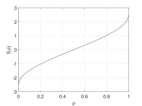
Figure 8: Function of (8) with $\delta=10$.

As Figure 8 shows, (8) is non-decreasing and is steeper when $\phi$ is closer to $0$ or $1$, which means clusters covering extreme values have smaller size, making the algorithm more accurate for computing extreme quantiles and more robust for skewed data.

The second algorithm, proposed by Lin et al. [61] and elaborated by Liu et al. [62], is aimed at streaming models, using nonlinear interpolation. The algorithm maintains two buffers, the quantile buffer $Q=\{q_{1},q_{2},...,q_{m}\}$, where $q_{i}$ is the approximate $\phi_{i}$-quantile, and the data buffer $B$ of size $n$, holding the most recent $n$ elements. $Q$ is estimated from observed data and incrementally updated when $B$ is full-filled. In order to estimate the extreme quantiles accurately, the nonlinear interpolation $F(x)$, which is an approximate distribution function estimated from a training set stream, is leveraged together with $B$ and $Q$ to update $Q$.

The third algorithm was proposed by Cormode et al. [59] for skewed data. Again, the algorithm is an improved version of GK01 for two problems. The first problem is the biased quantiles problem. Low-biased quantiles are the set of elements whose rank $\lfloor\phi^{i}N\rfloor$ for $i=1,2,...,\log_{1/\phi}N$, and high-biased quantiles are symmetry by reversing the ordering relation. The definition is easy to be generalized to approximate quantiles. The problem is computing the first $k$ elements in high-biased approximate quantiles. Similar with GK01 that $g_{i}$ and $\Delta_{i}$ are restricted by $g_{i}+\Delta_{i}\leq\lfloor 2\epsilon{N}\rfloor$, the algorithm generalizes the restriction as $g_{i}+\Delta_{i}\leq f(r_{i},N)$, where $f(r_{i},N)$ is an appropriate function. $r_{i}$ is the rank of $v_{i}$ equaling $\sum_{j=1}^{i-1}g_{j}$. For the biased quantiles problem, $f(r_{i},N)$ is set to $2\epsilon{r_{i}}$. The restriction is tighter than that in GK01 so the correctness is guaranteed. Cormode et al. proved that the space lower bound is $\Omega(\frac{1}{\epsilon}min(k\log\frac{1}{\phi},\log(\epsilon{N})))$. The other problem is targeted quantiles problem that quantiles meeting a set of pairs $T=\{(\phi_{i},\epsilon_{i})\}$ are required to be maintained. In such case, $f(r_{i},N)$ is set to $\frac{2\epsilon_{i}r_{i}}{\phi_{i}}$ if $\phi_{i}N\leq r_{i}\leq N$ and $\frac{2\epsilon_{i}(N-r_{i})}{1-\phi_{i}}$ if $0\leq r_{i}\leq\phi_{i}N$. Also, the state-of-the-art space upper bound for biased quantile computation is $O(\frac{1}{\epsilon}\log^{3}{\epsilon{N}})$ with a deterministic comparison-based merging-and-pruning strategy [68]. As for a randomized version, Zhang et al. [69] achieved expected space of $O(\frac{1}{\epsilon}\log(\frac{1}{\epsilon}\log\frac{1}{\epsilon})\frac{\log^{2+\alpha}{\epsilon{N}}}{1-2^{-\alpha}})$ where $\alpha>0$ and worst case of $O(\frac{1}{\epsilon^{2}}\log\frac{1}{\epsilon}\log^{2}{\epsilon{N}})$.

For problems resolved by q-digest [20] that all elements are selected from a fixed-universe collection, Cormode et al. [60] combined the binary tree structure in q-digest and standard dictionary data structures [70], proposing a new deterministic algorithm to compute biased quantiles with space complexity of $O(\frac{1}{\epsilon}\log{\sigma}\log(\epsilon{N}))$, where $\sigma$ denotes the size of the fixed-universe collection. And a simpler sampling-based approach by Gupta et al. [71] uses space of $O(\epsilon^{-3}\log^{2}N\log\sigma)$.

IV-B High-Speed Data Streams

In order to compute quantiles over high-speed data streams, both computational cost and per-element update cost need to be low. Zhang et al. [65] proposed an algorithm for both fixed- and arbitrary- size high-speed data streams. Let $N$ and $n$ denote the number of elements in the entire data stream and elements seen so far. For the fixed-size data streams, where $N$ is given, a multi-level summary structure $S=\{s_{0},s_{1},...,s_{L}\}$ is maintained, where $s_{i}$ is the summary at level $i$, as shown in Figure 9. Each element in $s$ is stored with its upper and lower bound of rank, $r_{min}(e)$ and $r_{max}(e)$.

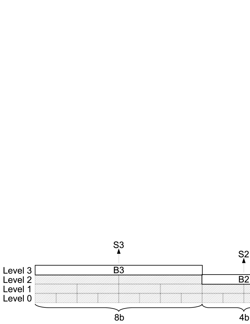
Figure 9: A multi-level summary structure with $L=3$.

The data stream is divided into blocks of size $b=\lfloor\frac{1}{\epsilon}\log\epsilon{N}\rfloor$ and $s_{i}$ covers a disjoint bag $B_{i}$. Among bags, $B_{0}$ contains the most recent blocks even though it may be incomplete. The structure is maintained as follows:

1. Insert the new element to $s_{0}$.

2. If $|s_{0}|<b$, the procedure is done. Otherwise, compress $s_{0}$ to generate a sketch $s_{c}$ of size $\lfloor\frac{b}{2}\rfloor$ and send it to level $1$. COMPRESS would raise the approximation error from $\epsilon_{0}$ to $\epsilon_{0}+\frac{1}{b}$.

3. If $s_{1}$ is empty, set $s_{1}$ to $s_{c}$ and the procedure is done. Otherwise, merge $s_{1}$ with $s_{c}$ and empty $s_{0}$. Finally, compress the merged $s$ and send it to level $2$.

4. Repeat the steps above until an empty $s_{i}$ is found.

To answer quantiles, the algorithm first sorts $s_{0}$ and merges $s$ at all levels. Then it searches the merged $s$ and return the element satisfying that $r_{min}(e)\geq r-\lfloor\epsilon{N}\rfloor$ and $r_{max}(e)\leq r+\lfloor\epsilon{N}\rfloor$. As for the arbitrary-size data streams, the basic idea is to partition the data stream into disjoint sub-streams $d_{i}$ with the size $\frac{2^{i}}{\epsilon}$ in their arrival order, and use the algorithm for the fixed-size data streams on each sub-stream because their length is known now. The computational cost and the per-element update cost of both algorithms are $O(N\log(\frac{1}{\epsilon}\log\epsilon{N}))$ and $O(\log\log{N})$. Compared to GK01, the experimental results over high-speed data streams are reported to achieve about $200\sim 300x$ speedup.

Besides, in order to lighten the burden of massive continuous quantile queries with different $\phi$ and $\epsilon$, Lin et al. [64] proposed 2 techniques for processing queries. The first technique is to cluster multiple queries as a single query virtually while guaranteeing accuracy. Its basic idea is to cluster the queries that share some common results. The second technique is to minimize both the total number of times for reprocessing and the number of clusters. It adopts a trigger-based lazy update paradigm.

IV-C GPU

Govindaraju et al. [66] studied optimizing quantile computation using graphics processors, or GPU for short. GPUs are well designed for rendering and allow many rendering applications to raise memory performance [72]. In order to utilize the high computational power of GPUs, Govindaraju et al. proposed an algorithm based on sorting networks. Sorting networks are a set of sorting algorithms mapped well to mesh-based architectures [73]. Operations in the algorithm, including comparisons and comparator mapping, are realized by color blending and texture mapping in GPUs. The theoretical algorithm they used is GK04 [38] and by taking advantage of high computational power and memory bandwidth of GPUs, the algorithm offers great performance for quantile computation over streaming models.

V Approximate Quantile Computation Tools

Over the past decades, many off-the-shelf, open-source packages or tools for quantile computation have been developed and available to users. Some of them are based on exact quantile computation while others implement approximate quantile computation. In this section, we review such tools, focusing on their algorithmic theories and application scenarios.

Most basically, SQL provides a window function $ntile$ which helps with quantile computation. It receives a parameter $b$ and partitions a set of data into $b$ buckets equally. Therefore, with $sortBy$ and $ntile$, we can partition the data in order and get the leading element of each partition as the quantile. Also, these quantiles are exact.

MATLAB is a famous numerical computing environment and programming language. It provides comprehensive packages for computing various statistics or functions. Quantiles are included as its in-tool function. The function $quantile$ receives a few parameters, including a numerical array, the cumulative probability and the computation kind. It computes quantiles in either exact or approximate way. It computes exact quantiles by the classic algorithm that uses sort. And it implements t-digest [63] for approximate quantiles. So, this function is suitable to compute quantiles over distributed models, which benefit from parallel computation.

The distributed cluster-computing framework, Spark, provides approximate quantile computation since version 2.0. It implements GK01 and can be called in many programming languages such as Python, Scala, R and Java. Computing on a Spark dataframe, the function contains 3 parameters as a dataframe, the name of a numerical column, a list of quantile probabilities and the approximation error. Since version 2.2, the function has been upgraded to support computation over multiple dataframe columns.

In Java, Google publishes an open-source set of core libraries, named as Guava. It includes new collection types, graph libraries, support for concurrency, etc. Also, quantile computation is included in its functions as $median()$ and $percentiles()$. The quantiles are exact results so the average time complexity of its implementation is $O(n)$ while the worst case time complexity is $O(N^{2})$. It optimizes multiple quantile computation on the same dataset with indexes, improving the performance in some degree. Another package that supports quantile computation is Apache Beam. It is a unified programming model for batch and streaming data processing on execution engines. Unlike Guava, it implements approximate quantile computation.

The programming language, Rust, implements approximate quantile computation over data streams with a moderate amount of memory. It implements the algorithms, GK01 [34] and CKMS [59], so that no boatload of information is stored in memory. Besides, it implements a variant of quantile computation, an $\epsilon$-approximate frequency count for a stream, outputting the $k$ most frequent elements, with the algorithm Misra-Gries [74], which helps with an estimation of quantiles as well. As for C++, a peer-reviewed set of core libraries, Boost, provides exact quantile computation as its in-tool function.

VI Future Directions and Conclusions

In this survey, we have presented a comprehensive survey of approximate quantile computation. Readers who want to know more about the performance of basic quantile algorithms can read a paper by Luo et al. [29], which implements a part of the quantile algorithms above and compares them by experiments. Besides, Cormode et al. [75] summarized lower bounds of the researches about comparison-based quantile computation so far and proved that the space complexity of GK01 is optimal by showing a matching lower bound.

Even though approximate quantiles have been studied for more than three decades, there is still plenty of room for improvement. The explosion of data also brings new challenges to this field. There are many studies to resolve quantile computation in large-scale data, but not enough. Besides, with the development of industries, new scenarios keep appearing so that quantile computation should be optimized specifically as well. And the evolvement of techniques brings new direction and new potential to quantile computation. Here we present a few future directions for quantile computation.

First, almost all quantile algorithms require at least one-pass scan over the entire dataset, no matter it is applied on streaming models or distributed models. However, at some time, the cost of scanning the entire data is intolerable if quantile queries are demanded to be answered in time. In such case, only a portion of the entire dataset is permitted into the process of the whole algorithm. This condition is more restricted than that in existing randomized quantile algorithms. Even if randomized algorithms sample a part of data to save the space of computation, the process of sampling requires the participation of the entire dataset, which means that they need to scan all data once. To resolve the problem, we need to determine the sampling methods first. Unlike fine-grained sampling in existing randomized algorithms, we may use coarse-grained sampling, such as sampling in the unit of block. The method should also take the way of storage into account. For example, if the dataset is stored in distributed HDFS [76], we may sample part of blocks, avoiding scanning the entire data. The sampling methods may be exclusive, varying based on applications. After determining sampling methods, we need to consider how much data is sampled to balance the accuracy and the occupation of time and space. One direction is to simulate the idea in machine learning [77] that data are trained (or sampled in our situation) continuously until the quantile result converges.

Second, many new computation engines are being developed. They can be classified into two categories in general. One is streaming computation engines and the other is distributed computation engines. Streaming computation engines, represented by Spark Streaming, Storm and Flink [78], are aimed at real-time streaming needs with minor difference in some ways. For example, Storm and Flink behave like true streaming processing systems with lower latencies while Spark Streaming can handle higher throughput at the cost of higher latencies. Distributed computation engines, represented by Spark and GraphLab [79], are designed to analyze distributed data such as datasets with graph properties.They have their pros and cons in heterogeneous scenarios as well. The characteristics of these engines may be utilized in the implementation of algorithms. As reviewed in Section V, only a small fraction of approximate quantile algorithms is implemented in them such as GK01 in Spark. But many other algorithms are still needed to be implemented and optimized purposefully. For example, Spark [80] is a framework for computation in distributed clusters, supporting parallel computation naturally and having potential of benefitting many quantile algorithms such as MRL98. Its streaming version, Spark Structured Streaming [81], supports stream processing, as well as window operations. It may help quantile algorithms over streaming models, such as Lin SW and Lin n-of-N [35], to be implemented in a more efficient way, even though the theoretical complexity remains the same. Many quantile algorithms are implemented with basic languages while others are even without implementation. Transplanting them to new computation engines is not an easy work and there is great room for optimization.

Third, with the appearance of new specific application scenarios, the requirements of approximate quantile algorithms evolve as well. For example, nowadays, more and more attention is being paid to the correlation of data, and data graph is one way to present the correlation. In a data graph, each edge is usually associated with a weight, representing frequencies of the appearance of the correlation. One may need to determine a threshold for pruning edges by their weights for better performance in analysis [82, 83]. And we can use quantiles to determine the threshold. However, unlike random sampling in a dataset, the edges in a graph are correlated (the frequencies of two edges connecting to the same vertex are correlated). Maybe it is a challenge, as well as an opportunity, to efficiently compute approximate quantiles in a correlated data graph. Furthermore, if the graph is constrained by some patterns [84, 85], the algorithms may be improved and optimized correspondingly. Other cases include computing quantiles in the Blockchain network [86]. Unlike traditional distributed models, which have a master node and multiple slave nodes, the Blockchain network is decentralized, making merging quantile algorithms infeasible. Further research is needed for computing approximate quantiles in such network. Haeupler et al. [46], which uses gossip algorithms, provides a good direction, but there is much more to be done.

References

- [1] Z. Abedjan, L. Golab, and F. Naumann, “Profiling relational data: a survey,” VLDB J., vol. 24, no. 4, pp. 557–581, 2015.
- [2] S. Song, L. Chen, and P. S. Yu, “Comparable dependencies over heterogeneous data,” VLDB J., vol. 22, no. 2, pp. 253–274, 2013.
- [3] Z. He, Z. Cai, S. Cheng, and X. Wang, “Approximate aggregation for tracking quantiles and range countings in wireless sensor networks,” Theor. Comput. Sci., vol. 607, pp. 381–390, 2015.
- [4] S. Song, H. Zhu, and L. Chen, “Probabilistic correlation-based similarity measure on text records,” Inf. Sci., vol. 289, pp. 8–24, 2014.
- [5] Y. Wang, S. Song, L. Chen, J. X. Yu, and H. Cheng, “Discovering conditional matching rules,” TKDD, vol. 11, no. 4, pp. 46:1–46:38, 2017.
- [6] A. Zhang, S. Song, J. Wang, and P. S. Yu, “Time series data cleaning: From anomaly detection to anomaly repairing,” PVLDB, vol. 10, no. 10, pp. 1046–1057, 2017.
- [7] S. Song, L. Chen, and H. Cheng, “Efficient determination of distance thresholds for differential dependencies,” IEEE Trans. Knowl. Data Eng., vol. 26, no. 9, pp. 2179–2192, 2014.
- [8] S. Song and L. Chen, “Differential dependencies: Reasoning and discovery,” ACM Trans. Database Syst., vol. 36, no. 3, pp. 16:1–16:41, 2011.
- [9] S. Song, A. Zhang, J. Wang, and P. S. Yu, “SCREEN: stream data cleaning under speed constraints,” in Proceedings of the 2015 ACM SIGMOD International Conference on Management of Data, Melbourne, Victoria, Australia, May 31 - June 4, 2015, pp. 827–841, 2015.
- [10] A. Zhang, S. Song, and J. Wang, “Sequential data cleaning: A statistical approach,” in Proceedings of the 2016 International Conference on Management of Data, SIGMOD Conference 2016, San Francisco, CA, USA, June 26 - July 01, 2016 (F. Özcan, G. Koutrika, and S. Madden, eds.), pp. 909–924, ACM, 2016.
- [11] S. Song, C. Li, and X. Zhang, “Turn waste into wealth: On simultaneous clustering and cleaning over dirty data,” in Proceedings of the 21th ACM SIGKDD International Conference on Knowledge Discovery and Data Mining, Sydney, NSW, Australia, August 10-13, 2015, pp. 1115–1124, 2015.
- [12] S. Guha and A. McGregor, “Stream order and order statistics: Quantile estimation in random-order streams,” SIAM J. Comput., vol. 38, no. 5, pp. 2044–2059, 2009.
- [13] B. Babcock, S. Babu, M. Datar, R. Motwani, and J. Widom, “Models and issues in data stream systems,” in Proceedings of the Twenty-first ACM SIGACT-SIGMOD-SIGART Symposium on Principles of Database Systems, June 3-5, Madison, Wisconsin, USA, pp. 1–16, 2002.
- [14] S. Muthukrishnan, “Data streams: Algorithms and applications,” Foundations and Trends in Theoretical Computer Science, vol. 1, no. 2, 2005.
- [15] A. Segall, “Distributed network protocols,” IEEE Trans. Information Theory, vol. 29, no. 1, pp. 23–34, 1983.
- [16] Y. Sun, S. Song, C. Wang, and J. Wang, “Swapping repair for misplaced attribute values,” in 36st International Conference on Data Engineering (ICDE’20), IEEE, 2020.
- [17] F. Gao, S. Song, L. Chen, and J. Wang, “Efficient set-correlation operator inside databases,” J. Comput. Sci. Technol., vol. 31, no. 4, pp. 683–701, 2016.
- [18] R. Pike, S. Dorward, R. Griesemer, and S. Quinlan, “Interpreting the data: Parallel analysis with sawzall,” Scientific Programming, vol. 13, no. 4, pp. 277–298, 2005.
- [19] G. Cormode, T. Johnson, F. Korn, S. Muthukrishnan, O. Spatscheck, and D. Srivastava, “Holistic udafs at streaming speeds,” in Proceedings of the ACM SIGMOD International Conference on Management of Data, Paris, France, June 13-18, 2004, pp. 35–46, 2004.
- [20] N. Shrivastava, C. Buragohain, D. Agrawal, and S. Suri, “Medians and beyond: new aggregation techniques for sensor networks,” in Proceedings of the 2nd International Conference on Embedded Networked Sensor Systems, SenSys 2004, Baltimore, MD, USA, November 3-5, 2004, pp. 239–249, 2004.
- [21] C. Leys, C. Ley, O. Klein, P. Bernard, and L. Licata, “Detecting outliers: Do not use standard deviation around the mean, use absolute deviation around the median,” Journal of Experimental Social Psychology, vol. 49, no. 4, pp. 764–766, 2013.
- [22] S. Song, Y. Cao, and J. Wang, “Cleaning timestamps with temporal constraints,” PVLDB, vol. 9, no. 10, pp. 708–719, 2016.
- [23] M. B. Greenwald and S. Khanna, “Quantiles and equi-depth histograms over streams,” in Data Stream Management - Processing High-Speed Data Streams, pp. 45–86, 2016.
- [24] P. Indyk, “Algorithms for dynamic geometric problems over data streams,” in Proceedings of the 36th Annual ACM Symposium on Theory of Computing, Chicago, IL, USA, June 13-16, 2004, pp. 373–380, 2004.
- [25] M. Blum, R. W. Floyd, V. R. Pratt, R. L. Rivest, and R. E. Tarjan, “Time bounds for selection,” J. Comput. Syst. Sci., vol. 7, no. 4, pp. 448–461, 1973.
- [26] J. I. Munro and M. Paterson, “Selection and sorting with limited storage,” Theor. Comput. Sci., vol. 12, pp. 315–323, 1980.
- [27] J. Wang, S. Song, X. Zhu, X. Lin, and J. Sun, “Efficient recovery of missing events,” IEEE Trans. Knowl. Data Eng., vol. 28, no. 11, pp. 2943–2957, 2016.
- [28] S. Mittal, “A survey of techniques for approximate computing,” ACM Comput. Surv., vol. 48, no. 4, pp. 62:1–62:33, 2016.
- [29] G. Luo, L. Wang, K. Yi, and G. Cormode, “Quantiles over data streams: experimental comparisons, new analyses, and further improvements,” VLDB J., vol. 25, no. 4, pp. 449–472, 2016.
- [30] S. Ganguly and A. Majumder, “Cr-precis: A deterministic summary structure for update data streams,” in Combinatorics, Algorithms, Probabilistic and Experimental Methodologies, First International Symposium, ESCAPE 2007, Hangzhou, China, April 7-9, 2007, Revised Selected Papers, pp. 48–59, 2007.
- [31] A. Deshpande, C. Guestrin, S. Madden, J. M. Hellerstein, and W. Hong, “Model-driven data acquisition in sensor networks,” in (e)Proceedings of the Thirtieth International Conference on Very Large Data Bases, VLDB 2004, Toronto, Canada, August 31 - September 3 2004, pp. 588–599, 2004.
- [32] R. Motwani and P. Raghavan, “Randomized algorithms,” ACM Comput. Surv., vol. 28, no. 1, pp. 33–37, 1996.
- [33] G. S. Manku, S. Rajagopalan, and B. G. Lindsay, “Approximate medians and other quantiles in one pass and with limited memory,” in SIGMOD 1998, Proceedings ACM SIGMOD International Conference on Management of Data, June 2-4, 1998, Seattle, Washington, USA, pp. 426–435, 1998.
- [34] M. Greenwald and S. Khanna, “Space-efficient online computation of quantile summaries,” in Proceedings of the 2001 ACM SIGMOD international conference on Management of data, Santa Barbara, CA, USA, May 21-24, 2001, pp. 58–66, 2001.
- [35] X. Lin, H. Lu, J. Xu, and J. X. Yu, “Continuously maintaining quantile summaries of the most recent N elements over a data stream,” in Proceedings of the 20th International Conference on Data Engineering, ICDE 2004, 30 March - 2 April 2004, Boston, MA, USA, pp. 362–373, 2004.
- [36] A. Arasu and G. S. Manku, “Approximate counts and quantiles over sliding windows,” in Proceedings of the Twenty-third ACM SIGACT-SIGMOD-SIGART Symposium on Principles of Database Systems, June 14-16, 2004, Paris, France, pp. 286–296, 2004.
- [37] C. Liang, M. Li, and B. Liu, “Online computing quantile summaries over uncertain data streams,” IEEE Access, vol. 7, pp. 10916–10926, 2019.
- [38] M. Greenwald and S. Khanna, “Power-conserving computation of order-statistics over sensor networks,” in Proceedings of the Twenty-third ACM SIGACT-SIGMOD-SIGART Symposium on Principles of Database Systems, June 14-16, 2004, Paris, France, pp. 275–285, 2004.
- [39] G. Cormode, M. N. Garofalakis, S. Muthukrishnan, and R. Rastogi, “Holistic aggregates in a networked world: Distributed tracking of approximate quantiles,” in Proceedings of the ACM SIGMOD International Conference on Management of Data, Baltimore, Maryland, USA, June 14-16, 2005, pp. 25–36, 2005.
- [40] K. Yi and Q. Zhang, “Optimal tracking of distributed heavy hitters and quantiles,” Algorithmica, vol. 65, no. 1, pp. 206–223, 2013.
- [41] G. S. Manku, S. Rajagopalan, and B. G. Lindsay, “Random sampling techniques for space efficient online computation of order statistics of large datasets,” in SIGMOD 1999, Proceedings ACM SIGMOD International Conference on Management of Data, June 1-3, 1999, Philadelphia, Pennsylvania, USA, pp. 251–262, 1999.
- [42] P. K. Agarwal, G. Cormode, Z. Huang, J. M. Phillips, Z. Wei, and K. Yi, “Mergeable summaries,” ACM Trans. Database Syst., vol. 38, no. 4, pp. 26:1–26:28, 2013.
- [43] D. Felber and R. Ostrovsky, “A randomized online quantile summary in o(1/epsilon * log(1/epsilon)) words,” in Approximation, Randomization, and Combinatorial Optimization. Algorithms and Techniques, APPROX/RANDOM 2015, August 24-26, 2015, Princeton, NJ, USA, pp. 775–785, 2015.
- [44] Z. S. Karnin, K. J. Lang, and E. Liberty, “Optimal quantile approximation in streams,” in IEEE 57th Annual Symposium on Foundations of Computer Science, FOCS 2016, 9-11 October 2016, Hyatt Regency, New Brunswick, New Jersey, USA, pp. 71–78, 2016.
- [45] Z. Huang, L. Wang, K. Yi, and Y. Liu, “Sampling based algorithms for quantile computation in sensor networks,” in Proceedings of the ACM SIGMOD International Conference on Management of Data, SIGMOD 2011, Athens, Greece, June 12-16, 2011, pp. 745–756, 2011.
- [46] B. Haeupler, J. Mohapatra, and H. Su, “Optimal gossip algorithms for exact and approximate quantile computations,” in Proceedings of the 2018 ACM Symposium on Principles of Distributed Computing, PODC 2018, Egham, United Kingdom, July 23-27, 2018, pp. 179–188, 2018.
- [47] K. Alsabti, S. Ranka, and V. Singh, “A one-pass algorithm for accurately estimating quantiles for disk-resident data,” in VLDB’97, Proceedings of 23rd International Conference on Very Large Data Bases, August 25-29, 1997, Athens, Greece, pp. 346–355, 1997.
- [48] F. Chen, D. Lambert, and J. C. Pinheiro, “Incremental quantile estimation for massive tracking,” in Proceedings of the sixth ACM SIGKDD international conference on Knowledge discovery and data mining, Boston, MA, USA, August 20-23, 2000, pp. 516–522, 2000.
- [49] R. Y. S. Hung and H. Ting, “An w(\frac1e log\frac1e)\omega(\frac{1}{\varepsilon} \log \frac{1}{\varepsilon}) space lower bound for finding epsilon-approximate quantiles in a data stream,” in Frontiers in Algorithmics, 4th International Workshop, FAW 2010, Wuhan, China, August 11-13, 2010. Proceedings, pp. 89–100, 2010.
- [50] R. Jain and I. Chlamtac, “The p2 algorithm for dynamic calculation of quantiiles and histograms without storing observations,” Commun. ACM, vol. 28, no. 10, pp. 1076–1085, 1985.
- [51] R. Agrawal and A. N. Swami, “A one-pass space-efficient algorithm for finding quantiles,” in Advances in Data Management, Proceedings of the 7th International Conference on Management of Data, COMAD 1995, December 28-30, 1995, Pune, India, 1995.
- [52] A. Lall, “Data streaming algorithms for the kolmogorov-smirnov test,” in 2015 IEEE International Conference on Big Data, Big Data 2015, Santa Clara, CA, USA, October 29 - November 1, 2015, pp. 95–104, 2015.
- [53] Y. Tao, W. Lin, and X. Xiao, “Minimal mapreduce algorithms,” in Proceedings of the ACM SIGMOD International Conference on Management of Data, SIGMOD 2013, New York, NY, USA, June 22-27, 2013, pp. 529–540, 2013.
- [54] M. Datar, A. Gionis, P. Indyk, and R. Motwani, “Maintaining stream statistics over sliding windows,” SIAM J. Comput., vol. 31, no. 6, pp. 1794–1813, 2002.
- [55] X. Lian, L. Chen, and S. Song, “Consistent query answers in inconsistent probabilistic databases,” in Proceedings of the ACM SIGMOD International Conference on Management of Data, SIGMOD 2010, Indianapolis, Indiana, USA, June 6-10, 2010 (A. K. Elmagarmid and D. Agrawal, eds.), pp. 303–314, ACM, 2010.
- [56] C. Liang, Y. Zhang, P. Shi, and Z. Hu, “Learning accurate very fast decision trees from uncertain data streams,” Int. J. Systems Science, vol. 46, no. 16, pp. 3032–3050, 2015.
- [57] V. N. Vapnik and A. Y. Chervonenkis, “On the uniform convergence of relative frequencies of events to their probabilities,” in Measures of complexity, pp. 11–30, Springer, 2015.
- [58] S. P. Boyd, A. Ghosh, B. Prabhakar, and D. Shah, “Gossip algorithms: design, analysis and applications,” in INFOCOM 2005. 24th Annual Joint Conference of the IEEE Computer and Communications Societies, 13-17 March 2005, Miami, FL, USA, pp. 1653–1664, 2005.
- [59] G. Cormode, F. Korn, S. Muthukrishnan, and D. Srivastava, “Effective computation of biased quantiles over data streams,” in Proceedings of the 21st International Conference on Data Engineering, ICDE 2005, 5-8 April 2005, Tokyo, Japan, pp. 20–31, 2005.
- [60] G. Cormode, F. Korn, S. Muthukrishnan, and D. Srivastava, “Space- and time-efficient deterministic algorithms for biased quantiles over data streams,” in Proceedings of the Twenty-Fifth ACM SIGACT-SIGMOD-SIGART Symposium on Principles of Database Systems, June 26-28, 2006, Chicago, Illinois, USA, pp. 263–272, 2006.
- [61] Z. Lin, J. Liu, and N. Lin, “Accurate quantile estimation for skewed data streams,” in 28th IEEE Annual International Symposium on Personal, Indoor, and Mobile Radio Communications, PIMRC 2017, Montreal, QC, Canada, October 8-13, 2017, pp. 1–7, 2017.
- [62] J. Liu, W. Zheng, Z. Lin, and N. Lin, “Accurate quantile estimation for skewed data streams using nonlinear interpolation,” IEEE Access, vol. 6, pp. 28438–28446, 2018.
- [63] T. Dunning and O. Ertl, “Computing extremely accurate quantiles using t-digests,” CoRR, vol. abs/1902.04023, 2019.
- [64] X. Lin, J. Xu, Q. Zhang, H. Lu, J. X. Yu, X. Zhou, and Y. Yuan, “Approximate processing of massive continuous quantile queries over high-speed data streams,” IEEE Trans. Knowl. Data Eng., vol. 18, no. 5, pp. 683–698, 2006.
- [65] Q. Zhang and W. Wang, “A fast algorithm for approximate quantiles in high speed data streams,” in 19th International Conference on Scientific and Statistical Database Management, SSDBM 2007, 9-11 July 2007, Banff, Canada, Proceedings, p. 29, 2007.
- [66] N. K. Govindaraju, N. Raghuvanshi, and D. Manocha, “Fast and approximate stream mining of quantiles and frequencies using graphics processors,” in Proceedings of the ACM SIGMOD International Conference on Management of Data, Baltimore, Maryland, USA, June 14-16, 2005, pp. 611–622, 2005.
- [67] Y. ZHOU, H. WANG, and C.-t. CHENG, “Parallel computing method of data stream quantiles with gpu,” Journal of Computer Applications, vol. 2, 2010.
- [68] Q. Zhang and W. Wang, “An efficient algorithm for approximate biased quantile computation in data streams,” in Proceedings of the Sixteenth ACM Conference on Information and Knowledge Management, CIKM 2007, Lisbon, Portugal, November 6-10, 2007, pp. 1023–1026, 2007.
- [69] Y. Zhang, X. Lin, J. Xu, F. Korn, and W. Wang, “Space-efficient relative error order sketch over data streams,” in Proceedings of the 22nd International Conference on Data Engineering, ICDE 2006, 3-8 April 2006, Atlanta, GA, USA, p. 51, 2006.
- [70] T. H. Cormen, C. E. Leiserson, and R. L. Rivest, Introduction to Algorithms. The MIT Press and McGraw-Hill Book Company, 1989.
- [71] A. Gupta and F. Zane, “Counting inversions in lists,” in Proceedings of the Fourteenth Annual ACM-SIAM Symposium on Discrete Algorithms, January 12-14, 2003, Baltimore, Maryland, USA, pp. 253–254, 2003.
- [72] O. Rubinstein, D. Reed, and J. Alben, “Gpu rendering to system memory,” Oct. 27 2005. US Patent App. 10/833,694.
- [73] K. E. Batcher, “Sorting networks and their applications,” in American Federation of Information Processing Societies: AFIPS Conference Proceedings: 1968 Spring Joint Computer Conference, Atlantic City, NJ, USA, 30 April - 2 May 1968, pp. 307–314, 1968.
- [74] J. Misra and D. Gries, “Finding repeated elements,” Sci. Comput. Program., vol. 2, no. 2, pp. 143–152, 1982.
- [75] G. Cormode and P. Veselý, “Tight lower bound for comparison-based quantile summaries,” CoRR, vol. abs/1905.03838, 2019.
- [76] D. Borthakur et al., “Hdfs architecture guide,” Hadoop Apache Project, vol. 53, no. 1-13, p. 2, 2008.
- [77] C. M. Bishop and N. M. Nasrabadi, “Pattern Recognition and Machine Learning,” J. Electronic Imaging, vol. 16, no. 4, p. 049901, 2007.
- [78] S. Chintapalli, D. Dagit, B. Evans, R. Farivar, T. Graves, M. Holderbaugh, Z. Liu, K. Nusbaum, K. Patil, B. Peng, and P. Poulosky, “Benchmarking streaming computation engines: Storm, flink and spark streaming,” in 2016 IEEE International Parallel and Distributed Processing Symposium Workshops, IPDPS Workshops 2016, Chicago, IL, USA, May 23-27, 2016, pp. 1789–1792, 2016.
- [79] J. Wei, K. Chen, Y. Zhou, Q. Zhou, and J. He, “Benchmarking of distributed computing engines spark and graphlab for big data analytics,” in Second IEEE International Conference on Big Data Computing Service and Applications, BigDataService 2016, Oxford, United Kingdom, March 29 - April 1, 2016, pp. 10–13, 2016.
- [80] M. Zaharia, M. Chowdhury, M. J. Franklin, S. Shenker, and I. Stoica, “Spark: Cluster computing with working sets,” in 2nd USENIX Workshop on Hot Topics in Cloud Computing, HotCloud’10, Boston, MA, USA, June 22, 2010, 2010.
- [81] M. Armbrust, T. Das, J. Torres, B. Yavuz, S. Zhu, R. Xin, A. Ghodsi, I. Stoica, and M. Zaharia, “Structured streaming: A declarative API for real-time applications in apache spark,” in Proceedings of the 2018 International Conference on Management of Data, SIGMOD Conference 2018, Houston, TX, USA, June 10-15, 2018, pp. 601–613, 2018.
- [82] X. Zhu, S. Song, X. Lian, J. Wang, and L. Zou, “Matching heterogeneous event data,” in International Conference on Management of Data, SIGMOD 2014, Snowbird, UT, USA, June 22-27, 2014, pp. 1211–1222, 2014.
- [83] Y. Gao, S. Song, X. Zhu, J. Wang, X. Lian, and L. Zou, “Matching heterogeneous event data,” IEEE Trans. Knowl. Data Eng., vol. 30, no. 11, pp. 2157–2170, 2018.
- [84] X. Zhu, S. Song, J. Wang, P. S. Yu, and J. Sun, “Matching heterogeneous events with patterns,” in IEEE 30th International Conference on Data Engineering, Chicago, ICDE 2014, IL, USA, March 31 - April 4, 2014, pp. 376–387, 2014.
- [85] S. Song, Y. Gao, C. Wang, X. Zhu, J. Wang, and P. S. Yu, “Matching heterogeneous events with patterns,” IEEE Trans. Knowl. Data Eng., vol. 29, no. 8, pp. 1695–1708, 2017.
- [86] G. Zyskind, O. Nathan, and A. Pentland, “Decentralizing privacy: Using blockchain to protect personal data,” in 2015 IEEE Symposium on Security and Privacy Workshops, SPW 2015, San Jose, CA, USA, May 21-22, 2015, pp. 180–184, 2015.