Hadron and lepton tensors in semileptonic decays including new physics.

Abstract

We extend our general framework for semileptonic decay, originally introduced in N. Penalva et al. [Phys. Rev. D100, 113007 (2019)], with the addition of new physics (NP) tensor terms. In this way, all the NP effective Hamiltonians that are considered in lepton flavour universality violation (LFUV) studies have now been included. Those are left and right vector and scalar NP hamiltonians and the NP tensor one. Besides, we now also give general expressions that allow for complex Wilson coefficients. The scheme developed is totally general and it can be applied to any charged current semileptonic decay, involving any quark flavors or initial and final hadron states. We show that all the hadronic input, including NP effects, can be parametrized in terms of 16 Lorentz scalar structure functions, constructed out of the NP complex Wilson coefficients and the genuine hadronic responses, with the latter determined by the matrix elements of the involved hadron operators. In the second part of this work, we use this formalism to obtain the complete NP effects in the $\Lambda_{b}\to\Lambda_{c}\tau\bar{\nu}_{\tau}$ semileptonic decay, where LFUV, if finally confirmed, is also expected to be seen. We stress the relevance of the center of mass (CM) $d^{2}\Gamma/(d\omega d\cos\theta_{\ell})$ and laboratory (LAB) $d^{2}\Gamma/(d\omega dE_{\ell})$ differential decay widths, with $\omega$ the product of the hadron four-velocities, $\theta_{\ell}$ the angle made by the three-momenta of the charged lepton and the final hadron in the $W^{-}$ CM frame and $E_{\ell}$ the charged lepton energy in the decaying hadron rest frame. While models with very different strengths in the NP terms give the same differential $d\Gamma/d\omega$ and total decay widths for this decay, they predict very different numerical results for some of the $\cos\theta_{\ell}$ and $E_{\ell}$ coefficient-functions that determine the above two distributions. Thus, the combined analysis of the CM $d^{2}\Gamma/(d\omega d\cos\theta_{\ell})$ and LAB $d^{2}\Gamma/(d\omega dE_{\ell})$ differential decay widths will help clarifying what kind of NP is a better candidate in order to explain LFUV.

I Introduction

Present discrepancies, between experimental data and the Standard Model (SM) results, seen in semileptonic $B-$meson decays, point at the possible existence of new physics (NP). Since there is no evidence of similar discrepancies in transitions involving the two first quark and lepton families, it is generally assumed that the possible NP contributions only affect the third quark and lepton generations, being thus responsible for lepton flavor universality violation (LFUV). These violations have been seen in the values of the $\Gamma(B\to D)$ and $\Gamma(B\to D^{*})$ semileptonic decays widths when compared to SM predictions (see for instance Ref. Bifani et al. (2019)). These discrepancies are presented in form of ratios ${\cal R}_{D^{(*)}}=\frac{\Gamma(B\to D^{(*)}\tau\bar{\nu}_{\tau})}{\Gamma(B\to D^{(*)}\ell\bar{\nu}_{\ell})}$, with $\ell=e,\mu$, for which part of the hadronic uncertainties should cancel. While very recent preliminary measurements by the Belle Collaboration Abdesselam et al. (2019); Caria et al. (2019) reduce the tension with the SM to the level of $0.8\sigma$, a combined analysis of BaBar Lees et al. (2012, 2013), Belle Huschle et al. (2015); Sato et al. (2016); Hirose et al. (2017) and LHCb Aaij et al. (2015, 2018) data and SM predictions Aoki et al. (2017); Aaij et al. (2015); Bigi and Gambino (2016); Jaiswal et al. (2017) by the Heavy Flavour Averaging Group (HFLAV) Amhis et al. (2017) shows a tension with the SM at the level of $4.4\sigma$. This tension reduces to $3.1\sigma$ if the latest Belle results are taken into account Amhis et al. (2019). From the theoretical point of view, phenomenological approaches follow an effective field theory model-independent analysis that includes different $b\to c\ell\nu_{\ell}$ charged current (CC) effective operators. They are assumed to be generated by physics beyond the SM, that would enter at a much higher energy scale, and their strengths are given by unknown Wilson coefficients that should be fitted to data. Those analyses include the pioneering work of Ref. Fajfer et al. (2012) or the more recent one in Ref. Murgui et al. (2019) from which we shall take the values for the Wilson coefficients that we are going to use in the numerical part of this work.

The anomaly seen in $B$ decays could be corroborated in other processes governed by the same $b\to c$ transition like the $\Lambda_{b}\to\Lambda_{c}\ell\bar{\nu}_{\ell}$ decays. The LHCb Collaboration Aaij et al. (2017) has very recently measured the shape of the $d\Gamma(\Lambda_{b}\to\Lambda_{c}\mu^{-}\bar{\nu}_{\mu})/d\omega$ decay width, and it is expected Cerri et al. (2019) that the precision in the ${\cal R}_{\Lambda_{c}}=\frac{\Gamma(\Lambda_{b}\to\Lambda_{c}\tau\bar{\nu}_{\tau})}{\Gamma(\Lambda_{b}\to\Lambda_{c}\mu\bar{\nu}_{\mu})}$ ratio might reach that obtained for ${\cal R}_{D}$ and ${\cal R}_{D^{*}}$. Heavy quark spin symmetry (HQSS) strongly constraints the form factors relevant for this transition, with no subleading Isgur-Wise (IW) function occurring at order ${\cal O}(\Lambda_{QCD}/m_{b,c})$, and only two subleading ones entering at next order Neubert (1994); Bernlochner et al. (2019, 2018). The ${\cal R}_{\Lambda_{c}}$ ratio has been accurately predicted within the SM in Ref. Bernlochner et al. (2018) with the use of leading and subleading HQSS IW functions that were simultaneously fitted to LQCD results and LHCb data. Precise results for the vector and axial form factors were obtained in Ref. Detmold et al. (2015) using Lattice QCD (LQCD) with 2+1 flavors of dynamical domain-wall fermions. The additional form factors needed to include NP tensor terms have been obtained within the same LQCD scheme in Ref. Datta et al. (2017). The also needed scalar and pseudoscalar form factors can be directly related to vector and axial ones (see Eqs. (2.12) and (2.13) of Ref. Datta et al. (2017)). With a lot of theoretical effort involved Li et al. (2017); Blanke et al. (2019a); Azizi and Süngü (2018); Blanke et al. (2019b); Böer et al. (2019); Shivashankara et al. (2015); Datta et al. (2017); Bernlochner et al. (2019); Ray et al. (2019); Di Salvo et al. (2018); Murgui et al. (2019); Ferrillo et al. (2019); Penalva et al. (2019) in checking the effects of NP scenarios and with expectations of experimental data in the near future, this reaction could also play an important role in the study of $b\to c$ LFUV studies.

In this work we introduce a general framework to study any baryon/meson semileptonic decay for unpolarized hadrons including NP contributions, although we will refer explicitly only to those decays induced by a $b\to c$ transition. We consider a general scheme, based in the co called Standard Model Effective Field Theory (SMEFT) scheme Buchmuller and Wyler (1983); Grzadkowski et al. (2010), to analyze any decay driven by a $q\to q^{\prime}\ell\bar{\nu}_{\ell}$ quark level CC process involving massless left-handed neutrinos. We allow for CP–violating scalar, pseudo-scalar and tensor NP terms, as well as corrections to the SM vector and axial contributions. All the hadronic input, including NP effects, can be parametrized in terms of 16 Lorentz scalar structure functions $\widetilde{W}^{\prime}s$ (SFs), constructed out of NP complex Wilson coefficients ($C^{\prime}s$) and the genuine hadronic responses ($W^{\prime}s$), which are determined by the matrix elements of the involved hadron operators. The $W$ SFs depend on the masses of the initial and final particles and on the invariant mass ($q^{2}$) of the outgoing $\ell\nu_{\ell}$ pair, and they can be expressed in terms of the form-factors used to parametrize the transition matrix elements.

In the case of the SM they reduce to just five real $\widetilde{W}$ SFs and, provided that massless ($e$ or $\mu$) and $\tau-$ mode decays are simultaneously analyzed, all five $\widetilde{W}$ SFs can be determined either from the unpolarized $d^{2}\Gamma/(d\omega d\cos\theta_{\ell})$ decay width, where $\omega$ is the product of the two hadron four velocities and $\theta_{\ell}$ the angle made by the final hadron and charged lepton three-momenta in the center of mass of the two final leptons (CM), or from the unpolarized $d^{2}\Gamma/(d\omega dE_{\ell})$ decay width, where $E_{\ell}$ is the charged lepton energy measured in the laboratory system (LAB).

The unpolarized CM $d^{2}\Gamma/(d\omega d\cos\theta_{\ell})$ and LAB $d^{2}\Gamma/(d\omega dE_{\ell}$ decay widths get contributions from both positive and negative charged lepton helicities, contributions that have also been explicitly evaluated in this work. Assuming NP, these new observables are sensitive to new combinations of the $\widetilde{W}$ SFs, and thus serve to further restrict the relevance of operators beyond the SM. There are a total of five new independent linear combination of the $\widetilde{W}$ SFs needed to describe the case with a polarized final charged lepton. To determine them, the LAB and CM charged lepton helicity distributions have to be used simultaneously, since in this case they provide complementary information.

As mentioned, we have considered five NP Wilson coefficients. In general they are complex, although one of them can always be taken to be real. Therefore, nine free parameters should be determined from data. Even assuming that the form factors are known, and therefore the genuinely hadronic part ($W$) of the $\widetilde{W}$ SFs, all NP parameters are difficult to be determined from a unique type of decay, since the experimental measurement of the required polarized decay is an extremely difficult task. It is therefore more convenient to analyze data from various types of semileptonic decays simultaneously (f.e. $\bar{B}\to D,\bar{B}\to D^{*}$, $\Lambda_{b}\to\Lambda_{c},\bar{B}_{c}\to\eta_{c},\bar{B}_{c}\to J/\Psi$…), considering both the $e/\mu$ and $\tau$ modes. The scheme presented in this work constitutes a powerful tool to achieve this objective.

Besides, within the present framework, it is not difficult to consider NP effects induced by light right-handed neutrinos, without including new SFs, since we give general expressions for all the hadron tensors. The recent analysis of Ref. Mandal et al. (2020), using the $b\to c\tau\bar{\nu}_{\tau}$ anomalies data in the meson sector, does not rule out NP operators which can arise due to the presence of right-handed neutrinos in the theory, and therefore points to one natural continuation of this work.

Moreover, we stress that all expressions are general and they can be applied to any charged current semileptonic decay, involving any quark flavors or initial and final hadron states. Thus for instance, the scheme presented here can also be used to search for NP signatures in nuclear beta decays, from which $|V_{ud}|$ is also determined.

This work is an update of the formalism in Ref. Penalva et al. (2019), where NP tensor terms were not considered and the CP–conserving limit was adopted, assuming that all NP Wilson coefficients were real. It is organized as follows: In Sec. II we give all the general formulae, including the expressions for the effective NP hamiltonians and the CM $d^{2}\Gamma/(d\omega d\cos\theta_{\ell})$ and LAB $d^{2}\Gamma/(d\omega dE_{\ell})$ differential decay widths both for unpolarized as well as polarized final charged leptons. Next, in Sec. II.2.1, and to illustrate the general procedure, we explain in detail how Lorentz, parity and time-reversal transformations constraint the number of SFs needed to describe the hadronic tensor originating from vector and axial current interactions terms. Details for the leptonic tensors and the rest of the hadronic tensors are compiled, respectively, in Appendixes A and B. In Sec. III we introduce the form factors needed for the $\Lambda_{b}\to\Lambda_{c}\tau\bar{\nu}_{\tau}$ decay and apply to this transition the general formalism derived in Sec. II. We show numerical results using the LQCD form-factors of Refs. Detmold et al. (2015); Datta et al. (2017) and the best-fit Wilson coefficients obtained in Murgui et al. (2019). Conclusions are presented in Sec. IV. Other relevant information is compiled in Appendixes C (CM and LAB kinematics), D (expressions for the $\cos\theta_{\ell}$ and $E_{\ell}$ coefficient-functions appearing in the CM and LAB distributions in terms of the $\widetilde{W}$ SFs) and E (form factors for the $\Lambda_{b}\to\Lambda_{c}\tau\bar{\nu}_{\tau}$ transition and general expressions of the $\widetilde{W}$ SFs for this decay in terms of the form factors).

II Formalism

II.1 Effective Hamiltonian

In the context of the SMEFT, we consider the effective Hamiltonian Murgui et al. (2019)

$$H_{\rm eff} = \frac{4G_{F}|V_{cb}|^{2}}{\sqrt{2}}[(1+C_{V_{L}}){\cal O}_{V_{L}}+C_{V_{R}}{\cal O}_{V_{R}}+C_{S_{L}}{\cal O}_{S_{L}}+C_{S_{R}}{\cal O}_{S_{R}}+C_{T}{\cal O}_{T}]+h.c.,$$ (1)

with fermionic operators given by ($\psi_{L,R}=\frac{1\mp\gamma_{5}}{2}\psi$)

$${\cal O}_{V_{L,R}}=(\bar{c}\gamma^{\mu}b_{L,R})(\bar{\ell}_{L}\gamma_{\mu}\nu_{\ell L}),\quad{\cal O}_{S_{L,R}}=(\bar{c}\,b_{L,R})(\bar{\ell}_{R}\nu_{\ell L}),\quad{\cal O}_{T}=(\bar{c}\,\sigma^{\mu\nu}b_{L})(\bar{\ell}_{R}\sigma_{\mu\nu}\nu_{\ell L}).$$ (2)

The Wilson coefficients $C_{i}$, complex in general, parametrize possible deviations from the SM, i.e. $C_{i}^{\rm SM}$=0, and could be in general, lepton and flavour dependent, though in Ref. Murgui et al. (2019) they are assumed to be present only in the third generation of leptons.

II.2 Decay rate including NP terms

The semileptonic differential decay rate of a bottomed hadron ($H_{b}$) of mass $M$ into a charmed one ($H_{c}$) of mass $M^{\prime}$ and $\ell\bar{\nu}_{\ell}$, measured in its rest frame, and after averaging (summing) over the initial (final) hadron polarizations, reads Tanabashi et al. (2018),

$$\frac{d^{2}\Gamma}{d\omega ds_{13}}=\frac{G^{2}_{F}|V_{cb}|^{2}M^{\prime 2}}{(2\pi)^{3}M}\,\overline{\sum}\ |{\cal M}|^{2},$$ (3)

where $G_{F}=1.166\times 10^{-5}$ GeV^-2 is the Fermi coupling constant and ${\cal M}(k,k^{\prime},p,q,\,{\rm spins})$ is the transition matrix element, with $p$, $k^{\prime}$, $k=q-k^{\prime}$ and $p^{\prime}=p-q$, the decaying $H_{b}$ particle, outgoing charged lepton, neutrino and final hadron four-momenta, respectively. In addition, $\omega$ is the product of the two hadron four velocities $\omega=(p\cdot p^{\prime})/(MM^{\prime})$, which is related to $q^{2}=(k+k^{\prime})^{2}$ via $q^{2}=M^{2}+M^{\prime 2}-2MM^{\prime}\omega$, and $s_{13}=(p-k)^{2}$. Including NP contributions, we have

$${\cal M}=J_{H}^{\alpha}J^{L}_{\alpha}+J_{H}J^{L}+J_{H}^{\alpha\beta}J^{L}_{\alpha\beta},\\$$ (4)

with the polarized lepton currents given by ($u$ and $v$ dimensionful Dirac spinors)

$$J^{L}_{(\alpha\beta)}(k,k^{\prime};h)=\frac{1}{\sqrt{8}}\bar{u}_{\ell}(k^{\prime})P_{h}\Gamma_{(\alpha\beta)}(1-\gamma_{5})v_{\nu_{\ell}}(k),\quad P_{h}=\frac{1+h\gamma_{5}\not{\widetilde{s}}}{2},\quad\Gamma=1,\,\Gamma_{\alpha}=\gamma_{\alpha},\,\Gamma_{\alpha\beta}=\sigma_{\alpha\beta},$$ (5)

where $h=\pm 1$ stands for the two charged lepton helicities, and $\widetilde{s}^{\alpha}=s^{\alpha}/m_{\ell}=(|\vec{k}^{\prime}|,k^{\prime 0}\hat{k}^{\prime})/m_{\ell}$ with $\hat{k}^{\prime}=\vec{k}^{\prime}/|\vec{k}^{\prime}|$ and $m_{\ell}$ the charged lepton mass. The $\widetilde{s}$ polarization vector satisfies the constraints $\widetilde{s}^{\,2}=-1,\,\widetilde{s}\cdot k^{\prime}=0$.

The dimensionless hadron currents read ($c(x)$ and $b(x)$ are Dirac fields in coordinate space),

$$J_{Hrr^{\prime}}^{(\alpha\beta)}(p,p^{\prime})=\langle H_{c};p^{\prime},r^{\prime}|\bar{c}(0)O_{H}^{(\alpha\beta)}b(0)|H_{b};p,r\rangle,\quad O_{H}=C_{S}-C_{P}\gamma_{5},\,O_{H}^{\alpha}=\gamma^{\alpha}(C_{V}-C_{A}\gamma_{5}),\,O_{H}^{\alpha\beta}=C_{T}\sigma^{\alpha\beta}(1-\gamma_{5}),$$ (6)

with $C_{V,A}=(1+C_{V_{L}}\pm C_{V_{R}})$ and $C_{S,P}=(C_{S_{L}}\pm C_{S_{R}})$. The hadron states are normalized as $\langle\vec{p}\,^{\prime},r^{\prime}|\vec{p},r\rangle=(2\pi)^{3}(E/M)\delta^{3}(\vec{p}-\vec{p}\,^{\prime})\delta_{rr^{\prime}}$, with $r,r^{\prime}$ spin indexes.

The lepton tensors needed to obtain $|{\cal M}|^{2}$ are readily evaluated and they are collected in Appendix A.

II.2.1 Hadron matrix elements

After summing over polarizations, the hadron contributions can be expressed in terms of Lorentz scalar SFs, which depend on $q^{2}$, the hadron masses and the NP Wilson coefficients. To limit their number, it is useful to apply relations deduced from Lorentz, parity $({\cal P})$ and time-reversal $({\cal T})$ transformations of the hadron currents (Eq. (6)) and states  Itzykson and Zuber (1980). Finally, we have ended up with a total of 16 independent SFs.

We illustrate the procedure by discussing in detail here the diagonal $J_{H}^{\alpha}[J_{H}^{\rho}]^{*}$ case. The rest of the hadron tensors are compiled in Appendix B, where the technically involved tensor-tensor $J_{H}^{\alpha\beta}[J_{H}^{\rho\lambda}]^{*}$ term is also discussed in detail.

The spin-averaged squared of the $O_{H}^{\alpha}$ operator matrix element gives rise to a (pseudo-)tensor of two indices

$$W^{\alpha\rho}(p,q,C_{V},C_{A})=\overline{\sum_{r,r^{\prime}}}\langle H_{c};p^{\prime},r^{\prime}|(C_{V}V^{\alpha}-C_{A}A^{\alpha})|H_{b};p,r\rangle\langle H_{c};p^{\prime},r^{\prime}|(C_{V}V^{\rho}-C_{A}A^{\rho})|H_{b};p,r\rangle^{*},$$ (7)

with $(C_{V}V^{\alpha}-C_{A}A^{\alpha})=\bar{c}(0)\gamma^{\alpha}(C_{V}-C_{A}\gamma_{5})b(0)$. The sum is done over initial (averaged) and final hadron helicities, and the above tensor should be contracted with the lepton one $L_{\alpha\rho}(k,k^{\prime};h)$ (Eq. (40)) to get the contribution to $\overline{\sum}\,|{\cal M}|^{2}$. From the above definition, it trivially follows $W^{\alpha\rho}=W^{\rho\alpha*}$ and therefore splitting $W^{\alpha\rho}$

$$W^{\alpha\rho}=\frac{1}{2}[W^{\alpha\rho}+W^{\rho\alpha}]+\frac{1}{2}[W^{\alpha\rho}-W^{\rho\alpha}]\equiv W^{\alpha\rho}_{(s)}+W^{\alpha\rho}_{(a)}=\frac{1}{2}[W^{\alpha\rho}+W^{\alpha\rho*}]+\frac{1}{2}[W^{\alpha\rho}-W^{\alpha\rho*}]$$ (8)

we show that the symmetric and antisymmetric parts of the tensor are real and purely imaginary, respectively. On the other hand, using the time-reversal transformation, we have ($\tilde{p}^{\mu}=(p^{0},-\vec{p}\,)$)

$$W^{\alpha\rho}(p,q,C_{V},C_{A}) = \overline{\sum_{r,r^{\prime}}}\langle H_{c};p^{\prime},r^{\prime}|{\cal T}^{\dagger}{\cal T}(C_{V}V^{\alpha}-C_{A}A^{\alpha}){\cal T}^{\dagger}{\cal T}|H_{b};p,r\rangle\langle H_{c};p^{\prime},r^{\prime}|{\cal T}^{\dagger}{\cal T}(C_{V}V^{\rho}-C_{A}A^{\rho}){\cal T}^{\dagger}{\cal T}|H_{b};p,r\rangle^{*}$$ (9)

$$= \overline{\sum_{r,r^{\prime}}}\langle H_{c};\tilde{p}^{\prime},r^{\prime}|C_{V}^{*}V_{\alpha}-C_{A}^{*}A_{\alpha}|H_{b};\tilde{p},r\rangle^{*}\langle H_{c};\tilde{p}^{\prime},r^{\prime}|C_{V}^{*}V_{\rho}-C_{A}^{*}A_{\rho}|H_{b};\tilde{p},r\rangle$$

$$= W^{*}_{\alpha\rho}(\tilde{p},\tilde{q},C_{V}^{*},C_{A}^{*}).$$

Introducing the self-explanatory decomposition,

$$W^{\alpha\rho}(p,q,C_{V},C_{A})=|C_{V}|^{2}W^{\alpha\rho}_{VV}(p,q)+|C_{A}|^{2}W^{\alpha\rho}_{AA}(p,q)-C_{V}C^{*}_{A}W^{\alpha\rho}_{VA}(p,q)-C_{A}C^{*}_{V}W^{\alpha\rho}_{AV}(p,q),$$ (10)

and using Eq. (9) and the transformation properties under parity, we find

$$W_{VV}^{\alpha\rho*}(p,q)\stackrel{{\scriptstyle\cal T}}{{=}}W_{VV\alpha\rho}(\tilde{p},\tilde{q})\stackrel{{\scriptstyle\cal P}}{{=}}W_{VV}^{\alpha\rho}(p,q) \qquad W_{AA}^{\alpha\rho*}(p,q)\stackrel{{\scriptstyle\cal T}}{{=}}W_{AA\alpha\rho}(\tilde{p},\tilde{q})\stackrel{{\scriptstyle\cal P}}{{=}}W_{AA}^{\alpha\rho}(p,q),$$ , (11)

$$W_{V\!\!A}^{\alpha\rho*}(p,q)\stackrel{{\scriptstyle\cal T}}{{=}}W_{V\!\!A\alpha\rho}(\tilde{p},\tilde{q})\stackrel{{\scriptstyle\cal P}}{{=}}-W_{V\!\!A}^{\alpha\rho}(p,q) \qquad W_{AV}^{\alpha\rho*}(p,q)\stackrel{{\scriptstyle\cal T}}{{=}}W_{AV\alpha\rho}(\tilde{p},\tilde{q})\stackrel{{\scriptstyle\cal P}}{{=}}-W_{AV}^{\alpha\rho}(p,q),$$ , (12)

The above results, along with Eq (8), allows us to conclude that $W_{VV}^{\alpha\rho}$ and $W_{AA}^{\alpha\rho}$ ($W_{VA}^{\alpha\rho}$ and $W_{AV}^{\alpha\rho}$) are real symmetric tensors (imaginary antisymmetric pseudotensors proportional to the Levi-Civita symbol), and $W_{AV}^{\alpha\rho}=W_{VA}^{\alpha\rho}$. The pseudo character of the imaginary tensor is deduced from the behaviour under a parity transformation. Therefore, the most general expression for $W^{\alpha\rho}(p,q,C_{V},C_{A})$ reads

$$W^{\alpha\rho}(p,q,C_{V},C_{A}) = |C_{V}|^{2}W^{\alpha\rho}_{VV}(p,q)+|C_{A}|^{2}W^{\alpha\rho}_{AA}(p,q)-2{\rm Re}(C_{V}C_{A}^{*})W^{\alpha\rho}_{VA}(p,q)$$

$$= -g^{\alpha\rho}\widetilde{W}_{1}+\frac{p^{\alpha}p^{\rho}}{M^{2}}\widetilde{W}_{2}+i\epsilon^{\alpha\rho\delta\eta}p_{\delta}q_{\eta}\frac{\widetilde{W}_{3}}{2M^{2}}+\frac{q^{\alpha}q^{\rho}}{M^{2}}\widetilde{W}_{4}+\dfrac{p^{\alpha}q^{\rho}+p^{\rho}q^{\alpha}}{2M^{2}}\widetilde{W}_{5},$$

$$\widetilde{W}_{1,2,4,5}(q^{2},C_{V},C_{A}) = |C_{V}|^{2}W_{1,2,4,5}^{VV}(q^{2})+|C_{A}|^{2}W_{1,2,4,5}^{AA}(q^{2})\,,\,\,\widetilde{W}_{3}(q^{2},C_{V},C_{A})={\rm Re}(C_{V}C_{A}^{*})W_{3}^{V\!\!A}(q^{2}),$$ (13)

where all $\widetilde{W}_{i}$ SFs are real, and we have used an obvious notation in which $W_{1,2,4,5}^{VV}$, $W_{1,2,4,5}^{AA}$ and $W_{3}^{V\!\!A}$ should be obtained from the $W^{\alpha\rho}_{VV}$, $W^{\alpha\rho}_{AA}$ and $-2W^{\alpha\rho}_{VA}$ (pseudo-)tensors. This result was previously obtained in Ref. Penalva et al. (2019) for real Wilson coefficients.

II.2.2 CM and LAB differential decay widths for an unpolarized final charged lepton

We consider first the case of an unpolarized final charged lepton. From the general structure of the lepton and hadron tensors considered in this work, which are at most quadratic in $k,k^{\prime}$, and in $p$, respectively, and using the information on the scalar products compiled in Appendix C, one can write the general expression

$$\frac{2\,\overline{\sum}\,|{\cal M}|^{2}}{M^{2}}\Big{|}_{\rm unpolarized}={\cal A}(\omega)+{\cal B}(\omega)\frac{p\cdot k}{M^{2}}+{\cal C}(\omega)\frac{(p\cdot k)^{2}}{M^{4}},$$ (14)

that is suited to obtain the CM $d^{2}\Gamma/(d\omega d\cos\theta_{\ell})$ and LAB $d^{2}\Gamma/(d\omega dE_{\ell})$ distributions. As already pointed out, $\theta_{\ell}$ is the angle made by the three-momenta of the charged lepton and the final hadron in the $W^{-}$ CM system and $E_{\ell}$ the charged lepton energy in the decaying hadron rest frame. The ${\cal A},{\cal B}$ and ${\cal C}$ functions are linear combinations of the $\widetilde{W}$ SFs, introduced in Sec. II.2.1 and Appendix B, and they depend on $\omega$ as well as on the lepton and hadron masses. Their expressions in terms of the hadronic $\widetilde{W}$ SFs are given in Appendix D. As shown in Subsec. II.2.1 and Appendix B, the $\widetilde{W}$ SFs depend on the, generally complex, Wilson coefficients and the real SFs ($W^{\prime}$s) that parameterize the hadron tensors (see an example in Eq. (13)). From Eqs. (3) and (14), taking into account that

$$d\omega\,ds_{13}=MM^{\prime}\left(1-\frac{m^{2}_{\ell}}{q^{2}}\right)\sqrt{\omega^{2}-1}\,d\omega\,d\cos\theta_{\ell}=2Md\omega\,dE_{\ell},$$ (15)

and using the relations in Appendix C one gets

$$\frac{d^{2}\Gamma}{d\omega d\cos\theta_{\ell}} = \frac{G^{2}_{F}|V_{cb}|^{2}M^{\prime 3}M^{2}}{16\pi^{3}}\sqrt{\omega^{2}-1}\left(1-\frac{m_{\ell}^{2}}{q^{2}}\right)^{2}A(\omega,\theta_{\ell}),$$ (16)

with

$$A(\omega,\theta_{\ell}) = \frac{2\overline{\sum}\,|{\cal M}|^{2}}{M^{2}\left(1-\frac{m_{\ell}^{2}}{q^{2}}\right)}\Big{|}_{\rm unpolarized}=a_{0}(\omega)+a_{1}(\omega)\cos\theta_{\ell}+a_{2}(\omega)\cos^{2}\theta_{\ell},$$ (17)

$$a_{0}(\omega) = \frac{q^{2}}{q^{2}-m_{\ell}^{2}}\,{\cal A}(\omega)+\frac{M_{\omega}}{2M}\,{\cal B}(\omega)+\frac{(q^{2}-m_{\ell}^{2})M_{\omega}^{2}}{4q^{2}M^{2}}\,{\cal C}(\omega),$$

$$a_{1}(\omega) = \sqrt{\omega^{2}-1}\,\frac{M^{\prime}}{M}\left(\frac{{\cal B}(\omega)}{2}+\frac{(q^{2}-m_{\ell}^{2})M_{\omega}}{2q^{2}M}{\cal C}(\omega)\right),$$

$$a_{2}(\omega) = (\omega^{2}-1)\frac{M^{\prime 2}}{M^{2}}\frac{q^{2}-m_{\ell}^{2}}{4q^{2}}\,{\cal C}(\omega),$$ (18)

and where $M_{\omega}=M-M^{\prime}\omega$. For the LAB differential decay with we obtain

$$\frac{d^{2}\Gamma}{d\omega dE_{\ell}} = \frac{G^{2}_{F}|V_{cb}|^{2}M^{\prime 2}M^{2}}{8\pi^{3}}C(\omega,E_{\ell}),$$ (19)

with

$$C(\omega,E_{\ell})=\frac{2\overline{\sum}\,|{\cal M}|^{2}}{M^{2}}\Big{|}_{\rm unpolarized}=c_{0}(\omega)+c_{1}(\omega)\frac{E_{\ell}}{M}+c_{2}(\omega)\frac{E^{2}_{\ell}}{M^{2}},$$ (20)

$$c_{0}(\omega)={\cal A}(\omega)+\frac{M_{\omega}}{M}\,{\cal B}(\omega)+\frac{M_{\omega}^{2}}{M^{2}}\,{\cal C}(\omega),\qquad c_{1}(\omega)=-{\cal B}(\omega)-\frac{2M_{\omega}}{M}\,{\cal C}(\omega),\qquad c_{2}(\omega)={\cal C}(\omega).$$ (21)

The variable $\omega$ varies from 1 to $\omega_{\rm max}=(M^{2}+M^{\prime 2}-m^{2}_{\ell})/(2MM^{\prime})$ and $\cos\theta_{\ell}$ between $-1$ and 1, while $E_{\ell}\in[E_{\ell}^{-},E_{\ell}^{+}]$, where

$$E_{\ell}^{\pm}=\frac{(M-M^{\prime}\omega)(q^{2}+m^{2}_{\ell})\pm M^{\prime}\sqrt{\omega^{2}-1}(q^{2}-{m^{2}_{\ell}})}{2q^{2}}.$$ (22)

The first result of this work is that the inclusion of NP contributions does not induce further terms in the $\cos\theta_{\ell}$ and $E_{\ell}$ expansions of $A(\omega,\theta_{\ell})$ and $C(\omega,E_{\ell})$ with respect to a pure SM calculation. This result was already obtained in Ref. Penalva et al. (2019) although, there, the effects of the tensor ${\cal O}_{T}$ NP term and of complex Wilson coefficients were neglected. From Eqs. (18) and (21), which derive directly from the general expression in Eq. (14), one now clearly understands that the universal function $\frac{M^{2}}{M^{\prime\,2}}\frac{a_{2}(\omega)}{(1-m_{\ell}^{2}/q^{2})c_{2}(\omega)}=(\omega^{2}-1)/4$, that we discussed in Ref. Penalva et al. (2019), has in fact a purely kinematical origin and it should be obtained in any physics scenario in which the lepton tensors are at most quadratic in the lepton momenta. We stress here again that, although the effective Hamiltonian in Eq. (1) refers to $b\to c$ transitions, all expressions are general and apply independently of the quark flavors involved in the NP four-fermion operators.

Focusing on the LAB distribution, we see that $c_{2}(\omega)$ determines ${\cal C}(\omega)$, and the latter together with $c_{1}(\omega)$ fixes the function ${\cal B}(\omega)$. Finally, ${\cal A}(\omega)$ is obtained from $c_{0}(\omega),\,{\cal B}(\omega)$ and ${\cal C}(\omega)$. The discussion is totally similar for the CM angular differential decay width. Indeed, the unpolarized $d^{2}\Gamma/(d\omega d\cos\theta_{\ell})$ and $d^{2}\Gamma/(d\omega dE_{\ell})$ distributions turn out to be equivalent in the sense that both of them provide the same information on the Hamiltonian which induces the semileptonic decay: three different linear combinations of the $\widetilde{W}$ SFs. Additional information can be obtained by considering the dependence on $m_{\ell}$ of the unpolarized decay distributions and using simultaneously data for the $\tau$ and $\ell=e$ or $\mu$ (massless in good approximation) decay modes. Indeed, up to a total of five linear combinations of SFs can be determined, since ${\cal C}(\omega)$ does not depend on $m_{\ell}$. For instance in the SM, the massless decay fixes $W_{1,2,3}$, while $W_{4}$ and $W_{5}$ can be obtained from the tau mode ${\cal A}(\omega)$ and ${\cal B}(\omega)$ functions, respectively. Thus, for $q^{2}\geq m_{\tau}^{2}$, all SFs can be determined from unpolarized distributions when NP is not present. This implies that for a final $\tau$ lepton the SM CM $d^{2}\Gamma/(d\omega d\cos\theta_{\tau})$ and LAB $d^{2}\Gamma/(d\omega dE_{\tau})$ polarized distributions can be determined from unpolarized $\mu,e$ and $\tau$ data alone. In our previous work in Ref. Penalva et al. (2019), we wrongly concluded that this was not possible for the latter distribution.

II.2.3 CM and LAB differential decay widths for a polarized final charged lepton

For a polarized final charged lepton, in reference systems, like the CM and the LAB ones considered in this work, for which $\epsilon_{\delta\eta\mu\nu}k^{\delta}q^{\eta}s^{\mu}p^{\nu}=0$, and for the contributions we have, one can generally write

$$\frac{2\,\overline{\sum}\,|{\cal M}|^{2}}{M^{2}} = \frac{1}{2}\left[{\cal A}(\omega)+{\cal B}(\omega)\frac{(p\cdot k)}{M^{2}}+{\cal C}(\omega)\frac{(p\cdot k)^{2}}{M^{4}}\right]$$ (23)

$$+h\left[\frac{(p\cdot s)}{Mm_{\ell}}\left({\cal A_{H}}(\omega)+{\cal C_{H}}(\omega)\frac{(k\cdot p)}{M^{2}}\right)+\frac{(q\cdot s)}{Mm_{\ell}}\left({\cal B_{H}}(\omega)+{\cal D_{H}}(\omega)\frac{(k\cdot p)}{M^{2}}+{\cal E_{H}}(\omega)\frac{(k\cdot p)^{2}}{M^{4}}\right)\right],$$

where five new independent functions ${\cal A_{H}},{\cal B_{H}},{\cal C_{H}},{\cal D_{H}}$ and ${\cal E_{H}}$ are now needed. They can be written in terms of the $\widetilde{W}$ SFs and the corresponding expressions are given in Appendix D. Note that Eq.(23) does not diverge in the $m_{\ell}\to 0$ limit. Since this $1/m_{\ell}$ dependence originates from the $P_{h}$ projector present in the lepton tensor, the easiest way to find the $m_{\ell}\to 0$ leading behaviour is by looking at the general lepton tensor expression in Eq. (36) and realizing that the factor $P_{h}(\not{k}^{\prime}+m_{\ell})=(\not{k}^{\prime}+m_{\ell})P_{h}$ reduces to $\left(\not{k}^{\prime}(1-h\gamma_{5})+{\cal O}(m_{\ell})\right)$ in that limit. This result, together with Eq. (36), also tell us that for a massless charged lepton, the $h=+1$ lepton tensors vanish, as expected from conservation of chirality, except for those corresponding to the diagonal and interference ${\cal O}_{S_{L,R}}$ and ${\cal O}_{T}$ NP operators. On the other hand, for $h=-1$, and in the massless limit, only the lepton tensor originating from the diagonal ${\cal O}_{V_{L,R}}$ terms are nonzero.

For this polarized case one finds that

$$A_{h}(\omega,\cos\theta_{\ell})=\frac{2\overline{\sum}\,|{\cal M}|^{2}}{M^{2}\left(1-\frac{m_{\ell}^{2}}{q^{2}}\right)}=a_{0}(\omega,h)+a_{1}(\omega,h)\cos\theta_{\ell}+a_{2}(\omega,h)\cos^{2}\theta_{\ell},$$ (24)

where now

$$a_{0}(\omega,h) = \frac{1}{2}\left(a_{0}(\omega)+h\left\{\frac{M}{m_{\ell}}\left[\frac{M_{\omega}}{M}{\cal A_{H}}+\frac{M^{2}_{\omega}}{2M^{2}}{\cal C_{H}}+\frac{q^{2}}{M^{2}}\left({\cal B_{H}}+\frac{M_{\omega}}{2M}{\cal D_{H}}+\frac{M_{\omega}^{2}}{4M^{2}}{\cal E_{H}}\right)\right]\right.\right.$$

$$\hskip 61.17325pt\left.\left.-\frac{m_{\ell}}{M}\frac{M_{\omega}}{2M}\left[{\cal D_{H}}+\frac{M_{\omega}}{M}\left({\cal E_{H}}+\frac{M^{2}}{q^{2}}{\cal C_{H}}\right)\right]+\frac{m^{3}_{\ell}M_{\omega}^{2}}{4M^{3}q^{2}}{\cal E_{H}}\right\}\right),$$

$$a_{1}(\omega,h) = \frac{1}{2}\left(a_{1}(\omega)+h\frac{M^{\prime}}{M}\sqrt{\omega^{2}-1}\Bigg{\{}\frac{M}{m_{\ell}}\left[\frac{m_{\ell}^{2}+q^{2}}{m_{\ell}^{2}-q^{2}}{\cal A_{H}}+\frac{q^{2}}{2M^{2}}\left({\cal D_{H}}+\frac{M_{\omega}}{M}{\cal E_{H}}\right)\right]\right.$$

$$\hskip 118.07875pt\left.-\frac{m_{\ell}}{M}\left[\frac{{\cal D_{H}}}{2}+\frac{M_{\omega}}{M}\left({\cal E_{H}}+\frac{M^{2}}{q^{2}}{\cal C_{H}}\right)\right]+\frac{m^{3}_{\ell}M_{\omega}}{2M^{2}q^{2}}{\cal E_{H}}\Bigg{\}}\right),$$

$$a_{2}(\omega,h) = \frac{1}{2}\left(a_{2}(\omega)+h\frac{M^{\prime 2}}{M^{2}}\left(\omega^{2}-1\right)\left\{\frac{M}{4m_{\ell}}\left(\frac{q^{2}}{M^{2}}{\cal E_{H}}-2{\cal C_{H}}\right)-\frac{m_{\ell}}{2M}\left({\cal E_{H}}+\frac{M^{2}}{q^{2}}{\cal C_{H}}\right)+\frac{m^{3}_{\ell}}{4Mq^{2}}{\cal E_{H}}\right\}\ \right)$$ (25)

For the LAB distribution, the decomposition into $h=\pm 1$ contributions is more involved and we find

$$C_{h}(\omega,E_{\ell})=\frac{2\overline{\sum}|{\cal M}|^{2}}{M^{2}}=\frac{C(\omega,E_{\ell})}{2}-\frac{h}{2}\frac{M}{p_{\ell}}\left(\widehat{c}_{0}+\left[c_{0}+\widehat{c}_{1}\right]\frac{E_{\ell}}{M}+\left[c_{1}+\widehat{c}_{2}\right]\frac{E^{2}_{\ell}}{M^{2}}+\left[c_{2}+\widehat{c}_{3}\right]\frac{E^{3}_{\ell}}{M^{3}}\right),$$ (26)

with $C(\omega,E_{\ell})$ the corresponding unpolarized function introduced in Eq. (20), $p_{\ell}=(E_{\ell}^{2}-m_{\ell}^{2})^{\frac{1}{2}}$ the charged lepton three-momentum in the LAB system, and

$$\widehat{c}_{0}(\omega) = \frac{2m_{\ell}}{M}\left({\cal A_{H}}+\frac{M_{\omega}}{M}\left({\cal B_{H}}+{\cal C_{H}}\right)+\frac{M_{\omega}^{2}}{M^{2}}{\cal D_{H}}+\frac{M_{\omega}^{3}}{M^{3}}{\cal E_{H}}\right),$$

$$\widehat{c}_{1}(\omega) = -c_{0}-\frac{M}{m_{\ell}}\frac{q^{2}}{M^{2}}\left({\cal B_{H}}+\frac{M_{\omega}}{M}{\cal D_{H}}+\frac{M_{\omega}^{2}}{M^{2}}{\cal E_{H}}\right)-\frac{m_{\ell}}{M}\left({\cal B_{H}}+2{\cal C_{H}}+\frac{3M_{\omega}}{M}{\cal D_{H}}+\frac{5M_{\omega}^{2}}{M^{2}}{\cal E_{H}}\right),$$

$$\widehat{c}_{2}(\omega) = -c_{1}+\frac{M}{m_{\ell}}\left[\frac{q^{2}}{M^{2}}\left({\cal D_{H}}+\frac{2M_{\omega}}{M}{\cal E_{H}}\right)-2{\cal A_{H}}-\frac{2M_{\omega}}{M}{\cal C_{H}}\right]+\frac{m_{\ell}}{M}\left({\cal D_{H}}+\frac{4M_{\omega}}{M}{\cal E_{H}}\right),$$

$$\widehat{c}_{3}(\omega) = -c_{2}+\frac{M}{m_{\ell}}\left(2\,{\cal C_{H}}-\frac{q^{2}}{M^{2}}{\cal E_{H}}\right)-\frac{m_{\ell}}{M}{\cal E_{H}}.$$ (27)

From the discussion above, we know that the coefficients of the $M/m_{\ell}$ terms in Eqs. (25) and (27) should vanish at least as ${\cal O}(m_{\ell})$ in the $m_{\ell}\to 0$ limit, guaranteeing that the differential decay widths are finite in that limit.

Unlike the unpolarized case, where ${\cal A},{\cal B}$ and ${\cal C}$ could be determined either from the CM or LAB distributions, both LAB and CM helicity distributions are now needed simultaneously to obtain all five ${\cal A_{H}},{\cal B_{H}},{\cal C_{H}},{\cal D_{H}}$ and ${\cal E_{H}}$ additional functions. This is so since in this case only four of them can be determined from the $E_{\ell}$ dependence of the polarized $d^{2}\Gamma/(d\omega dE_{\ell})$ distribution, while the use of the $\cos\theta_{\ell}$ dependence of the polarized $d^{2}\Gamma/(d\omega d\cos\theta_{\ell})$ distribution only gives access to three of them.

In this polarized case, even assuming that the NP terms affect only to the third lepton family, the strategy to obtain polarized information for $\tau$ decays from non-polarized data is spoiled by the presence of the ${\cal O}_{T}$ NP operators. This is due to the diagonal $O_{H}^{\alpha\beta}O_{H}^{\rho\lambda*}$ and the $O^{\alpha}_{H}O_{H}^{\rho\lambda*}$ interference terms. We can, for example, better understand this by looking at Eqs. (76) and (77), where we give the coefficients $a_{0,1,2}(\omega,h)$ directly in terms of the $\widetilde{W}$ SFs. There, we observe that both $a_{0,1,2}(h=+1)$ and $a_{0,1,2}(h=-1)$ have contributions proportional to $m_{\ell}$. Therefore the angular coefficients for $h=-1$ cannot be measured in the charged lepton massless decays, since such reactions do not provide information about the $\widetilde{W}^{T}_{2,3,4}$ and $\widetilde{W}_{I4,I6,I7}$ contributions to $a_{0,1,2}(h=-1)$. This remains true even if NP existed in the first and second generations. Therefore, the $h=+1$ and $h=-1$ parts cannot be disentangled from the measurement of the unpolarized $d^{2}\Gamma/(d\omega d\cos\theta_{\ell=e,\mu,\tau})$ distributions alone, although non-polarized $d^{2}\Gamma/(d\omega d\cos\theta_{\ell=e,\mu})$ data can be used.

We would also note that the ${\cal O}_{S_{L,R}}$ and ${\cal O}_{T}$ NP operators lead to non-vanishing contributions ($\widetilde{W}_{SP}$, $\widetilde{W}_{2,3,4}^{T}$ and $\widetilde{W}_{I3}$) for positive helicity in the massless charge lepton limit.

The discussion is similar for the LAB $d^{2}\Gamma/(d\omega dE_{\tau})$ differential decay width.

III Semileptonic $\Lambda_{b}^{0}\to\Lambda_{c}^{+}\ell^{-}\bar{\nu}_{\ell}$ decay

We apply here the general formalism derived in the previous sections to the study of the semileptonic $\Lambda_{b}\to\Lambda_{c}$ decay, paying attention to the NP corrections to the SM results. We update the theoretical framework and the numerical results presented previously in Ref. Penalva et al. (2019), where NP tensor terms were not considered and the Wilson coefficients were taken to be real. We have used the LQCD form-factors derived in Refs. Detmold et al. (2015); Datta et al. (2017) and the best-fit Wilson coefficients determined in Murgui et al. (2019). We anticipate that this new comprehensive analysis confirms most of the findings of Ref. Penalva et al. (2019), and shows that the double differential LAB $d^{2}\Gamma/(d\omega dE_{\ell})$ or CM $d^{2}\Gamma/(d\omega d\cos\theta_{\ell}$) distributions of this decay can be used to distinguish between different NP fits to $b\to c\tau\bar{\nu}_{\tau}$ anomalies in the meson sector, that otherwise give the same total and differential $d\Gamma/d\omega$ widths.

III.1 Form Factors and SFs

The relevant hadronic matrix elements can be parameterized in terms of one scalar ($F_{S}$), one pseudo-scalar ($F_{P}$), three vector ($F_{i}$), three axial ($G_{i}$) and four tensor ($T_{i}$) form-factors, which are real functions of $\omega$ and that are greatly constrained by HQSS near zero recoil ($\omega=1$) Neubert (1994); Bernlochner et al. (2019, 2018)

$$\langle\Lambda_{c};\vec{p}^{\,\prime};r^{\prime}|\bar{c}(0)\left(1-\gamma_{5}\right)b(0)|\Lambda_{b};\vec{p};r\rangle = \bar{u}^{(r^{\prime})}_{\Lambda_{c}}(\vec{p}^{\,\prime}\,)\left(F_{S}-\gamma_{5}F_{P}\right)u^{(r)}_{\Lambda_{b}}(\vec{p}\,),$$

$$\langle\Lambda_{c};\vec{p}^{\,\prime};r^{\prime}|V^{\alpha}-A^{\alpha}|\Lambda_{b};\vec{p};r\rangle = \bar{u}^{(r^{\prime})}_{\Lambda_{c}}(\vec{p}^{\,\prime}\,)\Bigg{\{}\gamma^{\alpha}\left(F_{1}-\gamma_{5}G_{1}\right)+\frac{p^{\alpha}}{M_{\Lambda_{b}}}\left(F_{2}-\gamma_{5}G_{2}\right)+\frac{p^{\prime\alpha}}{M_{\Lambda_{c}}}\left(F_{3}-\gamma_{5}G_{3}\right)\Bigg{\}}u^{(r)}_{\Lambda_{b}}(\vec{p}\,)$$

$$\langle\Lambda_{c};\vec{p}^{\,\prime};r^{\prime}|\bar{c}(0)\sigma^{\alpha\beta}b(0)|\Lambda_{b};\vec{p};r\rangle = \bar{u}^{(r^{\prime})}_{\Lambda_{c}}(\vec{p}^{\,\prime}\,)\Bigg{\{}i\frac{T_{1}}{M^{2}_{\Lambda_{b}}}\left(p^{\alpha}p^{\prime\beta}-p^{\beta}p^{\prime\alpha}\right)+i\frac{T_{2}}{M_{\Lambda_{b}}}\left(\gamma^{\alpha}p^{\beta}-\gamma^{\beta}p^{\alpha}\right)$$ (28)

$$\hskip 42.67912pt+i\frac{T_{3}}{M_{\Lambda_{b}}}\left(\gamma^{\alpha}p^{\prime\beta}-\gamma^{\beta}p^{\prime\alpha}\right)+T_{4}\sigma^{\alpha\beta}\Bigg{\}}u^{(r)}_{\Lambda_{b}}(\vec{p}\,),$$

with $u_{\Lambda_{b},\Lambda_{c}}$ dimensionless Dirac spinors (note that for leptons we use spinors with square root mass dimensions instead). In the heavy quark limit all the above form factors either vanish or equal the leading-order Isgur-Wise function Bernlochner et al. (2019) $\zeta(\omega)$, satisfying $\zeta(1)=1$

$$F_{2}=F_{3}=G_{2}=G_{3}=T_{1}=T_{2}=T_{3}=0,\quad F_{1}(\omega)=G_{1}(\omega)=F_{S}(\omega)=F_{P}(\omega)=T_{4}(\omega)=\zeta(\omega)$$ (29)

Moreover, as discussed in Neubert (1994); Bernlochner et al. (2019) no additional unknown functions beyond $\zeta(\omega)$ are needed to parametrize the ${\cal O}(\Lambda_{\rm QCD}/m_{b,c})$ corrections. Perturbative corrections to the heavy quark currents can be computed by matching QCD onto heavy quark effective theory and introduce no new hadronic parameters. The same also holds for the order ${\cal O}(\alpha\Lambda_{\rm QCD}/m_{b,c})$.

The hadron tensors are readily obtained using

$$\overline{\sum_{r,r^{\prime}}}\langle\Lambda_{c};p^{\prime},r^{\prime}|\bar{c}(0)\Gamma^{(\alpha\beta)}b(0)|\Lambda_{b};p,r\rangle\langle\Lambda_{c};p^{\prime},r^{\prime}|\bar{c}(0)\Gamma^{(\rho\lambda)}b(0)|H_{b};p,r\rangle^{*}=\frac{1}{2}{\rm Tr}\Big{[}\frac{\not{p}^{\prime}+M_{\Lambda_{c}}}{2M_{\Lambda_{c}}}F_{\Gamma}^{(\alpha\beta)}\frac{\not{p}+M_{\Lambda_{b}}}{2M_{\Lambda_{b}}}\gamma^{0}F_{\Gamma}^{(\rho\lambda)\dagger}\gamma^{0}\Big{]},$$ (30)

with the Dirac matrices

$$F_{\Gamma}^{(\alpha\beta)} = 1,\,\gamma_{5},\,\left(\gamma^{\alpha}F_{1}+\frac{p^{\alpha}}{M_{\Lambda_{b}}}F_{2}+\frac{p^{\prime\alpha}}{M_{\Lambda_{c}}}F_{3}\right),\,\left(\gamma^{\alpha}\gamma_{5}G_{1}+\frac{p^{\alpha}}{M_{\Lambda_{b}}}\gamma_{5}G_{2}+\frac{p^{\prime\alpha}}{M_{\Lambda_{c}}}\gamma_{5}G_{3}\right),$$ (31)

$$\left[i\frac{T_{1}}{M^{2}_{\Lambda_{b}}}\left(p^{\alpha}p^{\prime\beta}-p^{\beta}p^{\prime\alpha}\right)+i\frac{T_{2}}{M_{\Lambda_{b}}}\left(\gamma^{\alpha}p^{\beta}-\gamma^{\beta}p^{\alpha}\right)+i\frac{T_{3}}{M_{\Lambda_{b}}}\left(\gamma^{\alpha}p^{\prime\beta}-\gamma^{\beta}p^{\prime\alpha}\right)+T_{4}\sigma^{\alpha\beta}\right],$$

$$\epsilon^{\alpha\beta\delta\eta}\left[T_{1}\frac{p_{\delta}p^{\prime}_{\eta}}{M^{2}_{\Lambda_{b}}}+T_{2}\gamma_{\delta}\frac{p_{\eta}}{M_{\Lambda_{b}}}+T_{3}\gamma_{\delta}\frac{p^{\prime}_{\eta}}{M_{\Lambda_{b}}}+\frac{1}{2}T_{4}\gamma_{\delta}\gamma_{\eta}\right].$$

The last of the structures in Eq. (31) accounts for the matrix element of the operator $\bar{c}(0)\sigma^{\alpha\beta}\gamma_{5}b(0)$ between the initial and final hadrons which, thanks to Eq. (49), is related to that of the tensor operator $\bar{c}(0)\sigma^{\alpha\beta}b(0)$.

From Eq. (30) one can obtain the $\widetilde{W}$ SFs, and hence the LAB $d^{2}\Gamma/(d\omega dE_{\ell})$ and CM $d^{2}\Gamma/(d\omega d\cos\theta_{\ell})$ distributions, in terms of the Wilson coefficients and form-factors introduced in Eqs. (1) and (28), respectively. The explicit expressions are given in Appendix E. As detailed also in this appendix, the form factors used in Eq. (28) are easily related to those computed in the LQCD simulations of Refs. Detmold et al. (2015) (vector and axial) and Datta et al. (2017) (tensor), which were given in terms of the Bourrely-Caprini-Lellouch parametrization Bourrely et al. (2009) (see Eq. (79) of Detmold et al. (2015)). On the other hand, the scalar ($F_{S}$) and pseudoscalar ($F_{P}$) form factors are directly related (see Eqs. (2.12) and (2.13) of Ref. Datta et al. (2017)) to the $f_{0}$ vector and $g_{0}$ axial ones obtained in the LQCD calculation of Ref. Detmold et al. (2015). For numerical calculations, we use here for the vector, axial and tensor form-factors, the 11 and 7 parameters given in Table VIII of Ref. Detmold et al. (2015) and Table 2 of Ref. Datta et al. (2017), respectively. To assess the uncertainties of the observables that depend of the form factors, we have included the (cross) correlations between all the parameters of the ten (vector, axial vector, and tensor) form factors, as provided in the supplemental files of Ref. Datta et al. (2017).

III.2 Results: NP effects for $\Lambda_{b}^{0}\to\Lambda_{c}^{+}\tau^{-}\bar{\nu}_{\tau}$ decay

In this section, we will present numerical results using the Wilson coefficients corresponding to the independent Fits 6 and 7 of Ref. Murgui et al. (2019), which are real as corresponds to a scheme where the CP symmetry is preserved. Details of four different fits (4, 5, 6 and 7), that include all the NP terms given in Eq. (1), are provided in the Table 6 of that work. We do not consider the scenarios determined by Fits 4 and 5 because they describe an unlikely physical situation in which the SM coefficient is almost canceled and its effect is replaced by NP contributions. The exhaustive analysis carried out in Ref. Murgui et al. (2019) is a cutting-edge LFUV study in semileptonic $B\to D^{(*)}$ decays. The data used for the fits include the ${\cal R}_{D}$ and ${\cal R}_{D^{*}}$ ratios, the normalized experimental distributions of $d\Gamma(B\to D\tau\bar{\nu}_{\tau})/dq^{2}$ and $d\Gamma(B\to D^{*}\tau\bar{\nu}_{\tau})/dq^{2}$ measured by Belle and BaBar as well as the longitudinal polarization fraction $F_{L}^{D^{*}}=\Gamma_{\lambda_{D^{*}}=0}(B\to D^{*}\tau\bar{\nu}_{\tau})/\Gamma(B\to D^{*}\tau\bar{\nu}_{\tau})$ provided by Belle. The $\chi^{2}$ merit function is defined in Eq. (3.1) of Ref. Murgui et al. (2019), and it is constructed taking into account the above data inputs and some prior knowledge of the $B\to D$ and $B\to D^{*}$ semileptonic form-factors. In addition, some upper bounds on the leptonic decay rate $B_{c}\to\tau\nu_{\tau}$ are imposed by allowing only points in the parameter space that fulfill this bound.

Before discussing the results, we dedicate a few words about how we estimate the uncertainties that affect our predictions. We use Monte Carlo error propagation to maintain, when possible, statistical correlations between the different parameters involved in our calculations. The first source of uncertainties is found in the form factors. This is in fact the theoretical error in the case of the results obtained within the SM. Thus, SM results will be presented with an error band that we obtain using the covariance matrix provided as supplemental material in Ref. Datta et al. (2017) and that accounts for 68% confident level (CL) intervals. Results including NP contributions are not only affected by the LQCD form-factors errors but also by the uncertainties in the fitted Wilson coefficients. To evaluate the latter, for each of Fits 6 and 7, we use different sets of Wilson coefficients provided by the authors of Ref. Murgui et al. (2019). They have been obtained through successive small steps in the multiparameter space, with each step leading to a moderate $\chi^{2}$ enhancement. We use 1$\sigma$ sets, values of the Wilson coefficients for which $\Delta\chi^{2}\leq 1$ with respect to its minimum value, to generate the distribution of each observable, taking into account in this way statistical correlations. From this derived distributions, we determine the maximum deviation above and below its central value, the latter obtained with the values of the Wilson coefficients corresponding to the minimum of $\chi^{2}$. These deviations define the, asymmetric in general, uncertainty associated with the NP Wilson coefficients. The latter uncertainty is then added in quadratures with the one corresponding to the form factors determination to define an error (asymmetric) band. Thus, results obtained including NP will always be provided with such an error band. To get an idea of the relative relevance of both sources of theoretical error, in many cases, the smallest-in-size bands associated only with the uncertainties in the form factors will also be shown.

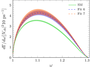
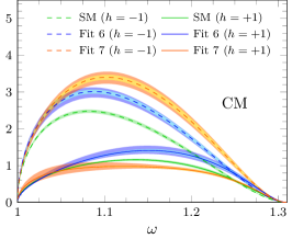
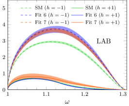
Figure 1: Left panel: $d\Gamma(\Lambda_{b}\to\Lambda_{c}\tau\bar{\nu}_{\tau})/d\omega$ differential decay width, as a function of $\omega$ and in units of $10|V_{cb}|^{2}{\rm ps}^{-1}$. We show SM predictions and full NP results obtained including all terms in Eq. (1) and using the Wilson coefficients from Fits 6 and 7 of Ref. Murgui et al. (2019). In the middle and right panels, we show the contributions to the $d\Gamma/d\omega$ corresponding to $\tau$ leptons with well defined helicities ($h=\pm 1)$ in the $W^{-}$CM and LAB reference systems, respectively. Uncertainty bands are obtained as detailed in the main text. For the NP results in the CM distributions, we also show the error bands corresponding to the form-factors uncertainties, which can be seen in lighter colors within the total error bands. In the case of the LAB frame, SM and Fit 6 positive-helicity distributions are practically indistinguishable.

	SM	Fit 6 Murgui et al. (2019)	Fit 7 Murgui et al. (2019)
$\Gamma(\Lambda_{b}\to\Lambda_{c}e(\mu)\bar{\nu}_{e(\mu)})/\left(10\times|V_{cb}|^{2}{\rm ps}^{-1}\right)$	$2.15\pm 0.08$	$-$	$-$
$\Gamma(\Lambda_{b}\to\Lambda_{c}\tau\bar{\nu}_{\tau})/\left(10\times|V_{cb}|^{2}{\rm ps}^{-1}\right)$	$0.715^{+0.014}_{-0.016}$	$0.872\pm 0.047$	$0.892\pm 0.051$
${\cal R}_{\Lambda_{c}}$	$0.332\pm 0.007$	$0.404\pm 0.022$	$0.414\pm 0.024$

Table 1: Total widths and ${\cal R}_{\Lambda_{c}}$ values associated to the distributions shown in the left panel of Fig. 1.

We start by showing in Fig. 1 results for the $d\Gamma(\Lambda_{b}\to\Lambda_{c}\tau\bar{\nu}_{\tau})/d\omega$ differential decay width. As we see in the left panel, Fits 6 and 7 give very similar results for $d\Gamma/d\omega$ and they become indistinguishable once the full uncertainty band is taken into account. Thus, by looking at the $d\Gamma/d\omega$ differential decay width (or the integrated decay width for that matter, as can be seen in Table 1) one could not decide which fit, and thus what NP terms, would be preferable to explain the data. As compared to our partial results of Ref. Penalva et al. (2019), we find a quite significant reduction of the error bands of the NP distributions thanks to having considered here the statistical correlations between the Wilson coefficients.

In Fig. 1, we also show the separate contributions to $d\Gamma/d\omega$ corresponding to $\tau$ leptons with well defined helicity ($h=\pm 1$) measured either in the CM (middle panel) or the LAB (right panel) reference systems. In the latter case there is no clear distinction (once the full error band is taken into account) between the predictions corresponding to Fits 6 and 7. The situation clearly improves for the case of well defined helicities in the CM system where the predictions from the two fits can be told apart in most of the $\omega$ range. However, polarized distributions are very challenging measurements because of the presence of undetected neutrinos, so next we examine other possibilities.

Fortunately, things improve considerably when one looks at the observables related to the CM $d^{2}\Gamma/(d\omega d\cos\theta_{\ell})$ and LAB unpolarized $d^{2}\Gamma/(d\omega dE_{\ell})$ double differential distributions. In Figs. 2 and 3 we show, respectively, the results for the $a_{i=0,1,2}$ and $c_{i=0,1,2}$ dimensionless coefficients that determine those distributions (Eqs. (18) and (21)). With the exception of $a_{0}$, the rest of these functions allow a clear distinction between NP Fits 6 and 7 that otherwise predict the same $d\Gamma/d\omega$ differential and total decay widths. We also display predictions, in the bottom panel of Fig. 2, for the commonly used forward-backward asymmetry ${\cal A}_{FB}$, which features and $\omega-$behaviour are strongly determined by $a_{1}$. If LFUV were experimentally established for the $\Lambda_{b}\to\Lambda_{c}$ semileptonic decays, the analysis of these observables would clearly help in establishing what kind of NP was needed to reproduce experimental data.

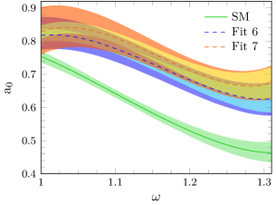
Figure 2: Top: CM angular expansion coefficients $a_{0},a_{1}$ and $a_{2}$ for the unpolarized $d^{2}\Gamma[\Lambda_{b}\to\Lambda_{c}\tau\bar{\nu}_{\tau}]/(d\omega d\cos\theta_{\ell})$ differential decay width (Eqs. (17) and (18)), as a function of $\omega$. Bottom: forward-backward asymmetry, ${\cal A}_{FB}=a_{1}/(2a_{0}+2a_{2}/3)$. We show SM and full results, the latter evaluated including all NP terms in Eq. (1) and using the Wilson coefficients from Fits 6 and 7 of Ref. Murgui et al. (2019). Uncertainty bands are obtained as explained in the main text. For NP results we also show the error bands corresponding to the form-factors uncertainties, which can be seen in lighter colors within the total error bands.

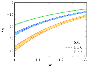
Figure 3: LAB charged lepton energy expansion coefficients $c_{0},c_{1}$ and $c_{2}$ (Eq. (21)) for the unpolarized $d^{2}\Gamma[\Lambda_{b}\to\Lambda_{c}\tau\bar{\nu}_{\tau}]/(d\omega dE_{\ell})$ differential decay width. Details as in Fig. 2.

Another way of presenting the results in Figs. 2 and 3 is by showing the ratios of the quantities obtained including NP over their SM values. This is done for $a_{1}$ and $c_{2}$ in Fig. 4. We observe that the $(c_{2})_{\rm NP}/(c_{2})_{\rm SM}$ ratio, depicted in the left-top panel of Fig. 4, is almost constant having a very mild $\omega$ dependence. However, it clearly distinguishes NP Fit 6 from Fit 7 and the two of them from the SM value of 1. We reached the same conclusions in our previous analysis of Ref. Penalva et al. (2019), but as it was the case with $d\Gamma/d\omega$, the proper consideration of the Wilson’s coefficient statistical correlations drastically reduces the errors in the predictions for this ratio, which sharpens the NP discriminating power of this observable. Similar results would be obtained for other ratios with the one for $a_{1}$, seen in the right-top panel of Fig. 4, showing the stronger $\omega$ dependence. As seen in Figs. 2 and 3, $a_{1}(\omega)$ is the only function, of those shown in these two figures, that presents a change of sign for the SM and the two NP scenarios analyzed in this work. This behaviour of $a_{1}$ explains the singularities in the NP ratios since, for each model, the zeros of $a_{1}$ occur at different positions within the physical interval $[1,\omega_{\rm max}]$. This strong $\omega-$dependence of the $(a_{1})_{\rm NP}/(a_{1})_{\rm SM}$ ratio provides an additional NP-testing tool, which could be used when future accurate measurements are available.

An alternative to this latter ratio that can be obtained just from pure experimental data is the following. Assuming that NP affects only the third generation of leptons, $a_{1}$ for $\ell=e,\mu$ (that can be considered as massless to a high degree of approximation) is a pure SM result, and the ratio $(a_{1})_{\tau}^{\rm NP}/(a_{1})_{\ell=e,\mu}^{\rm SM}$ can be measured from the asymmetry between the number of events observed for $\theta_{\ell}\in[0,\pi/2]$ and for $\theta_{\ell}\in[\pi/2,\pi]$,

$$\frac{(a_{1})_{\tau}^{\rm NP}(\omega)\rule{0.0pt}{12.48604pt}}{\rule{0.0pt}{12.48604pt}(a_{1})_{\ell=e,\mu}^{\rm SM}(\omega)}=\left(1-\frac{m_{\tau}^{2}}{q^{2}}\right)^{-2}\ \frac{\bigintss_{0}^{1}d\cos\theta_{\ell}\left[\frac{d^{2}\Gamma[\Lambda_{b}\to\Lambda_{c}\tau\bar{\nu}_{\tau}]}{d\omega d\cos\theta_{\ell}}(\omega,\theta_{\ell})\right]-\bigintss_{-1}^{0}d\cos\theta_{\ell}\left[\frac{d^{2}\Gamma[\Lambda_{b}\to\Lambda_{c}\tau\bar{\nu}_{\tau}]}{d\omega d\cos\theta_{\ell}}(\omega,\theta_{\ell})\right]\rule{0.0pt}{12.48604pt}}{\rule{0.0pt}{12.48604pt}\bigintss_{0}^{1}d\cos\theta_{\ell}\left[\frac{d^{2}\Gamma[\Lambda_{b}\to\Lambda_{c}e(\mu)\bar{\nu}_{e(\mu)}]}{d\omega d\cos\theta_{\ell}}(\omega,\theta_{\ell})\right]-\bigintss_{-1}^{0}d\cos\theta_{\ell}\left[\frac{d^{2}\Gamma[\Lambda_{b}\to\Lambda_{c}e(\mu)\bar{\nu}_{e(\mu)}]}{d\omega d\cos\theta_{\ell}}(\omega,\theta_{\ell})\right]}$$ (32)

This ratio is shown in the left-bottom panel of Fig. 4. Since $(a_{1})_{\ell=e,\mu}^{\rm SM}(\omega)$ does not vanish for $\omega>1$ (see Fig. 1 of Ref. Penalva et al. (2019)), no divergence appears in this case. In the insert to this latter panel we amplify the $\omega\in[1,1.2]$ region to better show the discriminating power of this observable close to zero recoil.

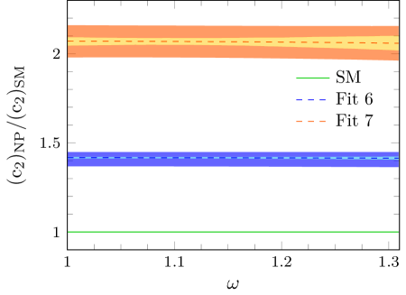
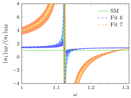
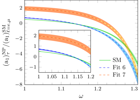
Figure 4: Top: $(c_{2})_{\rm NP}/(c_{2})_{\rm SM}$ (left) and $(a_{1})_{\rm NP}/(a_{1})_{\rm SM}$ (right) ratios for $\Lambda_{b}\to\Lambda_{c}\tau\bar{\nu}_{\tau}$, as a function of $\omega$. Bottom: ${(a_{1})_{\tau}^{\rm NP}(\omega)}/{(a_{1})_{\ell=e,\mu}^{\rm SM}(\omega)}$ and ${\cal R}({\cal A}_{FB})$ ratios defined in Eqs. (32) and (33), respectively. In the inserts to these latter plots, we amplify the $\omega$ region close to zero recoil. In all cases, we show results for the Fits 6 and 7 of Ref. Murgui et al. (2019), and details of the uncertainties are as in Fig. 2.

To minimize experimental and theoretical uncertainties, both the numerator and the denominator of the right hand side of Eq. (32) can be normalized by $d\Gamma/d\omega$ for each decay mode. In this way, the ratio ${\cal R}({\cal A_{FB}})$, defined as

$${\cal R}({\cal A}_{FB})=\frac{({\cal A}_{FB})_{\tau}^{\rm NP}}{({\cal A}_{FB})_{\ell=e,\mu}^{\rm SM}\rule{0.0pt}{12.48604pt}}=\frac{\Big{[}\frac{a_{1}\rule{0.0pt}{8.74023pt}}{2a_{0}+2a_{2}/3}\Big{]}_{\tau}^{\rm NP}\rule{0.0pt}{12.48604pt}}{\rule{0.0pt}{12.48604pt}\Big{[}\frac{a_{1}\rule{0.0pt}{8.74023pt}}{2a_{0}+2a_{2}/3}\Big{]}_{\ell=e,\mu}^{\rm SM}}$$ (33)

can be measured by subtracting the number of events seen for $\theta_{\ell}\in[0,\pi/2]$ and for $\theta_{\ell}\in[\pi/2,\pi]$ and dividing by the total sum of observed events, in each of the $\Lambda_{b}\to\Lambda_{c}\tau\bar{\nu}_{\tau}$ and $\Lambda_{b}\to\Lambda_{c}e(\mu)\bar{\nu}_{e(\mu)}$ reactions. We expect this strategy should remove a good part of experimental normalization errors. We show the theoretical predictions for ${\cal R}({\cal A}_{FB})$ in the bottom-right panel of Fig. 4, where we see a significant reduction of uncertainties, and the potential of this ratio to establish the validity of the NP scenarios associated to Fit 7. To avoid confusion, we must warn the reader that ${\cal R}({\cal A_{FB}})$ introduced here is not related with a ratio of hadronic forward-backward asymmetries defined in Eq. (2.46) of Ref. Böer et al. (2019), and which is discussed in Fig.1 of that work. The angles used in Böer et al. (2019) are different to those employed in the present analysis.

To complete the analysis, we display in Figs. 5 and 6 additional predictions for the polarized CM $d^{2}\Gamma/(d\omega d\cos\theta_{\ell})$ and LAB $d^{2}\Gamma/(d\omega dE_{\ell})$ distributions. As in the previous figures, we separate in all the observables the errors produced by the uncertainties in the LQCD determination of the form factors, which for the NP results are not negligible at all, and become even dominant in certain cases. In Fig. 5, we show the CM angular coefficients for positive and negative helicities, $a_{i=0,1,2}(h=\pm 1)$, which explicit expressions in terms of the $\widetilde{W}$ SFs were compiled in Eq. (25). Even taking uncertainties into account, Fits 6 and 7 provide distinctive predictions that also differ from the SM results. We see that $(h=+1)$ and $(h=-1)$ coefficients are comparable in size, and we systematically find

$$\left|a_{0,1,2}^{\rm NP-Fit\ 7}(h=-1)\right|\geq\left|a_{0,1,2}^{\rm NP-Fit\ 6}(h=-1)\right|\geq\left|a_{0,1,2}^{\rm SM}(h=-1)\right|$$ (34)

except for $a_{0}(h=-1)$ in a narrow region, $\omega=1-1.03$, where the NP Fit 6 and 7 predictions agree within errors. In the case of $a_{0}(h=+1)$ and $a_{1}(h=+1)$, roughly, NP Fit 6 values are greater than the Fit 7 ones, with SM results in the middle. Note that the partial integrated rates, $d\Gamma/d\omega$ shown in Fig. 1, are not sensitive to the $a_{1}-$contributions, and therefore having access to the detailed angular dependence provides very valuable additional information. We also see large cancellations in $a_{2}=a_{2}(h=+1)+a_{2}(h=-1)$, which become total, both at zero recoil and at the end of the phase space, where the sum $a_{2}$ vanishes. Actually for $\omega=\omega_{\rm max}$, $|a_{2}(h=\pm 1)|$ are as big as $a_{0}(h=\pm 1)$.

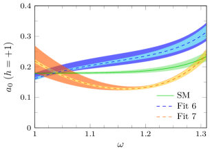
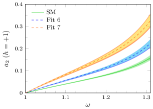
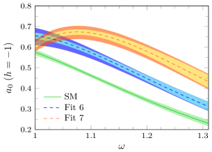
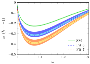
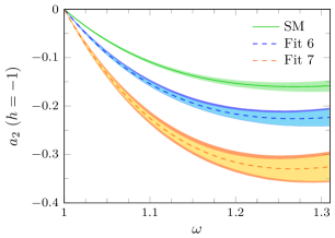
Figure 5: CM angular coefficients for positive and negative helicities $\left(a_{i=0,1,2}(h=\pm 1)\right)$ for the $\tau-$mode $\Lambda_{b}\to\Lambda_{c}$ semileptonic decay, as a function of $\omega$. Details as in Fig. 2.

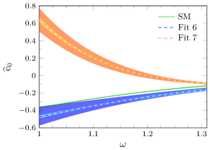
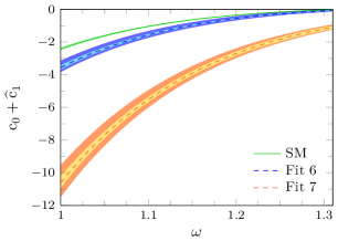
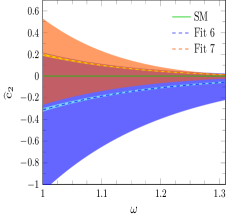
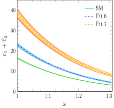
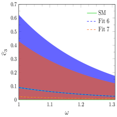
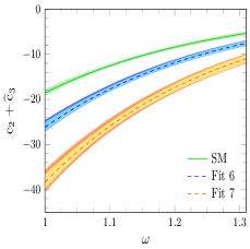
Figure 6: LAB charged lepton energy expansion coefficients $\widehat{c}_{i=0,1,2,3}$ (Eqs. (26) and (27)) for the polarized $d^{2}\Gamma[\Lambda_{b}\to\Lambda_{c}\tau\bar{\nu}_{\tau}]/(d\omega dE_{\ell})$ differential decay width. We also show the $(c_{0}+\widehat{c}_{1})$, $(c_{1}+\widehat{c}_{2})$ and $(c_{2}+\widehat{c}_{3})$ sums in the third top, second and fourth bottom panels, respectively. Details as in Fig. 2.

In Fig. 6 we show the $\widehat{c}_{i=0,1,2,3}$ coefficients, given in Eq. (27), that appear in the expression for the polarized LAB $d^{2}\Gamma/(d\omega dE_{\ell})$ double differential decay width. Taking into account the uncertainty bands, dominated by the errors of the Wilson coefficients, only $\widehat{c}_{0}$ and $\widehat{c}_{1}$ can be used to distinguish between NP Fits 6 and 7, while only Fit 7 predicts a result in clear disagreement with SM expectations. We see NP Fits 6 and 7 predictions for these two coefficients have even opposite signs, and the differences are enhanced in the sum $(c_{0}+\widehat{c}_{1})$, which is the coefficient of the linear $E_{\ell}$ term in Eq. (26).

The other two observables $\widehat{c}_{2}$ and $\widehat{c}_{3}$ are of little use for the current analysis, because the results of Fits 6 and 7 overlap and, furthermore, these coefficients are around two orders of magnitude lower than $c_{1}$ and $c_{2}$, respectively. One should note that $\widehat{c}_{2}$ and $\widehat{c}_{3}$ are proportional to the tensor-diagonal $\widetilde{W}^{T}_{2,4}$ and tensor-interference $\widetilde{W}_{I_{3},I_{5},I_{6}}$ SFs, and therefore both are zero in the SM. Moreover, for the NP scenarios associated to Fit 6 and 7 of Ref. Murgui et al. (2019), these two coefficients of the unpolarized distribution are negligible, since for both fits $|C_{T}|$ is already of the order of $10^{-2}$, and compatible with zero, $C_{T}=0.01^{+0.09}_{-0.07}$ and $-0.02^{+0.08}_{-0.07}$, respectively.

However, it is important to stress that $\widehat{c}_{2}$ and $\widehat{c}_{3}$ are optimal observables to restrict the validity of NP schemes with high tensor contributions. As a matter of example,

$$\frac{\widehat{c}_{3}(\omega)}{c_{2}(\omega)}=\frac{32\widetilde{W}_{2}^{T}}{\widetilde{W}_{2}-\rule{0.0pt}{12.48604pt}16\widetilde{W}_{2}^{T}}=\frac{32\widetilde{W}_{2}^{T}}{\rule{0.0pt}{12.48604pt}\widetilde{W}_{2}}+\cdots=-32x+{\cal O}(\Lambda_{QCD}/m_{b,c}),\quad x=\frac{2|C_{T}|^{2}}{|C_{V}|^{2}+|C_{A}|^{2}}$$ (35)

where we have made used that $\widetilde{W}_{2}^{T}/\widetilde{W}_{2}=-x+{\cal O}(\Lambda_{QCD}/m_{b,c})$, as deduced from Eq. (29).

On the other hand, the small NP tensor contribution for Fits 6 and 7, together with the heavy quark limit relations of Eq. (29), explains the flat $\omega-$behavior of the $(c_{2})_{NP}/(c_{2})_{SM}$ ratio seen in Fig. 4. If one neglects $\widetilde{W}^{T}_{2}$, the coefficient $c_{2}$ is proportional to $\widetilde{W}_{2}$. The linear $C_{V_{R}}$ terms, that could induce a non-zero $\omega$ dependence in $(\widetilde{W}_{2})_{NP}/(\widetilde{W}_{2})_{SM}$, cancel to order ${\cal O}(\Lambda_{\rm QCD}/m_{b,c})$.

Finally, in Fig. 7, we present ${\cal R}_{\Lambda_{c}}$ as a function of ${\cal R}_{D}$ obtained using NP Fit 6 (left) and 7 (middle) $\chi^{2}-$weighted samples of Wilson coefficients provided by the authors of Ref. Murgui et al. (2019). In Fig. 7, we include sets beyond the $1\sigma$ ones. For illustration purposes, we also show the results of Ref. Murgui et al. (2019) for the ratio ${\cal R}_{D^{*}}$, which allows us to highlight the clear correlation between these three LFUV observables. Note that SM predictions for the ${\cal R}_{D}^{\rm SM}=0.300\pm 0.05$ and ${\cal R}_{D^{*}}^{\rm SM}=0.251\pm 0.004$ ratios are below the ranges considered, while ${\cal R}^{\rm SM}_{\Lambda_{c}}=0.332\pm 0.008$. In the right panel of Fig. 7, we show, for each of the Wilson coefficient sets used in the left and middle panels, the $\chi^{2}-$variations against the corresponding changes induced in the ${\cal R}_{\Lambda_{c}}$ ratio. Both, Fit 6 and Fit 7 $\chi^{2}$ functions grow from their minimum values, and the $\Delta\chi^{2}=1$, $\Delta\chi^{2}=2.71$, $\Delta\chi^{2}=6.63,\cdots$ increments can be used to determine the 68% ($1\sigma$), 90% ($2\sigma$), 99%($3\sigma$), $\cdots$ CL intervals of the NP predictions for ${\cal R}_{D}$, ${\cal R}_{D^{*}}$ and ${\cal R}_{\Lambda_{c}}$.

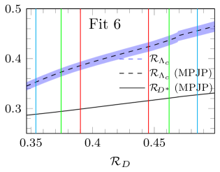
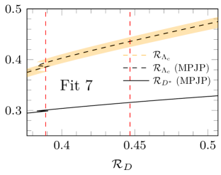
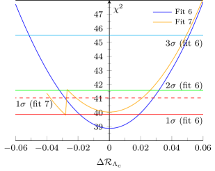
Figure 7: Left/middle panel: NP Fits 6 and 7 results for ${\cal R}_{\Lambda_{c}}$ and ${\cal R}_{D^{*}}$ as a function of ${\cal R}_{D}$ for different $\chi^{2}-$weighted samples of Wilson coefficients. Black solid and dashed curves, labeled as MPJP, stand for the results of Ref. Murgui et al. (2019) provided by the authors of that work Peñuelas and Murgui . The blue and orange dashed lines (indistinguishable from the MPJP predictions) correspond to the current numerical evaluation of ${\cal R}_{\Lambda_{c}}$ for Fits 6 and 7, respectively, with the shaded bands showing the 68% CL uncertainties inherited from the LQCD determination of the form-factors Detmold et al. (2015); Datta et al. (2017). Right panel: Chi-square values Murgui et al. (2019); Peñuelas and Murgui for each set of Wilson coefficients (sWC) used in the left and middle panels, and represented in this plot by $\Delta{\cal R}_{\Lambda_{c}}={\cal R}_{\Lambda_{c}}^{\rm sWC}-{\cal R}_{\Lambda_{c}}^{\min}$, with ${\cal R}_{\Lambda_{c}}^{\min}=0.405$ and 0.415 for Fits 6 and 7, respectively.

IV Conclusions

We have included the NP tensor term, and all the interference contributions associated with it, in our general formalism for semileptonic decays initially introduced in Ref. Penalva et al. (2019). In this way, all the NP effective Hamiltonians that are considered in LFUV studies with massless left-handed neutrinos have now been taken into account, including the possibility of violation of CP-symmetry due to the presence of complex Wilson coefficients. The scheme developed is totally general and it can be applied to any charged current semileptonic decay, involving any quark flavors or initial and final hadron states.

We have shown that a total of sixteen SFs ($\widetilde{W}$’s) are needed to fully describe the hadronic tensor. They are constructed out of the complex Wilson coefficients, that characterize the strength of the different NP terms, and the form factors needed to describe the genuine hadronic matrix elements. We have also derived general expressions for unpolarized and charged-lepton polarized CM $d^{2}\Gamma/(d\omega d\cos\theta_{\ell})$ and LAB $d^{2}\Gamma/(d\omega dE_{\ell})$ differential decay widths in terms of the $\widetilde{W}-$SFs. Unlike the unpolarized case, where all the accessible observables could be determined either from the CM or LAB distributions, we have pointed out that LAB and CM charged lepton helicity distributions should be used simultaneously, since in the polarized case, they provide complementary information. We have also shown that, even assuming that the NP terms affect only to the third lepton family, the strategy to obtain full polarized information for tau-mode decays from non-polarized $e/\mu$ and $\tau$ data is spoiled by the presence of NP tensor operators.

As a result of this general discussion, we have concluded that determining all NP parameters, with their complex phases, from a single type of decay is tough, even assuming that the hadronic form factors are known. This is because the experimental measurements of the required polarized decays are very challenging due to the presence of undetected neutrinos. We have argued it is therefore essential to simultaneously analyze data from various types of semileptonic decays (f.e. $\bar{B}\to D,\bar{B}\to D^{*}$, $\Lambda_{b}\to\Lambda_{c},\bar{B}_{c}\to\eta_{c},\bar{B}_{c}\to J/\Psi$…), considering both the $e/\mu$ and $\tau$ modes, and that the scheme presented in this work is a powerful tool to achieve this goal.

The general formalism developed has then been applied to update the analysis of the $\Lambda_{b}\to\Lambda_{c}\tau\bar{\nu}_{\tau}$ decay carried out in Ref. Penalva et al. (2019). We have found small numerical differences for central results, because of the little strength of the tensor terms in the NP scenarios originally considered in our previous work. However, the proper consideration of the Wilson’s coefficient statistical correlations has drastically reduced the errors in the new predictions, which have significantly improved the NP discriminating power of the present study. In addition, we have obtained full results for both CM and LAB charged lepton polarized distributions.

As in Ref. Penalva et al. (2019), we have shown the potential of the CM $d^{2}\Gamma/(d\omega d\cos\theta_{\ell})$ and LAB $d^{2}\Gamma/(d\omega dE_{\ell})$ distributions to distinguish between models, fitted to $b\to c\tau\bar{\nu}_{\tau}$ anomalies in the meson sector, that differ in the strengths of the NP terms but that otherwise give the same differential $d\Gamma/d\omega$ and integrated decay widths. In particular, the $a_{1}$ and $a_{2}$, and all three $c_{0},\,c_{1}$ and $c_{2}$ functions, associated with the non-polarized CM $d^{2}\Gamma/(d\omega d\cos\theta_{\ell})$ and LAB $d^{2}\Gamma/(d\omega dE_{\ell})$ distributions, respectively, are very well suited for that purpose, at least for the $\Lambda_{b}\to\Lambda_{c}$ semileptonic decay specifically studied in this work. For this baryon transition, we have also shown the great interest of the ratios $(a_{1})_{\tau}^{\rm NP}/(a_{1})_{\ell=e,\mu}^{\rm SM}$ and ${\cal R}({\cal A}_{FB})$ (Eqs. (32) and (33), respectively) which can be directly measured from the $(\theta_{\ell},\pi-\theta_{\ell})$ asymmetry of the experimental distributions. If LFUV is experimentally established for this decay, the analysis of all these observables can help in understanding what kind of NP is needed to explain the data. Finally, we have identified two coefficient functions, in the LAB polarized distribution, which theoretically should be very efficient in restricting the validity of NP schemes with a sizable tensor contribution, although we are aware of the difficulty of their measurement at present and in the near future.

Appendix A Lepton tensors

From Eq. (5), in the limit of massless neutrinos, we obtain

$$J^{L}_{(\alpha\beta)}(k,k^{\prime};h)[J^{L}_{(\rho\lambda)}(k,k^{\prime};h)]^{*}=\frac{1}{4}{\rm Tr}\Big{[}(\not{k}^{\prime}+m_{\ell})\Gamma_{(\alpha\beta)}(1-\gamma_{5})\not{k}\,\widetilde{\Gamma}_{(\rho\lambda)}P_{h}\Big{]},\qquad\widetilde{\Gamma}_{(\rho\lambda)}=\gamma^{0}\Gamma_{(\rho\lambda)}^{\dagger}\gamma^{0}.$$ (36)

The different $\Gamma_{(\alpha\beta)}$ and $\Gamma_{(\rho\lambda)}$ operators give rise to the following lepton tensors (we use the convention $\epsilon_{0123}=+1$ and $g_{\mu\nu}=(+,-,-,-)$)

$$L(k,k^{\prime};h) = \left(k\cdot k^{\prime}+h\,\,k\cdot s\right)/2,$$ (37)

$$L_{\alpha}(k,k^{\prime};h) = \frac{m_{\ell}}{2}k_{\alpha}+\frac{h}{2m_{\ell}}\left(k^{\prime}_{\alpha}\,k\cdot s-s_{\alpha}\,k\cdot k^{\prime}+i\epsilon_{\alpha\delta\eta\sigma}k^{\prime\delta}k^{\eta}s^{\sigma}\right),$$ (38)

$$L^{\prime}_{\rho\lambda}(k,k^{\prime};h) = \frac{i}{2}\left(k_{\rho}k^{\prime}_{\lambda}-k_{\lambda}k^{\prime}_{\rho}+i\epsilon_{\rho\lambda\delta\eta}k^{\prime\delta}k^{\eta}\right)+i\frac{h}{2}\left(k_{\rho}s_{\lambda}-k_{\lambda}s_{\rho}+i\epsilon_{\rho\lambda\delta\eta}s^{\delta}k^{\eta}\right),$$ (39)

$$L_{\alpha\rho}(k,k^{\prime};h) = \frac{1}{2}\left(k^{\prime}_{\alpha}k_{\rho}+k_{\alpha}k^{\prime}_{\rho}-g_{\alpha\rho}k\cdot k^{\prime}+i\epsilon_{\alpha\rho\delta\eta}k^{\prime\delta}k^{\eta}\right)-\frac{h}{2}\left(s_{\alpha}k_{\rho}+k_{\alpha}s_{\rho}-g_{\alpha\rho}k\cdot s+i\epsilon_{\alpha\rho\delta\eta}s^{\delta}k^{\eta}\right),$$ (40)

$$L_{\alpha\rho\lambda}(k,k^{\prime};h) = \frac{im_{\ell}}{2}\left(g_{\alpha\lambda}k_{\rho}-g_{\alpha\rho}k_{\lambda}+i\epsilon_{\alpha\rho\lambda\delta}k^{\delta}\right)$$ (41)

$$-\frac{ih}{2m_{\ell}}\Big{[}k^{\prime}_{\alpha}(s_{\rho}k_{\lambda}-s_{\lambda}k_{\rho})+k_{\alpha}(s_{\rho}k^{\prime}_{\lambda}-s_{\lambda}k^{\prime}_{\rho})+s_{\alpha}(k_{\rho}k^{\prime}_{\lambda}-k_{\lambda}k^{\prime}_{\rho})$$

$$\hskip 42.67912pt+(k\cdot k^{\prime})(g_{\alpha\rho}s_{\lambda}-g_{\alpha\lambda}s_{\rho})+(s\cdot k)(g_{\alpha\lambda}k^{\prime}_{\rho}-g_{\alpha\rho}k^{\prime}_{\lambda})\Big{]}$$

$$-\frac{h}{2m_{\ell}}\Big{[}(k\cdot k^{\prime})\epsilon_{\alpha\rho\lambda\delta}s^{\delta}+s_{\lambda}\epsilon_{\alpha\rho\delta\eta}k^{\prime\delta}k^{\eta}-s_{\rho}\epsilon_{\alpha\lambda\delta\eta}k^{\prime\delta}k^{\eta}+k_{\alpha}\epsilon_{\rho\lambda\delta\eta}s^{\delta}k^{\prime\eta}+k^{\prime}_{\alpha}\epsilon_{\rho\lambda\delta\eta}s^{\delta}k^{\eta}\Big{]},$$

$$L_{\alpha\beta\rho\lambda}(k,k^{\prime};h) = \frac{1}{2}L_{\alpha\beta\rho\lambda}(k,k^{\prime})+\frac{h}{2}L_{\alpha\beta\rho\lambda}(k,s),$$ (42)

which correspond to the $(\Gamma_{(\alpha\beta)},\Gamma_{(\rho\lambda)})=(1,1),(\gamma_{\alpha},1),(1,\sigma_{\rho\lambda}),(\gamma_{\alpha},\gamma_{\rho})$, $(\gamma_{\alpha},\sigma_{\rho\lambda})$, and $(\sigma_{\alpha\beta},\sigma_{\rho\lambda})$ combinations, respectively, and in Eq. (42)

$$L_{\alpha\beta\rho\lambda}(k,k^{\prime}) = g_{\beta\rho}(k_{\alpha}k^{\prime}_{\lambda}+k_{\lambda}k^{\prime}_{\alpha})-g_{\beta\lambda}(k_{\alpha}k^{\prime}_{\rho}+k_{\rho}k^{\prime}_{\alpha})-g_{\alpha\rho}(k_{\beta}k^{\prime}_{\lambda}+k_{\lambda}k^{\prime}_{\beta})+g_{\alpha\lambda}(k_{\beta}k^{\prime}_{\rho}+k_{\rho}k^{\prime}_{\beta})$$ (43)

$$+(k\cdot k^{\prime})(g_{\alpha\rho}g_{\beta\lambda}-g_{\alpha\lambda}g_{\beta\rho})+i\Big{(}k^{\prime}_{\alpha}\epsilon_{\beta\lambda\rho\delta}k^{\delta}-k^{\prime}_{\beta}\epsilon_{\alpha\lambda\rho\delta}k^{\delta}+k_{\rho}\epsilon_{\alpha\beta\lambda\delta}k^{\prime\delta}-k_{\lambda}\epsilon_{\alpha\beta\rho\delta}k^{\prime\delta}\Big{)}.$$

Appendix B Hadron tensors

We collect here the hadron tensors that should be contracted with the corresponding lepton ones, compiled in the previous appendix, to obtain $\overline{\sum}|{\cal M}|^{2}$. In Sec. II.2.1, we have addressed the diagonal $J_{H}^{\alpha}[J_{H}^{\rho}]^{*}$ case. In this appendix, we begin with the diagonal $J_{H}^{\alpha\beta}[J_{H}^{\rho\lambda}]^{*}$ tensor term, which it is also discussed in detail. The decomposition of the rest of the hadron tensors as linear combination of independent Lorentz (pseudo-)tensor structures is listed after, and it is obtained similarly to those in the two previous examples. The coefficients multiplying the (pseudo-)tensors are the $\widetilde{W}^{\prime}s$ SFs, which depend on $q^{2}$ and the hadron masses. As mentioned in the Introduction, there appear 16 $\widetilde{W}^{\prime}s$ SFs, which are constructed out of NP complex Wilson coefficients and the genuine hadronic responses ($W^{\prime}s$). The latter ones are determined by the matrix elements of the involved hadron operators, which for each particular decay are parametrized in terms of form-factors.

• The diagonal contribution of the tensor operator $O_{H}^{\alpha\beta}$ gives rise to a (pseudo-)tensor of four indices

  $$W^{\alpha\beta\rho\lambda}(p,q,C_{T})=|C_{T}|^{2}\overline{\sum_{r,r^{\prime}}}\langle H_{c};p^{\prime},r^{\prime}|\bar{c}(0)\sigma^{\alpha\beta}(1-\gamma_{5})b(0)|H_{b};p,r\rangle\langle H_{c};p^{\prime},r^{\prime}|\bar{c}(0)\sigma^{\rho\lambda}(1-\gamma_{5})b(0)|H_{b};p,r\rangle^{*},$$ (44)

  which contracted with the lepton tensor $L_{\alpha\beta\rho\lambda}(k,k^{\prime};h)$ in Eq. (42) provides the contribution to the differential decay rate. Note that by construction $W^{\alpha\beta\rho\lambda}(p,q,C_{T})=W^{\rho\lambda\alpha\beta*}(p,q,C_{T})$, and hence, if

  $$W^{\alpha\beta\rho\lambda} = \frac{1}{2}[W^{\alpha\beta\rho\lambda}+W^{\rho\lambda\alpha\beta}]+\frac{1}{2}[W^{\alpha\beta\rho\lambda}-W^{\rho\lambda\alpha\beta}]$$ (45)

  $$= \frac{1}{2}[W^{\alpha\beta\rho\lambda}+W^{\alpha\beta\rho\lambda*}]+\frac{1}{2}[W^{\alpha\beta\rho\lambda}-W^{\alpha\beta\rho\lambda*}]\equiv W^{\alpha\beta\rho\lambda}_{(s)}+W^{\alpha\beta\rho\lambda}_{(a)},$$

  the symmetric and antisymmetric, under the $(\alpha\beta)\leftrightarrow(\rho\lambda)$ exchange, parts become real and purely imaginary, respectively. Now introducing the decomposition ($T=\sigma$, $pT=\sigma\gamma_{5}$)

  $$W^{\alpha\beta\rho\lambda}(p,q,C_{T})=|C_{T}|^{2}\left[W^{\alpha\beta\rho\lambda}_{TT}(p,q)+W^{\alpha\beta\rho\lambda}_{pTpT}(p,q)-W^{\alpha\beta\rho\lambda}_{TpT}(p,q)-W^{\alpha\beta\rho\lambda}_{pTT}(p,q)\right],$$ (46)

  and using parity and time-reversal, as in Eqs. (11) and (12), we conclude that $W_{TT}^{\alpha\beta\rho\lambda}$ and $W_{pTpT}^{\alpha\beta\rho\lambda}$ ($W_{TpT}^{\alpha\beta\rho\lambda}$ and $W_{pTT}^{\alpha\beta\rho\lambda}$) are real tensors (imaginary pseudotensors). Indeed, we can identify

  $$W^{\alpha\beta\rho\lambda}_{(s)} = |C_{T}|^{2}\left[W^{\alpha\beta\rho\lambda}_{TT}(p,q)+W^{\alpha\beta\rho\lambda}_{pTpT}(p,q)\right],$$ (47)

  $$W^{\alpha\beta\rho\lambda}_{(a)} = -|C_{T}|^{2}\left[W^{\alpha\beta\rho\lambda}_{TpT}(p,q)+W^{\alpha\beta\rho\lambda}_{pTT}(p,q)\right],$$ (48)

  and conclude that the tensors/pseudotensors should be $(\alpha\beta)\leftrightarrow(\rho\lambda)$ symmetric/antisymmetric. In addition, both of them should be obviously antisymmetric under $\alpha\leftrightarrow\beta$ and $\rho\leftrightarrow\lambda$ exchanges. There is still a large freedom, and a priori 5 (8) different four-index tensor (pseudotensor) structures, meeting all the above requirements, can be used to construct $W^{\alpha\beta\rho\lambda}_{(s)}$ ($W^{\alpha\beta\rho\lambda}_{(a)}$). An important simplification is found recalling that

  $$\gamma_{5}\sigma^{\alpha\beta}=-\frac{i}{2}\epsilon^{\alpha\beta\delta\eta}\sigma_{\delta\eta},\,$$ (49)

  which can be used to relate $W^{\alpha\beta\rho\lambda}_{(s)}$ and $W^{\alpha\beta\rho\lambda}_{(a)}$. We find

  $$W^{\alpha\beta\rho\lambda}=W^{\alpha\beta\rho\lambda}_{(s)}-\frac{i}{2}\epsilon^{\rho\lambda}_{\ \ \delta\eta}W^{\alpha\beta\delta\eta}_{(s)},$$ (50)

  which implies that the total tensor can be expressed using only the five real SFs that appear in the Lorentz decomposition of $W^{\alpha\beta\rho\lambda}_{(s)}$.

  $$W^{\alpha\beta\rho\lambda} = |C_{T}|^{2}\Bigg{\{}W_{1}^{T}\Big{[}(g^{\alpha\rho}g^{\beta\lambda}-g^{\alpha\lambda}g^{\beta\rho})-i\epsilon^{\rho\lambda\alpha\beta}\Big{]}+\frac{W_{2}^{T}}{M^{2}}\Big{[}(g^{\alpha\rho}p^{\beta}p^{\lambda}-g^{\alpha\lambda}p^{\beta}p^{\rho}-g^{\beta\rho}p^{\alpha}p^{\lambda}+g^{\beta\lambda}p^{\alpha}p^{\rho})$$ (52)

  $$-i\Big{(}\epsilon^{\rho\lambda\alpha\delta}p^{\beta}p_{\delta}-\epsilon^{\rho\lambda\beta\delta}p^{\alpha}p_{\delta}\Big{)}\Big{]}+\frac{W_{3}^{T}}{M^{2}}\Big{[}(g^{\alpha\rho}q^{\beta}q^{\lambda}-g^{\alpha\lambda}q^{\beta}q^{\rho}-g^{\beta\rho}q^{\alpha}q^{\lambda}+g^{\beta\lambda}q^{\alpha}q^{\rho})$$

  $$-i\Big{(}\epsilon^{\rho\lambda\alpha\delta}q^{\beta}q_{\delta}-\epsilon^{\rho\lambda\beta\delta}q^{\alpha}q_{\delta}\Big{)}\Big{]}+\frac{W_{4}^{T}}{M^{2}}\Big{[}\Big{[}g^{\alpha\rho}(p^{\beta}q^{\lambda}+p^{\lambda}q^{\beta})-g^{\alpha\lambda}(p^{\beta}q^{\rho}+p^{\rho}q^{\beta})-g^{\beta\rho}(p^{\alpha}q^{\lambda}+p^{\lambda}q^{\alpha})$$

  $$+g^{\beta\lambda}(p^{\alpha}q^{\rho}+p^{\rho}q^{\alpha})\Big{]}-i\Big{(}\epsilon^{\rho\lambda\alpha\delta}(p^{\beta}q_{\delta}+q^{\beta}p_{\delta})-\epsilon^{\rho\lambda\beta\delta}(p^{\alpha}q_{\delta}+q^{\alpha}p_{\delta})\Big{)}\Big{]}$$

  $$+\frac{W_{5}^{T}}{M^{4}}\Big{[}(p^{\alpha}q^{\beta}-p^{\beta}q^{\alpha})(p^{\rho}q^{\lambda}-p^{\lambda}q^{\rho})-i(p^{\alpha}q^{\beta}-p^{\beta}q^{\alpha})\epsilon^{\rho\lambda\delta\eta}p_{\delta}q_{\eta}\Big{]}\Bigg{\}}.$$

  Requiring now that the pseudotensor part of $W^{\alpha\beta\rho\lambda}$ should be $(\alpha\beta)\leftrightarrow(\rho\lambda)$ antisymmetric, we find further constrains for the $W_{1,2,3,4,5}^{T}$ since they should satisfy

  $$M^{2}W_{1}^{T}\Big{[}\epsilon^{\rho\lambda\alpha\beta}+\epsilon^{\alpha\beta\rho\lambda}\Big{]}+W_{2}^{T}\Big{[}\Big{(}\epsilon^{\rho\lambda\alpha\delta}p^{\beta}p_{\delta}-\epsilon^{\rho\lambda\beta\delta}p^{\alpha}p_{\delta}\Big{)}+\Big{(}\epsilon^{\alpha\beta\rho\delta}p^{\lambda}p_{\delta}-\epsilon^{\alpha\beta\lambda\delta}p^{\rho}p_{\delta}\Big{)}\Big{]}$$

  $$+W_{3}^{T}\Big{[}\Big{(}\epsilon^{\rho\lambda\alpha\delta}q^{\beta}q_{\delta}-\epsilon^{\rho\lambda\beta\delta}q^{\alpha}q_{\delta}\Big{)}+\Big{(}\epsilon^{\alpha\beta\rho\delta}q^{\lambda}q_{\delta}-\epsilon^{\alpha\beta\lambda\delta}q^{\rho}q_{\delta}\Big{)}\Big{]}$$

  $$+W_{4}^{T}\Big{[}\Big{(}\epsilon^{\rho\lambda\alpha\delta}(p^{\beta}q_{\delta}+q^{\beta}p_{\delta})-\epsilon^{\rho\lambda\beta\delta}(p^{\alpha}q_{\delta}+q^{\alpha}p_{\delta})\Big{)}+\Big{(}\epsilon^{\alpha\beta\rho\delta}(p^{\lambda}q_{\delta}+q^{\lambda}p_{\delta})-\epsilon^{\alpha\beta\lambda\delta}(p^{\rho}q_{\delta}+q^{\rho}p_{\delta})\Big{)}\Big{]}$$

  $$+W_{5}^{T}\Big{[}(p^{\alpha}q^{\beta}-p^{\beta}q^{\alpha})\epsilon^{\rho\lambda\delta\eta}p_{\delta}q_{\eta}+(p^{\rho}q^{\lambda}-p^{\lambda}q^{\rho})\epsilon^{\alpha\beta\delta\eta}p_{\delta}q_{\eta}\Big{]}=0.$$ (53)

  The above equation can be rewritten as

  $$\epsilon^{\alpha\beta\rho\lambda}\Big{[}2M^{2}W_{1}^{T}+p^{2}W_{2}^{T}+q^{2}W_{3}^{T}+2(p\cdot q)W_{4}^{T}\Big{]}+q^{2}p^{\rho}\epsilon^{\alpha\beta\delta\lambda}p_{\delta}\,W_{5}^{T}=0,$$ (54)

  where we have used that

  $$\epsilon^{\alpha\beta\rho\delta}a_{\delta}b^{\lambda}-\epsilon^{\alpha\beta\lambda\delta}a_{\delta}b^{\rho}+\epsilon^{\rho\lambda\alpha\delta}a_{\delta}b^{\beta}-\epsilon^{\rho\lambda\beta\delta}a_{\delta}b^{\alpha}=(a\cdot b)\epsilon^{\alpha\beta\rho\lambda}.$$ (55)

  Taking into account that the two tensors that appear in Eq. (54) are independent, we deduce

  $$2M^{2}W_{1}^{T}+p^{2}W_{2}^{T}+q^{2}W_{3}^{T}+2(p\cdot q)W_{4}^{T}=0,\qquad W_{5}^{T}=0.$$ (56)

  The first of the above equations can be used to re-write $W_{1}^{T}$ in terms of $W^{T}_{2,3,4}$. Nevertheless, the contraction of the tensor that multiplies $W_{1}^{T}$ in the decomposition of Eq. (52) with the lepton tensor $L_{\alpha\beta\rho\lambda}(k,k^{\prime};h)$ defined in Eq. (42) vanishes identically. Hence, the contribution of $W^{\alpha\beta\rho\lambda}$ to $\overline{\sum}|{\cal M}|^{2}$ is given just in terms of three ($W_{2}^{T}$, $W_{3}^{T}$, $W_{4}^{T}$) real SFs.

  Finally, we absorb the common factor $|C_{T}|^{2}$, by redefining $\widetilde{W}^{T}_{1,2,3,4}=|C_{T}|^{2}W^{T}_{1,2,3,4}$.

• The diagonal contribution of the operator $O_{H}$ gives rise to the scalar

  $$W(p,q)=\widetilde{W}_{SP}(q^{2})=|C_{S}|^{2}\overline{\sum_{r,r^{\prime}}}|\langle H_{c};p^{\prime},r^{\prime}|\bar{c}(0)b(0)|H_{b};p,r\rangle|^{2}+|C_{P}|^{2}\overline{\sum_{r,r^{\prime}}}|\langle H_{c};p^{\prime},r^{\prime}|\bar{c}(0)\gamma_{5}b(0)|H_{b};p,r\rangle|^{2},$$ (57)

  which should be multiplied by the scalar lepton term of Eq. (37). Note that the $C_{S}C_{P}^{*}$ and $C_{P}C_{S}^{*}$ interference terms would give rise to purely imaginary pseudoscalars, which necessarily vanish because they cannot be constructed out of the $p$ and $q$ four-vectors alone.

• The $O_{H}^{\alpha}$ and $O_{H}$ interference contribute to the decay width as $2{\rm Re}\left[W^{\alpha}(p,q,C_{V,A,S,P})L_{\alpha}(k,k^{\prime};h)\right]$, with the $L_{\alpha}(k,k^{\prime};h)$ lepton tensor defined in Eq. (38) and

  $$W^{\alpha}(p,q,C_{V,A,S,P})=\overline{\sum_{r,r^{\prime}}}\langle H_{c};p^{\prime},r^{\prime}|(C_{V}V^{\alpha}-C_{A}A^{\alpha})|H_{b};p,r\rangle\langle H_{c};p^{\prime},r^{\prime}|\bar{c}(0)(C_{S}-C_{P}\gamma_{5})b(0)|H_{b};p,r\rangle^{*},$$ (58)

  and its treatment is similar to that discussed for $J_{H}^{\alpha}[J_{H}^{\rho}]^{*}$ in Sec. II.2.1, with the equivalence $(VV)\leftrightarrow(VS)$, $(AA)\leftrightarrow(AP)$, $(V\!A)\leftrightarrow(VP)$ and $(AV)\leftrightarrow(AS)$. Thus, we find

  $$W^{\alpha}(p,q,C_{V,A,S,P}) = \frac{1}{2M}\left(\widetilde{W}_{I1}p^{\alpha}+\widetilde{W}_{I2}q^{\alpha}\right),$$ (59)

  $$\widetilde{W}_{I1,I2}(q^{2},C_{V,A,S,P}) = C_{V}C^{*}_{S}W^{VS}_{I1,I2}(q^{2})+C_{A}C^{*}_{P}W^{AP}_{I1,I2}(q^{2}),$$ (60)

  with all four $W^{VS,AP}_{I1,I2}$ SFs being real, and where we have used an obvious notation in which $W_{I1,I2}^{VS}$, and $W_{I1,I2}^{AP}$ should be obtained from the $VS$ and $AP$ matrix elements. Note that the odd parity $VP$ and $AS$ terms would give rise to purely imaginary pseudo-vectors, which necessarily vanish because they cannot be constructed out of $p$ and $q$ alone. Thus, the total contribution to $\overline{\sum}|{\cal M}|^{2}$ of these pieces is given by

  $${\rm Re}\left[\left(\frac{\widetilde{W}_{I1}}{M}p^{\alpha}+\frac{\widetilde{W}_{I2}}{M}q^{\alpha}\right)L_{\alpha}(k,k^{\prime};h)\right].$$ (61)

  For real Wilson coefficients, the $\widetilde{W}_{I1,I2}$ SFs are real, and taking the real part in Eq. (61) amounts to remove the Levi-Civita term of $L_{\alpha}(k,k^{\prime};h)$, recovering in this way the result of Ref. Penalva et al. (2019) identifying $\widetilde{W}_{I1,I2}$ with $W_{I1,I2}$ introduced in the latter reference.

• The $O_{H}$ and $O_{H}^{\rho\lambda}$ interference contribute to the decay width as $2{\rm Re}\left[W^{\prime\rho\lambda}(p,q,C_{S,P,T})L^{\prime}_{\rho\lambda}(k,k^{\prime};h)\right]$, with the $L^{\prime}_{\rho\lambda}(k,k^{\prime};h)$ lepton tensor defined in Eq. (39) and

  $$W^{\prime\rho\lambda}(p,q,C_{S,P,T})=C_{T}^{*}\overline{\sum_{r,r^{\prime}}}\langle H_{c};p^{\prime},r^{\prime}|\bar{c}(0)(C_{S}-C_{P}\gamma_{5})b(0)|H_{b};p,r\rangle\langle H_{c};p^{\prime},r^{\prime}|\bar{c}(0)\sigma^{\rho\lambda}(1-\gamma_{5})b(0)|H_{b};p,r\rangle^{*}.$$ (62)

  We use Lorentz, parity and time-reversal transformations, as explained in Eqs. (11) and (12), to deduce that the $ST$ and $PpT$ ($SpT$ and $PT$) tensors are purely imaginary (real) antisymmetric tensors (pseudotensors). In addition, the $SpT$ and $PT$ pseudotensors can be related to the $ST$ and $PpT$ tensors thanks to Eq. (49). We finally find

  $$W^{\prime\rho\lambda}(p,q,C_{S,P,T}) = \frac{\widetilde{W}_{I3}}{2M^{2}}\left[\epsilon^{\rho\lambda\delta\eta}p_{\delta}q_{\eta}+i(p^{\rho}q^{\lambda}-p^{\lambda}q^{\rho})\right],$$

  $$\widetilde{W}_{I3}(q^{2},C_{S,P,T}) = C_{T}^{*}\left(C_{S}W_{I3}^{ST}(q^{2})+C_{P}W_{I3}^{PpT}(q^{2})\right),$$ (63)

  and the real $W_{I3}^{ST}$ and $W_{I3}^{PpT}$ SFs, obviously, deduced from the decompositions

  $$W^{\prime PpT}_{\rho\lambda}(p,q) = \overline{\sum_{r,r^{\prime}}}\langle H_{c};p^{\prime},r^{\prime}|\bar{c}(0)\gamma_{5}b(0)|H_{b};p,r\rangle\langle H_{c};p^{\prime},r^{\prime}|\bar{c}(0)\sigma_{\rho\lambda}\gamma_{5}b(0)|H_{b};p,r\rangle^{*}=\frac{W_{I3}^{PpT}}{2M^{2}}\,i(p_{\rho}q_{\lambda}-p_{\lambda}q_{\rho}),$$

  $$W^{\prime ST}_{\rho\lambda}(p,q) = \overline{\sum_{r,r^{\prime}}}\langle H_{c};p^{\prime},r^{\prime}|\bar{c}(0)b(0)|H_{b};p,r\rangle\langle H_{c};p^{\prime},r^{\prime}|\bar{c}(0)\sigma_{\rho\lambda}b(0)|H_{b};p,r\rangle^{*}=\frac{W_{I3}^{ST}}{2M^{2}}\,i(p_{\rho}q_{\lambda}-p_{\lambda}q_{\rho}).$$ (64)

  Its total contribution to $\overline{\sum}|{\cal M}|^{2}$ is given by

  $${\rm Re}\left\{\frac{\widetilde{W}_{I3}}{M^{2}}\left[\epsilon^{\rho\lambda\delta\eta}p_{\delta}q_{\eta}+i(p^{\rho}q^{\lambda}-p^{\lambda}q^{\rho})\right]L^{\prime}_{\rho\lambda}(k,k^{\prime};h)\right\}$$ (65)

• The $O^{\alpha}_{H}$ and $O_{H}^{\rho\lambda}$ interference contribute to the decay width as $2{\rm Re}\left[W^{\alpha\rho\lambda}(p,q,C_{V,A,T})L_{\alpha\rho\lambda}(k,k^{\prime};h)\right]$, with the $L_{\alpha\rho\lambda}(k,k^{\prime};h)$ lepton tensor defined in Eq. (41) and

  $$W^{\alpha\rho\lambda}(p,q,C_{V,A,T})=C_{T}^{*}\overline{\sum_{r,r^{\prime}}}\langle H_{c};p^{\prime},r^{\prime}|C_{V}V^{\alpha}-C_{A}A^{\alpha}|H_{b};p,r\rangle\langle H_{c};p^{\prime},r^{\prime}|\bar{c}(0)\sigma^{\rho\lambda}(1-\gamma_{5})b(0)|H_{b};p,r\rangle^{*}.$$ (66)

  The analysis runs in parallel to the previous one for $J_{H}[J_{H}^{\rho\lambda}]^{*}$, identifying $V$ and $A$ here with $S$ and $P$ that appeared previously. The only difficulty is that now there are four, instead of one, independent Lorentz structures. We use parity and time-reversal transformations to deduce that the $VT$ and $ApT$ ($VpT$ and $AT$) tensors are purely imaginary (real) tensors (pseudotensors), and obviously antisymmetric under the $\rho\leftrightarrow\lambda$ exchange. Here again, the $VpT$ and $AT$ pseudotensors can be related to the $VT$ and $ApT$ tensors thanks to Eq. (49), and we finally find

  $$W^{\alpha\rho\lambda}(p,q,C_{V,A,T}) = \frac{p^{\alpha}\widetilde{W}_{I4}+q^{\alpha}\widetilde{W}_{I5}}{2M^{3}}\left[\epsilon^{\rho\lambda\delta\eta}p_{\delta}q_{\eta}+i(p^{\rho}q^{\lambda}-p^{\lambda}q^{\rho})\right]$$ (67)

  $$+\frac{p_{\delta}\widetilde{W}_{I6}+q_{\delta}\widetilde{W}_{I7}}{2M}\left[\epsilon^{\rho\lambda\alpha\delta}+i(g^{\alpha\rho}g^{\lambda\delta}-g^{\alpha\lambda}g^{\rho\delta})\right],$$

  $$\widetilde{W}_{I4,I5,I6,I7}(q^{2},C_{V,A,T}) = C_{T}^{*}\left(C_{V}W_{I4,I5,I6,I7}^{VT}(q^{2})+C_{A}W_{I4,I5,I6,I7}^{ApT}(q^{2})\right),$$ (68)

  and the real $W_{I4,I5,I6,I7}^{VT}$ SFs are deduced from

  $$W^{VT}_{\alpha\rho\lambda}(p,q) = \overline{\sum_{r,r^{\prime}}}\langle H_{c};p^{\prime},r^{\prime}|V_{\alpha}|H_{b};p,r\rangle\langle H_{c};p^{\prime},r^{\prime}|\bar{c}(0)\sigma_{\rho\lambda}b(0)|H_{b};p,r\rangle^{*}$$ (69)

  $$= \frac{p_{\alpha}W_{I4}^{VT}+q_{\alpha}W_{I5}^{VT}}{2M^{3}}i(p_{\rho}q_{\lambda}-p_{\lambda}q_{\rho})+\frac{p^{\delta}W_{I6}^{VT}+q^{\delta}W_{I7}^{VT}}{2M}i(g_{\alpha\rho}g_{\lambda\delta}-g_{\alpha\lambda}g_{\rho\delta}),$$

  while $W_{I4,I5,I6,I7}^{ApT}$ are obtained from a similar decomposition replacing $V^{\alpha}$ by $A^{\alpha}$ and $\left[\bar{c}(0)\sigma_{\rho\lambda}b(0)\right]$ by $\left[\bar{c}(0)\sigma_{\rho\lambda}\gamma_{5}b(0)\right]$. The total contribution to $\overline{\sum}|{\cal M}|^{2}$ of is given by

  $${\rm Re}\Bigg{\{}\Big{[}\frac{p^{\alpha}\widetilde{W}_{I4}+q^{\alpha}\widetilde{W}_{I5}}{M^{3}}\left[\epsilon^{\rho\lambda\delta\eta}p_{\delta}q_{\eta}+i(p^{\rho}q^{\lambda}-p^{\lambda}q^{\rho})\right]$$

  $$\hskip 28.45274pt+\frac{p_{\delta}\widetilde{W}_{I6}+q_{\delta}\widetilde{W}_{I7}}{M}\left[\epsilon^{\rho\lambda\alpha\delta}+i(g^{\alpha\rho}g^{\lambda\delta}-g^{\alpha\lambda}g^{\rho\delta})\right]\Big{]}L_{\alpha\rho\lambda}(k,k^{\prime};h)\Bigg{\}}.$$ (70)

Appendix C CM and LAB kinematics

To compute the contractions of the lepton and hadron tensors, we use

$$p^{2}=M^{2},\,\,k^{2}=0,\,\,k^{\prime 2}=m^{2}_{\ell},\,\,p\cdot q=MM_{\omega},\,\,s^{2}=-m^{2}_{\ell},\,\,k^{\prime}\cdot s=0,\,\,k\cdot k^{\prime}=q\cdot k=\frac{q^{2}-m^{2}_{\ell}}{2},\,\,q\cdot k^{\prime}=\frac{q^{2}+m^{2}_{\ell}}{2},$$ (71)

with $M_{\omega}=M-M^{\prime}\omega$. In addition, the scalar products that depend explicitly on the charged lepton variables used in the differential decay widths read

• CM

  $$p\cdot k=\frac{M}{2}\left(1-\frac{m^{2}_{\ell}}{q^{2}}\right)\left(M_{\omega}+M^{\prime}\sqrt{\omega^{2}-1}\cos\theta_{\ell}\right),\,\,k\cdot s=\frac{q^{2}-m^{2}_{\ell}}{2},\,\,p\cdot s=MM_{\omega}-p\cdot k\,\frac{q^{2}+m_{\ell}^{2}}{q^{2}-m_{\ell}^{2}}.$$ (72)

• LAB

  $$p\cdot k=M(M_{\omega}-E_{\ell}),\,\,k\cdot s=\frac{E_{\ell}(q^{2}+m^{2}_{\ell})-2m^{2}_{\ell}M_{\omega}}{2(E_{\ell}^{2}-m^{2}_{\ell})^{\frac{1}{2}}},\,\,p\cdot s=M(E_{\ell}^{2}-m_{\ell}^{2})^{\frac{1}{2}}.$$ (73)

Note that both in the CM and LAB frames, $\epsilon_{\delta\eta\mu\nu}k^{\delta}q^{\eta}s^{\mu}p^{\nu}=0$, which trivially follows from $s^{\mu}=\frac{k^{\prime 0}}{|\vec{k}^{\prime}\,|}k^{\prime\mu}-\frac{m^{2}_{\ell}}{|\vec{k}^{\prime}\,|}n^{\mu}$ with $n^{\mu}=(1,\vec{0}\,)$, $q=k+k^{\prime}$ and the fact that $p^{\mu}_{\rm LAB}$ and $q^{\mu}_{\rm CM}$ are proportional to $n^{\mu}$.

Appendix D Coefficients of the CM $A(\omega,\theta_{\ell})$ and LAB $C(\omega,E_{\ell})$ distributions in terms of the $\widetilde{W}$ SFs

In this appendix we collect the expressions of the ${\cal A},{\cal B}$ and ${\cal C}$ functions as well as the ${\cal A}_{H},{\cal B}_{H},{\cal C}_{H},{\cal D}_{H}$ and ${\cal E}_{H}$ functions that together determine the expansion coefficients of the CM $A_{h}(\omega,\theta_{\ell})$ and LAB $C_{h}(\omega,E_{\ell})$ distributions (Eqs. (25)-(27)). They are combinations of the hadronic $\widetilde{W}$ SFs and are given by

$${\cal A}(\omega) = \frac{q^{2}-m_{\ell}^{2}}{M^{2}}\left\{2\widetilde{W}_{1}-\widetilde{W}_{2}+\frac{M_{\omega}}{M}\widetilde{W}_{3}+\widetilde{W}_{SP}+\frac{4M_{\omega}}{M}{\rm Re}[\widetilde{W}_{I3}]+8\left(\widetilde{W}_{2}^{T}-\frac{q^{2}}{M^{2}}\widetilde{W}_{3}^{T}-\frac{2M_{\omega}}{M}\widetilde{W}_{4}^{T}\right)\right.$$

$$\hskip 56.9055pt\left.+\frac{m_{\ell}}{M}{\rm Re}\left[\widetilde{W}_{I2}+4\,\widetilde{W}_{I4}+\frac{4M_{\omega}}{M}\widetilde{W}_{I5}+12\,\widetilde{W}_{I7}\right]+\frac{m_{\ell}^{2}}{M^{2}}\left(\widetilde{W}_{4}-16\widetilde{W}_{3}^{T}\right)\right\},$$

$${\cal B}(\omega) = -\frac{2q^{2}}{M^{2}}\left(\widetilde{W}_{3}+4{\rm Re}[\widetilde{W}_{I3}]\right)+\frac{4M_{\omega}}{M}\Big{(}\widetilde{W}_{2}-16\,\widetilde{W}_{2}^{T}\Big{)}$$

$$+\frac{2m_{\ell}}{M}{\rm Re}\left[\widetilde{W}_{I1}-\frac{4M_{\omega}}{M}\widetilde{W}_{I4}-\frac{4q^{2}}{M^{2}}\widetilde{W}_{I5}+12\,\widetilde{W}_{I6}\right]+\frac{2m_{\ell}^{2}}{M^{2}}\left(\widetilde{W}_{5}-32\,\widetilde{W}_{4}^{T}\right),$$

$${\cal C}(\omega) = -4\Big{(}\widetilde{W}_{2}-16\,\widetilde{W}_{2}^{T}\Big{)},$$ (74)

$${\cal A_{H}}(\omega) = -\frac{q^{2}-m^{2}_{\ell}}{2M^{2}}\Bigg{\{}{\rm Re}\left[\widetilde{W}_{I1}+\frac{4M_{\omega}}{M}\widetilde{W}_{I4}-4\,\widetilde{W}_{I6}\right]+\frac{m_{\ell}}{M}\left(\widetilde{W}_{3}+\widetilde{W}_{5}-4\,{\rm Re}[\widetilde{W}_{I3}]+32\,\widetilde{W}_{4}^{T}\right)-\frac{4m_{\ell}^{2}}{M^{2}}{\rm Re}[\widetilde{W}_{I5}]\Bigg{\}},$$

$${\cal B_{H}}(\omega) = \frac{M_{\omega}}{M}{\rm Re}\left[\widetilde{W}_{I1}+\frac{4M_{\omega}}{M}\widetilde{W}_{I4}-4\,\widetilde{W}_{I6}\right]-\frac{m_{\ell}}{M}\left(2\,\widetilde{W}_{1}-\widetilde{W}_{2}-\frac{M_{\omega}}{M}\widetilde{W}_{5}-\widetilde{W}_{SP}-8\,\widetilde{W}_{2}^{T}+\frac{8q^{2}}{M^{2}}\widetilde{W}_{3}^{T}-\frac{16M_{\omega}}{M}\widetilde{W}_{4}^{T}\right)$$

$$+\frac{m_{\ell}^{2}}{M^{2}}{\rm Re}\left[\widetilde{W}_{I2}-4\,\widetilde{W}_{I4}-4\,\widetilde{W}_{I7}\right]+\frac{m_{\ell}^{3}}{M^{3}}\left(\widetilde{W}_{4}+16\,\widetilde{W}_{3}^{T}\right),$$

$${\cal C_{H}}(\omega) = \frac{4q^{2}}{M^{2}}{\rm Re}[\widetilde{W}_{I4}]-\frac{2m_{\ell}}{M}\left(\widetilde{W}_{2}+16\widetilde{W}_{2}^{T}\right)+\frac{4m_{\ell}^{2}}{M^{2}}{\rm Re}[\widetilde{W}_{I4}],$$

$${\cal D_{H}}(\omega) = -{\rm Re}\left[\widetilde{W}_{I1}+\frac{12M_{\omega}}{M}\widetilde{W}_{I4}-4\,\widetilde{W}_{I6}\right]+\frac{m_{\ell}}{M}\left(\widetilde{W}_{3}-\widetilde{W}_{5}-32\widetilde{W}_{4}^{T}-4{\rm Re}[\widetilde{W}_{I3}]\right)-\frac{4m^{2}_{\ell}}{M^{2}}{\rm Re}[\widetilde{W}_{I5}],$$

$${\cal E_{H}}(\omega) = 8\,{\rm Re}[\widetilde{W}_{I4}].$$ (75)

Using the above relations and Eqs. (25) and (27) one can obtain explicit expressions in terms of the $\widetilde{W}$ SFs for the $a_{1,2,3}(\omega,h)$ and $\widehat{c}_{0,1,2,3}$ expansion coefficients. They are given by

$$a_{0}(h=+1) = \frac{8q^{2}}{M^{2}}\left(\frac{\widetilde{W}_{SP}}{8}+\widetilde{W}_{2}^{T}-\frac{q^{2}}{M^{2}}\widetilde{W}_{3}^{T}-\frac{2M_{\omega}}{M}\widetilde{W}_{4}^{T}\right)-\frac{16M_{\omega}^{2}}{M^{2}}W_{2}^{T}$$

$$+\frac{m_{\ell}}{M}{\rm Re}\left[\frac{M_{\omega}}{M}\widetilde{W}_{I1}+\frac{q^{2}}{M^{2}}\widetilde{W}_{I2}+\frac{4M_{\omega}}{M}\widetilde{W}_{I6}+\frac{4q^{2}}{M^{2}}\widetilde{W}_{I7}\right]+\frac{m_{\ell}^{2}}{M^{2}}\left(\frac{M_{\omega}^{2}}{q^{2}}\widetilde{W}_{2}+\frac{q^{2}}{M^{2}}\widetilde{W}_{4}+\frac{M_{\omega}}{M}\widetilde{W}_{5}\right),$$

$$a_{1}(h=+1) = \sqrt{\omega^{2}-1}\,\frac{M^{\prime}}{M}\Bigg{\{}-4\frac{q^{2}}{M^{2}}{\rm Re}[\widetilde{W}_{I3}]+\frac{4m_{\ell}}{M}{\rm Re}\left[\frac{\widetilde{W}_{I1}}{4}-\frac{M_{\omega}}{M}\widetilde{W}_{I4}-\frac{q^{2}}{M^{2}}\widetilde{W}_{I5}+\widetilde{W}_{I6}\right]$$

$$\hskip 71.13188pt+\frac{m_{\ell}^{2}}{M^{2}}\left(\frac{2MM_{\omega}}{q^{2}}\widetilde{W}_{2}+\widetilde{W}_{5}\right)\Bigg{\}},$$

$$a_{2}(h=+1) = (\omega^{2}-1)\frac{M^{\prime 2}}{M^{2}}\left(16\widetilde{W}_{2}^{T}-4\frac{m_{\ell}}{M}{\rm Re}[\widetilde{W}_{I4}]+\frac{m^{2}_{\ell}}{q^{2}}\widetilde{W}_{2}\right),$$ (76)

$$a_{0}(h=-1) = \frac{2q^{2}}{M^{2}}\widetilde{W}_{1}-\frac{q^{2}-M^{2}_{\omega}}{M^{2}}\widetilde{W}_{2}+\frac{4m_{\ell}}{M}{\rm Re}\left[\frac{q^{2}-M_{\omega}^{2}}{M^{2}}\widetilde{W}_{I4}+\frac{2M_{\omega}}{M}\widetilde{W}_{I6}+\frac{2q^{2}}{M^{2}}\widetilde{W}_{I7}\right]$$

$$-\frac{16m^{2}_{\ell}}{M^{2}}\left(\frac{M_{\omega}^{2}}{q^{2}}\widetilde{W}_{2}^{T}+\frac{q^{2}}{M^{2}}\widetilde{W}_{3}^{T}+\frac{2MM_{\omega}}{M^{2}}\widetilde{W}_{4}^{T}\right),$$

$$a_{1}(h=-1) = -\sqrt{\omega^{2}-1}\,\frac{M^{\prime}}{M}\Bigg{\{}\frac{q^{2}}{M^{2}}\widetilde{W}_{3}-\frac{8m_{\ell}}{M}{\rm Re}[\widetilde{W}_{I6}]+\frac{32m_{\ell}^{2}}{M^{2}}\left(\frac{MM_{\omega}}{q^{2}}\widetilde{W}_{2}^{T}+\widetilde{W}_{4}^{T}\right)\Bigg{\}},$$

$$a_{2}(h=-1) = -(\omega^{2}-1)\frac{M^{\prime 2}}{M^{2}}\left(\widetilde{W}_{2}-\frac{4m_{\ell}}{M}{\rm Re}[\widetilde{W}_{I4}]+\frac{16m_{\ell}^{2}}{q^{2}}\widetilde{W}_{2}^{T}\right),$$ (77)

$$\widehat{c}_{0}(\omega) = \frac{4q^{2}}{M^{2}}\frac{m_{\ell}}{M}{\rm Re}\left[-\frac{\widetilde{W}_{I1}}{4}+\frac{M_{\omega}}{M}\widetilde{W}_{I4}+\widetilde{W}_{I6}\right]$$

$$-\frac{m_{\ell}^{2}}{M^{2}}\Bigg{\{}\frac{q^{2}}{M^{2}}\left(\widetilde{W}_{3}+\widetilde{W}_{5}-4{\rm Re}[\widetilde{W}_{I3}]+\frac{16M_{\omega}}{M}\widetilde{W}_{3}^{T}+32\,\widetilde{W}_{4}^{T}\right)+\frac{2M_{\omega}}{M}\left(2\widetilde{W}_{1}+\widetilde{W}_{2}-\widetilde{W}_{SP}+24\widetilde{W}_{2}^{T}\right)$$

$$\hskip 42.67912pt-\frac{8M_{\omega}^{2}}{M^{2}}\left(\frac{\widetilde{W}_{3}}{4}-{\rm Re}[\widetilde{W}_{I3}]-4\widetilde{W}_{4}^{T}\right)\Bigg{\}}$$

$$+\frac{2m_{\ell}^{3}}{M^{3}}{\rm Re}\left[\frac{\widetilde{W}_{I1}}{2}+\frac{M_{\omega}}{M}\left(\widetilde{W}_{I2}+2\widetilde{W}_{I4}-4\widetilde{W}_{I7}\right)+\frac{2q^{2}-4M_{\omega}^{2}}{M^{2}}\,\widetilde{W}_{I5}-2\,\widetilde{W}_{I6}\right]$$

$$+\frac{m_{\ell}^{4}}{M^{4}}\left(\widetilde{W}_{3}+\frac{2M_{\omega}}{M}\left(\widetilde{W}_{4}+16\widetilde{W}_{3}^{T}\right)+\widetilde{W}_{5}-4{\rm Re}[\widetilde{W}_{I3}]+32\,\widetilde{W}_{4}^{T}\right)-\frac{4m_{\ell}^{5}}{M^{5}}{\rm Re}[\widetilde{W}_{I5}],$$

$$\widehat{c}_{1}(\omega) = \frac{8q^{2}}{M^{2}}\left(-\frac{\widetilde{W}_{SP}}{4}+\frac{M_{\omega}}{M}\left({\rm Re}[\widetilde{W}_{I3}]+4\widetilde{W}_{4}^{T}\right)-2\widetilde{W}_{2}^{T}+\frac{2q^{2}}{M^{2}}\widetilde{W}_{3}^{T}\right)$$

$$-\frac{8m_{\ell}}{M}{\rm Re}\left[\frac{q^{2}}{M^{2}}\left(\frac{\widetilde{W}_{I2}}{4}+\widetilde{W}_{I4}-\frac{M_{\omega}}{M}\widetilde{W}_{I5}+\widetilde{W}_{I7}\right)+\frac{4M_{\omega}}{M}\widetilde{W}_{I6}\right]$$

$$+\frac{m_{\ell}^{2}}{M^{2}}\Bigg{\{}4\,\widetilde{W}_{1}+2\,\widetilde{W}_{2}+64\,\widetilde{W}_{2}^{T}-\frac{16M_{\omega}}{M}\left(\frac{\widetilde{W}_{3}}{8}-8\widetilde{W}_{4}^{T}-{\rm Re}[\widetilde{W}_{I3}]\right)-\frac{2q^{2}}{M^{2}}\widetilde{W}_{4}\Bigg{\}}$$

$$+\frac{16m_{\ell}^{3}}{M^{3}}{\rm Re}\left[\frac{M_{\omega}}{M}\widetilde{W}_{I5}+\widetilde{W}_{I7}\right]-\frac{32m_{\ell}^{4}}{M^{4}}\widetilde{W}_{3}^{T},$$

$$\widehat{c}_{2}(\omega) = -128\left(\frac{q^{2}}{8M^{2}}{\rm Re}[\widetilde{W}_{I3}]-\frac{M_{\omega}}{M}\widetilde{W}_{2}^{T}\right)-\frac{16m_{\ell}}{M}{\rm Re}\left[\frac{q^{2}}{M^{2}}\widetilde{W}_{I5}-2\widetilde{W}_{I6}\right]-\frac{128m_{\ell}^{2}}{M^{2}}\widetilde{W}_{4}^{T},$$

$$\widehat{c}_{3}(\omega) = -128\,\widetilde{W}_{2}^{T}.$$ (78)

Appendix E Hadron tensor SFs and form-factors for the $\Lambda_{b}^{0}\to\Lambda_{c}^{+}\ell^{-}\bar{\nu}_{\ell}$ decay

The form factors used in Eq. (28) are related to those computed in Refs. Detmold et al. (2015) and Datta et al. (2017) by

$$F_{1} = f_{\perp},\quad G_{1}=g_{\perp},\quad F_{S}=\frac{\delta_{M_{\Lambda}}}{m_{b}-m_{c}}f_{0},\quad F_{P}=\frac{\Delta_{M_{\Lambda}}}{m_{b}+m_{c}}g_{0},\quad T_{4}=\widetilde{h}_{+},$$

$$F_{2} = \frac{M_{\Lambda_{b}}\delta_{M_{\Lambda}}}{q^{2}}f_{0}+\frac{M_{\Lambda_{b}}\Delta_{M_{\Lambda}}}{s_{+}}\left[1-\delta\right]f_{+}-\delta_{s_{+}}f_{\perp},$$

$$F_{3} = -\frac{M_{\Lambda_{c}}\delta_{M_{\Lambda}}}{q^{2}}f_{0}+\frac{M_{\Lambda_{c}}\Delta_{M_{\Lambda}}}{s_{+}}\left[1+\delta\right]f_{+}-\delta_{s_{+}}f_{\perp},$$

$$G_{2} = -\frac{M_{\Lambda_{b}}\Delta_{M_{\Lambda}}}{q^{2}}g_{0}-\frac{M_{\Lambda_{b}}\delta_{M_{\Lambda}}}{s_{-}}\left[1-\delta\right]g_{+}-\delta_{s_{-}}g_{\perp},$$

$$G_{3} = \frac{M_{\Lambda_{c}}\Delta_{M_{\Lambda}}}{q^{2}}g_{0}-\frac{M_{\Lambda_{c}}\delta_{M_{\Lambda}}}{s_{-}}\left[1+\delta\right]g_{+}+\delta_{s_{-}}g_{\perp},$$

$$T_{1} = -2M^{2}\Big{[}\frac{h_{+}}{s_{+}}-\frac{\Delta_{M_{\Lambda}}^{2}}{q^{2}s_{+}}h_{\perp}-\frac{\widetilde{h}_{+}}{s_{-}}+\frac{\delta_{M_{\Lambda}}^{2}}{q^{2}\,s_{-}}\,\widetilde{h}_{\perp}\Big{]},$$

$$T_{2} = M\Big{[}\frac{\Delta_{M_{\Lambda}}}{q^{2}}\,h_{\perp}+\frac{2M_{\Lambda_{c}}}{s_{-}}\,\widetilde{h}_{+}+\frac{\delta_{M_{\Lambda}}(1-\delta)}{s_{-}}\,\widetilde{h}_{\perp}\Big{]},$$

$$T_{3} = M\Big{[}-\frac{\Delta_{M_{\Lambda}}}{q^{2}}\,h_{\perp}-\frac{2M_{\Lambda_{b}}}{s_{-}}\,\widetilde{h}_{+}+\frac{\delta_{M_{\Lambda}}(1+\delta)}{s_{-}}\,\widetilde{h}_{\perp}\Big{]},$$

with $\delta=(M_{\Lambda_{b}}^{2}-M_{\Lambda_{c}}^{2})/q^{2}$, $s_{\pm}=(M_{\Lambda_{b}}\pm M_{\Lambda_{c}})^{2}-q^{2}$, $\delta_{M_{\Lambda}}=M_{\Lambda_{b}}-M_{\Lambda_{c}}$, $\Delta_{M_{\Lambda}}=M_{\Lambda_{b}}+M_{\Lambda_{c}}$ and $\delta_{s_{\pm}}=2M_{\Lambda_{b}}M_{\Lambda_{c}}/s_{\pm}$. Note that $F_{S}$ and $F_{P}$ have not been computed in LQCD, and both form-factors are obtained from the vector $f_{0}$ and axial $g_{0}$ form factors using the equations of motion. In the numerical calculations, we use $m_{b}=4.18\pm 0.04$ GeV and $m_{c}=1.27\pm 0.03$ GeV as in Ref. Datta et al. (2017). For completeness, these two latter form factors are related to those introduced in Eq. (28) by

$$f_{0} = F_{1}+\frac{F_{2}\left(M_{\Lambda_{b}}-\omega M_{\Lambda_{c}}\right)+F_{3}\left(\omega M_{\Lambda_{b}}-M_{\Lambda_{c}}\right)}{M_{\Lambda_{b}}-M_{\Lambda_{c}}}$$

$$g_{0} = G_{1}-\frac{G_{2}\left(M_{\Lambda_{b}}-\omega M_{\Lambda_{c}}\right)+G_{3}\left(\omega M_{\Lambda_{b}}-M_{\Lambda_{c}}\right)}{M_{\Lambda_{b}}+M_{\Lambda_{c}}}$$ (80)

and in the heavy quark limit $f_{0}=g_{0}=\zeta+{\cal O}\left(\alpha_{s},\Lambda_{\rm QCD}/m_{c,b}\right)$.

On the other hand, from Eqs. (30) and the results of Appendix B, we find for the $\widetilde{W}$ SFs related to the SM currents

$$\widetilde{W}_{1} = \frac{1}{2}\Big{[}(\omega-1)|C_{V}|^{2}F_{1}^{2}+(\omega+1)|C_{A}|^{2}G_{1}^{2}\Big{]},$$

$$\widetilde{W}_{2} = \frac{|C_{V}|^{2}}{2}\left\{2F_{1}F_{2}+(\omega+1)F_{2}^{2}+\frac{2M_{\Lambda_{b}}}{M_{\Lambda_{c}}}\Big{[}(F_{1}+F_{2})(F_{1}+F_{3})+\omega F_{2}F_{3}\Big{]}+\frac{M_{\Lambda_{b}}^{2}}{M_{\Lambda_{c}}^{2}}\Big{[}2F_{1}F_{3}+(\omega+1)F_{3}^{2}\Big{]}\right\}+$$

$$\frac{|C_{A}|^{2}}{2}\left\{2G_{1}G_{2}+(\omega-1)G_{2}^{2}+\frac{2M_{\Lambda_{b}}}{M_{\Lambda_{c}}}\Big{[}\omega G_{2}G_{3}+(G_{1}-G_{2})(G_{1}+G_{3})\Big{]}+\frac{M_{\Lambda_{b}}^{2}}{M_{\Lambda_{c}}^{2}}\Big{[}(\omega-1)G_{3}^{2}-2G_{1}G_{3}\Big{]}\right\},$$

$$\widetilde{W}_{3} = \frac{2M_{\Lambda_{b}}}{M_{\Lambda_{c}}}{\rm Re}[C_{V}C_{A}^{*}]F_{1}G_{1},$$

$$\widetilde{W}_{4} = \frac{M_{\Lambda_{b}}^{2}}{2M_{\Lambda_{c}}^{2}}\Big{[}|C_{V}|^{2}\left(2F_{1}F_{3}+(\omega+1)F_{3}^{2}\right)-|C_{A}|^{2}\left(2G_{1}G_{3}+(1-\omega)G_{3}^{2}\right)\Big{]},$$

$$\widetilde{W}_{5} = -\frac{M_{\Lambda_{b}}}{M_{\Lambda_{c}}}|C_{V}|^{2}\left[(F_{1}+F_{2})(F_{1}+F_{3})+\omega F_{2}F_{3}+\frac{M_{\Lambda_{b}}}{M_{\Lambda_{c}}}\Big{[}2F_{1}F_{3}+(\omega+1)F_{3}^{2}\Big{]}\right]$$ (81)

$$-\frac{M_{\Lambda_{b}}}{M_{\Lambda_{c}}}|C_{A}|^{2}\left[(G_{1}-G_{2})(G_{1}+G_{3})+\omega G_{2}G_{3}-\frac{M_{\Lambda_{b}}}{M_{\Lambda_{c}}}\Big{[}2G_{1}G_{3}+(1-\omega)G_{3}^{2}\Big{]}\right]$$

The rest of NP $\widetilde{W}$ SFs for this baryon decay are

$$\widetilde{W}_{SP} = \frac{1}{2}\Big{[}(\omega+1)|C_{S}|^{2}F_{S}^{2}+(\omega-1)|C_{P}|^{2}F_{P}^{2}\Big{]},$$

$$\widetilde{W}_{I1} = C_{V}C_{S}^{*}\left[F_{S}F_{1}\left(1+\frac{M_{\Lambda_{b}}}{M_{\Lambda_{c}}}\right)+(1+\omega)F_{S}\left(F_{2}+\frac{M_{\Lambda_{b}}}{M_{\Lambda_{c}}}F_{3}\right)\right]$$

$$+C_{A}C_{P}^{*}\left[F_{P}G_{1}\left(1-\frac{M_{\Lambda_{b}}}{M_{\Lambda_{c}}}\right)-(1-\omega)F_{P}\left(G_{2}+\frac{M_{\Lambda_{b}}}{M_{\Lambda_{c}}}G_{3}\right)\right],$$

$$\widetilde{W}_{I2} = \frac{M_{\Lambda_{b}}}{M_{\Lambda_{c}}}\Bigg{\{}C_{A}C_{P}^{*}\,F_{P}\Big{[}G_{1}+(1-\omega)G_{3}\Big{]}-C_{V}C_{S}^{*}\,F_{S}\Big{[}F_{1}+(1+\omega)F_{3}\Big{]}\Bigg{\}},$$ (82)

which were already obtained in Ref. Penalva et al. (2019), but for real Wilson coefficients, and

$$\widetilde{W}_{I3} = C_{T}^{*}C_{S}\,F_{S}\left[T_{1}\left(1+\omega\right)+T_{3}-\frac{M_{\Lambda_{b}}}{M_{\Lambda_{c}}}\left(T_{2}+T_{4}\right)\right]-C_{T}^{*}C_{P}\frac{M_{\Lambda_{b}}}{M_{\Lambda_{c}}}F_{P}T_{4},$$

$$\widetilde{W}_{I4} = C_{T}^{*}C_{V}\left[F_{1}T_{1}\left(1+\frac{M_{\Lambda_{b}}}{M_{\Lambda_{c}}}\right)+\frac{M_{\Lambda_{b}}}{M_{\Lambda_{c}}}F_{1}\left(T_{3}-T_{2}\right)-\left(F_{2}+F_{3}\frac{M_{\Lambda_{b}}}{M_{\Lambda_{c}}}\right)\left(\frac{M_{\Lambda_{b}}}{M_{\Lambda_{c}}}\left(T_{2}+T_{4}\right)-T_{1}(1+\omega)-T_{3}\right)\right]$$

$$-C_{T}^{*}C_{A}\frac{M_{\Lambda_{b}}}{M_{\Lambda_{c}}}\left[G_{1}\left(T_{2}+T_{3}\right)+T_{4}\left(G_{2}+\frac{M_{\Lambda_{b}}}{M_{\Lambda_{c}}}G_{3}\right)\right],$$

$$\widetilde{W}_{I5} = -C_{T}^{*}C_{V}\frac{M_{\Lambda_{b}}}{M_{\Lambda_{c}}}\left[F_{1}\left(T_{1}+T_{3}\right)+F_{3}\left(T_{1}\left(1+\omega\right)+T_{3}-\frac{M_{\Lambda_{b}}}{M_{\Lambda_{c}}}\left(T_{2}+T_{4}\right)\right)\right]+C_{T}^{*}C_{A}\frac{M_{\Lambda_{b}}}{M_{\Lambda_{c}}}\left(G_{1}T_{3}+\frac{M_{\Lambda_{b}}}{M_{\Lambda_{c}}}G_{3}T_{4}\right),$$

$$\widetilde{W}_{I6} = -C_{T}^{*}C_{V}\,F_{1}\left[\left(1-\omega\right)\left(T_{2}+T_{3}\right)+\left(1-\frac{M_{\Lambda_{b}}}{M_{\Lambda_{c}}}\right)T_{4}\right]-C_{T}^{*}C_{A}\,G_{1}\left[\frac{M_{\Lambda_{b}}}{M_{\Lambda_{c}}}\left(T_{2}+T_{4}\right)+T_{4}+\omega\left(T_{3}-T_{2}\right)-\frac{M_{\Lambda_{c}}}{M_{\Lambda_{b}}}T_{3}\right],$$

$$\widetilde{W}_{I7} = C_{T}^{*}C_{V}\,F_{1}\left[T_{3}\left(1-\omega\right)-\frac{M_{\Lambda_{b}}}{M_{\Lambda_{c}}}T_{4}\right]+C_{T}^{*}C_{A}\,G_{1}\left[\frac{M_{\Lambda_{b}}}{M_{\Lambda_{c}}}\left(T_{2}+T_{4}\right)+\omega T_{3}\right],$$

$$\widetilde{W}_{2}^{T} = \frac{|C_{T}|^{2}}{2}\Bigg{\{}\frac{M_{\Lambda_{c}}^{2}}{M_{\Lambda_{b}}^{2}}\left[(1+\omega)T_{1}^{2}+2T_{1}T_{3}\right]-\frac{2M_{\Lambda_{c}}}{M_{\Lambda_{b}}}\left[\omega(\omega+1)T_{1}^{2}+T_{1}\left(T_{2}+2\omega T_{3}+T_{4}\right)+T_{2}T_{3}\right]$$

$$\hskip 42.67912pt+(1+\omega)T_{1}^{2}-2\omega\left(T_{2}^{2}+T_{3}^{2}\right)+2T_{1}\left(2\omega(T_{2}+T_{4})+T_{3}\right)+2\left(T_{2}+T_{3})(T_{2}+T_{3}+2T_{4}\right),$$

$$\hskip 42.67912pt-\frac{2M_{\Lambda_{b}}}{M_{\Lambda_{c}}}\left[T_{1}(T_{2}+T_{4})+T_{2}(T_{3}+2T_{4})+2T_{4}(T_{3}+T_{4})\right]\Bigg{\}}$$

$$\widetilde{W}_{3}^{T} = \frac{|C_{T}|^{2}}{2}\left\{(1+\omega)T_{1}^{2}+2T_{1}T_{3}+2(1-\omega)T_{3}^{2}-\frac{2M_{\Lambda_{b}}}{M_{\Lambda_{c}}}\left[T_{1}(T_{2}+T_{4})+T_{3}(T_{2}+2T_{4})\right]\right\},$$

$$\widetilde{W}_{4}^{T} = \frac{|C_{T}|^{2}}{2}\left\{\frac{M_{\Lambda_{c}}}{M_{\Lambda_{b}}}\left[\omega(1+\omega)T_{1}^{2}+2\omega T_{1}T_{3}\right]-T_{1}^{2}(1+\omega)-2\omega(T_{2}+T_{4})T_{1}-2T_{3}\left[T_{1}+T_{2}+(1-\omega)T_{3}+T_{4}\right]\right.$$ (83)

$$\hskip 42.67912pt\left.+\frac{2M_{\Lambda_{b}}}{M_{\Lambda_{c}}}\left[T_{4}\left(T_{1}+T_{2}+2T_{3}\right)+T_{2}(T_{1}+T_{3})+T_{4}^{2}\right]\right\}.$$

In addition, as discussed in Appendix B, $\widetilde{W}_{5}^{T}=0$ and, if necessary, $\widetilde{W}_{1}^{T}$ can be obtained from $\widetilde{W}_{2,3,4}^{T}$ using Eq. (56).

References

- Bifani et al. (2019) S. Bifani, S. Descotes-Genon, A. Romero Vidal, and M.-H. Schune, J. Phys. G46, 023001 (2019), arXiv:1809.06229 [hep-ex] .
- Abdesselam et al. (2019) A. Abdesselam et al. (Belle), (2019), arXiv:1904.08794 [hep-ex] .
- Caria et al. (2019) G. Caria et al. (Belle), (2019), arXiv:1910.05864 [hep-ex] .
- Lees et al. (2012) J. P. Lees et al. (BaBar), Phys. Rev. Lett. 109, 101802 (2012), arXiv:1205.5442 [hep-ex] .
- Lees et al. (2013) J. P. Lees et al. (BaBar), Phys. Rev. D88, 072012 (2013), arXiv:1303.0571 [hep-ex] .
- Huschle et al. (2015) M. Huschle et al. (Belle), Phys. Rev. D92, 072014 (2015), arXiv:1507.03233 [hep-ex] .
- Sato et al. (2016) Y. Sato et al. (Belle), Phys. Rev. D94, 072007 (2016), arXiv:1607.07923 [hep-ex] .
- Hirose et al. (2017) S. Hirose et al. (Belle), Phys. Rev. Lett. 118, 211801 (2017), arXiv:1612.00529 [hep-ex] .
- Aaij et al. (2015) R. Aaij et al. (LHCb), Phys. Rev. Lett. 115, 111803 (2015), [Erratum: Phys. Rev. Lett.115,no.15,159901(2015)], arXiv:1506.08614 [hep-ex] .
- Aaij et al. (2018) R. Aaij et al. (LHCb), Phys. Rev. Lett. 120, 171802 (2018), arXiv:1708.08856 [hep-ex] .
- Aoki et al. (2017) S. Aoki et al., Eur. Phys. J. C77, 112 (2017), arXiv:1607.00299 [hep-lat] .
- Bigi and Gambino (2016) D. Bigi and P. Gambino, Phys. Rev. D94, 094008 (2016), arXiv:1606.08030 [hep-ph] .
- Jaiswal et al. (2017) S. Jaiswal, S. Nandi, and S. K. Patra, JHEP 12, 060 (2017), arXiv:1707.09977 [hep-ph] .
- Amhis et al. (2017) Y. Amhis et al. (HFLAV), Eur. Phys. J. C77, 895 (2017), online update at https://hflav.web.cern.ch/, arXiv:1612.07233 [hep-ex] .
- Amhis et al. (2019) Y. S. Amhis et al. (HFLAV), (2019), arXiv:1909.12524 [hep-ex] .
- Fajfer et al. (2012) S. Fajfer, J. F. Kamenik, and I. Nisandzic, Phys. Rev. D85, 094025 (2012), arXiv:1203.2654 [hep-ph] .
- Murgui et al. (2019) C. Murgui, A. Peñuelas, M. Jung, and A. Pich, JHEP 09, 103 (2019), arXiv:1904.09311 [hep-ph] .
- Aaij et al. (2017) R. Aaij et al. (LHCb), Phys. Rev. D96, 112005 (2017), arXiv:1709.01920 [hep-ex] .
- Cerri et al. (2019) A. Cerri et al., “Report from Working Group 4: Opportunities in Flavour Physics at the HL-LHC and HE-LHC,” in Report on the Physics at the HL-LHC,and Perspectives for the HE-LHC, Vol. 7 (2019) pp. 867–1158, arXiv:1812.07638 [hep-ph] .
- Neubert (1994) M. Neubert, Phys. Rept. 245, 259 (1994), arXiv:hep-ph/9306320 [hep-ph] .
- Bernlochner et al. (2019) F. U. Bernlochner, Z. Ligeti, D. J. Robinson, and W. L. Sutcliffe, Phys. Rev. D99, 055008 (2019), arXiv:1812.07593 [hep-ph] .
- Bernlochner et al. (2018) F. U. Bernlochner, Z. Ligeti, D. J. Robinson, and W. L. Sutcliffe, Phys. Rev. Lett. 121, 202001 (2018), arXiv:1808.09464 [hep-ph] .
- Detmold et al. (2015) W. Detmold, C. Lehner, and S. Meinel, Phys. Rev. D92, 034503 (2015), arXiv:1503.01421 [hep-lat] .
- Datta et al. (2017) A. Datta, S. Kamali, S. Meinel, and A. Rashed, JHEP 08, 131 (2017), arXiv:1702.02243 [hep-ph] .
- Li et al. (2017) X.-Q. Li, Y.-D. Yang, and X. Zhang, JHEP 02, 068 (2017), arXiv:1611.01635 [hep-ph] .
- Blanke et al. (2019a) M. Blanke, A. Crivellin, S. de Boer, T. Kitahara, M. Moscati, U. Nierste, and I. Nišandžić, Phys. Rev. D 99, 075006 (2019a), arXiv:1811.09603 [hep-ph] .
- Azizi and Süngü (2018) K. Azizi and J. Süngü, Phys. Rev. D 97, 074007 (2018), arXiv:1803.02085 [hep-ph] .
- Blanke et al. (2019b) M. Blanke, A. Crivellin, T. Kitahara, M. Moscati, U. Nierste, and I. Nišandžić, (2019b), 10.1103/PhysRevD.100.035035, [Addendum: Phys.Rev.D 100, 035035 (2019)], arXiv:1905.08253 [hep-ph] .
- Böer et al. (2019) P. Böer, A. Kokulu, J.-N. Toelstede, and D. van Dyk, JHEP 12, 082 (2019), arXiv:1907.12554 [hep-ph] .
- Shivashankara et al. (2015) S. Shivashankara, W. Wu, and A. Datta, Phys. Rev. D 91, 115003 (2015), arXiv:1502.07230 [hep-ph] .
- Ray et al. (2019) A. Ray, S. Sahoo, and R. Mohanta, Phys. Rev. D99, 015015 (2019), arXiv:1812.08314 [hep-ph] .
- Di Salvo et al. (2018) E. Di Salvo, F. Fontanelli, and Z. J. Ajaltouni, Int. J. Mod. Phys. A33, 1850169 (2018), arXiv:1804.05592 [hep-ph] .
- Ferrillo et al. (2019) M. Ferrillo, A. Mathad, P. Owen, and N. Serra, (2019), arXiv:1909.04608 [hep-ph] .
- Penalva et al. (2019) N. Penalva, E. Hernández, and J. Nieves, Phys. Rev. D100, 113007 (2019), arXiv:1908.02328 [hep-ph] .
- Buchmuller and Wyler (1983) W. Buchmuller and D. Wyler, Proceedings, DESY Workshop on Electroweak Interactions at High Energies: Hamburg, Germany, September 28-30, 1982, Phys. Lett. 121B, 321 (1983), [,277(1982)].
- Grzadkowski et al. (2010) B. Grzadkowski, M. Iskrzynski, M. Misiak, and J. Rosiek, JHEP 10, 085 (2010), arXiv:1008.4884 [hep-ph] .
- Mandal et al. (2020) R. Mandal, C. Murgui, A. Peñuelas, and A. Pich, (2020), arXiv:2004.06726 [hep-ph] .
- Tanabashi et al. (2018) M. Tanabashi et al. (Particle Data Group), Phys. Rev. D98, 030001 (2018), and 2019 update.
- Itzykson and Zuber (1980) C. Itzykson and J. B. Zuber, Quantum Field Theory, International Series In Pure and Applied Physics (McGraw-Hill, New York, 1980).
- Bourrely et al. (2009) C. Bourrely, I. Caprini, and L. Lellouch, Phys. Rev. D79, 013008 (2009), [Erratum: Phys. Rev.D82,099902(2010)], arXiv:0807.2722 [hep-ph] .
- (41) A. Peñuelas and C. Murgui, private communication .