Entanglement Clustering for ground-stateable quantum many-body states

Abstract

Despite their fundamental importance in dictating the quantum mechanical properties of a system, ground states of many-body local quantum Hamiltonians form a set of measure zero in the many-body Hilbert space. Hence determining whether a given many-body quantum state is ground-stateable is a challenging task. Here we propose an unsupervised machine learning approach, dubbed the Entanglement Clustering (“EntanCl”), to separate out ground-stateable wavefunctions from those that must be excited state wave functions using entanglement structure information. EntanCl uses snapshots of an ensemble of swap operators as input and projects this high dimensional data to two-dimensions, preserving important topological features of the data associated with distinct entanglement structure using the uniform manifold approximation and projection (UMAP). The projected data is then clustered using K-means clustering with $k=2$. By applying EntanCl to two examples, a one-dimensional band insulator and the two-dimensional toric code, we demonstrate that EntanCl can successfully separate ground states from excited states with high computational efficiency. Being independent of a Hamiltonian and associated energy estimates, EntanCl offers a new paradigm for addressing quantum many-body wave functions in a computationally efficient manner.

I Introduction

Quantum many-body wave functions are complex objects, which encode a great deal of information. However, interpreting this information is difficult due to the exponential number of parameters in the wave function and the need for a technique to interpret those parameters. In particular, we are interested in separating out wave functions that can be ground states of local Hamiltonians from the exponentially large space of all wave functions. Unfortunately, such “ground-statable” wavefunctions likely form a set of measure zero in the full many-body Hilbert space Eisert et al. (2010); Page (1993); Foong and Kanno (1994); Sen (1996). Although the typical approach to wave functions is to measure their energies against a particular Hamiltonian of interest, such ranking by energy is subject to change when details of the Hamiltonian change.

As an alternative to resorting to a Hamiltonian, one could turn to entanglement properties. In particular, given a partitioning of a system into two subregions $A$ and $B$, the scaling of the (Von Neumann) entanglement entropy $S_{A}=-\text{Tr}\rho_{A}\ln\rho_{A}$ where $\rho_{A}$ is the reduced density matrix of subregion $A$ can help determine groundstateability Srednicki (1993). Groundstateable wave functions typically exhibit $S_{A}$ that scales as the codimension 1 boundary of the cut between subregions $A$ and $B$ (area law), while that of non-groundstateable wave functions typically scales as a codimension 0 boundary (volume law). Such a distinction has indeed previously been used to distinguish groundstateable and non-groundstateable wave functions (see for example Vidmar et al. (2018, 2017); Keating et al. (2015); Storms and Singh (2014); Ares et al. (2014); Alba et al. (2009); Miao and Barthel (2019)). However, at a practical level, an investigation of the entanglement entropy scaling is often prohibitively expensive and the finite-size effects can make it challenging to declare area or volume law with confidence. Clearly, a computationally efficient approach to separate out ground-stateable wave functions in an unbiased fashion is much desired.

Here we introduce “EntanCl” (Entanglement Custering), a machine learning approach designed to learn the entanglement structure of many-body quantum states and separate out ground-stateable states from rest of the Hilbert space in a computationally efficient yet unbiased manner. Increasingly, the quantum condensed matter community is succssfully applying machine learning approaches to various tasks such as phase recognition  Broecker et al. (2017a, b); Zhang and Kim (2017); Zhang et al. (2017); Wang (2016); Carleo and Troyer (2017); Carrasquilla and Melko (2017); van Nieuwenburg et al. (2017); Beach et al. (2018); Ch’ng et al. (2017, 2018); Deng et al. (2017a); Liu and van Nieuwenburg (2018); van Nieuwenburg et al. (2018); Ohtsuki and Ohtsuki (2016); Schindler et al. (2017); Wetzel and Scherzer (2017); Wetzel (2017); Yoshioka et al. (2018); Venderley et al. (2018); Matty et al. (2019), hypothesis tests on experimental data  Ghosh et al. (2019); Zhang et al. (2018), and compact representation of many-body wave functions  Cai and Liu (2018); Carleo and Troyer (2017); Chen et al. (2018); Deng et al. (2017b, a); Gao and Duan (2017); Huang and Moore (2017); Liu et al. (2017); Nomura et al. (2017); Schmitt and Heyl (2018); Torlai et al. (2018). A common feature among these different problems that motivates the use machine learning approaches is the need to find structure in voluminous and complex data. However, the vast majority of the applications so far use supervised learning, which requires labeled training data and researchers’ bias gets built into the labeling of the training data. Without the pre-conceived notion of what makes a wave function groundstateable, we would like to separate out ground-stateable wavefunctions by learning the entanglement structure inherent in the many-body wave functions. For this, EntanCl uses Monte Carlo snapshots of the swap operator as the subsystem partition scans over the system. Then it employs uniform manifold approximation and projection (UMAP) McInnes et al. (2018) which is an unsupervised ML approach of manifold learning in high-dimensional spaces to project the data down to a two-dimensional space. The final step of EntanCl is to cluster using K-means clustering.

We will demonstrate the effectiveness of EntanCl by applying the method to many-body states associated with two specific models: a one-dimensional band insulator and Kitaev’s toric code Kitaev (2006) in two dimensions. The models are chosen to be representative of cases where the ground states and excited states are distinguished by entanglement structure, and are useful benchmarking cases because we know precisely what the ground states are. For any ML approach to data to be successful, it is critical to select relevant features to be fed into the ML algorithm. Motivated by the previously established importance of entanglement properties in determining groundstateability, we will use an ensemble of swap operators Hastings et al. (2010) as feature selectors for our wave functions.

The rest of the paper is organized as follows. In section II, we introduce and describe the three steps of EntanCl. In section III, we apply EntanCl to a simple, one-dimensional band insulator model and study the accuracy of our method in classifying wave functions. In section IV, we apply EntanCl to a strongly correlated problem: Kitaev’s toric codeKitaev (2006). In section V, we summarize our conclusions and discuss possible future applications.

II Methods

EntanCl consists of three steps. The first step is to construct the input data of swap operator snapshots. In search of the right feature selection approach, we are inspired by the use of the swap operator in calculating Renyi entropies Hastings et al. (2010). The action of the swap operator is illustrated in fig. 1. The expectation value of the swap operator in the state ${|{\Psi}\rangle}=\sum_{\alpha,\beta}C_{\alpha\beta}{|{\alpha\beta}\rangle}$ is given by

$$\langle{\text{{swap}}}_{A}\rangle=e^{-S_{2}}=\sum\limits_{\alpha,\beta,\alpha^{\prime},\beta^{\prime}}|C_{\alpha\beta}|^{2}|C_{\alpha^{\prime}\beta^{\prime}}|^{2}\frac{C_{\alpha^{\prime}\beta}C_{\alpha\beta^{\prime}}}{C_{\alpha\beta}C_{\alpha^{\prime}\beta^{\prime}}}$$ (1)

where $S_{2}$ denotes the second Renyi entropy, $A$ denotes a subsystem, the quantum numbers $\alpha$ describe subsystem $A$, and $\beta$ describe the remainder of the system. We will not take the expectation value, however. Instead, we will variationally sample the swap data for ${|{\Psi}\rangle}=\sum_{\alpha,\beta}C_{\alpha\beta}{|{\alpha\beta}\rangle}$ according to eq. (1), where $|C_{\alpha\beta}|^{2}\times|C_{\alpha^{\prime}\beta^{\prime}}|^{2}$ plays the role of the sampling weights. In order to acquire more comprehensive data across the system, we will consider many subsystems $A_{i}$ to form an ensemble of swap operators $\{{\text{{swap}}}_{A_{i}}\}$.

As we sample the swap data with variational Monte Carlo (VMC), we build up a collection of vectors $\mathbf{X}=\{\vec{X}^{j}\}$ (c.f. fig. 1) where at index $i$, $\vec{X}^{j}$ contains the data ${C_{\alpha^{\prime}\beta}C_{\alpha\beta^{\prime}}}/{C_{\alpha\beta}C_{\alpha^{\prime}\beta^{\prime}}}$ sampled from ${\text{{swap}}}_{A_{i}}$ at VMC step $j$. The dimensionality of our data is precisely the number of subsystems $A_{i}$ we choose to consider. This will be order hundreds of dimensions for the band insulator and thousands for the toric code. We thus have a high-dimensional data set $\mathbf{X}$ that contains entanglement information about the wave function ${|{\Psi}\rangle}$.

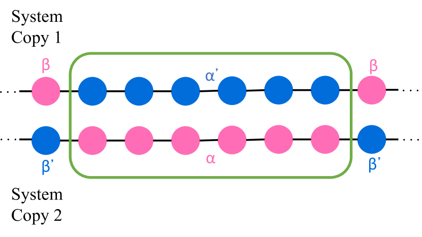
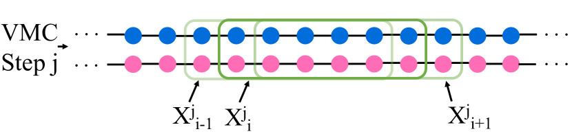
Figure 1: (a) Schematic depiction of the action of the swap operator on a subsystem A. The quantum numbers $\alpha$ describe the subsystem and $\beta$ describe the remainder of the system. Since swap acts on a doubled Hilbert space, we denote the quantum numbers belonging to one copy by primed variables and to the other by unprimed variables. The operator ${\text{{swap}}}_{A}$ switches the primed and unprimed variables within the region A. (b) Illustration of our data collection procedure. At each VMC step $j$, we collect swap data from a collection of subsystems $A_{i}$ and store each in a vector $\vec{X}^{j}$ at index $i$. The collection of $\vec{X}^{j}$’s forms our complete dataset $\mathbf{X}$.

The second step of EntanCl is to project the input data living in the high dimensional space (typically hundreds or thousands of dimensions) down to two-dimensional space in which clustering can be visualized. Typical applications of unsupervised ML to high-dimensional data sets involve visualizing the data in a low-dimensional space via dimensional reduction. Dimensional reduction algorithms (such as those described in refs. Tang et al. (2016); Maaten and Hinton (2008); Coifman and Lafon (2006); Belkin and Niyogi (2002); Tenenbaum et al. (2000); Sammon (1969); Kruskal (1964); Hotelling (1933)) vary in the way that they approximate the high-dimensional manifold populated by the data and what features of that manifold they try to preserve under projection to the low-dimensional space. We are interested in an algorithm that will allow us to visualize the cluster structure in our swap data set $\mathbf{X}$. This is because we expect that those $\vec{X}^{j}$ obtained from groundstateable and non-groundstateable wave functions will appear as two separate clusters due to differing entanglement structure.

We can view clusters from a neighborhood perspective. As an example, in fig. 2 we consider three dimensional data consisting of two clusters: 15 points randomly generated on the upper hemisphere of a unit radius sphere and 15 generated on the lower hemisphere. Gaussian noise is applied to the coordinates of the points. We then project the points down to two dimensions so as to preserve their local neighborhood structure. In this case we use UMAP to do the projection. On the right hand panel of fig. 2, we can see that in each of the two clusters, the local neighborhoods of each point are entirely contained within the same cluster as the point. To emphasize this, we illustrate a local neighborhood of size five around the point marked by a star. From this we can infer that preserving local neighborhood structure also preserves cluster structure. Formally, define a function ${\mathcal{B}^{m}_{\mathbf{X}}}$ such that ${\mathcal{B}^{m}_{\mathbf{X}}}(\vec{X}_{*})\subseteq\mathbf{X}$ is the set of the $m$ nearest neighbors of $\vec{X}_{*}$ in $\mathbf{X}$. A cluster is then a subset $\mathbf{C}\subseteq\mathbf{X}$ such that ${\mathcal{B}^{m}_{\mathbf{X}}}(\vec{C}\in\mathbf{C})\subseteq\mathbf{C}$. For visualizing clusters, a natural choice for a dimensional reduction algorithm is then one that preserves neighborhoods after projection.

Algorithms that preserve neighborhood structure Tang et al. (2016); Maaten and Hinton (2008); Coifman and Lafon (2006); Belkin and Niyogi (2002); Tenenbaum et al. (2000) try to find a mapping $\mathcal{P}$ from the $D$-dimensional data space to $\mathbb{R}^{d}$ (again, $\mathbb{R}^{2}$ for us), such that $\mathcal{P}\circ{\mathcal{B}^{m}_{\mathbf{X}}}=\mathcal{B}^{m}_{\mathbf{\mathcal{P}(X)}}\circ\mathcal{P}$ where $\circ$ denotes the usual composition of mappings. Observe that preserving neighborhoods entails not only keeping points within a cluster nearby, but keeping points in separate clusters far away from each other. Common algorithms accomplish this by taking as input a hyperparameter that defines an estimated neighborhood or cluster size, related to the $m$ in our definition of ${\mathcal{B}^{m}_{\mathbf{X}}}$. These algorithms treat the effective distance between points outside of a neighborhood as extremely (or sometimes infinitely) far away. One must be sure to choose this hyperparameter large enough (based on the density of the data) that spurious clusters do not appear in the projected data. That is to say that the intersection of the neighborhoods ${\mathcal{B}^{m}_{\mathbf{X}}}$ need to contain the entire, true cluster. For our purposes, we use UMAP, which has previously found use in biology Becht et al. (2018); Diaz-Papkovich et al. (2019); Park et al. (2018); Oetjen et al. (2018); Bagger et al. (2018); Clark et al. (2018); Kulkarni et al. (2019); La Manno et al. (2018); Wolf (2018), materials engineering Fuhrimann et al. (2018), and machine learning Blomqvist et al. (2018); Gaujac et al. (2018); Escolano et al. (2018), but has had limited use in quantum matter Li et al. (2019). For more details about how UMAP in particular works, see appendix A. We choose UMAP from the various unsupervised ML algorithms that seek to preserve neighborhood structures for two reasons. Firstly, it led to the most clear projected clustering for our purposes. Secondly, in contrast to other algorithms like tSNE, UMAP provides us with a transferable mapping that can be applied immediately to new data without rerunning UMAP.

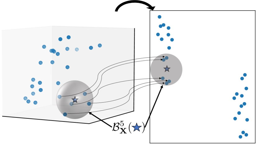
Figure 2: Schematic illustration of ”neighborhood structure” preservation, projecting points in three dimensions to two. The five nearest neighbors of the star are found by application of $\mathcal{B}_{\mathbf{X}}^{5}$. After projection, we can see that the five nearest neighbors of the point marked with a star remain its five nearest neighbors. Moreover, by preserving local neighborhoods, we have discovered two distinct clusters in the high dimensional data. For this example, the projection was done by UMAP.

The final step of EntanCl is to intrepret the learned UMAP output using $k$-means clustering. $K$-means clustering partitions a set of data points into $k$ clusters by placing $k$ cluster means (centroids) in a way that minimizes the sum of squared distances from each data point to its nearest centroid. A $(k=2)$-means clustering thus naturally allows us to classify (non-)groundstateable wave functions in the 2-D projected space. For our test cases where we know which cluster corresponds to each type of wave function, we define a metric of accuracy given by assignment to the correct centroid.

III Band Insulator

To establish EntanCl on a simple, known model, we first study a one-dimensional band insulator. This model is described by the Hamiltonian

$$\mathcal{H}=\sum\limits_{i}(t_{1}b_{i}^{\dagger}a_{i}+t_{2}a^{\dagger}_{i+1}b_{i})+\text{h.c.}.$$ (2)

This model has two bands with energy gap $\Delta E\sim|t_{2}-t_{1}|$, and we consider the case of half filling. We report results in terms of the dimensionless, normalized gap $t\equiv|t_{2}-t_{1}|/t_{1}$. The ground state Slater determinant wave function of the half filled system corresponds to completely filling the lower band. The non-groundstateable eigenstates we consider have some fixed density $n_{ex}\equiv N_{ex}/L$ of randomly chosen $k$-points promoted to the upper band, where $L$ is the system size. This model gives us a testbed to identify ground state wave functions and non-groundstateable wave functions in the parameter space of energy gap $\Delta E$ and excited $k$-point density $n_{ex}$.

The ensemble of swap operators we use in this case is the set of all contiguous length six subsystems of an $L=100$ chain. Our data set $\mathbf{X}$ consists of 1000, 100-dimensional swap vectors $\vec{X}^{j}$ corresponding to the ground state and 1500 corresponding to a non-groundstateable wave function. We choose an uneven ratio of swap data from the two classes to illustrate that a symmetric amount of data is nonessential to our technique. We project the data to two dimensions via UMAP and assign the projected data points to clusters with $k$-means. Since we know which swap data points came from (non-)groundstateable wave functions, we also calculate the accuracy.

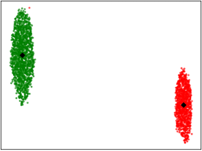
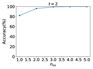
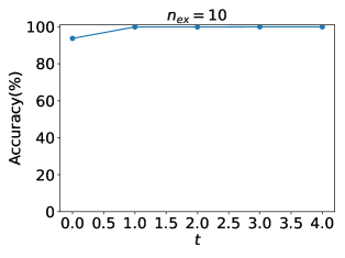
Figure 3: (a) UMAP projection of swap data obtained from wave functions for band insulator model. Red dots correspond to swap data from a groundstateable wave function. Green dots correspond to swap data from a non-groundstateable wave function with $n_{ex}=3\%$ and $t=2$. Black diamonds denote the $(k=2)$-means clustering centroids. This case has accuracy $96.52\%$. We also show the accuracy as a function of (b) excitation density $n_{ex}$ at normalized energy gap $t=2.0$ and (c) $t$ at $n_{ex}=10\%$. In both cases, accuracy increases as a function of the relevant parameter, and moreover, stays relatively high at the minimum possible value.

Our results are shown in figure 3. Fig. 3 (a), corresponds to a projection with the normalized gap $t=2$ and excitation density $n_{ex}=3\%$. In this case one can clearly see the success of EntanCl: the data corresponding to the groundstateable wave function (red) and the non-groundstateable wave function (green) appear as two well separated clusters. This case corresponds to an accuracy of $99.12\%$. In fig. 3(b,c) we can see that as both $t$ and excitation density increase, the accuracy also increases. This makes sense: as both $t$ and $n_{ex}$ increase, the excited state becomes more entangled compared to the ground state as the entanglement entropy scaling transitions from area law to volume law. Moreover, the accuracy stays high even at the lowest possible $n_{ex}$ ($80.00\%$ for $t=2$) and for a gapless system ($90.03\%$ for $n_{ex}=10\%$). This demonstrates that EntanCl is a viable method of identifying the differing entanglement structure in groundstateable and non-groundstateable.

The learned UMAP projection is transferrable. In fig. 4 we illustrate the results of transferring the UMAP projection trained on swap data obtained from the groundstateable wave function and a single non-groundstateable wave function (i.e. single choice of excited $k$-points) with $t=2$ and $n_{ex}=2\%$ to four more non-groundstateable wave functions with the same $t$ and $n_{ex}$. We collect 1000 MC samples for the groundstateable wave function and 1500 for each non-groundstateable wave function. The projection map clusters all the data from non-groundstateable wave functions together, away from the data from the groundstateable wave function. The accuracy in this cas is $84.4\%$, lower than the $96.6\%$ in fig. 3(b) for two wave functions. This is because most of the error is non-groundstateable data being misclassified as groundstateable. Increasing the amount of data collected from the groundstateable wave function would increase the accuracy. These results show that the structure that UMAP is learning generalizes well.

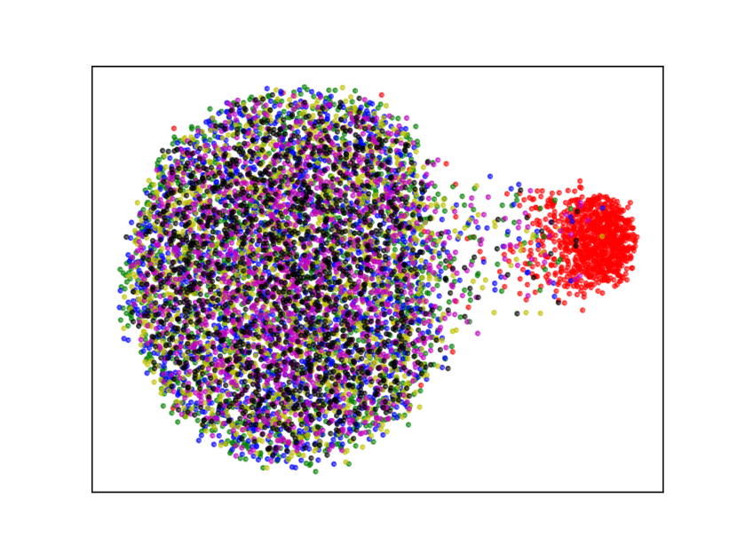
Figure 4: UMAP projection of swap data from band insulator wave functions at gap $t=2$ and excitation density $n_{ex}=2\%$. The UMAP projection was trained using the ground state and a single excited state configuration (i.e. single choice of excited $k$-points). We then transfer the mapping to four more excited state configurations and display the results simultaneously. The ground state data are shown in red, the other colors correspond to various excited state configurations. Clearly, subsequent excited states cluster together with each other, and more importantly all cluster separately from the ground state.

IV Toric Code

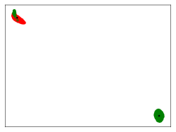
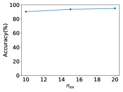
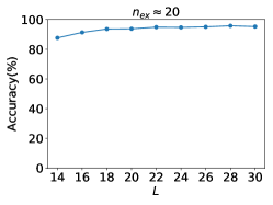
Figure 5: (a) UMAP projection of swap data obtained from wave functions for the toric code. Red dots again correspond to swap data from groundstateable wave functions. Green dots correspond to swap data from a non-groundstateable wave function from a lattice with linear dimension $L=25$ with spinon density $n_{ex}=20\%$. Black diamonds denote the $(k=2)$-means clustering centroids and this case correponds to accuracy $95.91\%$. (b) The accuracy at a fixed lattice size grows with $n_{ex}$, as expected. (c) Classification accuracy for UMAP projection of toric code wave functions as a function of lattice linear dimension. Data shown is at spinon density $\sim 20\%$. Accuracy increases with system size and plateaus around $95\%$. Slight non-monotonicity near the plateau is expected because $n_{ex}$ must be an even integer and is therefore not exactly $20\%$ for all lattice sizes.

We now turn to a two-dimensional example: Kitaev’s toric code Kitaev (2006). This is a strongly interacting system whose ground state has topological order, and because it is exactly solvable, we will be able to assess the accuracy of EntanCl. This model is defined on a square lattice with spin-$1/2$ variables living on the edges. The wave functions that we will consider in this case are eigenstates of the Hamiltonian

$$\mathcal{H} =-\sum\limits_{\square}A_{\square}-\sum\limits_{v}B_{v}$$ (3)

where the operators

$$A_{\square}=\prod\limits_{i\in\square}\sigma^{x}_{i},\ B_{v}=\prod\limits_{i\in\partial v}\sigma^{z}_{i}$$ (4)

are defined as the product of pauli $\sigma^{x}$ operators around a plaquette and $\sigma^{z}$ operators on the edges incident on a vertex $v$ respectively. Note that we will be working in the $\sigma^{z}$ basis.

The ground state wave function we will consider is the equal amplitude superposition of all lattice configurations of closed loops in the trivial homology class. The non-groundstateable wave functions we will consider are equal amplitude superpositions of all states with a fixed spinon density (also allowing closed loops) where a spinon is a vertex $v$ with $B_{v}=-1$. Note that this does not correspond to fixed spinon locations, as such wave functions could be made ground states by simply flipping the sign of the $B_{v}$’s corresponding to the spinon locations. With this model, we will classify wave functions at different values of our control parameter: the spinon density $n_{ex}$.

We collect swap data at 1000 uncorrelated VMC time steps for each wave function we consider. The ensemble of swap operators we use in this case consists of all rectangular subregions of the lattice, which grows with the linear dimension of the lattice $L$ as $L^{4}$. Due to the massively increased dimensionality of the swap data in this case, we add a preprocessing step to compress the data volume for RAM storage, especially for larger system sizes. We average the swap data for a fixed subsystem width and height over all basepoints for the subsystem. This reduces the dimensionality of the data to $L^{2}$, which is sufficiently tractable for our purposes. With this addition to our analysis, we can project the swap data to two dimensions via UMAP.

Our results for the toric code are shown in fig. 5. We find that we can achieve $95.91\%$ accuracy for $n_{ex}=20\%$ for a lattice with linear dimension $L=25$ as shown in fig. 5(a). For a lattice with linear dimension $L=35$ we get accuracy $99.1\%$ even at $n_{ex}=5\%$. Once again, for this high accuracy case, the success of the clustering is remarkably clear. In fig. 5(b), we can see that the accuracy also increases with $n_{ex}$ as we would expect. Moreover, we do not need such a large system to achieve good accuracy. We can see in fig. 5(c) that for $n_{ex}=20\%$, the accuracy of the projection is over $90\%$ already at $L=16$.

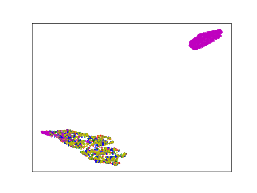
Figure 6: UMAP projection of swap data obtained from the toric code on a $20\times 20$ lattice for all four topologically degenerate ground states and an excited state at excitation density $n_{ex}=20\%$. The projection was trained using only data from the ground state consisting of only homologically trivial loops and the excited state. Then we subsequently apply the projection to the other three ground states. The purple dots are data from the excited state, the other colors are from the ground states. The overall accuracy is $98.04\%$. All of the groundstateable data cluster together and more importantly, cluster separately from the excited state excepting the small fraction of errors.

We now turn to gerneralizability. Due to topological degeneracy, we have access to four groundstateable wave functions from the toric code. In fig. 6 we show the results of training the UMAP projection mapping for a $L=20$ lattice using the groundstateable wave function containing only homologically trivial loops and the non-groundstateable wave function with $n_{ex}=20\%$. We then transfer the projection map to swap data obtained from the other three groundstateable wave functions (those with an odd parity of non-contractible loops around one or both cycles of the torus). In fig. 6, we can see that the data from the non-groundstateable wave function (purple dots) clusters separately from the groundstateable data (other colors), which all clusters together. The accuracy of the collective projection is $98.04\%$, compared to $95.1\%$ from the initial data used to train the projection map. This makes sense because the only errors are non-groundstateable data being classified as groundstateable, so adding more groundstateable data reduces the error. This shows that the learned UMAP projection trained on one ground state generalizes to other ground states in the presence of topological degeneracy.

Another interesting feature of the clustering in this case is that misclassifications are always excited states being incorrectly classified as ground states. The distinction between the ground state and excited state is the presence of spinons and the string operators connecting them. To detect the excited nature of the wave function, a swap operator must swap a subsystem in a way that cuts a string operator. We therefore conjecture that misclassifications of MC samples from excited states as ground states is due to VMC configurations in which the string operators connecting spinons are sufficiently short such that very few subsystems pick up the excited character of the wave function.

V Conclusion

In summary we introduced EntanCl, an unsupervised machine learning method to separate out the ground-stateable wave functions from the exponentially large Hilbert space of many-body wave functions with high computational efficiency. EntanCl consists of three steps: (1) preparation of input data, (2) projection of the data down to two-dimensional space using UMAP, (3) K-means clustering of the projected data. The input data of our choice are matrix elements of an ensemble of swap operators collected as snapshots of individual uncorrelated variational Monte Carlo steps. By using the noisy snapshots as opposed to demanding convergence of the swap operator expectation value, EntanCl gains computational efficiency. We applied EntanCl to a simple one-dimensional band insulator model and from Kitaev’s toric code to find accuracte clustering results. Moreover, we established that the learned UMAP projection is generalizable to an expansion of the data set. The clustering errors are found to occur asymmetrically: an excited state may get misplaced into the ground state cluster but not vice versa. Hence the cluster assignment into excited states will be a reliable way of ruling out groundstateability of the quantum many-body state. As with any VMC sampling, the quality of the results can depend on the sampling basis due to the basis dependence in the spread of the noise. As we demonstrate in appendix B, as long as the spread of the noise remains comparable under a basis transformation, EntanCl will work independent of the basis choice.

In the same vein of addressing wave functions, a more ambitious approach would be to attempt to reconstruct the Hamiltonian that takes a given wave function as its ground state. There has been recent progress in this direction with concrete proposals Qi and Ranard (2019); Bairey et al. (2019); Chertkov and Clark (2018); Garrison and Grover (2018). However, the Hamiltonian reconstruction is computationally costly as it requires precise measurements of many correlation functions. EntanCl can be a swift first pass that can weed out non-groundstateable many-body states without reference to Hamiltonians. Furthermore, as a method that can efficiently sort the swap data associated with different quantum many-body states based on the their entanglement structure, we anticipate EntanCl to find applications beyond separating out ground-stateable wavefunctions. For instance, EntanCl will be ideal for studying quantum phase transitions involving change of entanglement structure due to spontaneous symmetry breaking or topological order Metlitski and Grover (2015).

Acknowledgements: E-AK and MM are supported by the U.S. Department of Energy, Office of Basic Energy Sciences, Division of Materials Science and Engineering under Award DE-SC0018946 Grant. YZ is supported by the startup grant at Peking University. TS is supported by a US Department of Energy grant DE- SC0008739, and in part by a Simons Investigator award from the Simons Foundation. TS is also supported by the Simons Collaboration on Ultra-Quantum Matter, which is a grant from the Simons Foundation (651440, ST).”The project was initiated at Kavli Institute of Theoretical Physics supported by the National Science Foundation under Grant No. NSF PHY-1748958.

Appendix A
Overview of UMAP Procedure

The purpose of the uniform manifold approximation and projection (UMAP) algorithm is to create a low-dimensional projection of high-dimensional data such that the nearest neighbors of a data point in high dimensions remain its nearest neighbors in the low dimensional projection. How many nearest neighbors we try to keep is an input parameter to the algorithm. This is useful for us because data that belong to distinct clusters in the high dimensional space will not share nearest neighbors between clusters. Thus, in the low-dimensional space, these data should still show up as distinct clusters. Here we give an overview of how this algorithm works.

1. Let $X=\{X_{1},\dots,X_{N}\}$ denote our set of input data where each $X_{i}$ is an $n$-dimensional vector. Let $Y=\{Y_{1},\dots,Y_{N}\}$ denote the output projected data points where $Y_{i}$ corresponds to the projection of $X_{i}$ and each $Y_{i}$ is a $d$-dimensional vector with $d\leq n$.

2. We would like the data to be uniformly distributed on the underlying manifold because then the collection of local neighborhoods of our data points provide a good picture of the underlying manifold. UMAP forces our data to be uniformly distributed by normalizing the distance from each point to the furthest neighbor we would like to consider. We are also going to assume that there are no isolated points on the underlying manifold, which we will enforce by fixing the distance to the nearest neighbor. To do this, we define a local metric $d_{i}$ for each input data point $X_{i}$

   $$d_{i}(X_{j},X_{k})=\begin{cases}\frac{1}{r_{i}}d_{\mathbb{R}^{n}}(X_{j},X_{k})-\rho_{i}&\text{if }i=j\text{ or }i=k\\ \infty&\text{otherwise}\end{cases}$$

   where $d_{\mathbb{R}^{n}}$ is the Euclidean metric on $\mathbb{R}^{n}$, $\rho_{i}$ fixes the distance to the nearest neighbor to be zero, and $r_{i}$ fixes the distance to the furthest neighbor we would like to consider. Note that we choose $r_{i}$’s so that for each $d_{i}$, the distance from $X_{i}$ to its furthest relevant neighbor is the same. For the projected output, we will define local metrics as well. The difference in the projected space is that we know what the underlying manifold is ($\mathbb{R}^{d}$) so we know what the true metric is. UMAP still enforces an assumption of local connectivity. Our local metrics for the encoded output $Y_{i}$’s are then

   $$d_{i}(Y_{j},Y_{k})=\begin{cases}d_{\mathbb{R}^{d}}(Y_{j},Y_{k})-\rho_{i}&\text{if }i=j\text{ or }i=k\\ \infty&\text{otherwise}\end{cases}$$

3. Comparisons of distance between our different local metrics are meaningless, which seems to give us no way to assess the quality of a projection. To circumvent this UMAP considers a new represendation of the data: a neighborhood graph. To build the graph, UMAP draws an edge between each data point and each of its neighbors up to the furthest one we would like to consider. The edges are weighted, where for an edge from $X_{i}$ to $X_{j}$, the weight of the edge is $\exp(-d_{i}(X_{i},X_{j}))$. UMAP performs the same procedure for the projected data $Y$. Note that $d_{i}(X_{i},X_{j})$ is not neccesarily equal to $d_{J}(X_{j},X_{i})$. Thus, the edges drawn between $X_{i}$ and $X_{j}$ by $d_{i}$ and $d_{j}$ may not have the same weight.

4. Next UMAP combines edges so that there is at most one edge between any two points. The edges are combined pairwise where for a pair of edges with weights $\alpha,\beta$, UMAP forms a combined edge with weight $f(\alpha,\beta)=\alpha+\beta-\alpha\cdot\beta$. This process occurs for both the input data $X$ and the projected data $Y$. The function $f$ is not the unique way to combine edge weights, but is a choice made by UMAP.

5. Now we have a neighborhood graph for $X$ and $Y$ with an unambiguous definition of the edge between two points. Because the neighborhood graphs for $X$ and $Y$ have the same number of vertices and each vertex is the same degree, we can define an isomorphism between them. We do this by associating projected points with data points being careful to ensure that if there is an edge between $X_{i}$ and $X_{j}$, the points $Y_{i}$ and $Y_{j}$ that we associate with them are also connected by an edge. Thus we can speak unambiguously about a single edge set $E$. To measure the ”similarity” of the two neighborhood graphs, we will use the cross entropy

   $$C(E;\mu_{\cup},\nu_{\cup})\equiv\sum\limits_{e\in E}\mu_{\cup}(e)\log\left(\frac{\mu_{\cup}(e)}{\nu_{\cup}(e)}\right)+$$

   $$(1-\mu_{\cup}(e))\log\left(\frac{1-\mu_{\cup}(e)}{1-\nu_{\cup}(e)}\right)$$

   where $E$ is the set of edges, $\mu_{\cup}(e)$ is the combined weight (as in step 4) of an edge in $Y$, and $\nu_{\cup}(e)$ is the combined weight of an edge in $X$. We can minimize the cross entropy using stochastic gradient descent. For each step of the optimization we move the positions of the encoded points, changing the distance, and therefore the edge weights, between them.

Appendix B
Example of Basis Dependence

A basis transformation can affect the spread in the VMC data obtained during step one of EntanCl by changing the relative magnitudes of the coefficients $C_{\alpha\beta}$ in the wave function (c.f. eq. 1). This change in the spread of the data can affect the accuracy of the resultant clustering if the neighborhoods of MC samples from groundstateable wave functions intersect those of non-groundstateable wave functions in the high dimensional space. Here we discuss an example of the basis dependence of our results by re-examining the band insulator model of section III under a basis transformation. The $k$-space Hamiltonian for the original band insulator model is given by

$$\mathcal{H}_{k}=[t_{1}+t_{2}\cos(k)]\sigma^{x}-t_{2}\sin(k)\sigma^{y}$$ (5)

where the $\sigma^{i}$’s are Pauli matrices. We now consider a new model that differs from the original by an $SU(2)$ unitary transformation with Hamiltonian

$$\mathcal{H}^{\prime} = \sum\limits_{i}t_{1}(a_{i}^{\dagger}a_{i}-b_{i}^{\dagger}b_{i})$$

$$+\frac{t_{2}}{2}(a_{i+1}^{\dagger}a_{i}-b_{i+1}^{\dagger}b_{i}+b_{i+1}^{\dagger}a_{i}-b_{i-1}^{\dagger}a_{i}+\text{h.c.})$$

$$\mathcal{H}_{k}^{\prime}=[t_{1}+t_{2}\cos(k)]\sigma^{z}+t_{2}\sin(k)\sigma^{y}.$$ (7)

This new model $\mathcal{H}_{k}^{\prime}$ describes the same physics as $\mathcal{H}_{k}$, but differs by a basis transformation. We show the clustering accuracy results of scaling the excitation density $n_{ex}$ at fixed normalized gap $t=2$ in fig. 7. We can see that, as was the case in fig. 3, the accuracy is high and remains high even at low $n_{ex}$ values. However, the accuracy in this basis is not as high as in the original basis at the same $n_{ex}$ values. This illustrates that noise in the VMC data does indeed carry a basis dependence, but that sampling data in a new basis does not necessarily destroy the separability of the swap data from groundstateable and non-groundstateable wave functions.

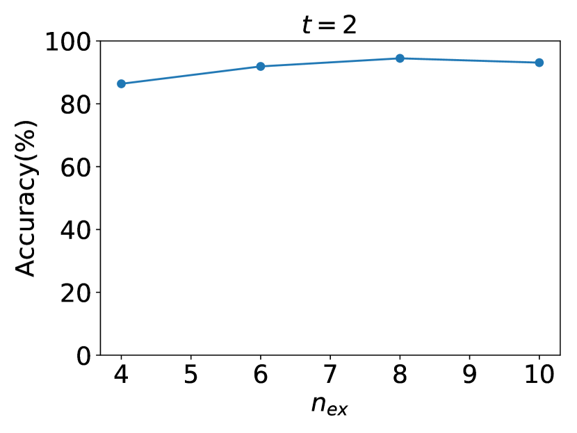
Figure 7: Here we show the clustering accuracy for swap data obtained from the ground state wavefunction of $\mathcal{H}_{k}^{\prime}$ (c.f. eq. 7) and non-groundstateable wave functions with normalized energy gap $t=2$ and varying excitation density $n_{ex}$. Although the accuracy at similar $n_{ex}$ is lower for the model in this basis than the original (c.f. fig. 3(b)), the accuracy is still high (peaking over 90%) and stays above 80% even at low $n_{ex}$ values.

References

- Eisert et al. (2010) J. Eisert, M. Cramer, and M. B. Plenio, Rev. Mod. Phys. 82, 277 (2010).
- Page (1993) D. N. Page, Phys. Rev. Lett. 71, 1291 (1993).
- Foong and Kanno (1994) S. K. Foong and S. Kanno, Phys. Rev. Lett. 72, 1148 (1994).
- Sen (1996) S. Sen, Phys. Rev. Lett. 77, 1 (1996).
- Srednicki (1993) M. Srednicki, Phys. Rev. Lett. 71, 666 (1993).
- Vidmar et al. (2018) L. Vidmar, L. Hackl, E. Bianchi, and M. Rigol, Phys. Rev. Lett. 121, 220602 (2018).
- Vidmar et al. (2017) L. Vidmar, L. Hackl, E. Bianchi, and M. Rigol, Phys. Rev. Lett. 119, 020601 (2017).
- Keating et al. (2015) J. P. Keating, N. Linden, and H. J. Wells, Communications in Mathematical Physics 338, 81 (2015).
- Storms and Singh (2014) M. Storms and R. R. P. Singh, Phys. Rev. E 89, 012125 (2014).
- Ares et al. (2014) F. Ares, J. G. Esteve, F. Falceto, and E. Sánchez-Burillo, Journal of Physics A: Mathematical and Theoretical 47, 245301 (2014).
- Alba et al. (2009) V. Alba, M. Fagotti, and P. Calabrese, Journal of Statistical Mechanics: Theory and Experiment 2009, P10020 (2009).
- Miao and Barthel (2019) Q. Miao and T. Barthel, arXiv preprint arXiv:1905.07760 (2019).
- Broecker et al. (2017a) P. Broecker, J. Carrasquilla, R. G. Melko, and S. Trebst, Scientific Reports 7, 8823 (2017a).
- Broecker et al. (2017b) P. Broecker, F. F. Assaad, and S. Trebst, arXiv preprint (2017b).
- Zhang and Kim (2017) Y. Zhang and E.-A. Kim, Phys. Rev. Lett. 118, 216401 (2017).
- Zhang et al. (2017) Y. Zhang, R. G. Melko, and E.-A. Kim, Phys. Rev. B 96, 245119 (2017).
- Wang (2016) L. Wang, Phys. Rev. B 94, 195105 (2016).
- Carleo and Troyer (2017) G. Carleo and M. Troyer, Science 355, 602 (2017), http://science.sciencemag.org/content/355/6325/602.full.pdf .
- Carrasquilla and Melko (2017) J. Carrasquilla and R. G. Melko, Nature Physics 13, 431 EP (2017).
- van Nieuwenburg et al. (2017) E. P. L. van Nieuwenburg, Y.-H. Liu, and S. D. Huber, Nature Physics 13, 435 EP (2017).
- Beach et al. (2018) M. J. S. Beach, A. Golubeva, and R. G. Melko, Phys. Rev. B 97, 045207 (2018).
- Ch’ng et al. (2017) K. Ch’ng, J. Carrasquilla, R. G. Melko, and E. Khatami, Phys. Rev. X 7, 031038 (2017).
- Ch’ng et al. (2018) K. Ch’ng, N. Vazquez, and E. Khatami, Phys. Rev. E 97, 013306 (2018).
- Deng et al. (2017a) D.-L. Deng, X. Li, and S. Das Sarma, Phys. Rev. B 96, 195145 (2017a).
- Liu and van Nieuwenburg (2018) Y.-H. Liu and E. P. L. van Nieuwenburg, Phys. Rev. Lett. 120, 176401 (2018).
- van Nieuwenburg et al. (2018) E. van Nieuwenburg, E. Bairey, and G. Refael, Phys. Rev. B 98, 060301 (2018).
- Ohtsuki and Ohtsuki (2016) T. Ohtsuki and T. Ohtsuki, Journal of the Physical Society of Japan 85, 123706 (2016), https://doi.org/10.7566/JPSJ.85.123706 .
- Schindler et al. (2017) F. Schindler, N. Regnault, and T. Neupert, Phys. Rev. B 95, 245134 (2017).
- Wetzel and Scherzer (2017) S. J. Wetzel and M. Scherzer, Phys. Rev. B 96, 184410 (2017).
- Wetzel (2017) S. J. Wetzel, Phys. Rev. E 96, 022140 (2017).
- Yoshioka et al. (2018) N. Yoshioka, Y. Akagi, and H. Katsura, Phys. Rev. B 97, 205110 (2018).
- Venderley et al. (2018) J. Venderley, V. Khemani, and E.-A. Kim, Phys. Rev. Lett. 120, 257204 (2018).
- Matty et al. (2019) M. Matty, Y. Zhang, Z. Papic, and E.-A. Kim, arXiv preprint arXiv:1902.04079 (2019).
- Ghosh et al. (2019) S. Ghosh, M. Matty, R. Baumbach, E. D. Bauer, K. Modic, A. Shekhter, J. Mydosh, E.-A. Kim, and B. Ramshaw, arXiv preprint arXiv:1903.00552 (2019).
- Zhang et al. (2018) Y. Zhang, A. Mesaros, K. Fujita, S. Edkins, M. Hamidian, K. Ch’ng, H. Eisaki, S. Uchida, J. Davis, E. Khatami, et al., arXiv preprint arXiv:1808.00479 (2018).
- Cai and Liu (2018) Z. Cai and J. Liu, Phys. Rev. B 97, 035116 (2018).
- Chen et al. (2018) J. Chen, S. Cheng, H. Xie, L. Wang, and T. Xiang, Phys. Rev. B 97, 085104 (2018).
- Deng et al. (2017b) D.-L. Deng, X. Li, and S. Das Sarma, Phys. Rev. X 7, 021021 (2017b).
- Gao and Duan (2017) X. Gao and L.-M. Duan, Nature Communications 8, 662 (2017).
- Huang and Moore (2017) Y. Huang and J. E. Moore, arXiv preprint (2017).
- Liu et al. (2017) J. Liu, Y. Qi, Z. Y. Meng, and L. Fu, Phys. Rev. B 95, 041101 (2017).
- Nomura et al. (2017) Y. Nomura, A. S. Darmawan, Y. Yamaji, and M. Imada, Phys. Rev. B 96, 205152 (2017).
- Schmitt and Heyl (2018) M. Schmitt and M. Heyl, SciPost Phys. 4, 013 (2018).
- Torlai et al. (2018) G. Torlai, G. Mazzola, J. Carrasquilla, M. Troyer, R. Melko, and G. Carleo, Nature Physics 14, 447 (2018).
- McInnes et al. (2018) L. McInnes, J. Healy, and J. Melville, arXiv preprint arXiv:1802.03426 (2018).
- Kitaev (2006) A. Kitaev, Annals of Physics 321, 2 (2006), january Special Issue.
- Hastings et al. (2010) M. B. Hastings, I. González, A. B. Kallin, and R. G. Melko, Phys. Rev. Lett. 104, 157201 (2010).
- Tang et al. (2016) J. Tang, J. Liu, M. Zhang, and Q. Mei, in Proceedings of the 25th international conference on world wide web (International World Wide Web Conferences Steering Committee, 2016) pp. 287–297.
- Maaten and Hinton (2008) L. v. d. Maaten and G. Hinton, Journal of machine learning research 9, 2579 (2008).
- Coifman and Lafon (2006) R. R. Coifman and S. Lafon, Applied and Computational Harmonic Analysis 21, 5 (2006), special Issue: Diffusion Maps and Wavelets.
- Belkin and Niyogi (2002) M. Belkin and P. Niyogi, in Advances in neural information processing systems (2002) pp. 585–591.
- Tenenbaum et al. (2000) J. B. Tenenbaum, V. d. Silva, and J. C. Langford, Science 290, 2319 (2000), https://science.sciencemag.org/content/290/5500/2319.full.pdf .
- Sammon (1969) J. W. Sammon, IEEE Transactions on computers 100, 401 (1969).
- Kruskal (1964) J. B. Kruskal, Psychometrika 29, 1 (1964).
- Hotelling (1933) H. Hotelling, Journal of educational psychology 24, 417 (1933).
- Becht et al. (2018) E. Becht, C.-A. Dutertre, I. W. H. Kwok, L. G. Ng, F. Ginhoux, and E. W. Newell, bioRxiv (2018), 10.1101/298430, https://www.biorxiv.org/content/early/2018/04/10/298430.full.pdf .
- Diaz-Papkovich et al. (2019) A. Diaz-Papkovich, L. Anderson-Trocme, and S. Gravel, bioRxiv , 423632 (2019).
- Park et al. (2018) J.-E. Park, K. Polański, K. Meyer, and S. A. Teichmann, bioRxiv , 397042 (2018).
- Oetjen et al. (2018) K. A. Oetjen, K. E. Lindblad, M. Goswami, G. Gui, P. K. Dagur, C. Lai, L. W. Dillon, J. P. McCoy, and C. S. Hourigan, JCI insight 3 (2018).
- Bagger et al. (2018) F. O. Bagger, S. Kinalis, and N. Rapin, Nucleic acids research 47, D881 (2018).
- Clark et al. (2018) B. Clark, G. Stein-O’Brien, F. Shiau, G. Cannon, E. Davis, T. Sherman, F. Rajaii, R. James-Esposito, R. Gronostajski, E. Fertig, et al., bioRxiv , 378950 (2018).
- Kulkarni et al. (2019) A. Kulkarni, A. G. Anderson, D. P. Merullo, and G. Konopka, Current Opinion in Biotechnology 58, 129 (2019), systems Biology * Nanobiotechnology.
- La Manno et al. (2018) G. La Manno, R. Soldatov, A. Zeisel, E. Braun, H. Hochgerner, V. Petukhov, K. Lidschreiber, M. E. Kastriti, P. Lönnerberg, A. Furlan, J. Fan, L. E. Borm, Z. Liu, D. van Bruggen, J. Guo, X. He, R. Barker, E. Sundström, G. Castelo-Branco, P. Cramer, I. Adameyko, S. Linnarsson, and P. V. Kharchenko, Nature 560, 494 (2018).
- Wolf (2018) W. Wolf, “1. die thematisierung von migration, arbeitsmarkt und nationalstaat,” in Entgrenzungsprozesse in Arbeitsmärkten durch transnationale Arbeitsmigration: World Polity und Nationalstaat im 19. Jahrhundert und heute (Nomos Verlagsgesellschaft mbH & Co. KG, Baden-Baden, 2018) pp. 15–32.
- Fuhrimann et al. (2018) L. Fuhrimann, V. Moosavi, P. O. Ohlbrock, and P. D’acunto, in Proceedings of IASS Annual Symposia, Vol. 2018 (International Association for Shell and Spatial Structures (IASS), 2018) pp. 1–8.
- Blomqvist et al. (2018) K. Blomqvist, S. Kaski, and M. Heinonen, arXiv preprint arXiv:1810.03052 (2018).
- Gaujac et al. (2018) B. Gaujac, I. Feige, and D. Barber, arXiv preprint arXiv:1806.04465 (2018).
- Escolano et al. (2018) C. Escolano, M. R. Costa-jussà, and J. A. Fonollosa, arXiv preprint arXiv:1810.06351 (2018).
- Li et al. (2019) X. Li, O. E. Dyck, M. P. Oxley, A. R. Lupini, L. McInnes, J. Healy, S. Jesse, and S. V. Kalinin, npj Computational Materials 5, 5 (2019).
- Note (1) A loop is a closed, connected path of edges with the same eigenvalue, where at least one vertex that intersects the path has two edges of each eigenvalue incident on it.
- Note (2) Note that in this case all swap matrix elements are either 0 or 1, leading to occasionally redundant . We take only unique here to avoid artificial clusters in the UMAP, but account for the multiplicity in error calculations.
- Qi and Ranard (2019) X.-L. Qi and D. Ranard, Quantum 3, 159 (2019).
- Bairey et al. (2019) E. Bairey, I. Arad, and N. H. Lindner, Phys. Rev. Lett. 122, 020504 (2019).
- Chertkov and Clark (2018) E. Chertkov and B. K. Clark, Phys. Rev. X 8, 031029 (2018).
- Garrison and Grover (2018) J. R. Garrison and T. Grover, Phys. Rev. X 8, 021026 (2018).
- Metlitski and Grover (2015) M. A. Metlitski and T. Grover, arXiv preprint arXiv:1112.5166 (2015).