DoNOF: an open-source implementation of natural-orbital-functional-based methods for quantum chemistry

Abstract

The natural orbital functional theory (NOFT) has emerged as an alternative formalism to both density functional (DF) and wavefunction methods. In NOFT, the electronic structure is described in terms of the natural orbitals (NOs) and their occupation numbers (ONs). The approximate NOFs have proven to be more accurate than those of the density for systems with a significant multiconfigurational character, on one side, and scale better with the number of basis functions than correlated wavefunction methods, on the other side. A challenging task in NOFT is to efficiently perform orbital optimization. In this article we present DoNOF, our open source implementation based on diagonalizations that allows to obtain the resulting orbitals automatically orthogonal. The one-particle reduced-density matrix (1RDM) of the ensemble of pure-spin states provides the proper description of spin multiplets. The capabilities of the code are tested on the water molecule, namely, geometry optimization, natural and canonical representations of molecular orbitals, ionization potential, and electric moments. In DoNOF, the electron-pair-based NOFs developed in our group PNOF5, PNOF7 and PNOF7s are implemented. These $\mathcal{JKL}$-only NOFs take into account most non-dynamic effects plus intrapair-dynamic electron correlation, but lack a significant part of interpair-dynamic correlation. Correlation corrections are estimated by the single-reference NOF-MP2 method that simultaneously calculates static and dynamic electron correlations taking as a reference the Slater determinant formed with the NOs of a previous PNOF calculation. The NOF-MP2 method is used to analyze the potential energy surface (PES) and the binding energy for the symmetric dissociation of the water molecule, and compare it with accurate wavefunction-based methods.

Preprint submitted to Computer Physics Communications

PROGRAM SUMMARY

Program Title: DoNOF: Donostia Natural Orbital Functional Computer Program

Licensing provisions: GNU GPL version 3

Programming language: Fortran

Download: DoNOF can be obtained from the CPC Program Library, and from its public git repository https://github.com/DoNOF/DoNOFsw.

Reference Manual: The DoNOF online manual is available through the link https://donof.readthedocs.io/, from where you can also download it in pdf format.

Nature of problem: Accurate solutions require a balanced treatment of static and dynamic electron correlation. Wavefunction-based methods can handle correctly both types of correlation, however, are computational expensive and demand prior knowledge of the system. Conversely, DF-based methods have a relatively low computational cost. Nowadays, we can find in the literature a wide range of empirical or non-empirical parametrized DFs, however, the list of challenges is still large for DF theory. We need a one-particle formalism more accurate than approximate DFs, but less computationally demanding than wavefunction methods. The answer may be to develop a functional based on the 1RDM. Approximations of the ground-state energy in terms of NOs and their ONs have been developed for practical applications. Minimization of the functional is performed under the orthonormality requirement for the NOs, whereas the ONs conform to the N-representability conditions for the 1RDM. The main challenge is to efficiently perform orbital optimization due to the convergence problems that arise when solving Euler’s nonlinear equations. In addition, the $\mathcal{JKL}$-functionals proposed so far lack a significant part of dynamic correlation, hence correlation corrections must be added to NOF calculations.

Solution method: The DoNOF computer program is designed to solve the energy minimization problem of a NOF that describes the ground-state of an N-electron system at absolute zero temperature. The program includes the NOFs developed in the Donostia quantum chemistry group, namely PNOF5, PNOF7, and PNOF7s. The solution is established by optimizing the energy functional with respect to the ONs and to the NOs, separately. The conjugate gradient or limited memory Broyden-Fletcher-Goldfarb-Shanno (L-BFGS) methods can be employed for the optimization of the ONs. The optimal NOs are obtained by iterative diagonalizations of a symmetric matrix [1] determined by the Lagrange multipliers associated with the orthogonality conditions of NOs. An aufbau principle makes the first-order energy contribution negative upon a diagonalization. To assist convergence, the direct inversion of the iterative subspace (DIIS) extrapolation technique is used, and a variable scale factor balances the symmetric matrix. DoNOF also allows subsequent corrections of the electron correlation once the NOF solution has been obtained. Corrections can be estimated by the single-reference NOF-MP2 method [2] that simultaneously calculates static and dynamic electron correlations taking as a reference the Slater determinant formed with the NOs of the previous PNOF solution. The procedure is simple, showing a formal scaling of $\mathrm{N}_{B}^{5}$ ($\mathrm{N}_{B}$: number of basis functions).

Restrictions: DoNOF is intended for non-relativistic Hamiltonians that does not contain spin coordinates, therefore, our code cannot handle Hamiltonians which break spin symmetry, for example, those that contain a magnetic field term.

Unusual features:

In case of multiplets ($S\neq 0$), our implementation differs from procedures routinely used in electronic structure calculations that focus on the high-spin component or break the spin symmetry. For a given spin $S$, we consider a nondegenerate mixed quantum state that allows all possible $S_{z}$ values.

No prior knowledge of the system is required, so the method can be employed as a black-box. In addition, PNOF is parameter free, so the performance is not subject to specific systems or parametrization data.

Analytic energy gradients with respect to nuclear motion are available in NOFT [3], so the computation of NOF gradients in our code is analogous to gradient calculations at the Hartree-Fock (HF) level of theory. Our implementation allows the calculation of gradients by simple evaluation without resorting to the linear-response theory with the corresponding savings of computational time.

[1] M. Piris, J. M. Ugalde, J. Comput. Chem. 30 (2009) 2078-2086.

[2] M. Piris, Phys. Rev. Lett. 119 (2017) 063002; Phys. Rev. A 98 (2018) 022504.

[3] I. Mitxelena, M. Piris, J. Chem. Phys. 146 (2017) 014102.

I Introduction

Today, computational chemistry helps the experimental chemist understand experimental data, explore reaction mechanisms or predict completely new molecules. There is no doubt that understanding at the molecular level will ultimately lead to an ab initio process design. The best solutions to the many-body problem are offered by methods based on approximate wavefunctions, however, such techniques demand significant computational resources as soon as the systems grow.

It has been known for a long time (Husimi, 1940) that the energy of a system with, at most, two-body interactions is an exact functional of the two-particle reduced density matrix (2RDM). Realistic variational 2RDM calculations are possible nowadays (Mazziotti, 2012a) but they are still computationally expensive. The need for treatments that scale favorably with the number of electrons is evident. The one-particle functional theories, where the ground-state energy is represented in terms of the first-order reduced density matrix (1RDM) (Gilbert, 1975; Valone, 1980) or simply the density (Hohenberg and Kohn, 1964), satisfy this requirement. Unfortunately, computational schemes (Valone, 1991; Mori-Sánchez and Cohen, 2018) based on exact functionals (Levy, 1979; Lieb, 1983) are also expensive, therefore, approximations of the ground-state energy in terms of the density (Burke, 2012; Becke, 2014) or 1RDM (Pernal and Giesbertz, 2016) have been developed for practical applications.

Usually, the local density and generalized gradient approximations are employed for density functionals (DFs), however, they are unable to describe the effects of strong electron correlations. A practical way around this problem has been to use hybrid-exchange functionals, or performing a range separation of the interaction. The resulting functionals appear to work better but the list of failures is still large, for instance, over stabilization of radicals, wrong description of activation barriers, poor treatment of charge transfer processes, and the inability to account for weak interactions (Cohen et al., 2012). Today we have a large number of empirical and non-empirical parameterized functionals, but this large-scale parameterization has led to a very specific applicability in systems and phenomena. For each new challenge, DFs have to be calibrated against the standard wavefunction methods. The last strategy of double hybrid and RPA-based functionals represents a step forward in terms of accuracy, but also leads to a high computational cost.

The key to overcoming these drawbacks may be to ensure the N-repre- sentability (Coleman, 1963), which is twofold in one-particle theories (Piris, 2017a). First, we have the N-representability of the fundamental variable, i.e., the density or 1RDM must come from an N-particle density matrix. Fortunately, conditions to ensure this have been well-established and are easily implementable. Second, approximate functionals must reconstruct the known functional E[2RDM], so the functional N-representability problem arises, that is, we have to meet the requirement that the 2RDM reconstructed in terms of 1RDM or density must satisfy its N-representability conditions as well. Most of the approximate functionals currently-in-use are not N-representable (Ayers and Liu, 2007; Ludeña et al., 2013; Rodríguez-Mayorga et al., 2017). The N-representability constraints for acceptable 1RDM or density are easy to implement, but are insufficient to guarantee that the reconstructed 2RDM is N-representable, and thereby the approximate functional either.

The unknown functional in a 1RDM-based theory only needs to reconstruct the electron-electron potential energy ($V_{ee}$). This reflects an undeniable advantage of 1RDM approximations with respect to approximate DFs which also require a reconstruction of the one-particle term, including the kinetic energy. Our goal is to accomplish a 1RDM formalism more accurate than the approximate DFs, but less computationally demanding than methods based upon approximate wavefunctions or the 2RDM. In 2005 (Piris, 2006), the 2RDM was reconstructed in terms of two-index auxiliary matrices. The latter satisfy the general symmetry properties and sum rules, but also known necessary N-representability conditions of the 2RDM (Piris et al., 2010), namely, the so-called D, Q and G positivity conditions.

In the absence of an external field, the non-relativistic Hamiltonian used in electronic calculations does not contain spin coordinates. Consequently, the ground state of a many-electron system with total spin $S$ is a multiplet, i.e., a mixed quantum state that allows all possible $S_{z}$ values. In this vein, another issue with DFs is that even within the spin-dependent-density formalism they cannot describe the degeneracy of the spin-multiplet components. The proper description of the ensemble of pure spin states is provided by the 1RDM functional theory. In our implementation, the total electronic spin is imposed, not just the spin projection (Piris et al., 2009; Quintero-Monsebaiz et al., 2019; Piris, 2019).

The reconstruction of the 2RDM can be conveniently done in the natural orbital representation where the 1RDM is diagonal. In this spectral representation of the 1RDM, the energy is clearly called natural orbital functional (NOF). A complete account of the formulation and development of NOF theory can be found elsewhere (Piris, 2007). Different ways of approximating the aforementioned auxiliary matrices have led to the appearance of different versions of the Piris NOF (PNOF) (Piris, 2006, 2013; Piris and Ugalde, 2014). Remarkably, the performance of these functionals has achieved chemical accuracy in many cases (Lopez et al., 2010). These functionals are able to yield (Ruipérez et al., 2013) a correct description of systems with a multiconfigurational nature, one of the biggest challenges for DFs.

So far, only the NOFs that satisfy electron pairing restrictions (Piris, 2018a) are able to provide the correct number of electrons in the fragments after a homolytic dissociation (Matxain et al., 2011). For instance, the dissociation curve of the carbon dimer closely resembles that obtained from the optimized CASSCF(8,8) wavefunction (Piris et al., 2016). It has recently been shown (Mitxelena and Piris, 2020a, b) that PNOF7 (Piris, 2017b; Mitxelena et al., 2018) is an efficient method for strongly correlated electrons in one and two dimensions. Our implementation is precisely designed to solve the energy minimization problem of an electron-pairing-based NOF, presented briefly in section II.

The solution is established optimizing the energy functional with respect to the occupation numbers (ONs) and to the natural orbitals (NOs), separately. Under pairing restrictions, the constrained nonlinear programming problem for the ONs can be treated as an unconstrained optimization, with the corresponding saving of computational times. The orbital optimization is the bottleneck of this algorithm since direct minimization of the orbitals has been proved to be a costly method (Cohen and Baerends, 2002; Herbert and Harriman, 2003). In 2009 (Piris and Ugalde, 2009), a self-consistent procedure was proposed which yields the NOs automatically orthogonal. This scheme requires computational times that scale as in the Hartree-Fock (HF) approximation. However, our implementation in the molecular basis set requires also four-index transformation of the electron repulsion integrals (ERIs), which is the time-consuming step, though a parallel implementation of this part of the code substantially improves the performance of our program (Mat, ). To achieve convergence, the direct inversion of the iterative subspace (DIIS) extrapolation technique (Pulay, 1980, 1982) is used, and a variable scale factor balances the symmetric matrix subject to the iterative diagonalizations. In section III, our self-consistent algorithm is introduced, and remarks specific to convergence techniques are discussed. An overview of the DoNOF computational procedure is given at the end of this section.

Section IV is dedicated to molecular properties that can be calculated with DoNOF once the solution is reached. Among these properties are vertical ionization potentials (Piris et al., 2012), Mulliken population analysis (Mulliken, 1955), electric dipole, quadrupole and octupole moments (Mitxelena and Piris, 2016), canonical representation of molecular orbitals (Piris et al., 2013a), analytical energy gradients with respect to nuclear motion (Mitxelena and Piris, 2017), and geometry optimization (Mitxelena et al., 2019). The program also provides RDMs at the atomic and molecular bases, and a wave function file (WFN) to perform additional quantitative and visual analyzes of the molecular systems.

The fact that electron-pairing-based NOFs proposed so far partially lack correlation constitutes their major limitation. They do not fully recover dynamical correlation, which is crucial for the correct description of potential energy surfaces and dispersion interactions. Recently (Piris, 2017b, 2018b, 2019), a new technique that combines the NOF theory with the second-order Møller-Plesset (MP2) perturbation theory was proposed, giving rise to the NOF-MP2 method. The latter is a single-reference method capable of achieving a balanced treatment of static and dynamic electron correlation even for those systems with significant multiconfigurational character. The orbital-invariant formulation of the NOF-MP2 method is briefly presented in section V. The method scales formally as $\mathrm{N}_{B}^{5}$, where $\mathrm{N}_{B}$ is the number of basis functions. The absolute energies improve over PNOF values and get closer to the values obtained by accurate wavefunction-based methods (Piris, 2018b). Likewise, NOF-MP2 is able to give (Lopez and Piris, 2019) a quantitative agreement for dissociation energies, with a performance comparable to that of the accurate CASPT2 method.

In section VI, we show the capabilities of DoNOF for the water molecule as an illustrative example. This includes analysis of molecular orbitals, ionization potential, electric moments, optimized geometry, harmonic vibrational frequencies, binding energy, and potential energy surface of the $H_{2}O$ symmetric dissociation. A summary is given in section VII. Atomic units are used throughout this work.

II Electron-pairing-based NOF for Multiplets

Let us consider a non-relativistic N-electron Hamiltonian that does not contain spin coordinates, namely,

$$\hat{H}=\sum\limits_{ik}\mathcal{H}_{ki}\hat{a}_{k}^{\dagger}\hat{a}_{i}+\frac{1}{2}\sum\limits_{ijkl}\left\langle kl|ij\right\rangle\hat{a}_{k}^{\dagger}\hat{a}_{l}^{\dagger}\hat{a}_{j}\hat{a}_{i}$$ (1)

In Eq. (1), $\mathcal{H}_{ki}$ denote the matrix elements of the one-particle part of the Hamiltonian involving the kinetic energy and the potential energy operators, and $\left\langle kl|ij\right\rangle$ are the two-particle interaction matrix elements. $\hat{a}_{i}^{\dagger}$ and $\hat{a}_{i}$ are the familiar fermion creation and annihilation operators associated with the complete orthonormal spin-orbital set $\left\{\left|i\right\rangle\right\}=\left\{\left|p\sigma\right\rangle\right\}$, where $\sigma$ is used for $\alpha$ and $\beta$ spins. In this context, the ground state with total spin $S$ is a multiplet, i.e., a mixed quantum state (ensemble) that allows all possible spin projections. For a given $S$, there are $\left(2S+1\right)$ energy degenerate eigenvectors $\left|SM_{s}\right\rangle$, so the ground state is defined by the N-particle density matrix statistical operator of all equiprobable pure states:

$$\mathfrak{\hat{D}}={\displaystyle\dfrac{1}{2S+1}{\displaystyle{\textstyle{\displaystyle\sum_{M_{s}=-S}^{S}}}}\left|SM_{s}\right\rangle\left\langle SM_{s}\right|}$$ (2)

From Eq. (1), it follows that the electronic energy is an exactly and explicitly known functional of the RDMs,

$$E=\sum\limits_{ik}\mathcal{H}_{ki}\Gamma_{ki}+\sum\limits_{ijkl}\left\langle kl|ij\right\rangle D_{kl,ij}$$ (3)

where the 1RDM and 2RDM are

$$\begin{array}[]{c}\Gamma_{ki}={\displaystyle\dfrac{1}{2S+1}{\textstyle{\displaystyle\sum_{M_{s}=-S}^{S}}}}\left\langle SM_{s}\right|\hat{a}_{k}^{\dagger}\hat{a}_{i}\left|SM_{s}\right\rangle\\ D_{kl,ij}={\displaystyle{\textstyle{\displaystyle\dfrac{1}{2\left(2S+1\right)}\sum_{M_{s}=-S}^{S}}}}\left\langle SM_{s}\right|\hat{a}_{k}^{\dagger}\hat{a}_{l}^{\dagger}\hat{a}_{j}\hat{a}_{i}\left|SM_{s}\right\rangle\end{array}$$ (4)

We shall use the Löwdin’s normalization, in which the traces of the 1RDM and 2RDM are equal to the number of electrons and the number of electron pairs, respectively.

The first term of Eq. (3) is exactly described as a functional of $\Gamma$, whereas the second is $V_{ee}\left[D\right]$, an explicit functional of the 2RDM. To construct the functional $V_{ee}\left[\Gamma\right]$, we employ the representation where the 1RDM is diagonal ($\Gamma_{ki}=n_{i}\delta_{ki}$). Restriction on the ONs to the range $0\leq n_{i}\leq 1$ represents a necessary and sufficient condition for ensemble N-representability of the 1RDM (Coleman, 1963). This leads to a NOF, namely,

$$E=\sum\limits_{i}n_{i}\mathcal{H}_{ii}+\sum\limits_{ijkl}D[n_{i},n_{j},n_{k},n_{l}]\left\langle kl|ij\right\rangle$$ (5)

In Eq. (5), $D[n_{i},n_{j},n_{k},n_{l}]$ represents the reconstructed ensemble 2RDM from the ONs. For $\hat{S}_{z}$ eigenvectors, density matrix blocks that conserve the number of each spin type are non-vanishing, however, only three of them are independent, namely $D^{\alpha\alpha}$, $D^{\alpha\beta}$, and $D^{\beta\beta}$ (Piris, 2007). In what follows, we briefly describe how we do the reconstruction of $D$ to achieve an electron-pairing-based NOF for spin-multiplets. A more detailed description can be found in Ref. (Piris, 2019).

Let us consider that $\mathrm{N_{I}}$ single electrons determine the spin $S$ of the system, and the rest of electrons ($\mathrm{N_{II}}=\mathrm{N-N_{I}}$) are spin-paired, so that all spins corresponding to $\mathrm{N_{II}}$ electrons provide a zero spin. Obviously, in the absence of single electrons ($\mathrm{N_{I}}=0$), the energy (5) must be reduced to a NOF that describes a singlet state.

We focus on the mixed state of highest multiplicity: $2S+1=\mathrm{N_{I}}+1,\,S=\mathrm{N_{I}}/2$. Then, the expected value of $\hat{S}_{z}$ for the whole ensemble $\left\{\left|SM_{s}\right\rangle\right\}$ is zero, namely,

$$\mathrm{<}\hat{S}_{z}\mathrm{>}=\frac{1}{\mathrm{N_{I}}+1}{\textstyle{\displaystyle\sum_{M_{s}=-\mathrm{N_{I}}/2}^{\mathrm{N_{I}}/2}}M_{s}}=0$$ (6)

According to Eq. (6), we can adopt the spin-restricted theory in which a single set of orbitals $\left\{\left|p\right\rangle\right\}$ is used for $\alpha$ and $\beta$ spins. All spatial orbitals will be then double occupied in the ensemble, so that occupancies for particles with $\alpha$ and $\beta$ spins are equal: $n_{p}^{\alpha}=n_{p}^{\beta}=n_{p}.$

In turn let us divide the orbital space $\Omega$ into two subspaces: $\Omega=\Omega_{\mathrm{I}}\oplus\Omega_{\mathrm{II}}$. $\Omega_{\mathrm{II}}$ is composed of $\mathrm{N_{II}}/2$ mutually disjoint subspaces $\Omega{}_{g}$. Each subspace $\Omega{}_{g}\in\Omega_{\mathrm{II}}$ contains one orbital $\left|g\right\rangle$ with $g\leq\mathrm{N_{II}}/2$, and $\mathrm{N}_{g}$ orbitals $\left|p\right\rangle$ with $p>\mathrm{N_{II}}/2$, namely,

$$\Omega{}_{g}=\left\{\left|g\right\rangle,\left|p_{1}\right\rangle,\left|p_{2}\right\rangle,...,\left|p_{\mathrm{N}_{g}}\right\rangle\right\}$$ (7)

Taking into account the spin, the total occupancy for a given subspace $\Omega{}_{g}$ is 2, which is reflected in the following sum rule:

$$n_{g}+\sum_{i=1}^{\mathrm{N}_{g}}n_{p_{i}}=1,\quad g=1,2,...,\frac{\mathrm{N_{II}}}{2}$$ (8)

In general, $\mathrm{N}_{g}$ may be different for each subspace, but it should be sufficient for the description of each electron pair. In our implementation, $\mathrm{N}_{g}$ is equal to a fixed number for all subspaces $\Omega{}_{g}\in\Omega_{\mathrm{II}}$. The maximum possible value of $\mathrm{N}_{g}$ is determined by the basis set used in calculations.

From (8), it follows that

$$2\sum_{p\in\Omega_{\mathrm{II}}}n_{p}=2\sum_{g=1}^{\frac{\mathrm{N_{II}}}{2}}\left(n_{g}+\sum_{i=1}^{\mathrm{N}_{g}}n_{p_{i}}\right)=\mathrm{N_{II}}$$ (9)

Here, the notation $p\in\Omega_{\mathrm{II}}$ represents all the indexes of $\left|p\right\rangle$ orbitals belonging to $\Omega_{\mathrm{II}}$. It is important to recall that orbitals belonging to each subspace $\Omega_{g}$ vary along the optimization process until the most favorable orbital interactions are found. Therefore, the orbitals do not remain fixed in the optimization process, they adapt to the problem.

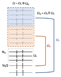
Figure 1: Splitting of the orbital space $\Omega$ into subspaces. In this example, $S=3/2$ (quartet) and $\mathrm{N_{I}}=3$, so three orbitals make up the subspace $\Omega_{\mathrm{I}}$, whereas four electrons ($\mathrm{N_{II}}=4$) distributed in two subspaces $\left\{\Omega_{1},\Omega_{2}\right\}$ make up the subspace $\Omega_{\mathrm{II}}$. Note that $\mathrm{N}_{g}=4$. The arrows depict the values of the ensemble occupation numbers, alpha ($\downarrow$) or beta ($\uparrow$), in each orbital.

Similarly, $\Omega_{\mathrm{I}}$ is composed of $\mathrm{N_{I}}$ mutually disjoint subspaces $\Omega{}_{g}$. In contrast to $\Omega_{\mathrm{II}}$, each subspace $\Omega{}_{g}\in\Omega_{\mathrm{I}}$ contains only one orbital $g$ with $2n_{g}=1$. It is worth noting that each orbital is completely occupied individually, but we do not know whether the electron has $\alpha$ or $\beta$ spin: $n_{g}^{\alpha}=n_{g}^{\beta}=n_{g}=1/2$. It follows that

$$2\sum_{p\in\Omega_{\mathrm{I}}}n_{p}=2\sum_{g=\frac{\mathrm{N_{II}}}{2}+1}^{\mathrm{N}_{\Omega}}n_{g}=\mathrm{N_{I}},$$ (10)

where $\mathrm{\mathrm{N}_{\Omega}=}\mathrm{N_{II}}/2+\mathrm{N_{I}}$ denotes the total number of subspaces in $\Omega$. Taking into account Eq. (9), the trace of the 1RDM is verified equal to the number of electrons:

$$2\sum_{p\in\Omega}n_{p}=2\sum_{p\in\Omega_{\mathrm{II}}}n_{p}+2\sum_{p\in\Omega_{\mathrm{I}}}n_{p}=\mathrm{N_{II}}+\mathrm{N_{I}}=\mathrm{\mathrm{N}}$$ (11)

In Fig. 1, an illustrative example is shown. In this example, $\mathrm{N_{I}}=3$ ($S=3/2$) hence three orbitals make up the subspace $\Omega_{\mathrm{I}}$, whereas four electrons ($\mathrm{N_{II}}=4$) distributed in two subspaces $\left\{\Omega_{1},\Omega_{2}\right\}$ make up the subspace $\Omega_{\mathrm{II}}$. In Fig. 1, $\mathrm{N}_{g}=4$ corresponds to the maximum allowed value.

In DoNOF, we employ a two-index reconstruction $D[n_{p},n_{q}]$ (Piris, 2006), instead of the general dependence on four indices. The necessary N-representability D, Q, and G conditions of the 2RDM, also known as (2,2)-positivity conditions (Mazziotti, 2012b), impose strict inequalities on $D$-elements (Piris et al., 2010). Given these constraints, some proposals have resulted in several $\mathcal{JKL}$-only functionals (Piris, 2013), where $\mathcal{J}$ and $\mathcal{K}$ refer to the usual Coulomb and exchange integrals, while $\mathcal{L}$ denotes the exchange-time-inversion integral (Piris, 1999).

For an electron-pairing-based NOF, we divide the matrix elements of $D$ into intra- and inter-subspace contributions. The intra-subspace blocks only involves intrapair $\alpha\beta$-contributions of orbitals belonging to $\Omega_{\mathrm{II}}$. Actually, there can be no interactions between electrons with opposite spins in a singly occupied orbital, since there is only one electron with $\alpha$ or $\beta$ spin in each $\left|SM\right\rangle$ of the ensemble. In the simplest case of two electrons, an accurate NOF is well-known from the exact wavefunction Lowdin and Shull (1955). Consequently, the intrapair $\alpha\beta$-contributions are

$$\begin{array}[]{c}D_{pq,rt}^{\alpha\beta}={\displaystyle\frac{\Pi_{pr}}{2}}\delta_{pq}\delta_{rt}\delta_{p\Omega_{g}}\delta_{r\Omega_{g}}\;(g\leq\frac{N_{\mathrm{II}}}{2})\\ \\ \Pi_{pr}=\left\{\begin{array}[]{c}\sqrt{n_{p}n_{r}}\qquad p=r\textrm{ or }p,r>\frac{N_{\mathrm{II}}}{2}\\ -\sqrt{n_{p}n_{r}}\qquad p=g\textrm{ or }r=g\end{array}\right.\\ \\ \delta_{p\Omega_{g}}=\left\{\begin{array}[]{c}1\qquad p\in\Omega_{g}\in\Omega_{\mathrm{II}}\\ 0\qquad p\notin\Omega_{g}\in\Omega_{\mathrm{II}}\end{array}\right.\end{array}$$ (12)

Note that $D_{pp,pp}^{\alpha\beta}=0$, $\forall p\in\Omega_{\mathrm{I}}$. For inter-subspace contributions ($\Omega_{f}\neq\Omega{}_{g}$), the spin-parallel matrix elements are HF like, namely,

$$D_{pq,rt}^{\sigma\sigma}={\displaystyle\frac{n_{p}n_{q}}{2}}\left(\delta_{pr}\delta_{qt}-\delta_{pt}\delta_{qr}\right)\delta_{p\Omega_{f}}\delta_{q\Omega_{g}},\>{}_{\sigma=\alpha,\beta}$$ (13)

whereas the spin-anti-parallel blocks are

$$\begin{array}[]{c}D_{pq,rt}^{\alpha\beta}={\displaystyle{\displaystyle\frac{n_{p}n_{q}}{2}}}\delta_{pr}\delta_{qt}\delta_{p\Omega_{f}}\delta_{q\Omega_{g}}-{\displaystyle\frac{\Phi_{p}\Phi_{r}}{2}}\delta_{p\Omega_{f}}\delta_{r\Omega_{g}}\cdot\\ \\ \cdot\left\{\begin{array}[]{c}\delta_{pq}\delta_{rt}\quad f\leq\frac{\mathrm{N_{II}}}{2}\textrm{ or }g\leq\frac{\mathrm{N_{II}}}{2}\\ \quad\delta_{pt}\delta_{qr}\qquad\frac{\mathrm{N_{II}}}{2}<f,g\leq\mathrm{N}_{\Omega}\end{array}\right.\end{array}$$ (14)

where $\Phi_{p}=\sqrt{n_{p}(1-n_{p})}$. It is not difficult to verify (Piris, 2019) that the reconstruction (12)-(14) leads to $\mathrm{<}\hat{S}^{2}\mathrm{>}=S\left(S+1\right)$ with $S=\mathrm{N_{I}}/2$.

In quantum chemistry, we usually use real spatial orbitals, then $\mathcal{L}_{pq}=\mathcal{K}_{pq}$. After a simple algebra, the energy (5) can be written as

$$E=\sum\limits_{g=1}^{\frac{\mathrm{N_{II}}}{2}}E_{g}+\sum_{g=\frac{\mathrm{N_{II}}}{2}+1}^{\mathrm{N}_{\Omega}}\mathcal{H}_{gg}+\sum\limits_{f,g=1;f\neq g}^{\mathrm{N}_{\Omega}}E_{fg}$$ (15)

where

$$E_{g}=2\sum\limits_{p\in\Omega_{g}}n_{p}\mathcal{H}_{pp}+\sum\limits_{q,p\in\Omega_{g}}\Pi_{qp}\mathcal{K}_{pq}\,,\;\Omega{}_{g}\in\Omega_{\mathrm{II}}$$ (16)

is the energy of an electron pair with opposite spins. $E_{fg}$ correlates the motion of electrons with parallel and opposite spins belonging to different subspaces ($\Omega_{f}\neq\Omega{}_{g}$):

$$E_{fg}=\sum\limits_{p\in\Omega_{f}}\sum\limits_{q\in\Omega_{g}}\left[n_{q}n_{p}\left(2\mathcal{J}_{pq}-\mathcal{K}_{pq}\right)-\Phi_{q}\Phi_{p}\mathcal{K}_{pq}\right]$$ (17)

The functional (15)-(17) is PNOF7 for multiplets (Piris, 2017b; Mitxelena et al., 2018; Piris, 2018b). It is worth noting that PNOF7 is reduced to PNOF5 (Piris et al., 2011, 2013b) for $\Phi_{p}\equiv 0$. The latter constitutes an independent-pair approximation by not considering the interaction between orbitals that belong to different subspaces beyond the HF terms of Eq. (17). It will afford good results when the number of electron pairs is small, but the results deteriorate rapidly as the system grows. Interestingly, an antisymmetrized product of strongly orthogonal geminals (APSG) with the expansion coefficients explicitly expressed by the ONs also leads to PNOF5 (Piris et al., 2013b) showing that PNOF5 is strictly N-representable. As far as we know, there is no other NOF for which its generating wavefunction is known.

PNOF7 introduces interaction terms between orbitals belonging to different subspaces. Its main weakness is the absence of the dynamic electron correlation between pairs, since $\Phi_{p}=\sqrt{n_{p}(1-n_{p})}$ has significant values only when the ONs differ substantially from 1 and 0. Consequently, PNOF7 is able to recover the complete intrapair, but only the static interpair correlation. The functional has proven its worth in problems where a strong correlation is revealed. We have recently demonstrated (Mitxelena and Piris, 2020a, b) the ability of PNOF7 to describe strong correlation effects in one-dimensional and two-dimensional systems by comparing our results with exact diagonalization, density matrix renormalization group, and quantum Monte Carlo calculations. Unfortunately, PNOF7 does not include dynamic interpair correlation, which can be included a posteriori using a modified version of standard second-order perturbation theory (see below in section V).

III Energy minimization problem

Minimization of the energy functional $E\left[\mathrm{N},\left\{n_{p}\right\},\left\{\varphi_{p}\left(\mathbf{r}\right)\right\}\right]$ is performed under the orthonormality requirement for the real spatial orbitals,

$$\left\langle p|q\right\rangle=\int d\mathbf{r}\varphi_{p}\left(\mathbf{r}\right)\varphi_{q}\left(\mathbf{r}\right)=\delta_{pq}$$ (18)

whereas the occupancies conform to the ensemble N-representability conditions $0\leq n_{p}\leq 1$, and pairing sum rules (8). The latter are important for orbitals belonging to $\Omega_{\mathrm{II}}$ since $n_{p}=1/2$, $\forall p\in\Omega_{\mathrm{I}}$. This is a constrained optimization problem. The solution is established by optimizing the energy (15) with respect to the ONs and to the NOs, separately.

III.1 Occupancy Optimization

Bounds on $\left\{n_{p}\right\}$ can be imposed automatically by expressing the ONs through new auxiliary variables $\left\{\gamma_{p}\right\}$, and using trigonometric functions. Likewise, the equality constrains (8) can also always be satisfied using the properties of these functions. In this way, we transform the constrained minimization problem of the objective function with respect to $\left\{n_{p}\right\}$ into the problem of minimizing $E$ with respect to auxiliary variables $\left\{\gamma_{p}\right\}$ without restrictions on their values. In our implementation, the conjugate gradient (CG) method (Fletcher, 2000) is used for performing the optimization of the energy with respect to $\gamma$-variables.

Let us set the ON of an orbital $\left|g\right\rangle$ as

$$n_{g}=\dfrac{1}{2}\left(1+cos^{2}\gamma_{g}\right);\>g=1,2,...,\mathrm{N_{II}}/2$$ (19)

Given the range $[0,1]$ of possible values for $cos^{2}\gamma_{g}$, it is easy to see that $1/2\leq n_{g}\leq 1$. Accordingly, we shall name $\left\{\varphi_{g}\left(\mathbf{r}\right);g=1,2,...,N_{\mathrm{II}}/2\right\}$ strongly occupied orbitals. The pairing conditions (8) can be conveniently written as

$$\sum_{i=1}^{\mathrm{N}_{g}}n_{p_{i}}=h_{g};\quad g=1,2,...,\mathrm{N_{II}}/2$$ (20)

where the hole $h_{g}=1-n_{g}$ in the orbital $\left|g\right\rangle$ is $h_{g}=\left(sin^{2}\gamma_{g}\right)/2$. Let us express the ONs of the rest of orbitals through new auxiliary variables while satisfying Eq. (20). Indeed, the ONs $\left\{n_{p_{1}},n_{p_{2}},...,n_{p_{\mathrm{N}_{g}}}\right\}$ of each subspace $\Omega{}_{g}\in\Omega_{\mathrm{II}}$ can be set as

$$\begin{array}[]{c}n_{p_{1}}=h_{g}sin^{2}\gamma_{p_{1}}\\ \\ n_{p_{2}}=h_{g}cos^{2}\gamma_{p_{1}}sin^{2}\gamma_{p_{2}}\\ \\ \cdots\\ \\ n_{p_{i}}=h_{g}cos^{2}\gamma_{p_{1}}cos^{2}\gamma_{p_{2}}\cdots cos^{2}\gamma_{p_{i-1}}sin^{2}\gamma_{p_{i}}\\ \\ \cdots\\ \\ n_{p_{\mathrm{N}_{g}-1}}=h_{g}cos^{2}\gamma_{p_{1}}cos^{2}\gamma_{p_{2}}\cdots cos^{2}\gamma_{p_{\mathrm{N}_{g}-2}}sin^{2}\gamma_{p_{\mathrm{N}_{g}-1}}\\ \\ n_{p_{\mathrm{N}_{g}}}=h_{g}cos^{2}\gamma_{p_{1}}cos^{2}\gamma_{p_{2}}\cdots cos^{2}\gamma_{p_{\mathrm{N}_{g}-2}}cos{}^{2}\gamma_{p_{\mathrm{N}_{g}-1}}\\ \\ \end{array}$$ (21)

It is not difficult to verify if we add the equations of (21) in pairs, starting with the last two and continuing upwards using the resulting equation of each sum, that the restriction (20) is always fulfilled thanks to the fundamental trigonometric identity. Note that by eliminating the equality restrictions (20) from the problem, we move from having $\mathrm{N}_{g}$ unknown occupancies to $\mathrm{N}_{g}-1$ auxiliary $\gamma$-variables. Finally, taking into account that $sin^{2}\left(\gamma\right)$ and $cos^{2}\left(\gamma\right)$ are always in the interval $[0,1]$, and that these multiply the magnitude of the hole $h_{g}$, the rest of orbitals in $\Omega_{\mathrm{II}}$ are weakly occupied, i.e., $0\leq n_{p}\leq 1/2$ if $p>\mathrm{N_{II}}/2\cap p\in\Omega_{\mathrm{II}}$.

III.2 Orbital Optimization

The orthonormal conditions may be taken into account by the Lagrange multiplier method. For a fixed set of occupancies, let us introduce the symmetric multipliers $\left\{\lambda_{pq}\right\}$ associated with orthonormality constraints (18) on the real spatial orbitals $\left|p\right\rangle$, and define the auxiliary functional $\Omega$ as

$$\Omega=E-2{\displaystyle\sum_{pq}}\lambda_{qp}\left(\left\langle p|q\right\rangle-\delta_{pq}\right)$$ (22)

The functional (22) has to be stationary with respect to variations in $\varphi_{p}\left(\mathbf{r}\right)$, that is

$$\delta\Omega=\sum\limits_{p}\int d\mathbf{r}\delta\varphi_{p}\left(\mathbf{r}\right)\left[\frac{\delta E}{\delta\varphi_{p}\left(\mathbf{r}\right)}-{\displaystyle 4\sum_{q}}\lambda_{qp}\varphi_{q}\left(\mathbf{r}\right)\right]=0$$ (23)

which leads to the following orbital Euler equations

$$\frac{\delta E}{\delta\varphi_{p}\left(\mathbf{r}\right)}=4n_{p}\mathcal{\hat{H}}\varphi_{p}\left(\mathbf{r}\right)+\frac{\delta V_{ee}}{\delta\varphi_{p}\left(\mathbf{r}\right)}={\displaystyle 4\sum_{q}}\lambda_{qp}\varphi_{q}\left(\mathbf{r}\right)$$ (24)

The functional derivative of $V_{ee}$ with respect to $\varphi_{p}$ at the point $\mathbf{r}$ depends on the subspace $\Omega{}_{g}$ to which the orbital belongs. For orbitals belonging to a subspace with a single electron ($\varphi_{p}\in\Omega{}_{g}\in\Omega_{\mathrm{I}}$) only inter-pair contributions appear, and the functional derivative is given by the following expression

$$\begin{array}[]{c}{\displaystyle\frac{\delta V_{ee}^{inter}}{\delta\varphi_{p}\left(\mathbf{r}\right)}}=4\left\{\sum\limits_{f=1;f\neq g}^{\mathrm{N}_{\Omega}}\sum\limits_{q\in\Omega_{f}}\left[n_{q}n_{p}\left(2\mathcal{\hat{J}}_{q}-\hat{\mathcal{K}}_{q}\right)\right.\right.\\ \\ \left.\left.-\Phi_{q}\Phi_{p}\hat{\mathcal{K}}_{q}\right]\right\}\varphi_{p}\left(\mathbf{r}\right)\end{array}$$ (25)

where

$$\mathcal{\hat{J}}_{q}\left(\mathbf{r}\right)=\int d\mathbf{r}^{\prime}\frac{\;\left|\varphi_{q}\left(\mathbf{r}^{\prime}\right)\right|^{2}}{\left|\mathbf{\mathbf{r}-r}^{\prime}\right|}$$ (26)

$$\hat{\mathcal{K}}_{q}\left(\mathbf{r}\right)=\int d\mathbf{r}^{\prime}\varphi_{q}\left(\mathbf{r}^{\prime}\right)\frac{\hat{P}_{\mathbf{r},\mathbf{r}^{\prime}}}{\left|\mathbf{\mathbf{r}-r}^{\prime}\right|}\varphi_{q}\left(\mathbf{r}^{\prime}\right)$$ (27)

are the usual Coulomb and exchange operators, respectively, and $\hat{P}_{\mathbf{r},\mathbf{r}^{\prime}}$ is the permutation operator. For orbitals belonging to a subspace with an electron pair we must also include the intrapair contribution,

$$\frac{\delta V_{ee}}{\delta\varphi_{p}\left(\mathbf{r}\right)}=\frac{\delta V_{ee}^{inter}}{\delta\varphi_{p}\left(\mathbf{r}\right)}+4\sum\limits_{q\in\Omega_{g}}\Pi_{qp}\mathcal{\hat{K}}_{q}\varphi_{p}\left(\mathbf{r}\right);\>\varphi_{p}\in\Omega{}_{g}\in\Omega_{\mathrm{II}}$$ (28)

The functional (22) must also be stationary with respect to variations in Lagrange multipliers, which leads to the Eqs. (18). For a fixed set of ONs, we have to find $\left\{\varphi_{p}\right\}$ and $\left\{\lambda_{qp}\right\}$ that solve Eqs. (18) and (24). In general, the energy functional of Eq. (15) is not invariant with respect to an orthogonal transformation of the orbitals. Consequently, Eq. (24) cannot be reduced to a pseudo-eigenvalue problem by diagonalizing the $\mathbf{\lambda}$ matrix. This system of equations is nonlinear in $\varphi_{p}$ so it is formidable to solve, although the symmetry property of $\mathbf{\lambda}$ may be used to simplify the problem. In our implementation, we employ the self-consistent procedure proposed in (Piris and Ugalde, 2009) to obtain the NOs.

Multiplying the Eq. (24) by $\varphi_{p}$, integrating over $\mathbf{r}$, and taking into account the Eq. (18), we get

$$\lambda_{qp}=n_{p}\mathcal{H}_{qp}+g_{pq}$$ (29)

where

$$g_{pq}=\int d\mathbf{r}\frac{\delta V_{ee}}{\delta\varphi_{p}\left(\mathbf{r}\right)}\varphi_{q}\left(\mathbf{r}\right)$$ (30)

At the extremum, the matrix of the Lagrange multipliers must be a symmetric matrix : $\lambda_{qp}=\lambda_{pq}$. Considering $\lambda_{qp}-\lambda_{pq}$, and that $\mathcal{H}$ is a symmetric matrix, it follows without difficulty that

$$\left(n_{p}-n_{q}\right)\mathcal{H}_{qp}+g_{pq}-g_{qp}=0$$ (31)

Eq. (31) eliminates the Lagrange multipliers as variables in the problem, that is, the original Eqs. have been replaced by the system of Eqs. (31) and (18) over the unknown $\varphi_{p}$ functions only. Introducing a set of known basis functions, the integral differential Eqs. (31) can be cast into an algebraic equations, however, the standard methods for solving this nonlinear system of Eqs. converge very slowly.

Let us define the off-diagonal elements of a symmetric matrix $\mathcal{F}$ as

$$\mathcal{F}_{qp}=\theta\left(p-q\right)[\lambda_{qp}-\lambda_{pq}]+\theta\left(q-p\right)[\lambda_{pq}-\lambda_{qp}]$$ (32)

where $\theta\left(x\right)$ is the unit-step Heaviside function. According to Eq. (31), $\mathcal{F}_{qp}$ vanishes at the extremum, hence matrices $\mathcal{F}$ and $\Gamma$ can be brought simultaneously to a diagonal form at the solution. Hence, $\varphi_{p}$’s which solve the Eqs. (31), may be accomplished by diagonalization of the matrix $\mathcal{F}$ in an iterative way. A remarkable advantage of this procedure is that the orthonormality constraints (18) are automatically guaranteed. Unfortunately, the diagonal elements cannot be determined from the symmetry property of $\mathbf{\lambda}$, so this procedure does not provide a generalized Fockian in the conventional sense. Nevertheless, $\lambda_{pp}$ may be determined with the help of an aufbau principle.

Let us consider an almost diagonal matrix $\mathcal{F}^{0}$ constructed from the set of orbitals $\left\{\varphi_{p}^{0}\right\}$ according to Eq. (32) with diagonal elements $\mathcal{F}_{pp}^{0}$, and let $E^{0}$ be the corresponding electronic energy. Up to the first-order terms, the diagonalization of $\mathcal{F}^{0}$ gives rise to a new set of orbitals (Saunders and Hillier, 1973),

$$\varphi_{p}=\varphi_{p}^{0}+\sum_{q,q\neq p}\frac{\mathcal{F}_{qp}^{0}\varphi_{q}^{0}}{\mathcal{F}_{pp}^{0}-\mathcal{F}_{qq}^{0}}$$ (33)

The first-order expression for the energy corresponding to the orbitals defined in Eq. (33) reads

$$E=E^{0}+2\sum_{p<q}\frac{\left|\mathcal{F}_{pq}^{0}\right|^{2}}{\mathcal{F}_{pp}^{0}-\mathcal{F}_{qq}^{0}}$$ (34)

It is clear from Eq. (34) that if we choose $\mathcal{F}_{qq}^{0}>\mathcal{F}_{pp}^{0}$, making the first-order energy contribution negative, the energy is bound to drop upon the diagonalization of $\mathcal{F}^{0}$. Consequently, NOs may be attained by iterative diagonalization of matrix $\mathcal{F}$ employing the above aufbau principle for the definition of the diagonal elements.

In DoNOF, we maintain the values of the previous diagonalization of $\mathcal{F}$ to use them as diagonal elements in each step. Different $\mathcal{F}$ matrices may come out depending on the initial guess. In the absence of static correlation, a good start for $\left\{\mathcal{F}_{pp}^{0}\right\}$ is usually the values obtained after an energy optimization with respect to $\gamma$ and a single diagonalization of the symmetrized $\lambda$-matrix, $\left(\lambda_{pq}+\lambda_{qp}\right)/2$, calculated with the HF orbitals. If static correlation plays an important role, it is generally a better option to replace the HF orbitals with the eigenvectors of the one-particle part of the Hamiltonian ($\mathcal{H}$).

From Eq. (34), it can be seen that the off-diagonal elements must be small enough, so that each element $\mathcal{F}_{pq}$ communicates its appropriate significance in each step of the iterative diagonalization process. Accordingly, a well-scaled $\mathcal{F}$ matrix turns crucial in order to decrease the energy. In our implementation, the scaling of $\mathcal{F}$ is achieved by dividing those elements $\mathcal{F}_{pq}$ that exceed some small value $\zeta$ several times by ten, so that the value of each matrix element results of the same order of magnitude and lesser than the upper selected bound $\zeta$.

It is important to note that the orbitals belonging to different subspaces vary throughout the optimization process until the most favorable orbital interactions are found, that is, there is no impediment to mixing orbitals from the different subspaces to arrive at the optimal orbitals. Consequently, the orbital optimization procedure is independent of the selected initial orbital coupling, although a proper initial guess favors a faster convergence of this procedure.

III.3 Convergence Acceleration

It is well-known that iterative methods frequently suffer from slow convergence. To accelerate convergence we have implemented a DIIS extrapolation technique (Pulay, 1980). In the latter, an error vector $\mathbf{e}^{j}$ is constructed at each $j$th step. The construction of a suitable error vector is related to the gradient of the electronic energy with respect to $\varphi$ and thus vanishes for the solution. In DoNOF, we use the off-diagonal elements of the symmetric matrix $\mathcal{F}$ given by Eq. (32) to form the error vector, namely, $e_{pq}^{j}=\mathcal{F}_{pq}^{j}$ (recall that $\mathcal{F}_{pq}\rightarrow 0$ at the converged solution).

Toward the end of the iterative procedure, changes in $\varphi$ are small and it is possible to find a linear combination of $m$ consecutive error vectors that approximates the zero vector in the least-squares sense:

$$\Delta\mathbf{e}=\sum_{j=1}^{m}c_{j}\mathbf{e}^{j}\rightarrow 0$$ (35)

where the coupling constants $c_{j}$ satisfy the normalization condition.

$$\sum_{j=1}^{m}c_{j}=1$$ (36)

The determination of the coupling constants is achieved by minimizing the norm of $\Delta\mathbf{e}$

$$\left\|\Delta\mathbf{e}\right\|=\sum_{i,j=1}^{m}c_{i}c_{j}\left\langle\mathbf{e}^{i}|\mathbf{e}^{j}\right\rangle=\sum_{i,j=1}^{m}c_{i}c_{j}B_{ij}$$ (37)

under condition (36). This least-squares criterion leads to the following small set of linear equations:

$$\left(\begin{array}[]{cc}\mathbf{B}&-\mathbf{1}\\ -\mathbf{1}&0\end{array}\right)\left(\begin{array}[]{c}\mathbf{c}\\ \Lambda\end{array}\right)=\left(\begin{array}[]{c}\mathbf{\;0}\\ -1\end{array}\right)$$ (38)

where $B_{ij}=\left\langle\mathbf{e}^{i}|\mathbf{e}^{j}\right\rangle$ is a suitably defined metric in the $\mathbf{e}$ space, and $\Lambda$ is a Lagrangian multiplier.

Consequently, the symmetric matrix $\mathcal{F}$ can be estimated as a linear combination of $m$ previous matrices,

$$\mathcal{\bar{F}}=\sum_{j=1}^{m}c_{j}\mathcal{F}^{j}$$ (39)

An interpolation like this violates generally the symmetry of $\mathcal{F}$ in second order; however, this becomes insignificant as convergence is approached. In practice, it has been found that even interpolation between fairly different matrices gives satisfactory results (Pulay, 1982).

Now that all the pieces of the algorithm have been introduced, the energy optimization procedure implemented in DoNOF can be described.

III.4 Computational Procedure

In 2009, the DoNOF code began to be developed from reading the matrix elements necessary to perform calculations generated by the GAMESS program (Schmidt et al., 1993; Gordon and Schmidt, 2005). For these historical reasons, we keep the GAMESS format to enter the basic molecular information, including the molecular basis set that can be downloaded from the Basis Set Exchange (Pritchard et al., 2019) Web site URL, that is, https://www.basissetexchange.org.

In the current implementation, after the program reads a given input file, the required one- and two-electron atomic integrals are calculated using the original numerical quadrature developed in the HONDO program (Dupuis et al., 1989). Recall that ERIs over molecular orbitals are required, but only two-index $\mathcal{J}_{pq}$ and $\mathcal{K}_{pq}$ integrals are necessary due to our approximation for the 2RDM. We expand the NOs in a fixed atomic basis set, namely,

$$\varphi_{p}\left(\mathbf{r}\right)=\sum_{\upsilon=1}^{\mathrm{N}_{B}}\mathcal{C}_{\upsilon p}\zeta_{\upsilon}\left(\mathbf{\mathbf{r}}\right)\,,\quad p=1,\ldots,\mathrm{N}_{B}$$ (40)

where $\mathrm{N}_{B}$ is the number of basis functions. Accordingly, Coulomb and exchange integrals are calculated as

$$\mathcal{J}_{pq}=\sum_{\mu,\upsilon=1}^{\mathrm{N}_{B}}\Gamma_{\mu\upsilon}^{p}\mathcal{J}_{\mu\upsilon}^{q}\,,\quad\mathcal{K}_{pq}=\sum_{\mu,\upsilon=1}^{\mathrm{N}_{B}}\Gamma_{\mu\upsilon}^{p}\mathcal{K}_{\mu\upsilon}^{q}$$ (41)

where

$$\Gamma_{\mu\upsilon}^{p}=\mathcal{C}_{\mu p}\mathcal{C}_{\upsilon p},$$ (42)

$$\mathcal{J}_{\mu\upsilon}^{q}=\sum_{\eta,\delta=1}^{\mathrm{N}_{B}}\Gamma_{\eta\delta}^{q}\left\langle\mu\eta|\upsilon\delta\right\rangle,\,\mathcal{K}_{\mu\upsilon}^{q}=\sum_{\eta,\delta=1}^{\mathrm{N}_{B}}\Gamma_{\eta\delta}^{q}\left\langle\mu\eta|\delta\upsilon\right\rangle$$ (43)

From Eqs. (41)-(43), we can see that the four-index transformation of the ERIs scales as $\mathrm{N}_{B}^{5}$. In the occupancy optimization, this operation is carried out once for fixed orbitals, however, in the orbital optimization it is necessary to perform this transformation every time the orbitals change to generate the matrix $\mathcal{F}$, which is a time-consuming process. The parallel implementation of this part of the code substantially improved the performance of our program (Mat, ). It should be noted that for some approximations where the two-electron cumulant can be factorized is possible to reduce this formal scaling to $\mathrm{N}_{B}^{4}$ by summing over orbital indexes separately (Giesbertz, 2016; Mitxelena et al., 2019).

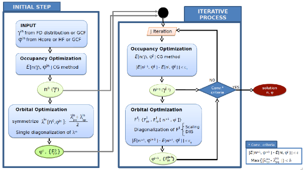
Figure 2: Flowchart in DoNOF

Fig. 2 depicts the flowchart in DoNOF. The procedure is divided into two fundamental steps. An initial one, which main objective is to generate the diagonal elements of the symmetric matrix $\mathcal{F}$, and the iterative step where it is optimized by occupancies and orbitals separately.

In the initial step, the guess for molecular orbitals $\left\{\varphi_{p}^{in}\right\}$ is generated directly from the core Hamiltonian or after a HF calculation. An energy optimization with respect to the auxiliary $\gamma$-variables is performed using the CG or L-BFGS methods. For this purpose, initial $\left\{\gamma_{p}^{in}\right\}$ corresponding to a Fermi-Dirac (FD) distribution of the ONs is generally used. For the ONs $\left\{n_{p}^{0}\right\}$ obtained according to Eqs. (19) and (21) from resulting $\left\{\gamma_{p}^{0}\right\}$, a single diagonalization of the symmetrized $\lambda$-matrix with $\left\{\varphi_{p}^{in}\right\}$, $\left(\lambda_{pq}^{in}+\lambda_{qp}^{in}\right)/2$, is carried out that affords $\left\{\varphi_{p}^{0}\right\}$ and a suitable start guess $\left\{\mathcal{F}_{pp}^{0}\right\}$.

In the iterative step, $\gamma^{j+1}$ is obtained for fixed NOs $\varphi^{j}$ by the unconstrained optimization of $E\left[n\left(\gamma\right),\varphi^{j}\right]$. Then, the symmetric matrix $\mathcal{F}^{j}$ is formed with the resulting diagonal elements of the previous step, and the off-diagonal elements given by Eq. (32) using $n^{j+1}\left(\gamma^{j+1}\right)$ and $\varphi^{j}$. After diagonalization of $\mathcal{F}^{j}$, new NOs $\varphi^{j+1}$ and diagonal elements $\left\{\mathcal{F}_{pp}^{j+1}\right\}$ are obtained.

Three criteria of energy convergence are used, one for occupancy optimization, another for orbital optimization and finally a global one. Each criterion consists of monitoring the electronic energy of each iteration and requires that two successive values differ by no more than a threshold, namely,

$$\left|E\left[n^{j+1},\varphi^{j}\right]-E\left[n^{j},\varphi^{j}\right]\right|<\varepsilon_{n}$$ (44)

$$\left|E\left[n^{j+1},\varphi^{j+1}\right]-E\left[n^{j+1},\varphi^{j}\right]\right|<\varepsilon_{\varphi}$$ (45)

$$\left|E\left[n^{j+1},\varphi^{j+1}\right]-E\left[n^{j},\varphi^{j}\right]\right|<\varepsilon$$ (46)

It is worth noting that we do not determine whether the new NOs $\varphi^{j+1}$ (ONs $n^{j+1}$) are the same as previous $\varphi^{j}$ ($n^{j}$). A robust criterion that prevails over the three energy criteria is to assess the symmetry of the matrix of the Lagrange multipliers, namely, the maximum of the off-diagonal differences to be less than $\delta$:

$$Max\left\{\left|\lambda_{qp}^{j+1}-\lambda_{pq}^{j+1}\right|\right\}<\delta$$ (47)

To help convergence, the scaling of $\mathcal{F}$ is used as well as the DIIS technique explained above. If the convergence criteria are reached, then the solution represented by optimal $\left\{n_{p},\varphi_{p}\right\}$ can be employed to calculate other quantities of interest.

IV Molecular Properties

At the present stage, the program computes molecular properties such as vertical ionization potentials by means of the extended Koopmans’ theorem (Piris et al., 2012), Mulliken population analysis (Mulliken, 1955), and electric dipole, quadrupole and octupole moments (Mitxelena and Piris, 2016). We provide the RDMs in the atomic and molecular bases if necessary, and a wavefunction (WFN) file for performing further quantitative and visual analyses of molecular systems.

The 1RDM and Lagrangian cannot be simultaneously brought to the diagonal form in approximate NOFs. DoNOF works on the NO representation, where the 1RDM is diagonal, but $\lambda$ is only a symmetric matrix. The program can provide a complementary canonical representation (Piris et al., 2013a) of the one-electron picture in molecules where $\lambda$ is diagonal, but not the 1RDM. This equivalent representation affords delocalized molecular orbitals adapted to the symmetry of the molecule. Combining both representations we have the whole picture concerning the ONs and orbital energies in NOF theory. Currently both types of orbitals can be displayed using the DoNOF output file which can be read by the GMOLDEN programm (Schaftenaar, ) duly modified by us.

In the case of PNOF5, an APSG with the expansion coefficients explicitly expressed by the ONs can generate (Piris et al., 2013b) the functional too. Our code offers the option of knowing the expansion coefficients of the APSG generating wavefunction. In addition, the treatment of an extended system at a fractional cost of the entire calculation can also be achieved using a thermodynamic fragment energy method in the context of NOF theory (Lopez and Piris, 2015).

Geometry optimization is, together with single-point energy calculations, the most used procedure in electronic structure calculations. DoNOF computes the analytic energy gradients (Mitxelena and Piris, 2017) with respect to nuclear motion without resorting to linear response theory. It is worth noting that our implementation of the geometry optimization can also be applied to non-singlet systems as long as the spin-multiplet formalism mentioned above is used (Mitxelena and Piris, 2020c). This efficient computation of analytical gradients, analogous to gradient calculations at the HF level of theory, allows to locate and characterize the critical points on the energy surface.

In contrast to first-order energy derivatives, the calculation of the second-order analytic derivatives requires the knowledge of NOs and ONs at the perturbed geometry (Mitxelena and Piris, 2018). Thus, since a set of coupled-perturbed equations must be solved to analytically obtain the Hessian in NOF theory, the corresponding computational cost increases dramatically. Consequently, in the current implementation, the Hessian is obtained by numerical differentiation of analytical gradients (Mitxelena et al., 2019).

V Dynamic Correlation

Current NOFs based on electron pairing take into account most of the non-dynamical effects, and also an important part of the dynamical electron correlation corresponding to the intrapair interactions. Consequently, electron-pairing-based NOFs produce (Piris, 2017b; Piris et al., 2013b) results that are in good agreement with accurate wavefunction-based methods for small systems, where electron correlation effects are almost entirely intrapair. When the number of pairs increases, NOF values deteriorate especially in those regions where dynamic correlation prevails. It is therefore mandatory to add the inter-space dynamic electron correlation to improve calculations.

The second-order Møller–Plesset (MP2) perturbation theory is the simplest way of properly incorporating dynamic correlation effects. In DoNOF, the recently proposed (Piris, 2019, 2017b, 2018b) NOF-MP2 method can be used to obtain a good balance of both static (non-dynamic) and dynamic electron correlation. The zeroth-order Hamiltonian is constructed from a closed-shell-like Fock operator that contains a HF density matrix with doubly ($2n_{g}=2$) and singly ($2n_{g}=1$) occupied orbitals. The electronic energy is then calculated by the expression

$$E=\tilde{E}_{hf}+E^{corr}=\tilde{E}_{hf}+E^{sta}+E^{dyn}$$ (48)

where $\tilde{E}_{hf}$ is the HF-like energy obtained with the NOs,

$$\tilde{E}_{hf}=2\sum\limits_{g=1}^{\mathrm{N}_{\Omega}}\mathcal{H}_{gg}+\sum_{f,g=1}^{\mathrm{N}_{\Omega}}\left(2\mathcal{J}_{fg}-\mathcal{K}_{fg}\right)-\sum_{g=\frac{\mathrm{N_{II}}}{2}+1}^{\mathrm{N}_{\Omega}}\frac{\mathcal{J}_{gg}}{4}$$ (49)

$E^{sta}$ is the sum of the static intra-space and inter-space correlation energies,

$$\begin{array}[]{c}E^{sta}=\sum\limits_{g=1}^{\mathrm{N_{II}/2}}\sum\limits_{q\neq p}\sqrt{\Lambda_{q}\Lambda_{p}}\,\Pi_{qp}\mathcal{\,K}_{pq}\\ \\ -4\sum\limits_{f\neq g}^{\mathrm{\mathrm{N}_{\Omega}}}\sum\limits_{p\in\Omega_{f}}\sum\limits_{q\in\Omega_{g}}\Phi_{q}^{2}\Phi_{p}^{2}\mathcal{K}_{pq}\end{array}$$ (50)

and $E^{dyn}$ is obtained from a modified second-order MP2 correction,

$$E^{dyn}=\sum\limits_{g,f=1}^{\mathrm{\mathrm{N}_{\Omega}}}\;\sum\limits_{p,q>\mathrm{N}_{\Omega}}^{\mathrm{N}_{B}}A_{g}A_{f}\left\langle gf\right|\left.pq\right\rangle\left[2T_{pq}^{gf}\right.\left.-T_{pq}^{fg}\right]$$ (51)

where

$$A_{g}=\left\{\begin{array}[]{c}1\,,\quad 1\leq g\leq\frac{\mathrm{N_{II}}}{2}\\ \frac{\mathrm{1}}{2},\>\frac{\mathrm{N_{II}}}{2}<g\leq\mathrm{N}_{\Omega}\end{array}\right.$$ (52)

$\mathrm{N}_{B}$ is the number of basis functions, and $T_{pq}^{fg}$ are the amplitudes of the doubly excited configurations obtained by solving modified equations for the MP2 residuals (Piris, 2018b). An important feature of the method is that double counting is avoided by taking the amount of static and dynamic correlation in each orbital as a function of its occupancy. In Eq. (50), for instance, $\Lambda_{p}=1-\left|1-2n_{p}\right|$ goes from zero for empty or fully occupied orbitals to one if the orbital is half occupied.

It is convenient to take into account the inter-pair static correction in the reference-used NOF from the outset, thus preventing the ONs and NOs from suffering an inter-pair non-dynamic influence, however small, in the dynamic correlation domains. This led us to correlate the motion of electrons with parallel and opposite spins belonging to different subspaces ($\Omega_{f}\neq\Omega{}_{g}$) as

$$E_{fg}=\sum\limits_{p\in\Omega_{f}}\sum\limits_{q\in\Omega_{g}}\left[n_{q}n_{p}\left(2\mathcal{J}_{pq}-\mathcal{K}_{pq}\right)-4\Phi_{q}^{2}\Phi_{p}^{2}\mathcal{K}_{pq}\right]$$ (53)

The functional (15), (16), and (53) instead of Eq. (17) was called static PNOF7 (PNOF7s) for multiplets (Piris, 2018b). Note that the difference between the PNOF7 and PNOF7s functionals lies in the last term of $E_{fg}$ that correlates electrons with opposite spins. In the case of PNOF7s, the quadratic dependence of the product $4\Phi_{q}^{2}\Phi_{p}^{2}$ practically eliminates this term when the ONs are close to zero or one, that is, when dynamic correlation is present. On the other hand, its value is maximum when the orbitals are half occupied, that is, static correlation dominates, coinciding with the PNOF7 values of the $E_{fg}$ in Eq. (17).

VI Illustrative example: water molecule

The water molecule is probably the most studied system in quantum chemistry. We have accurate experimental data at our disposal for $H_{2}O$, therefore it is an ideal candidate to test our code and display the capabilities of DoNOF. In this section, we employ the correlation-consistent basis set series cc-pVXZ (X = D, T, Q) developed by Dunning and coworkers (Dunning and Dunning Jr., 1989) obtained from use of the basis set exchange software (Pritchard et al., 2019). For comparison, we report the experimental data as well as other accurate theoretical calculations taken from the NIST CCCBDB database (Johnson III, 2019).

Convergence was accomplished in all cases for the three energy criteria $\varepsilon_{n},\,\varepsilon_{\varphi}=10^{-10},\,\varepsilon=10^{-8}$, and a tolerance $\delta=10^{-4}$, in accordance to the symmetry criterion of the matrix of the Lagrange multipliers. A curious fact is that, in the case of a lower energy criterion $\varepsilon$, the accuracy achieved in most cases exceeds the required value when the $\delta$-tolerance is reached, confirming that it is the strongest of all the criteria discussed in the subsection III.4.

Table 1: Occupation numbers of the water molecule at the experimental equlibrium geometry ($R_{OH}=0.9578\textrm{\r{A}}$, $\varangle HOH=104.5\text{\textordmasculine}$) and atomic dissociation. The cc-pVDZ basis set was employed. $\mathrm{N}_{g}=4$.

MO	Experimental Geometry			Atomic Dissociation
	PNOF5	PNOF7s	PNOF7	PNOF5	PNOF7s	PNOF7
1	2.000	2.000	2.000	2.000	2.000	2.000
2	1.980	1.980	1.971	1.000	1.000	1.000
3	1.980	1.980	1.971	1.000	1.000	1.000
4	1.992	1.992	1.988	1.993	1.991	1.976
5	1.992	1.992	1.988	1.993	1.991	1.976
6	0.000	0.000	0.000	0.000	0.001	0.002
7	0.001	0.001	0.001	0.001	0.001	0.003
8	0.007	0.007	0.011	0.005	0.007	0.016
9	0.000	0.000	0.002	0.001	0.001	0.003
10	0.000	0.000	0.000	0.000	0.001	0.002
11	0.000	0.000	0.002	0.001	0.001	0.003
12	0.001	0.001	0.001	0.001	0.001	0.003
13	0.007	0.007	0.011	0.005	0.007	0.016
14	0.001	0.001	0.001	0.000	0.000	0.000
15	0.002	0.002	0.003	0.000	0.000	0.001
16	0.017	0.017	0.025	1.000	1.000	0.998
17	0.001	0.001	0.001	0.000	0.000	0.001
18	0.001	0.001	0.001	0.000	0.000	0.001
19	0.017	0.017	0.025	1.000	1.000	0.998
20	0.002	0.002	0.003	0.000	0.000	0.001
21	0.000	0.000	0.000	0.000	0.000	0.000
22	0.000	0.000	0.000	0.000	0.000	0.000
23	0.000	0.000	0.000	0.000	0.000	0.000
24	0.000	0.000	0.000	0.000	0.000	0.000
25	0.000	0.000	0.000	0.000	0.000	0.000

We begin by selecting the minimum value of $\mathrm{N}_{g}$ required to correctly describe the electron pairs that make up the system, which in the case of water are five pairs. Our electron-pair-based functionals are not capable of recovering the entire dynamic correlation, so we must resort to perturbative corrections if we want to obtain significant total energies. Consequently, it is convenient to reduce the value of $\mathrm{N}_{g}$ considering only the ONs that do not exceed a certain threshold, e.g. 0.01. Small ONs are known to contribute solely to dynamic correlation and slow down convergence by making the surface where minimization is performed flatter.

We must recall that we assumed an equal number $\mathrm{N}_{g}$ for all subspaces that is determined by the basis set used. In general, the best strategy is to consider the smallest basis set to determine which are the orbitals that determine the static correlation in different significant geometries, and thus define the minimum required value of $\mathrm{N}_{g}$.

Table 1 shows the ONs obtained with PNOF5, PNOF7s and PNOF7 at the experimental equilibrium geometry. In principle, a geometry close to equilibrium, e.g., the geometry optimized at the HF theory level, is adequate. The table also includes the ONs in the atomic dissociation. For the latter, the distance between the oxygen atom and each hydrogen atom was taken equal to 1000 Å. The $\mathrm{N}_{g}$ value corresponding to the cc-pVDZ basis set was found to be four.

Inspection of the data collected in this table reveals that for $H_{2}O$ the typical bonding-anti-bonding orbital scheme is adequate. Indeed, the ONs of the weakly occupied NOs 8, 13, 16 and 19, determine that the value of $\mathrm{N}_{g}=1$ is sufficient. Furthermore, taking into account how full the first orbital is, we can also freeze its occupancy at 2. Note that the NOs together with their occupancies adapt to the problem during the optimization process. We have not rearranged the ONs since our objective is to highlight the coupling scheme adopted to form the subspaces (see Fig. 1).

In Table 2, we can find the ONs obtained by establishing $\mathrm{N}_{g}=1$. The results confirm that no significant differences are obtained, although they are better adapted to the symmetry of the system when the number of optimized $\gamma$-variables is reduced. Hereinafter, all our results refer to this bonding-anti-bonding orbital scheme.

Table 2: Occupation numbers of the water molecule at the experimental equlibrium geometry ($R_{OH}=0.9578\textrm{\r{A}}$, $\varangle HOH=104.5\text{\textordmasculine}$) and atomic dissociation. The cc-pVDZ basis set was employed. $\mathrm{N}_{g}=1$.

MO	Experimental Geometry			Atomic Dissociation
	PNOF5	PNOF7s	PNOF7	PNOF5	PNOF7s	PNOF7
1	2.00000	2.00000	2.00000	2.00000	2.00000	2.00000
2	1.98183	1.98158	1.97575	1.00000	1.00000	1.00000
3	1.98183	1.98158	1.97575	1.00000	1.00000	1.00000
4	1.99306	1.99297	1.99051	1.99464	1.99242	1.98303
5	1.99306	1.99297	1.99051	1.99464	1.99242	1.98303
6	0.00694	0.00703	0.00949	0.00536	0.00758	0.01697
7	0.00694	0.00703	0.00949	0.00536	0.00758	0.01697
8	0.01817	0.01842	0.02425	1.00000	1.00000	1.00000
9	0.01817	0.01842	0.02425	1.00000	1.00000	1.00000

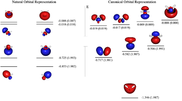
Figure 3: Valence molecular orbitals calculated using PNOF7s/cc-pVDZ level of theory at the equilibrium geometry. Corresponding diagonal Lagrange multipliers in Hartrees, and 1RDM diagonal elements in parentheses, are also reported

The PNOF7s valence NOs are shown in Fig. 3 at the experimental equilibrium geometry. Recall that in the NO representation, the ONs are well defined but not the orbital energies. DoNOF provides the complementary canonical orbital (CO) representation included on the right side of the figure, where orbital energies correspond to the diagonal elements of the matrix of Langrange multipliers. Regrettably, we cannot assign ONs to the orbitals in the CO representation. In fact, the maximum 1RDM off-diagonal element is 0.028 at the PNOF7s/cc-pVDZ level of theory. When 1RDM off-diagional elements are small enough, the negative values of CO energies below the Fermi level provides a good approximation to the ionization potentials (Piris et al., 2013a).

In Fig. 3, we observe that NOs closely match the image emerging from the chemical bonding arguments: the O atom has $sp3$ hybridization, two of orbitals are used to bind to H atoms, leading to two degenerate OH $\sigma$ bonds, and the remaining two are degenerated lone pairs. On the other hand, in the CO representation, the orbitals obtained adapt to the molecular symmetry and resemble those obtained by the usual molecular orbital theories, for example, HF. Both representations provide the complete picture of occupancies and orbital energies.

The next step is to optimize the geometry of the water molecule for each level of theory. We use HF geometries as starting points to PNOF optimizations. Table 3 shows the errors in OH bond lengths and HOH bond angle with respect to the experimental structural data. According to the errors, PNOF5 and PNOF7s provide ground-state equilibrium bond-distances comparable to those of the MP2 and CCSD(T), whereas PNOF7 deviates slightly from these accurate wavefunction-based methods. Note that the results obtained with all three functionals for the HOH bond angle are excellent.

Table 3: Differences of the optimized geometry with respect to experimental data ($R_{OH}=0.9578\textrm{\r{A}}$, $\varangle HOH=104.5\text{\textordmasculine}$)

Method	cc-pVDZ		cc-pVTZ		cc-pVQZ
	$R_{OH}$(Å)	$\varangle\left(\text{\textdegree}\right)$	$R_{OH}$(Å)	$\varangle\left(\text{\textdegree}\right)$	$R_{OH}$(Å)	$\varangle\left(\text{\textdegree}\right)$
PNOF5	0.0072	-1.2	0.0005	0.3	-0.0007	0.6
PNOF7s	0.0075	-1.2	0.0007	0.3	-0.0004	0.6
PNOF7	0.0134	-1.7	0.0066	-0.2	0.0052	0.1
MP2	0.0071	-2.6	0.0012	-1.0	-0.0001	-0.5
CCSD(T)	0.0086	-2.5	0.0017	-0.9	0.0001	-0.4

A comparison between harmonic vibrational frequencies obtained by using PNOF5, PNOF7s, PNOF7, MP2, and CCSD(T), with respect to experimental fundamentals is displayed in Table 4. According to reported values, all functionals show good agreement with MP2 and CCSD(T). The largest error of 180 cm^-1 corresponds to the third vibrational mode computed with PNOF7 which, as mentioned above, can take an excess of static correlation in the equilibrium region that corresponds to the dynamic inter-pair correlation. The frequencies obtained with MP2 indicate that the NOF-MP2 method could lead to excellent results, a fact that we have verified in dimers (Piris, 2017b).

Table 4: Differences in harmonic vibrational frequencies (cm^-1) with respect to experimental data (3832, 1649, 3943)

Method	cc-pVDZ			cc-pVTZ			cc-pVQZ
PNOF5	-37	104	-65	-8	86	-34	11	79	-16
PNOF7s	-45	105	-66	-9	130	19	34	128	30
PNOF7	-162	82	-180	-125	56	-146	-128	5	-142
MP2	20	29	28	24	3	34	23	-6	35
CCSD(T)	-12	41	-17	8	19	2	13	10	9

Unfortunately, analytical gradients for the NOF-MP2 method are not available in DoNOF. It is a purpose for the near future, but unlike PNOF gradients, NOF-MP2 gradients require the linear response to nuclear motion. Nevertheless, we have scanned the energy with respect to the OH distance and the HOH angle to obtain the potential energy surface (PES). This procedure is computationally expensive, so we only show the PES at the NOF-MP2/cc-pVDZ level of theory (Fig. 4).

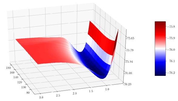
Figure 4: Symmetric dissociation of the water molecule at the NOF-MP2/cc-pVDZ level of theory. The minimum is at $R_{OH}=0.966\textrm{ \r{A}}$, $\varangle HOH=102.7\text{\textdegree}$

The minimum ($R_{OH}=0.966\,\textrm{\r{A}}$, $\varangle HOH=102.7\text{\textdegree}$) confirms that NOF-MP2 tends to lengthen bond distances and decrease bond angles with respect to PNOF7s. In the case of water, these trends would improve the PNOF7s marks with respect to the experimental values when the basis set increases.

It is worth noting that the NOFs used here as well as the NOF-MP2 method are size-consistent. This property implies that the energy of a water molecule obtained when the oxygen and hydrogens are infinitely separated is identical to the sum of the atomic energies. Furthermore, our NOFs are known to be the only ones that provide an integer number of electrons in the dissociated atoms when calculating Mulliken populations (Matxain et al., 2011). Both properties have been verified numerically in this study for $R_{OH}=1000\,\textrm{\r{A}}$.

In Table 5, we have collected the energies ($D_{e}$) required to disassemble a water molecule into its constituent atoms calculated at different levels of theory. Recall that MP2 and CCSD(T) fail at the dissociation limit of water, so these $D_{e}$ values have been calculated as the difference between the energy of the three atoms and the energy of water at equilibrium. In addition, MP2 and CCSD(T) employ unrestricted formulations to characterize spin-uncompensated systems.

Table 5: Theoretical binding energies ($D_{e}$) in kcal/mol at 0K

Method	cc-pVDZ	cc-pVTZ	cc-pVQZ
MP2	210.8	228.5	234.0
CCSD(T)	208.8	225.0	229.9
NOF-MP2	222.2	242.2	247.4

The values of $D_{e}$ obtained with our NOFs are not reported in Table 5 since they underestimate $D_{e}$ by approximately 50 kcal/mol due to the aforementioned lack of an important part of the dynamic correlation in the equilibrium region. Conversely, NOF-MP2 adequately recovers the dynamic correlation and yields more reasonable values of the binding energy. We can see that these values, however, are higher than those obtained with the MP2 and CCSD(T) methods.

In the case of singlets at the equilibrium geometry, NOF-MP2 provides total energies similar to those of the MP2 method (Piris, 2018b), whereas CCSD(T) can further reduce energy with the triple contributions. Accordingly, the differences in $D_{e}$ may be associated with uneven descriptions of the dissociated oxygen atom in its triplet state. Indeed, the oxygen total spin is conserved with NOF-MP2 in contrast to the MP2 and CCSD(T) methods. This symmetry violation leads to lower energy values for the triplet state. Table 6 shows the differences of the singlet-triplet gap with respect to the experiment for the oxygen atom calculated with the three methods. From the Table, we can conclude that the best description of the singlet-triplet gap is given by the NOF-MP2 method, whereas MP2 significantly overestimates the energy of the triplet state. The CCSD(T) method compensates for the spin violation in the triplet state with the best description of the electron correlation in the singlet state.

Table 6: Energy differences (kcal/mol) in the singlet-triplet gap of the oxygen atom with respect to the experiment (45.4 kcal/mol)

Method	cc-pVDZ	cc-pVTZ	cc-pVQZ
MP2	23.4	21.1	19.8
CCSD(T)	6.9	5.7	5.0
NOF-MP2	2.8	0.1	-0.8

Next, let us discuss two more properties that we can obtain with our code in the corresponding optimized geometries, namely, ionization potentials and electrostatic moments.

Table 7 lists the differences of the lowest vertical ionization potential (LVIP) with respect to the experimental values obtained by PNOF5, PNOF7s, PNOF7 using the extended Koopmans’ theorem (EKT) (Piris et al., 2012). For comparison, the Koopmans’ theorem (KT) LVIP has also been included. It has long been recognized that, in general, there is an excellent agreement between the KT LVIPs and the experimental data because of the fortuitous cancellation of the electron correlation and orbital relaxation effects. However, in the case of water, the KT greatly overestimates the LVIP.

Table 7: Differences in eV of the lowest vertical ionization potentials with respect to the experimental data (12.600 eV). PNOF values were obtained by means of the extended Koopmans’ theorem (EKT)

Method	cc-pVDZ	cc-pVTZ	cc-pVQZ
Koopmans’	0.848	1.173	1.265
PNOF5	0.461	0.801	0.896
PNOF7s	0.458	0.798	0.892
PNOF7	0.394	0.726	0.815
$\Delta$NOFMP2*	-0.225	0.399	0.584

* The PNOF7s optimized geometry was used

A survey of Table 7 reveals that PNOF-EKT values improve those obtained by KT, a predominant trend previously observed in many systems (Piris et al., 2012). The EKT considers the electron correlation accounted by the specific functional, but neglects the orbital relaxation in the (N-1)-state. In order to include the dynamic correlation and take into account the orbital relaxation, we have calculated the LVIP as the energy difference between the positive ion in its doublet state and the neutral water molecule, at the NOF-MP2 level of theory using PNOF7s optimized geometries. These values appear in the table under the $\Delta$NOFMP2 notation. We can perceive an improvement in the $\Delta$NOFMP2 values approaching the experimental LVIP. However, neither method produces better agreement with the experiment when the size of the basis set improves.

Due to its increased electronegativity, the oxygen atom in the water molecule attracts the electrons shared with the hydrogen atoms in the covalent bonds. As a result, the O atom acquires a partial negative charge, while the H atoms have a partial positive charge. Additionally, the electron lone-pair on the oxygen forces the molecule to assume a bent structure. The latter avoids the cancellation of polar OH bonds, causing the entire water molecule to become polarized.

Tables 8 and 9 show the differences with respect to the experiment in the calculated electric dipole and quadrupole moments at the HF, PNOF5, PNOF7s, PNOF7 and CCSD levels of theory, respectively. The latter were computed with respect to the center of mass using the corresponding optimized geometry for each theoretical method. Since the traceless definition of the quadrupole moment is employed, two components are sufficient to determined it. The octupole moment has been excluded from this study, since the latter is only significant when the lower order electric moments are zero, e.g. in tetrahedral molecules (Mitxelena and Piris, 2016).

Table 8: Differences in Debye of the water dipole moment calculated at the optimized geometry with respect to the experimental data (1.855 Debye)

Method	cc-pVDZ	cc-pVTZ	cc-pVQZ
HF	0.189	0.133	0.110
PNOF5	0.174	0.128	0.102
PNOF7s	0.173	0.128	0.101
PNOF7	0.161	0.117	0.091
CCSD	0.128	0.072	0.055

Inspection of the data collected in these tables reveals that PNOFs produce molecular electric moments comparable to those of CCSD. Interestingly, in the case of the water molecule, the HF results are in line with those obtained by methods that include electron correlation, although this is generally not the case (Mitxelena and Piris, 2016). According to Tables 8 and 9, the charge distribution of molecules is adequately described using any of the PNOF approaches. However, in view of the aforementioned missing interpair dynamical correlation, it is important to study the electrical properties using the NOF-MP2 method. A work in this direction is underway.

Table 9: Differences in Buckingham of the water quadrupole moment components calculated at the optimized geometry with respect to the experimental data ($Q_{xx}=-2.500,Q_{yy}=2.630$)

Method	cc-pVDZ		cc-pVTZ		cc-pVQZ
	$Q_{xx}$	$Q_{yy}$	$Q_{xx}$	$Q_{yy}$	$Q_{xx}$	$Q_{yy}$
HF	0.504	-0.324	0.351	-0.087	0.295	-0.011
PNOF5	0.559	-0.363	0.358	-0.103	0.291	-0.016
PNOF7s	0.559	-0.364	0.358	-0.104	0.291	-0.017
PNOF7	0.493	-0.311	0.365	-0.118	0.294	-0.025
CCSD	0.560	-0.502	0.368	-0.205	0.285	-0.086

VII Summary

In this work, we have presented the DoNOF program for computational chemistry calculations based on the natural orbital functional (NOF) theory, where the electronic structure is described in terms of the natural orbitals (NOs) and their occupation numbers (ONs).

In section I, we discussed how NOF approximations can be useful to quantum chemistry as an alternative formalism to both density functional and wavefunction methods. Special emphasis was placed on the need for functional N-representability and the conservation of the total spin of the system under study.

In section II, we reviewed the fundamental aspects of the electron-pairing-based NOF theory for multiplets. The reconstructions developed in our group for the two-particle reduced density matrix in terms of the ONs were briefly presented. They led to the appearance of different versions of PNOF that can provide a correct description of systems with a multiconfigurational nature, one of the biggest challenges for DFs.

Our self-consistent algorithm for optimizing an energy functional with respect to the NOs and their ONs was introduced in section III. We described how the constrained nonlinear programming problem for ONs can be treated as unconstrained optimization, with corresponding computational savings. The specific techniques that help obtain convergence in the orbital optimization were discussed, namely the direct inversion of the iterative subspace (DIIS) extrapolation technique, and the variable scaling of the symmetric matrix subject to iterative diagonalizations. It is important to note that, although these techniques have confirmed their practical value, the number of iterations is still very high, so more convergence techniques must be implemented in the code. Depending on the desired precision, computational times can be long, limiting the calculations to small molecules with extended basis sets or modestly sized molecules with modest basis sets. An overview of the computational procedure in DoNOF is given at the end of this section.

Section IV was dedicated to molecular properties that can be calculated with DoNOF once the NOF solution is reached. The orbital-invariant formulation of the NOF-MP2 method was briefly presented in section V. The latter allows us to remedy the lack of the interpair dynamic correlation inherent in $\mathcal{JKL}$-functionals developed by us. The single-reference NOF-MP2 method improves the absolute energies over the PNOF values by bringing them closer to the values obtained by accurate wavefunction-based methods.

The capabilities of DoNOF were discussed in section VI through the water molecule. This included analysis of molecular orbitals, ionization potential, electric moments, optimized geometry, harmonic vibrational frequencies, binding energy, and potential energy surface of the $H_{2}O$ symmetric dissociation. Consequently, DoNOF can calculate the energy and a variety of properties of any isolated molecule in its ground state, regardless of the total spin value of the system. It is especially important when one encounters near degeneracies, such as those that occur during bond-breaking processes, near transition states in chemical reactions or transition metal compounds. However, at present calculations of excited electronic states, the influence of a solvent, or relativistic effects cannot be performed. It is anticipated that these features will be implemented into DoNOF in the near future.

To extend the calculations with DoNOF to larger systems, in addition to making the iterative process more effective and efficient, new parallel implementations of other computationally demanding tasks are needed. On the other hand, the local spatial nature of NOs could be exploited to achieve a better scaling of the code with respect to the number of basis functions. It has been shown with other methods that an important source of computational savings is the neglect of correlation for pairs of very distant localized orbitals. Consequently, an improved scaling could be achieved by adopting a preselection procedure for the density matrices involved that will reduce the number of two-electron integrals.

We have shown the solution to longstanding problems in NOF theory, however new algorithms and capabilities are welcome to be included in the code. New parallel implementations of the DoNOF program tasks are also needed. We believe that DoNOF will benefit the community of quantum physicists and chemists, mainly those who start in the development of new functionals, and these in turn will improve the code by bringing new functionalities.

Acknowledgments: The authors greatly appreciate Dr. Eduard Matito’s parallel implementation of the four-index transformation of the electron repulsion integrals that substantially improved the performance of DoNOF. The authors also appreciate for technical and human support provided by IZO-SGI SGIker of UPV/EHU and European funding (ERDF and ESF). Financial support comes from MCIU/AEI/FEDER, UE (PGC2018-097529-B-100) and Eusko Jaurlaritza (Ref. IT1254-19).

References

- Husimi (1940) K. Husimi, Proc. Phys. Math. Soc. Jpn. 22, 264 (1940).
- Mazziotti (2012a) D. A. Mazziotti, Chem. Rev. 112, 244 (2012a).
- Gilbert (1975) T. L. Gilbert, Phys. Rev. B 12, 2111 (1975).
- Valone (1980) S. M. Valone, J. Chem. Phys. 73, 1344 (1980).
- Hohenberg and Kohn (1964) P. Hohenberg and W. Kohn, Phys. Rev. 136, B864 (1964).
- Valone (1991) S. M. Valone, Phys. Rev. B 44, 1509 (1991).
- Mori-Sánchez and Cohen (2018) P. Mori-Sánchez and A. J. Cohen, J. Phys. Chem. Lett. 9, 4910 (2018).
- Levy (1979) M. Levy, Proc. Natl. Acad. Sci. USA 76, 6062 (1979).
- Lieb (1983) E. H. Lieb, Int. J. Quantum Chem. 24, 243 (1983).
- Burke (2012) K. Burke, J. Chem. Phys. 136, 150901 (2012).
- Becke (2014) A. D. Becke, J. Chem. Phys. 140, 18A301 (2014).
- Pernal and Giesbertz (2016) K. Pernal and K. J. H. Giesbertz, Top. Curr. Chem. 368, 125 (2016).
- Cohen et al. (2012) A. J. Cohen, P. Mori-Sánchez, and W. Yang, Chem. Rev. 112, 289 (2012).
- Coleman (1963) A. J. Coleman, Rev. Mod. Phys. 35, 668 (1963).
- Piris (2017a) M. Piris, in Many-body approaches Differ. scales a Tribut. to N. H. March Ocas. his 90th Birthd., edited by G. G. N. Angilella and C. Amovilli (Springer, New York, NY, USA, 2017a), chap. 22, pp. 231–247.
- Ayers and Liu (2007) P. W. Ayers and S. Liu, Phys. Rev. A 75, 022514 (2007).
- Ludeña et al. (2013) E. V. Ludeña, F. J. Torres, and C. Costa, J. Mod. Phys. 04, 391 (2013).
- Rodríguez-Mayorga et al. (2017) M. Rodríguez-Mayorga, E. Ramos-Cordoba, M. Via-Nadal, M. Piris, and E. Matito, Phys. Chem. Chem. Phys 19, 24029 (2017).
- Piris (2006) M. Piris, Int. J. Quantum Chem. 106, 1093 (2006).
- Piris et al. (2010) M. Piris, J. M. Matxain, X. Lopez, and J. M. Ugalde, J. Chem. Phys. 133, 111101 (2010).
- Piris et al. (2009) M. Piris, J. M. Matxain, X. Lopez, and J. M. Ugalde, J. Chem. Phys. 131, 21102 (2009).
- Quintero-Monsebaiz et al. (2019) R. Quintero-Monsebaiz, I. Mitxelena, M. Rodríguez-Mayorga, A. Vela, and M. Piris, J. Phys. Condens. Matter 31, 165501 (2019).
- Piris (2019) M. Piris, Phys. Rev. A 100, 32508 (2019).
- Piris (2007) M. Piris, in Reduced-Density-Matrix Mech. with Appl. to many-electron atoms Mol., edited by D. A. Mazziotti (John Wiley and Sons, Hoboken, New Jersey, USA, 2007), chap. 14, pp. 387–427.
- Piris (2013) M. Piris, Int. J. Quantum Chem. 113, 620 (2013).
- Piris and Ugalde (2014) M. Piris and J. M. Ugalde, Int. J. Quantum Chem. 114, 1169 (2014).
- Lopez et al. (2010) X. Lopez, M. Piris, J. M. Matxain, and J. M. Ugalde, Phys. Chem. Chem. Phys. 12, 12931 (2010).
- Ruipérez et al. (2013) F. Ruipérez, M. Piris, J. M. Ugalde, and J. M. Matxain, Phys. Chem. Chem. Phys. 15, 2055 (2013).
- Piris (2018a) M. Piris, in Theor. Quantum Chem. Daw. 21st Century, edited by T. Chakraborty and R. Carbó-Dorca (Apple Academic Press, 2018a), chap. 22, pp. 593–620.
- Matxain et al. (2011) J. M. Matxain, M. Piris, F. Ruipérez, X. Lopez, and J. M. Ugalde, Phys. Chem. Chem. Phys. 13, 20129 (2011).
- Piris et al. (2016) M. Piris, X. Lopez, and s. M. Ugalde, Chem. - A Eur. J. 22, 4109 (2016).
- Mitxelena and Piris (2020a) I. Mitxelena and M. Piris, J. Phys. Condens. Matter 32, 17LT01 (2020a).
- Mitxelena and Piris (2020b) I. Mitxelena and M. Piris, J. Chem. Phys. 152, 064108 (2020b).
- Piris (2017b) M. Piris, Phys. Rev. Lett. 119, 063002 (2017b).
- Mitxelena et al. (2018) I. Mitxelena, M. Rodríguez-Mayorga, and M. Piris, Eur. Phys. J. B 91, 109 (2018).
- Cohen and Baerends (2002) A. J. Cohen and E. J. Baerends, Chem. Phys. Lett. 364, 409 (2002).
- Herbert and Harriman (2003) J. M. Herbert and J. E. Harriman, J. Chem. Phys. 118, 10835 (2003).
- Piris and Ugalde (2009) M. Piris and J. M. Ugalde, J. Comput. Chem. 30, 2078 (2009).
- (39) In 2013, Dr. Eduard Matito carried out the parallel implementation in DoNOF of the four-index transformation so that the electron repulsion integrals move from the atomic to molecular representation.
- Pulay (1980) P. Pulay, Chem. Phys. Lett. 73, 393 (1980).
- Pulay (1982) P. Pulay, J. Comp. Chem. 3, 556 (1982).
- Piris et al. (2012) M. Piris, J. M. Matxain, X. Lopez, and J. M. Ugalde, J. Chem. Phys. 136, 174116 (2012).
- Mulliken (1955) R. S. Mulliken, J. Chem. Phys. 23, 1833 (1955).
- Mitxelena and Piris (2016) I. Mitxelena and M. Piris, J. Chem. Phys. 144, 204108 (2016).
- Piris et al. (2013a) M. Piris, J. M. Matxain, X. Lopez, and J. M. Ugalde, Theor. Chem. Acc. 132, 1298 (2013a).
- Mitxelena and Piris (2017) I. Mitxelena and M. Piris, J. Chem. Phys. 146, 014102 (2017).
- Mitxelena et al. (2019) I. Mitxelena, M. Piris, and J. M. Ugalde, in State Art Mol. Electron. Struct. Comput. Correl. Methods, Basis Sets More, edited by P. Hoggan and U. Ancarani (Academic Press, 2019), Advances in Quantum Chemistry, chap. 7, pp. 155–177.
- Piris (2018b) M. Piris, Phys. Rev. A 98, 022504 (2018b).
- Lopez and Piris (2019) X. Lopez and M. Piris, Theor. Chem. Acc. 138, 89 (2019).
- Mazziotti (2012b) D. A. Mazziotti, Phys. Rev. Lett. 108, 263002 (2012b).
- Piris (1999) M. Piris, J. Math. Chem. 25, 47 (1999).
- Lowdin and Shull (1955) P. O. Lowdin and H. Shull, Phys. Rev. 101, 1730 (1955).
- Piris et al. (2011) M. Piris, X. Lopez, F. Ruipérez, J. M. Matxain, and J. M. Ugalde, J. Chem. Phys. 134, 164102 (2011).
- Piris et al. (2013b) M. Piris, J. M. Matxain, and X. Lopez, J. Chem. Phys. 139, 234109 (2013b).
- Fletcher (2000) R. Fletcher, Practical Methods of Optimization (Wiley-Interscience, New York, NY, USA, 2000), 2nd ed., ISBN 978-0-471-49463-8.
- Saunders and Hillier (1973) V. R. Saunders and I. H. Hillier, Int. J. Quantum Chem. 7, 699 (1973).
- Schmidt et al. (1993) M. W. Schmidt, K. K. Baldridge, J. A. Boatz, S. T. Elbert, M. S. Gordon, J. H. Jensen, S. Koseki, N. Matsunaga, K. A. Nguyen, S. Su, et al., J. Comp. Chem. 14, 1347 (1993).
- Gordon and Schmidt (2005) M. S. Gordon and M. W. Schmidt, Theory and Applications of Computational Chemistry (Elsevier, 2005), ISBN 9780444517197.
- Pritchard et al. (2019) B. P. Pritchard, D. Altarawy, B. Didier, T. D. Gibson, and T. L. Windus, J. Chem. Inf. Model 59, 4814 (2019).
- Dupuis et al. (1989) M. Dupuis, J. D. Watts, H. O. Villar, and G. J. Hurst, Comput. Phys. Commun. 52, 415 (1989).
- Giesbertz (2016) K. J. H. Giesbertz, Phys. Chem. Chem. Phys. (2016).
- (62) G. Schaftenaar, GMOLDEN, CMBI, University of Nijmegen, The Netherlands, 1991, http://cheminf.cmbi.ru.nl/molden/molden.html.
- Lopez and Piris (2015) X. Lopez and M. Piris, Theor. Chem. Acc. 134, 151 (2015).
- Mitxelena and Piris (2020c) I. Mitxelena and M. Piris, J. Chem. Phys. 153, 044101 (2020c).
- Mitxelena and Piris (2018) I. Mitxelena and M. Piris, J. Math. Chem. 56, 1445 (2018).
- Dunning and Dunning Jr. (1989) T. H. Dunning and T. H. Dunning Jr., J. Chem. Phys. 90, 1007 (1989).
- Johnson III (2019) R. D. Johnson III, ed., NIST Computational Chemistry Comparison and Benchmark Database, NIST Standard Reference Database Number 101, Release 20 (2019).