Non-Hermitian extension of the Nambu–Jona-Lasinio model in 3+1 and 1+1 dimensions

Abstract

This paper presents a non-Hermitian $\mathcal{PT}$-symmetric extension of the Nambu–Jona-Lasinio (NJL) model of quantum chromodynamics in 3+1 and 1+1 dimensions. In 3+1 dimensions, the SU(2)-symmetric NJL Hamiltonian $\mathcal{H}_{\textrm{NJL}}=\bar{\psi}(-i\gamma^{k}\partial_{k}+m_{0})\psi-G[(\bar{\psi}\psi)^{2}+(\bar{\psi}i\gamma_{5}\vec{\tau}\psi)^{2}]$ is extended by the non-Hermitian, $\mathcal{PT}$- and chiral-symmetric bilinear term $ig\bar{\psi}\gamma_{5}B_{\mu}\gamma^{\mu}\psi$; in 1+1 dimensions, where $\mathcal{H}_{\textrm{NJL}}$ is a form of the Gross-Neveu model, it is extended by the non-Hermitian $\mathcal{PT}$-symmetric but chiral symmetry breaking term $g\bar{\psi}\gamma_{5}\psi$. In each case, the gap equation is derived and the effects of the non-Hermitian terms on the generated mass are studied. We have several findings: in previous calculations for the free Dirac equation modified to include non-Hermitian bilinear terms, contrary to expectation, no real mass spectrum can be obtained in the chiral limit; in these cases a nonzero bare fermion mass is essential for the realization of $\mathcal{PT}$ symmetry in the unbroken regime. Here, in the NJL model, in which four-point interactions are present, we do find real values for the mass spectrum also in the limit of vanishing bare masses in both 3+1 and 1+1 dimensions, at least for certain specific values of the non-Hermitian couplings $g$. Thus, the four-point interaction overrides the effects leading to $\mathcal{PT}$ symmetry-breaking for these parameter values. Further, we find that in both cases, in 3+1 and in 1+1 dimensions, the inclusion of a non-Hermitian bilinear term can contribute to the generated mass. In both models, this contribution can be tuned to be small; we thus fix the fermion mass to its value when $m_{0}=0$ in the absence of the non-Hermitian term, and then determine the value of the coupling required so as to generate a bare fermion mass. Finally, we find that in both cases, a rich phase structure emerges from the gap equation as a function of the coupling strengths.

I Introduction

The study of $\mathcal{PT}$ symmetry in quantum mechanics has brought to light that the combined conditions of invariance under both parity reflection and time reversal, $\mathbf{x}\to-\mathbf{x}$ and $t\to-t$, can lead to a real energy spectrum BB , a fact which today has led to the discovery of many novel and interesting physical effects, see, for example references cited in CMB . The concepts that have been developed have also been extended to non-Hermitian bosonic field-theoretic systems, which appear to behave similarly bhkss . All such systems share the feature that time reversal is even. However, non-Hermitian fermionic systems that have odd time-reversal symmetry have much more subtle structures JSM ; AMS ; ASR ; AS1 ; AS2 ; BKB .

In Ref. BKB we have focused on identifying Lorentz-invariant two-body interactions that are $\mathcal{PT}$ symmetric, but not Hermitian in both 3+1 and 1+1 dimensions, and we have investigated the resulting spectra in the context of free Dirac-like equations. Interestingly, we found there that $\mathcal{PT}$ symmetry is always realized in the broken phase unless we introduce a finite value of the bare or current fermion mass $m_{0}$. That is to say, the energy spectrum is always complex, except when the mass parameter $m_{0}\neq 0$ exceeds specific model parameter values.

This leads us to the subject of this current paper: What role do higher-order type interactions in fermionic systems play? To this end, we study an interacting, relativistic fermionic theory, that is extended by including non-Hermitian terms into the Hamiltonian. The Nambu–Jona-Lasinio (NJL) model NJL , which has been developed into an effective field theory of quantum chromodynamics (QCD), lends itself to this. One can study how the mechanism of chiral symmetry breaking functions within a theory of interacting fermions, and include effects of temperature, density, and strong fields SPK . Its Hamiltonian density, which contains four-point interactions, reads

$$\mathcal{H}_{\textrm{NJL}}=\bar{\psi}(-i\gamma^{k}\partial_{k}+m_{0})\psi-G[(\bar{\psi}\psi)^{2}+(\bar{\psi}i\gamma_{5}\vec{\tau}\psi)^{2}],$$ (1)

where $\gamma$ denotes the Dirac matrices, $\vec{\tau}$ represents the isospin SU(2) matrices, and $G$ is a coupling strength. The two interaction terms, $(\bar{\psi}\psi)^{2}$ and $(\bar{\psi}i\gamma_{5}\vec{\tau}\psi)^{2}$, in the given combination are necessary in order to preserve the chiral symmetry of the interaction for the two-flavor version of the model. On the other hand, the current quark mass, $m_{0}$, breaks the chiral symmetry of the Hamiltonian explicitly.

Spontaneous breaking of chiral symmetry occurs via a mechanism that parallels pairing in the Bardeen-Cooper-Schrieffer (BCS) theory of superconductivity bcs . In the BCS theory, pairing takes place between like particles, that is, electrons with opposite spins leggett . In the NJL model, the pairing takes place between particles and their antiparticles, that is, between fermions and antifermions ASR .

The fermions in the 3+1-dimensional NJL model have odd time-reversal symmetry: $\mathcal{T}^{2}=-\mathbbm{1}$. In this work, we extend the NJL model to incorporate non-Hermitian $\mathcal{PT}$- symmetric bilinear fermionic terms that also preserve chiral symmetry, and we investigate how these terms influence the mass generation. We show that, contrary to the results obtained in BKB , the extended model does admit a real solution for the mass in the chiral limit, when $m_{0}=0$, and that the non-Hermitian $\mathcal{PT}$-symmetric bilinear fermionic term can be tuned to generate a finite effective current quark mass, eliminating the need for the parameter $m_{0}$.

We contrast our results from the 3+1-dimensional model with those obtained by extending the 1+1-dimensional Gross-Neveu model by a non-Hermitian $\mathcal{PT}$-symmetric bilinear fermionic interaction. However, in this case, chiral symmetry is broken explicitly by the non-Hermitian term, so that the generation of mass is not surprising. In addition, this theory behaves as a bosonic theory, since $\mathcal{T}^{2}=\mathbbm{1}$.

This paper is organized as follows. In Sec. II, we study the 3+1-dimensional theory, first recapping the symmetry arguments in the context of the equations of motion for the modified free theory, then solving the gap equation and discussing the results. The 1+1-dimensional theory is developed in the same fashion in Sec. III. We conclude and summarize our main findings in the final section, Sec. IV.

II Non-Hermitian extension of the 3+1-dimensional NJL model

We build up the extension of the non-Hermitian NJL model in two stages: First we discuss the symmetries associated with including the non-Hermitian chirally symmetric bilinear into the free Dirac equation, since this is relevant for calculating the associated Green function. Then we set up the new gap equation, solve it and present our results.

II.1 Symmetries of the free theory modified by an axial-vector bilinear fermionic non-Hermitian term

In BKB it was demonstrated explicitly that the bilinear terms $i\bar{\psi}\gamma_{5}B_{\mu}\gamma^{\mu}\psi$ and $i\bar{\psi}T_{\mu\nu}\sigma^{\mu\nu}\psi$ are both non-Hermitian and invariant under the combination of parity reflection and time reversal. In this section, we will consider only the former term, $\Gamma=ig\bar{\psi}\gamma_{5}B_{\mu}\gamma^{\mu}\psi$, since (as we shall show) it is also invariant under a chiral transformation. Notationally, we use the Dirac representation of the gamma matrices BD ,

$$\gamma^{0}=\left(\begin{array}[]{cc}\mathbbm{1}&0\\ 0&-\mathbbm{1}\end{array}\right),\quad\quad\gamma^{k}=\left(\begin{array}[]{cc}0&\sigma^{k}\\ -\sigma^{k}&0\end{array}\right),$$

where $\sigma^{k}$ are the Pauli matrices and $\gamma_{5}=i\gamma^{0}\gamma^{1}\gamma^{2}\gamma^{3}$.

Combining the free Dirac Hamiltonian $\mathcal{H}_{F}=\bar{\psi}(-i\gamma^{k}\partial_{k}+m_{0})\psi$ with the bilinear interaction $\Gamma$ results in the modified free Hamiltonian

$$\mathcal{H}_{0}=\mathcal{H}_{F}+\Gamma=\bar{\psi}(-i\gamma^{k}\partial_{k}+m_{0}+ig\gamma_{5}B_{\mu}\gamma^{\mu})\psi,$$ (2)

from which one infers the equation of motion

$$(i\not{\partial}-m_{0}-ig\gamma_{5}B_{\mu}\gamma^{\mu})\psi(t,\mathbf{x})=0.$$ (3)

The usual parity and time-reversal operations for the spinors are defined as BD ,

$$\mathcal{P}:\psi(t,\mathbf{x})\to\mathcal{P}\psi(t,\mathbf{x})\mathcal{P}^{-1}=\gamma^{0}\psi(t,-\mathbf{x}),$$ (4)

$$\mathcal{T}:\psi(t,\mathbf{x})\to\mathcal{T}\psi(t,\mathbf{x})\mathcal{T}^{-1}=Z\psi^{*}(-t,\mathbf{x}),$$ (5)

where $Z=i\gamma^{1}\gamma^{3}$. We note that (5) implies $\mathcal{T}^{2}=-\mathbbm{1}$, that is, the time-reversal operator in 3+1 dimensions is odd.

By setting $\mathbf{x}\to-\mathbf{x}$ in (3), we have

$$\big{(}i\gamma^{0}\partial_{0}-i\gamma^{k}\partial_{k}-m_{0}-ig\gamma_{5}B_{0}\gamma^{0}-ig\gamma_{5}B_{k}\gamma^{k}\big{)}\psi(t,-\mathbf{x})=0.$$ (6)

Multiplying (6) from the left by $\gamma^{0}$, we obtain

$$[i\not{\partial}-m_{0}+ig(\gamma_{5}B_{0}\gamma^{0}-\gamma_{5}B_{k}\gamma^{k})]\gamma^{0}\psi(t,-\mathbf{x})=0,$$ (7)

where we have used the fact that $\gamma^{0}$ anti-commutes with $\gamma^{k}$ and $\gamma_{5}$. Equation (7) implies that (3) is not form invariant under parity reflection. On the other hand, taking the complex conjugate of (7) and replacing $t\to-t$ gives

$$\begin{split}\big{[}&i\gamma^{0}\partial_{0}-i\gamma^{1}\partial_{1}+i\gamma^{2}\partial_{2}-i\gamma^{3}\partial_{3}-m_{0}-ig\gamma_{5}B_{0}\gamma^{0}\\ &+ig\gamma_{5}B_{1}\gamma^{1}-ig\gamma_{5}B_{2}\gamma^{2}+ig\gamma_{5}B_{3}\gamma^{3}\big{]}\gamma^{0}\psi^{*}(-t,\mathbf{-x})=0,\end{split}$$ (8)

where we have used $(\gamma^{2})^{*}=-\gamma^{2}$. Multiplying this expression with $i\gamma^{1}\gamma^{3}$ from the left does lead to a form-invariant Dirac equation,

$$(i\not{\partial}-m_{0}-ig\gamma_{5}B_{\mu}\gamma^{\mu})\gamma^{0}[i\gamma^{1}\gamma^{3}]\psi^{*}(-t,-\mathbf{x})=0$$ (9)

or

$$(i\not{\partial}-m_{0}-ig\gamma_{5}B_{\mu}\gamma^{\mu})\mathcal{PT}\psi(t,\mathbf{x})=0.$$ (10)

The form invariance of (3) under the combined space-reflection and time-reversal symmetries implies that the spectrum of the modified free Hamiltonian (2) can be real.

Furthermore, in the chiral limit of vanishing bare mass $m_{0}$ Eq. (3) becomes

$$(i\not{\partial}-ig\gamma_{5}B_{\mu}\gamma^{\mu})\psi(t,\mathbf{x})=0,$$ (11)

which respects continuous chiral symmetry: under the transformation, $\psi\to e^{i\alpha\gamma_{5}}\psi$, where $\alpha\in\mathbb{R}$, (11) becomes

$$(i\not{\partial}-ig\gamma_{5}B_{\mu}\gamma^{\mu})e^{i\alpha\gamma_{5}}\psi=0.$$ (12)

Multiplying from the left by $e^{i\alpha\gamma_{5}}$, we find

$$(\mathbbm{1}+i\alpha\gamma_{5}+...)(i\not{\partial}-ig\gamma_{5}B_{\mu}\gamma^{\mu})e^{i\alpha\gamma_{5}}\psi=0,$$ (13)

which reduces to

$$(i\not{\partial}-ig\gamma_{5}B_{\mu}\gamma^{\mu})e^{-i\alpha\gamma_{5}}e^{i\alpha\gamma_{5}}\psi=0,$$ (14)

so that we recover (11).

II.2 The gap equation for the non-Hermitian NJL model

We define our non-Hermitian NJL model to be

$$\mathcal{H}=\mathcal{H}_{0}-G[(\bar{\psi}\psi)^{2}+(\bar{\psi}i\gamma_{5}\vec{\tau}\psi)^{2}]=\bar{\psi}(-i\gamma^{k}\partial_{k}+m_{0}+ig\gamma_{5}B_{\mu}\gamma^{\mu})\psi-G[(\bar{\psi}\psi)^{2}+(\bar{\psi}i\gamma_{5}\vec{\tau}\psi)^{2}],$$ (15)

based on the modified free non-Hermitian Hamiltonian $\mathcal{H}_{0}$ in (2).

Following Feynman-Dyson perturbation theory, the full propagator $S$ can be expressed in terms of the free propagator $S^{(0)}$ and the proper self-energy $\Sigma^{*}$ through the (algebraic) Dyson equation as

$$iS_{\alpha\beta}(k)=iS^{(0)}_{\alpha\beta}(k)+[iS^{(0)}_{\alpha\lambda}(k)][-i\Sigma^{*}_{\lambda\mu}(k)][iS_{\mu\beta}(k)],$$ (16)

where, in this case, $S^{(0)}$ is associated with $\mathcal{H}_{0}$ and is given formally as

$$S^{(0)}(k)=(\not{k}-m_{0}-ig\gamma_{5}B_{\mu}\gamma^{\mu})^{-1}.$$ (17)

The approximation to the proper self-energy to first order in an expansion in $1/N_{c}$ (the Hartree approximation) is improved on through imposing a self-consistency condition, that is, the free propagator, $S^{(0)}$, is replaced by the full one, $S$. With this prescription, the self-consistent proper self-energy takes the form

$$\Sigma^{sc}_{\lambda\mu}(k)=2iG\delta_{\lambda\mu}N_{c}N_{f}\int\frac{d^{4}p}{(2\pi)^{4}}\,{\rm tr}[S(p)],$$ (18)

where $N_{c}$ and $N_{f}$ are the number of colors and flavors, respectively, tr denotes the spinor trace, and $\mu$ and $\lambda$ are spin indices. One sees that in this approximation $\Sigma^{sc}(k)$ is a constant, so that one may identify

$$\Sigma^{sc}_{\lambda\mu}(k)=(m^{*}-m_{0})\delta_{\lambda\mu},$$ (19)

where $m^{*}$ plays the role of an effective mass. Thus, we obtain the same structure for the gap equation as in the usual NJL case SPK ,

$$m^{*}=m_{0}+2iGN_{c}N_{f}\int\frac{d^{4}p}{(2\pi)^{4}}\,{\rm tr}[S(p)].$$ (20)

In the free extended theory, $S^{(0)}$ satisfies

$$(\not{k}-m_{0}-ig\gamma_{5}B_{\mu}\gamma^{\mu})S^{(0)}_{\alpha\beta}(k)=\delta_{\alpha\beta}.$$ (21)

By acting with the same operator on the Dyson equation (16) one finds

$$(\not{k}-m^{*}-ig\gamma_{5}B_{\mu}\gamma^{\mu})S_{\alpha\beta}(k)=\delta_{\alpha\beta}.$$ (22)

This implies that the full propagator which is required to determine the solutions of the gap equation, is just the free propagator with the mass shift, $m_{0}\rightarrow m^{*}$. Thus, in order to set up the gap equation, we need to insert the propagator of the free non-Hermitian theory (17) into (18) and evaluate the spinor trace.

The method involves recasting $S^{(0)}(p)$ as determined by (17) in an algebraic form that has a scalar denominator. Thus, we first expand $S^{(0)}(p)$ with the factor $(\not{p}+m_{0}+ig\gamma_{5}B_{\mu}\gamma^{\mu})$ such that the denominator takes the form

$$\begin{split}&(\not{p}-m_{0}-ig\gamma_{5}B_{\mu}\gamma^{\mu})(\not{p}+m_{0}+ig\gamma_{5}B_{\nu}\gamma^{\nu})\\ &=p^{2}-m_{0}^{2}-g^{2}B\cdot B-2igm_{0}\gamma_{5}B_{\mu}\gamma^{\mu}-2igB\cdot p\gamma_{5},\end{split}$$ (23)

where we have used the fact that $\gamma_{5}\gamma^{\mu}\not{p}-\not{p}\gamma_{5}\gamma^{\mu}=2p^{\mu}\gamma_{5}$ and the Minkowski inner product is denoted with a dot. The second and the third terms in (23) are, however, still not scalar, so we expand the result with a new factor containing the opposite signs in those two terms. This leads to

$$[p^{2}-m_{0}^{2}-g^{2}B\cdot B-2igm_{0}\gamma_{5}B_{\mu}\gamma^{\mu}-2igB\cdot p\gamma_{5}]$$

$$\times[p^{2}-m_{0}^{2}-g^{2}B\cdot B+2igm_{0}\gamma_{5}B_{\mu}\gamma^{\mu}+2igB\cdot p\gamma_{5}]$$

$$=(p^{2}-m_{0}^{2}-g^{2}B\cdot B)^{2}-4g^{2}m_{0}^{2}B\cdot B+4g^{2}(B\cdot p)^{2}$$

for the denominator. Then the free propagator for the non-Hermitian Hamiltonian takes the form

$$\begin{split}&S^{(0)}(p)=[\not{p}+m_{0}+ig\gamma_{5}B_{\mu}\gamma^{\mu}]\\ &\times\frac{[p^{2}-m_{0}^{2}-g^{2}B\cdot B+2igm_{0}\gamma_{5}B_{\mu}\gamma^{\mu}+2igB\cdot p\gamma_{5}]}{(p^{2}-m_{0}^{2}-g^{2}B\cdot B)^{2}-4g^{2}m_{0}^{2}B\cdot B+4g^{2}(B\cdot p)^{2}}.\end{split}$$ (24)

By performing the trace, most of the matrix terms in the numerator vanish and we find

$$\mathrm{tr}[S^{(0)}(p)]=\frac{4m_{0}(p^{2}-m_{0}^{2}+g^{2}B\cdot B)}{(p^{2}-m_{0}^{2}-g^{2}B\cdot B)^{2}-4g^{2}m_{0}^{2}B\cdot B+4g^{2}(B\cdot p)^{2}}.$$ (25)

As is argued in Eqs. (21) and (22) and the discussion following, the full propagator $S(p)$ (and its trace) can be obtained from the free propagator $S^{(0)}(p)$ by replacing the bare mass $m_{0}$ by the effective mass $m^{*}$. Thus, the gap equation, (20), becomes

$$m^{*}=m_{0}+\frac{8iGN_{c}N_{f}m^{*}}{(2\pi)^{4}}I_{4},$$ (26)

where

$$I_{4}=\int d^{4}p\,\frac{p^{2}-{m^{*}}^{2}+g^{2}B\cdot B}{(p^{2}-{m^{*}}^{2}-g^{2}B\cdot B)^{2}-4g^{2}{m^{*}}^{2}B\cdot B+4g^{2}(B\cdot p)^{2}}.$$ (27)

At this point it is necessary to specify a regularization scheme in order to evaluate the momentum integral, $I_{4}$. Noting that the general results for the (standard) NJL model are qualitatively insensitive to the scheme used, we choose the Euclidean four-momentum cutoff method. We thus transform to Euclidean coordinates and introduce a radial four-momentum Euclidean cutoff $\Lambda$. That is, $p_{0}=ip_{4}$ and $B_{0}=iB_{4}$ such that $p_{E}^{2}=p_{1}^{2}+...+p_{4}^{2}=-p^{2}$ and $B_{E}^{2}=-B\cdot B$. In the spherical coordinate system with zenith in the direction along $B_{E}$, the Euclidean product

$$B_{E}\cdot p_{E}=\lvert B_{E}\rvert\lvert p_{E}\rvert\cos\theta,$$ (28)

contains only the zenithal angle $\theta$. After introducing the radial cutoff $\Lambda$, the momentum integral becomes

$$\begin{split}I_{4}&=-i\int_{0}^{\Lambda}dr\int_{0}^{\pi}d\theta\int_{0}^{\pi}d\varphi_{1}\int_{0}^{2\pi}d\varphi_{2}\,r^{3}\sin^{2}\theta\sin\varphi_{1}\\ \times&\frac{(r^{2}+{m^{*}}^{2}+g^{2}B_{E}^{2})}{(r^{2}+{m^{*}}^{2}-g^{2}B_{E}^{2})^{2}+4g^{2}{m^{*}}^{2}B_{E}^{2}+4g^{2}B_{E}^{2}r^{2}\cos^{2}\theta}.\end{split}$$ (29)

The $\varphi_{1}$ and $\varphi_{2}$ integrations are readily evaluated and we find

$$I_{4}=-4i\pi\!\int_{0}^{\Lambda}\!\!drr^{3}\frac{r^{2}+{m^{*}}^{2}+g^{2}B_{E}^{2}}{4g^{2}B_{E}^{2}r^{2}}\int_{0}^{\pi}\!\!d\theta\frac{\sin^{2}\theta}{A(r)-\sin^{2}\theta},$$ (30)

where $A(r)=(r^{2}+{m^{*}}^{2}+g^{2}B_{E}^{2})^{2}/4g^{2}B_{E}^{2}r^{2}$. Using

$$\int_{0}^{\pi}d\theta\,\frac{\sin^{2}\theta}{A(r)-\sin^{2}\theta}=\pi\Bigg{(}\sqrt{\frac{A(r)}{A(r)-1}}-1\Bigg{)},$$ (31)

for the angular integral, we find

$$\begin{split}I_{4}=4i\pi^{2}&\int_{0}^{\Lambda}dr\,\frac{r(r^{2}+{m^{*}}^{2}+g^{2}B_{E}^{2})}{4g^{2}B_{E}^{2}}\\ &\times\bigg{(}1-\frac{r^{2}+{m^{*}}^{2}+g^{2}B_{E}^{2}}{\sqrt{(r^{2}+{m^{*}}^{2}+g^{2}B_{E}^{2})^{2}-4g^{2}B_{E}^{2}r^{2}}}\bigg{)}.\end{split}$$ (32)

The radial integration can now be performed (see Ref. GR ), leading to

$$\begin{split}I_{4}=-\frac{i\pi^{2}}{4g^{2}B_{E}^{2}}\bigg{\{}&-\Lambda^{4}+\Lambda^{2}\Bigl{(}\sqrt{(\Lambda^{2}+{m^{*}}^{2}-g^{2}B_{E}^{2})^{2}+4g^{2}B_{E}^{2}{m^{*}}^{2}}-2({m^{*}}^{2}+g^{2}B_{E}^{2})\Bigr{)}\\ &+({m^{*}}^{2}+7g^{2}B_{E}^{2})\Bigl{(}\sqrt{(\Lambda^{2}+{m^{*}}^{2}-g^{2}B_{E}^{2})^{2}+4g^{2}B_{E}^{2}{m^{*}}^{2}}-({m^{*}}^{2}+g^{2}B_{E}^{2})\Bigr{)}\\ &+4g^{2}B_{E}^{2}(2g^{2}B_{E}^{2}-{m^{*}}^{2})\ln\Big{[}\frac{1}{2{m^{*}}^{2}}\Big{(}\sqrt{(\Lambda^{2}+{m^{*}}^{2}-g^{2}B_{E}^{2})^{2}+4g^{2}B_{E}^{2}{m^{*}}^{2}}+\Lambda^{2}+{m^{*}}^{2}-g^{2}B_{E}^{2}\Big{)}\Big{]}\bigg{\}}.\end{split}$$ (33)

In the limit of vanishing bare mass $m_{0}$, and introducing the dimensionless scaled quantities $\tilde{m}=m^{*}/\Lambda$, $\tilde{g}=g\lvert B_{E}\rvert/\Lambda$, and $\tilde{G}=G\Lambda^{2}$, the gap equation (26) for the non-Hermitian extension of the NJL model can be recast in the form

$$\begin{split}\frac{2\pi^{2}}{\tilde{G}N_{c}N_{f}}=\frac{1}{4\tilde{g}^{2}}\bigg{\{}&\sqrt{(1+\tilde{m}^{2}-\tilde{g}^{2})^{2}+4\tilde{g}^{2}\tilde{m}^{2}}(1+\tilde{m}^{2}+7\tilde{g}^{2})-(\tilde{m}^{2}+\tilde{g}^{2})(2+\tilde{m}^{2}+7\tilde{g}^{2})-1\\ &+4\tilde{g}^{2}(2\tilde{g}^{2}-\tilde{m}^{2})\ln\Big{[}\frac{1}{2\tilde{m}^{2}}\Big{(}\sqrt{(1+\tilde{m}^{2}-\tilde{g}^{2})^{2}+4\tilde{g}^{2}\tilde{m}^{2}}+1+\tilde{m}^{2}-\tilde{g}^{2}\Big{)}\Big{]}\bigg{\}}.\end{split}$$ (34)

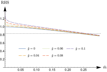
((a)) $0\leq\tilde{g}\leq 0.1$

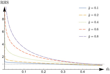
((b)) $0.1\leq\tilde{g}\leq 0.8$

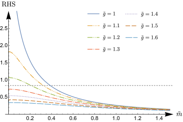
((c)) $1\leq\tilde{g}\leq 1.6$

Figure 1: Behavior of the right hand side of (34) as a function of the scaled mass $\tilde{m}$ for given ranges of the scaled coupling constant $\tilde{g}$ (curves). The constant ${2\pi^{2}}/{\tilde{G}N_{c}N_{f}}$ is plotted as a dotted line for fixed values of $G$ and $\Lambda$.

This is a central result. We note that in the limit $\tilde{g}\to 0$, that is, the limit in which the non-Hermitian term vanishes, we recover the known gap equation of the conventional Hermitian NJL model in this regularization scheme SPK ,

$$\frac{2\pi^{2}}{G\Lambda^{2}N_{c}N_{f}}=1-\frac{{m^{*}}^{2}}{\Lambda^{2}}\ln\bigg{(}1+\frac{\Lambda^{2}}{{m^{*}}^{2}}\bigg{)}.$$ (35)

In analyzing the new gap equation for the non-Hermitian NJL Hamiltonian, we choose the cutoff and the four-point interaction strength to be $\Lambda=1015$ MeV and $G\Lambda^{2}=3.93$, taking these values from the Hermitian conventional model for which $\tilde{g}=0$. We determine the solutions of the gap equation (34) from the intersection of the function given by the right hand side of the equation with the (real positive) constant on the left hand side.

Figure 1 shows the behavior of the right hand side of (34) as a function of $\tilde{m}$ for different ranges of $\tilde{g}$. This function evaluates to purely real positive values and vanishes for large values of $\tilde{m}$. In Fig. 1(a), when $\tilde{g}=0$ the right hand side of (34) takes on a finite value at $\tilde{m}=0$ and leads to the standard real solution of the conventional NJL theory. In the range $0<\tilde{g}\leq 1$ there is always a singularity at $\tilde{m}=0$, so that the gap equation has a real solution in this region, see in particular Figs. 1(a) and 1(b). However, for large values of the coupling strength $\tilde{g}>1$ the function has only a finite maximum at vanishing mass, see Fig. 1(c). We determine the height of this maximum as a function of $\tilde{g}$, see Fig. 2(a), and find that for coupling values $\tilde{g}>\tilde{g}_{\textrm{crit}}\approx 1.261$ it lies below the value of the constant given by the left hand side of (34), $2\pi^{2}/\tilde{G}N_{c}N_{f}$. Therefore, no real solution to the gap equation can be found in this region.

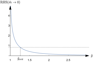
((a))

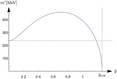
((b))

Figure 2: The behavior of the right hand side of (34) in the limit $\tilde{m}\to 0$ as a function of $\tilde{g}$ is shown in 2(a). In 2(b) the mass solution to the gap equation is shown as a function of the scaled coupling constant $\tilde{g}$.

For coupling values $1<\tilde{g}<\tilde{g}_{\textrm{crit}}$, a real solution does, however, exist and can be found again as the intersection of the right hand side of (34) with the constant on the left hand side of this equation.

The real mass solution to (34) (given in MeV) is shown in Fig. 2(b) as a function of the scaled coupling constant $\tilde{g}$. The solution starts at $m^{*}\approx 238.487$ MeV when $\tilde{g}=0$ and rises to a maximum value of $m^{*}\approx 460.870$ MeV when $\tilde{g}\approx 0.702$. Thereafter it falls to zero at $\tilde{g}_{\textrm{crit}}$ so that the solution for a particular value of the mass is doubly degenerate.

In particular, we can determine the range of scaled coupling values $\tilde{g}$ that would be necessary to generate an effective bare quark mass that corresponds to the values of the actual bare up or down quark masses. A mass solution to the gap equation that would generate a mass difference in the range of the bare up quark mass, that is $m_{u}=(1.7-3.3)$ MeV, compared to the Hermitian theory (with $\tilde{g}=0$), requires a rescaled coupling constant in the range $\tilde{g}\approx(0.025-0.034)$ or $\tilde{g}\approx(1.181-1.182)$. For the range of the bare down quark mass $m_{d}=(4.1-5.8)$ MeV we obtain the coupling range $\tilde{g}\approx(0.038-0.046)$ or $\tilde{g}\approx(1.179-1.181)$. We expect the coupling to be small, and therefore lie in the first range given.

We thus conclude that the inclusion of a non-Hermitian $\mathcal{PT}$-symmetric, chirally invariant term into the NJL Hamiltonian serves to increase the mass that is generated dynamically. That is, it can, for a certain parameter range, account for the extra small average value of $\sim 5$ MeV that is usually specified as a parameter for the bare quark mass.

III Non-Hermitian extension of the 1+1-dimensional Gross-Neveu model

The standard Gross-Neveu model is essentially the NJL model (1) defined in 1+1 dimensions, taken without isospin $\vec{\tau}$, and originally also excluding the second four-point axial interaction term. The latter version has a discrete chiral symmetry GN , while the former has this symmetry promoted to a continuous chiral symmetry. Here we can consider (1) as it stands with $\vec{\tau}$ also in 1+1 dimensions, as isospin plays a vital role in phenomenological applications. But this is simply cosmetic, as the second interaction term plays no role in the derivation of the gap equation to leading order in the $1/N_{c}$ expansion and has the same form for all these models.

Our intention is again to introduce a bilinear non-Hermitian term into the Gross-Neveu model and contrast the results obtained with those found in 3+1 dimensions. In this case, the only non-Hermitian $\mathcal{PT}$-symmetric bilinear available is $\Gamma=g\bar{\psi}\gamma_{5}\psi$. As in Sec. II we first recall the symmetry properties associated with this term within the modified free theory, before analyzing the gap equation for the fully interacting system.

III.1 Symmetries of the free theory modified by a pseudoscalar bilinear fermionic non-Hermitian terrm

In 1+1 dimensions, the only bilinear term that is non-Hermitian and $\mathcal{PT}$ symmetric is the pseudoscalar $\Gamma=g\bar{\psi}\gamma_{5}\psi$. Using the representation for the Dirac matrices AAR ,

$$\gamma^{0}=\left(\begin{array}[]{cc}0&1\\ 1&0\end{array}\right),\quad\quad\gamma^{1}=\left(\begin{array}[]{cc}0&1\\ -1&0\end{array}\right),$$

where $(\gamma^{0})^{2}=\mathbbm{1}$, $(\gamma^{1})^{2}=-\mathbbm{1}$, and $\gamma_{5}=\gamma^{0}\gamma^{1}$, we consider the modified free Hamiltonian

$$\mathcal{H}_{0}=\mathcal{H}_{F}+\Gamma=\bar{\psi}(-i\gamma^{1}\partial_{1}+m_{0}+g\gamma_{5})\psi,$$ (36)

in which $\mathcal{H}_{F}=\bar{\psi}(-i\gamma^{1}\partial_{1}+m_{0})\psi$. In addition to being non-Hermitian, $\Gamma$ also breaks the individual symmetries of parity reflection and time reversal; it is, however, invariant under the combined operations, namely, $\mathcal{PT}$ symmetry. This can be seen by studying the symmetries of the equation of motion associated with (36),

$$(i\not{\partial}-m_{0}-g\gamma_{5})\psi(t,x)=0.$$ (37)

Under a parity transformation, the spinor transforms as BKB ,

$$\mathcal{P}:\psi(t,x)\to\mathcal{P}\psi(t,x)\mathcal{P}^{-1}=\gamma^{0}\psi(t,-x),$$ (38)

and under time reversal BKB as

$$\mathcal{T}:\psi(t,x)\to\mathcal{T}\psi(t,x)\mathcal{T}^{-1}=\gamma^{0}\psi^{*}(-t,x),$$ (39)

which implies that $\mathcal{T}^{2}=+\mathbbm{1}$ for Dirac fermions in 1+1 dimensions.

Setting $x\to-x$ in (37) leads to

$$\big{(}i\gamma^{0}\partial_{0}-i\gamma^{1}\partial_{1}-m_{0}-g\gamma_{5}\big{)}\psi(t,-x)=0,$$ (40)

where $\partial_{0}=\partial_{t}$ and $\partial_{1}=\partial_{x}$ and multiplying (40) from the left by $\gamma^{0}$, we obtain

$$(i\not{\partial}-m_{0}+g\gamma_{5})\gamma^{0}\psi(t,-x)=0,$$ (41)

where we have used the fact that $\gamma^{0}$ anti-commutes with $\gamma^{1}$ and $\gamma_{5}$. From Eq. (41), one sees that the last term is odd under a parity transformation. Now letting $t\to-t$ and taking the complex conjugate of (41), we have

$$\big{[}i\gamma^{0}\partial_{0}-i\gamma^{1}\partial_{1}-m_{0}+g\gamma_{5}\big{]}\gamma^{0}\psi^{*}(-t,-x)=0.$$ (42)

By multiplying (42) from the left by $\gamma^{0}$, we establish form invariance with the original equation (37),

$$(i\not{\partial}-m_{0}-g\gamma_{5})\gamma^{0}\gamma^{0}\psi^{*}(-t,-x)=0.$$ (43)

We recognize $\gamma^{0}\gamma^{0}\psi^{*}(-t,-x)=\mathcal{PT}\psi(t,x)$. As a result, although the equation of motion is not separately invariant under parity reflection and time reversal, it remains invariant under the combined operations of $\mathcal{P}$ and $\mathcal{T}$. This fact suggests once again that the modified free non-Hermitian Hamiltonian (36) can have a real spectrum BJR . If we iterate (37), we obtain the two-dimensional Klein-Gordon equation as

$$(\partial^{2}+m_{0}^{2}-g^{2})\psi=0,$$ (44)

where we have used the fact that $\not{\partial}^{2}=\partial^{2}$. Equation (44) implies that the propagated mass is shifted by $g^{2}$, and is real and nonzero only if $m_{0}^{2}>g^{2}$.

The non-Hermitian $\mathcal{PT}$-symmetric mass term suggested here also breaks the discrete and continuous chiral symmetry explicitly, in apposition to the case in 3+1 dimensions: in the limit of vanishing bare mass $m_{0}$ (37) reads

$$(i\not{\partial}-g\gamma_{5})\psi=0.$$ (45)

Under the discrete chiral transformation $\psi\to\gamma_{5}\psi$, this becomes

$$\big{[}i\gamma^{0}\partial_{0}+i\gamma^{1}\partial_{1}-g\gamma_{5}\big{]}\gamma_{5}\psi=0,$$ (46)

which by multiplying by $\gamma_{5}$ from the left, turns into

$$(i\not{\partial}+g\gamma_{5})\psi=0,$$ (47)

where we have used the facts that $\{\gamma_{5},\gamma^{\mu}\}=0$ and $(\gamma_{5})^{2}=\mathbbm{1}$. Equation (47) shows the non-invariance of (45) under the discrete chiral transformation; similarly it is not invariant under a continuous chiral transformation where $\psi\to e^{i\alpha\gamma_{5}}\psi$ for some real $\alpha$.

III.2 The gap equation for the non-Hermitian Gross-Neveu model

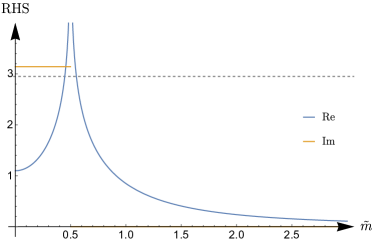
((a)) $\tilde{g}=0.5$

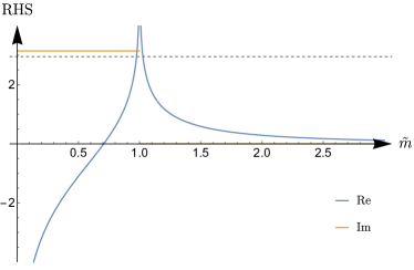
((b)) $\tilde{g}=1$

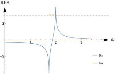
((c)) $\tilde{g}=2$

Figure 3: Behavior of the right hand side of the gap equation (57) as a function of the scaled mass $\tilde{m}$ for different values of the scaled coupling constant $\tilde{g}$.

We define the non-Hermitian Gross-Neveu model in 1+1 dimensions as

$$\mathcal{H}=\mathcal{H}_{0}-G[(\bar{\psi}\psi)^{2}+(\bar{\psi}i\gamma_{5}\vec{\tau}\psi)^{2}]=\bar{\psi}(-i\gamma^{1}\partial_{1}+m_{0}+g\gamma_{5})\psi-G[(\bar{\psi}\psi)^{2}+(\bar{\psi}i\gamma_{5}\vec{\tau}\psi)^{2}],$$ (48)

where $\mathcal{H}_{0}$ is the modified free non-Hermitian Hamiltonian in (36). The associated free propagator $S^{(0)}$ is given formally as

$$S^{(0)}(p)=(\not{p}-m_{0}-g\gamma_{5})^{-1}.$$ (49)

The arguments leading to the gap equation (20) in 3+1 dimensions are applicable here as well, so that in 1+1 dimensions, the gap equation reads

$$m^{*}=m_{0}+2iGN_{c}N_{f}\int\frac{d^{2}p}{(2\pi)^{2}}\,{\rm tr}[S(p)],$$ (50)

where the full propagator $S(p)$ has the same form as $S^{(0)}$, but with $m_{0}$ replaced by $m^{*}$. We thus proceed to evaluate the trace by expanding (49) with $(\not{p}+m_{0}+g\gamma_{5})$ and taking $m_{0}\to m^{*}$ so that the denominator becomes

$$\begin{split}&(\not{p}-m^{*}-g\gamma_{5})(\not{p}+m^{*}+g\gamma_{5})\\ &=p^{2}-m^{*}{}^{2}-g^{2}-2m^{*}g\gamma_{5}-2g\gamma_{5}\not{p},\end{split}$$ (51)

and expanding again with opposite sign in the last two terms then leads to the full propagator

$$\begin{split}&S(p)=\\ &\frac{(\not{p}+m^{*}+g\gamma_{5})[p^{2}-m^{*}{}^{2}-g^{2}+2m^{*}g\gamma_{5}+2g\gamma_{5}\not{p}]}{(p^{2}-m^{*}{}^{2}+g^{2})^{2}},\end{split}$$ (52)

with the trace

$$\mathrm{tr}[S(p)]=\frac{2m^{*}{}}{p^{2}-m^{*}{}^{2}+g^{2}}.$$ (53)

Thus, the gap equation (50) becomes

$$m^{*}=m_{0}+\frac{4iGN_{c}N_{f}m^{*}}{(2\pi)^{2}}I_{2},$$ (54)

where

$$I_{2}=\int d^{2}p\,\frac{1}{p^{2}-{m^{*}}^{2}+g^{2}}.$$ (55)

Introducing Euclidean coordinates with $p_{0}=ip_{2}$, transforming to spherical coordinates and introducing a radial cutoff $\Lambda$, $I_{2}$ becomes

$$\begin{split}I_{2}&=-i\int_{0}^{2\pi}d\theta\int_{0}^{\Lambda}dr\,\frac{r}{r^{2}+{m^{*}}^{2}-g^{2}}\\ &=-i\pi\ln\bigg{(}1+\frac{\Lambda^{2}}{{m^{*}}^{2}-g^{2}}\bigg{)}.\end{split}$$ (56)

This leads to the gap equation,

$$\frac{\pi}{GN_{c}N_{f}}=\ln\Big{(}1+\frac{1}{\tilde{m}^{2}-\tilde{g}^{2}}\Big{)},$$ (57)

in terms of the scaled mass $\tilde{m}=m^{*}/\Lambda$ and the scaled coupling constant $\tilde{g}=g/\Lambda$, in the limit of vanishing bare mass $m_{0}$. Here, we consider the case of two flavors, $N_{f}=2$, and three colors, $N_{c}=3$. We note that the four-point interaction strength in the gap equation (57) does not scale with the cutoff length $\Lambda$. This is to be expected in the 1+1-dimensional NJL model.

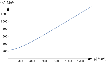
Figure 4: Visualization of the mass solution $m$ as a function of the coupling constant $g$.

In order to obtain scaled mass solutions to the gap equation that are comparable with those of the 3+1-dimensional model, we fix the four-point interaction strength $G$ such that the solution of the Hermitian theory (at $g=0$) is identical to the solution obtained there, namely $\tilde{m}=0.235$. This is achieved with $G\approx 0.177$.

The left hand side of (57) is a real positive constant and the solutions of the gap equation can be determined as the intersection of the function given by the right hand side of (57) with this constant. In Fig. 3, the behavior of this function with the scaled mass $\tilde{m}$ is shown for fixed values of the scaled coupling constant $\tilde{g}$. It visualizes the following properties of the function:

(a) The right hand side of (57) generally has two singularities, namely, one at $\tilde{m}^{2}=\tilde{g}^{2}$ and one at $\tilde{m}^{2}=\tilde{g}^{2}-1$. Inbetween, the function has complex values. As a result, the gap equation does not have real solutions in the range $\sqrt{\tilde{g}^{2}-1}\leq\tilde{m}\leq\tilde{g}$.

(b) For the special choice of coupling values $0<\tilde{g}\leq 1$, the second singularity does not occur for real masses and therefore the function has complex values for all masses in the range $0\leq\tilde{m}\leq\tilde{g}$.

(c) For coupling constants $\tilde{g}>1$ the function takes on real, but negative, values for masses lying below the first singularity, $0\leq\tilde{m}\leq\sqrt{\tilde{g}^{2}-1}$, so that an intersection with the positive constant given by the left hand side of (57) is not possible.

For mass values $\tilde{m}<\tilde{g}$, only complex solutions exist; $\mathcal{PT}$ symmetry is realized in the broken phase. For mass values $\tilde{m}>\tilde{g}$, however, the function on the right hand side of (57) generally takes on all real positive values larger than zero. Therefore, a real mass solution to the gap equation is guaranteed to exist in the region $\tilde{m}^{2}>\tilde{g}^{2}$ for all scaled coupling values $\tilde{g}$. $\mathcal{PT}$ symmetry is manifestly realized. We compare this with the analysis presented in Sec. III.1. Therein, we found that real mass solutions exist only if $m_{0}^{2}>g^{2}$ (see Eq. (44)), which implies that we are in the region of unbroken $\mathcal{PT}$ symmetry. Here, in the limit of vanishing bare mass $m_{0}$, we obtain a similar relation for the existence of the mass solutions of the gap equation.

Figure 4 shows the behavior of the solution for $m$ as function of the coupling constant $g$.

Analogous to the 3+1-dimensional model we can determine the range of the scaled coupling constant $\tilde{g}$ that gives rise to mass solutions of the gap equation which describe the range of the scaled mass $\tilde{m}$ corresponding to a current up or down quark mass in the 3+1-dimensional model. Namely, the scaled-mass range $\tilde{m}=(0.237-0.238)$, corresponding to the up quark mass in the 3+1-dimensional model, is generated by scaled coupling values in the range $\tilde{g}\approx(0.028-0.039)$. The scaled-mass range $\tilde{m}=(0.239-0.240)$, corresponding to the down quark mass in the 3+1-dimensional model, is generated by scaled coupling values in the range $\tilde{g}\approx(0.044-0.052)$.

III.3 Renormalization

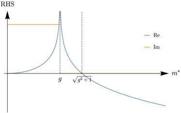
Figure 5: Behavior of the right hand side of the renormalized gap equation (60) as a function of the effective mass $m^{*}$.

Contrary to the 3+1-dimensional NJL model, the Gross-Neveu model in 1+1 dimensions is renormalizable GN . This is already indicated by the fact that the four-point interaction strength $G$ is a dimensionless parameter, see Eq. (57). Thus we can absorb the ultraviolet divergence occurring in the limit of a large cutoff $\Lambda$ into the four-point interaction strength $G$ to find the gap equation of the renormalized theory.

Introducing the arbitrary dimensionful (energy) scale $c=1$MeV writing $\Lambda=c\lambda$, with $\lambda$ dimensionless, we expand (57) in the limit $\lambda\to\infty$, yielding

$$\frac{\pi}{GN_{c}N_{f}}=2\ln\lambda+\ln\Big{(}\frac{c^{2}}{{m^{*}}^{2}-g^{2}}\Big{)}+O\Bigl{(}\frac{1}{\lambda^{2}}\Bigr{)},$$ (58)

and absorb the divergent first term on the right hand side into a renormalized four-point interaction strength $G_{R}$ defined as

$$\frac{1}{G_{R}}=\frac{1}{G}-\frac{2N_{c}N_{f}}{\pi}\ln\lambda.$$ (59)

In the limit $\lambda\to\infty$ keeping $G_{R}$ fixed, we thus obtain the renormalized gap equation

$$\frac{\pi}{G_{R}N_{c}N_{f}}=\ln\Big{(}\frac{c^{2}}{{m^{*}}^{2}-g^{2}}\Big{)}.$$ (60)

Figure 5 shows the behavior of the right hand side of (60) as a function of the effective mass $m^{*}$. This function has a singularity at $m^{*}=g$ and a root at $m^{*}=\sqrt{g^{2}+1}$. For $m^{*}<g$ the function takes on complex values and for $m^{*}>\sqrt{g^{2}+1}$ it evaluates to negative real values. In particular, all possible real mass solutions to the renormalized gap equation satisfy the relation $m^{*}>g$ since the left hand side of (60) is a real constant.

It is instructive to calculate the mass solution of (60) as a function of $g$,

$$m^{*}=\sqrt{g^{2}+c^{2}\Bigl{[}\exp\Bigl{(}\frac{\pi}{G_{R}N_{c}N_{f}}\Bigr{)}\Bigr{]}^{-1}},$$ (61)

and compare it to the scaled mass solution $\tilde{m}=m^{*}/\Lambda$ obtained from the unrenormalized gap equation (57),

$$\tilde{m}=\sqrt{\tilde{g}^{2}+\Bigl{[}\exp\Bigl{(}\frac{\pi}{GN_{c}N_{f}}\Bigr{)}-1\Bigr{]}^{-1}},$$ (62)

in terms of the scaled coupling $\tilde{g}=g/\Lambda$. In both cases the term in square brackets is a fixed positive constant determined by the value of the four-point interaction strength $G_{R}$ or $G$ respectively. When we choose the mass solution for $g=0$ to coincide with the corresponding result in the 3+1-dimensional theory the behavior of the results of the renormalized and unrenormalized systems coincide.

Figure 6 shows the general behavior of the solution (61) to the renormalized gap equation as a function of the coupling constant $g$ and the renormalized four-point interaction strength $G_{R}$. The behavior of the solution that coincides with the result of the 3+1-dimensional theory for $g=0$ is shown in red and can be compared with the solution to the unrenormalized gap equation shown in Fig. 4.

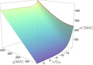
Figure 6: Behavior of the solution $m^{*}$ of the renormalized gap equation (60) as a function of the coupling constant $g$ and the renormalized four-point interaction strength $G_{R}$. The behavior of the solution that coincides with the result of the 3+1-dimensional theory for $g=0$ is shown in red.

IV Concluding remarks

$\mathcal{PT}$ symmetry is understood as the complex extension of Hermitian quantum theory BBJ . Here, we have investigated the non-Hermitian $\mathcal{PT}$-symmetric extension of the Nambu–Jona-Lasinio model in 3+1 and 1+1 dimensions, and studied the effects of these non-Hermitian terms on the process of mass generation. Our major results are the following: (1) In previous calculations for the Dirac equation that include non-Hermitian bilinear terms, contrary to expectations, no real mass spectra can be obtained in the chiral limit; a nonzero bare fermion mass is essential for the realization of $\mathcal{PT}$ symmetry in the unbroken regime. Here, in the NJL model, in which four-point interactions are present, we do find real values for the mass spectrum also in the limit of vanishing bare masses in both 3+1 and 1+1 dimensions, at least for certain specific values of the non-Hermitian couplings $g$. Thus, the four-point interaction overrides the effects leading to $\mathcal{PT}$ symmetry-breaking for these parameter values. (2) In 3+1 dimensions, we note that we are able to introduce a non-Hermitian bilinear term that preserves the chiral symmetry of the model; in 1+1 dimensions, however, the only non-Hermitian $\mathcal{PT}$-symmetric term does not possess chiral symmetry. However, in both cases, the non-Hermitian term leads to a change in the generated mass. In both models, this can be tuned to be small; we can fix the bare fermion mass to its value when $m_{0}=0$ in the absence of the non-Hermitian term, and thus determine the small generated bare fermion mass. (3) In both cases, the gap equations display a rich phase structure as a function of the coupling strengths.

References

• (1) C. M. Bender and S. Boettcher, Phys. Rev. Lett. 80, 5243 (1998).
• (2) C. M. Bender, PT Symmetry in Quantum and Classical Physics (World Scientific, Singapore, 2019).
• (3) C. M. Bender, N. Hassanpour, S. P. Klevansky, and S. Sarkar, Phys. Rev. D 98, 125003 (2018).
• (4) K. Jones-Smith and H. Mathur, Phys. Rev. A 82, 042101 (2010).
• (5) J. Alexandre, P. Millington, and D. Seynaeve, Phys. Rev. D 96, 065027 (2017).
• (6) A. Beygi, S. P. Klevansky, and R. H. Lemmer, Phys. Rev. D 101, 036005 (2020).
• (7) A. Beygi, S. P. Klevansky, and C. M. Bender, Phys. Rev. A 97, 032128 (2018).
• (8) A. Beygi and S. P. Klevansky, Phys. Rev. A 98, 022105 (2018).
• (9) A. Beygi, S. P. Klevansky, and C. M. Bender, Phys. Rev. A 99, 062117 (2019).
• (10) Y. Nambu and G. Jona-Lasinio, Phys. Rev. 122, 345 (1961).
• (11) S. P. Klevansky, Rev. Mod. Phys. 64, 649 (1992).
• (12) J. Bardeen, L. N. Cooper, and J. R. Schrieffer, Phys. Rev. 108, 1175 (1957).
• (13) A. J. Leggett, Quantum Liquids: Bose Condensation and Cooper Pairing in Condensed-Matter Systems (Oxford University Press, Oxford, 2006).
• (14) J. D. Bjorken and S. D. Drell, Relativistic Quantum Mechanics (McGraw-Hill, New York, 1965).
• (15) I. S. Gradshteyn and I. M. Ryzhik, Table of Integrals, Series, and Products, 6th ed. (Academic Press, California, 2000).
• (16) D. J. Gross and A. Neveu, Phys. Rev. D 10, 3235 (1974).
• (17) E. Abdalla, M. G. B. Abdalla, and K. D. Rothe, Non-Perturbative Methods in Two-Dimensional Quantum Field Theory (World Scientific, Singapore, 1991).
• (18) C. M. Bender, H. F. Jones, and R. J. Rivers, Phys. Lett. B 625, 333 (2005).
• (19) C. M. Bender, D. C. Brody, and H. F. Jones, Phys. Rev. Lett. 89, 270401 (2002).