Analyzing Redundancy in Pretrained Transformer Models

Abstract

Transformer-based deep NLP models are trained using hundreds of millions of parameters, limiting their applicability in computationally constrained environments. In this paper, we study the cause of these limitations by defining a notion of Redundancy, which we categorize into two classes: General Redundancy and Task-specific Redundancy. We dissect two popular pretrained models, BERT and XLNet, studying how much redundancy they exhibit at a representation-level and at a more fine-grained neuron-level. Our analysis reveals interesting insights, such as: i) 85% of the neurons across the network are redundant and ii) at least 92% of them can be removed when optimizing towards a downstream task. Based on our analysis, we present an efficient feature-based transfer learning procedure, which maintains 97% performance while using at-most 10% of the original neurons.

1 Introduction

Large pretrained models have improved the state- of-the-art in a variety of NLP tasks, with each new model introducing deeper and wider architectures causing a significant increase in the number of parameters. For example, BERT large Devlin et al. (2019), NVIDIA’s Megatron model, and Google’s T5 model Raffel et al. (2019) were trained using 340 million, 8.3 billion and 11 billion parameters respectively.

An emerging body of work shows that these models are over-parameterized and do not require all the representational power lent by the rich architectural choices during inference. For example, these models can be distilled Sanh et al. (2019); Sun et al. (2019) or pruned Voita et al. (2019); Sajjad et al. (2020), with a minor drop in performance. Recent research  Mu et al. (2018); Ethayarajh (2019) analyzed contextualized embeddings in pretrained models and showed that the representations learned within these models are highly anisotropic. While these approaches successfully exploited over-parameterization and redundancy in pretrained models, the choice of what to prune is empirically motivated and the work does not directly explore the redundancy in the network. Identifying and analyzing redundant parts of the network is useful in: i) developing a better understanding of these models, ii) guiding research on compact and efficient models, and iii) leading towards better architectural choices.

In this paper, we analyze redundancy in pretrained models. We classify it into general redundancy and task-specific redundancy. The former is defined as the redundant information present in a pretrained model irrespective of any downstream task. This redundancy is an artifact of over-parameterization and other training choices that force various parts of the models to learn similar information. The latter is motivated by pretrained models being universal feature extractors. We hypothesize that several parts of the network are specifically redundant for a given downstream task.

We study both general and task-specific redundancies at the representation-level and at a more fine-grained neuron-level. Such an analysis allows us to answer the following questions: i) how redundant are the layers within a model? ii) do all the layers add significantly diverse information? iii) do the dimensions within a hidden layer represent different facets of knowledge, or are some neurons largely redundant? iv) how much information in a pretrained model is necessary for specific downstream tasks? and v) can we exploit redundancy to enable efficiency?

We introduce several methods to analyze redundancy in the network. Specifically, for general redundancy, we use Center Kernel Alignment Kornblith et al. (2019) for layer-level analysis, and Correlation Clustering for neuron-level analysis. For task-specific redundancy, we use Linear Probing Shi et al. (2016a); Belinkov et al. (2017) to identify redundant layers, and Linguistic Correlation Analysis Dalvi et al. (2019) to examine neuron-level redundancy.

We conduct our study on two pretrained language models, BERT Devlin et al. (2019) and XLNet Yang et al. (2019). While these networks are similar in the number of parameters, they are trained using different training objectives, which accounts for interesting comparative analysis between these models. For task-specific analysis, we present our results across a wide suite of downstream tasks: four core NLP sequence labeling tasks and seven sequence classification tasks from the GLUE benchmark Wang et al. (2018). Our analysis yields the following insights:
 
General Redundancy:

• Adjacent layers are most redundant in the network, with lower layers having greater redundancy with adjacent layers.

• Up to $85\%$ of the neurons across the network are redundant in general, and can be pruned to substantially reduce the number of parameters.

• Up to $94\%$ of neuron-level redundancy is exhibited within the same or neighbouring layers.

Task-specific Redundancy:

• Layers in a network are more redundant w.r.t. core language tasks such as learning morphology as compared to sequence-level tasks.

• At least $92\%$ of the neurons are redundant with respect to a downstream task and can be pruned without any loss in task-specific performance.

• Comparing models, XLNet is more redundant than BERT.

• Our analysis guides research in model distillation and suggests preserving knowledge of lower layers and aggressive pruning of higher-layers.

Finally, motivated by our analysis, we present an efficient feature-based transfer learning procedure that exploits various types of redundancy present in the network. We first target layer-level task-specific redundancy using linear probes and reduce the number of layers required in a forward pass to extract the contextualized embeddings. We then filter out general redundant neurons present in the contextualized embeddings using Correlation Clustering. Lastly, we remove task-specific redundant neurons using Linguistic Correlation Analysis. We show that one can reduce the feature set to less than 100 neurons for several tasks while maintaining more than 97% of the performance. Our procedure achieves a speedup of up to 6.2x in computation time for sequence labeling tasks.

2 Related Work

A number of studies have analyzed representations at layer-level Conneau et al. (2018); Liu et al. (2019); Tenney et al. (2019); Kim et al. (2020); Belinkov et al. (2020) and at neuron-level Bau et al. (2019); Dalvi et al. (2019); Suau et al. (2020); Durrani et al. (2020). These studies aim at analyzing either the linguistic knowledge learned in representations and in neurons or the general importance of neurons in the model. The former is commonly done using a probing classifier Shi et al. (2016a); Belinkov et al. (2017); Hupkes et al. (2018). Recently, Voita and Titov (2020); Pimentel et al. (2020) proposed probing methods based on information theoretic measures. The general importance of neurons is mainly captured using similarity and correlation-based methods Raghu et al. (2017); Chrupała and Alishahi (2019); Wu et al. (2020). Similar to the work on analyzing deep NLP models, we analyze pretrained models at representation-level and at neuron-level. Different from them, we analyze various forms of redundancy in these models. We draw upon various techniques from the literature and adapt them to perform a redundancy analysis.

While the work on pretrained model compression Cao et al. (2020); Shen et al. (2020); Sanh et al. (2019); Turc et al. (2019); Gordon et al. (2020); Guyon and Elisseeff (2003) indirectly shows that models exhibit redundancy, little has been done to explore the redundancy in the network. Recent studies Voita et al. (2019); Michel et al. (2019); Sajjad et al. (2020); Fan et al. (2020) dropped attention heads and layers in the network with marginal degradation in performance. Their work is limited in the context of redundancy as none of the pruning choices are built upon the amount of redundancy present in different parts of the network. Our work identifies redundancy at various levels of the network and can guide the research in model compression.

3 Experimental Setup

3.1 Datasets and Tasks

To analyze the general redundancy in pre-trained models, we use the Penn Treebank development set Marcus et al. (1993), which consists of roughly 44,000 tokens. For task-specific analysis, we use two broad categories of downstream tasks – Sequence Labeling and Sequence Classification tasks. For the sequence labeling tasks, we study core linguistic tasks, i) part-of-speech (POS) tagging using the Penn TreeBank, ii) CCG super tagging using CCGBank Hockenmaier (2006), iii) semantic tagging (SEM) using Parallel Meaning Bank data Abzianidze and Bos (2017) and iv) syntactic chunking using CoNLL 2000 shared task dataset Sang and Buchholz (2000).

For sequence classification, we study tasks from the GLUE benchmark (Wang et al., 2018), namely i) sentiment analysis (SST-2) Socher et al. (2013), ii) semantic equivalence classification (MRPC) Dolan and Brockett (2005), iii) natural language inference (MNLI) Williams et al. (2018), iv) question-answering NLI (QNLI) Rajpurkar et al. (2016), iv) question pair similarity (QQP), v) textual entailment (RTE) Bentivogli et al. (2009), and vi) semantic textual similarity Cer et al. (2017). Complete statistics for all datasets is provided in Appendix A.1.

Other Settings

The neuron activations for each word in our dataset are extracted from the pre-trained model for sequence labeling while the [CLS] token’s representation (from a fine-tuned model) is used for sequence classification. The fine-tuning step is essential to optimize the [CLS] token for sentence representation. In the case of sub-words, we pick the last sub-word’s representation  Durrani et al. (2019); Liu et al. (2019). For sequence labeling tasks, we use training sets of 150K tokens, and standard development and test splits. For sequence classification tasks, we set aside $5\%$ of the training data and use it to optimize all the parameters involved in the process and report results on development sets, since the test sets are not publicly available.

3.2 Models

We present our analysis on two transformer-based pretrained models, BERT-base Devlin et al. (2019) and XLNet-base Yang et al. (2019). The former is a masked language model, while the latter is of an auto-regressive nature. We use the transformers library Wolf et al. (2019) to fine-tune these models using default hyperparameters.

Classifier Settings

For layer-level probing and neuron-level ranking, we use a logistic regression classifier with ElasticNet regularization. We train the classifier for $10$ epochs with a learning rate of $1e^{-3}$, batch size of $128$ and a value of $1e^{-5}$ for both $L1$ and $L2$ lambda regularization parameters.

4 Problem Definition

Consider a pretrained model $\mathbf{M}$ with $L$ layers: $\{l_{0},l_{1},\ldots,l_{L}\}$, where $l_{0}$ is an embedding layer and each layer $l_{i}$ is of size $H$. Given a dataset ${\mathbb{D}}=\{w_{1},w_{2},...,w_{T}\}$ consisting of $T$ words, the contextualized embedding of word $w_{j}$ at layer $l_{i}$ is ${\bm{z}}_{j}^{i}=l_{i}(w_{j})$. A neuron consists of each individual unit of ${\bm{z}}_{j}^{i}$. For example, BERT-base has $L=13$ layers, each of size 768 i.e. there are 768 individual neurons in each layer. The total number of neurons in the model are $13\times 768=9984$.

We analyze redundancy in $\mathbf{M}$ at layer-level $l_{i}$: how redundant is a layer? and at neuron-level: how redundant are the neurons? We target these two questions in the context of general redundancy and task-specific redundancy.

Notion of redundancy:

We broadly define redundancy to cover a range of observations. For example, we imply high similarity as a reflection of redundancy. Similarly, for task-specific neuron-level redundancy, we hypothesize that some neurons additionally might be irrelevant for the downstream task in hand. There, we consider irrelevancy as part of the redundancy analysis. Succinctly, two neurons are considered to be redundant if they serve the same purpose from the perspective of feature-based transfer learning for a downstream task.

5 General Redundancy

Neural networks are designed to be distributed in nature and are therefore innately redundant. Additionally, over-parameterization in pretrained models with a combination of various training and design choices causes further redundancy of information. In the following, we analyze general redundancy at layer-level and at neuron-level.

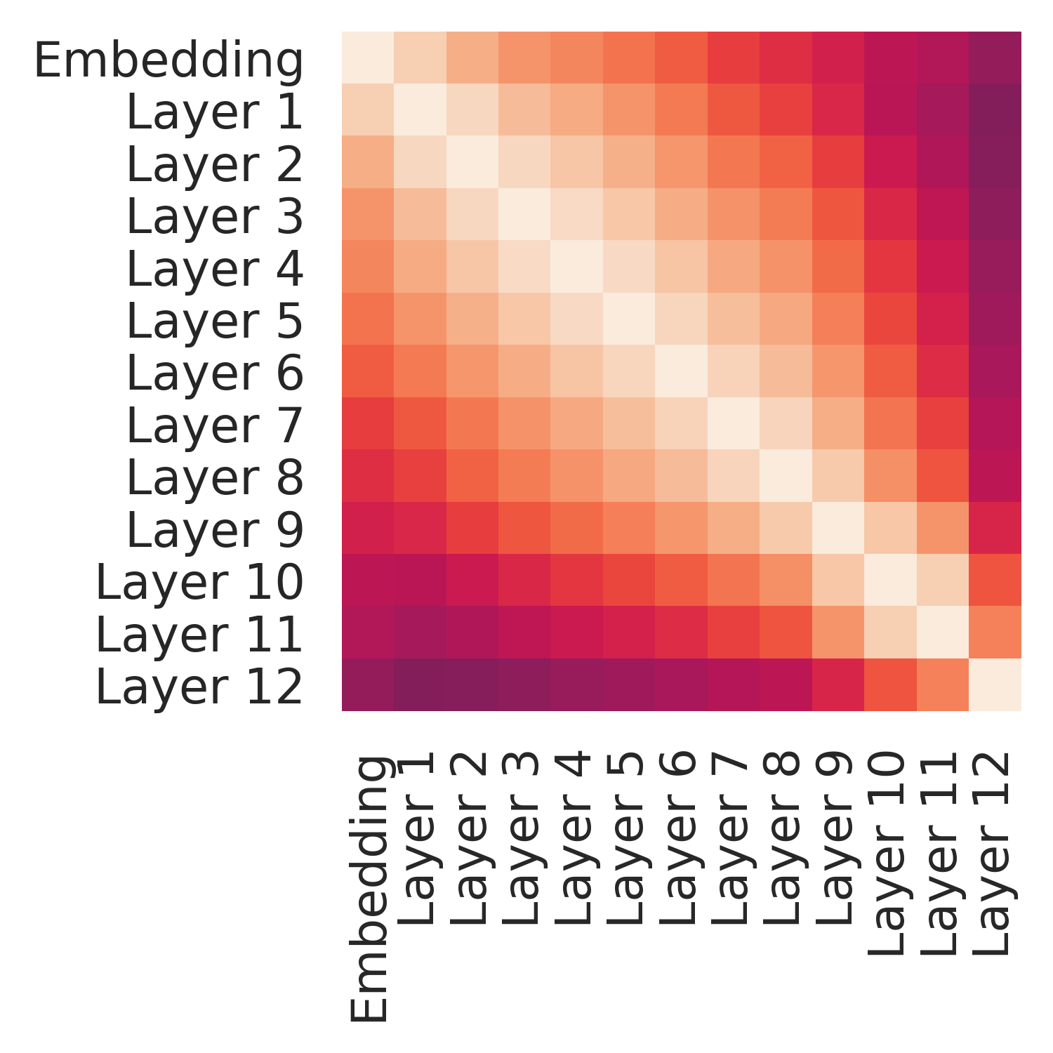
(a) BERT

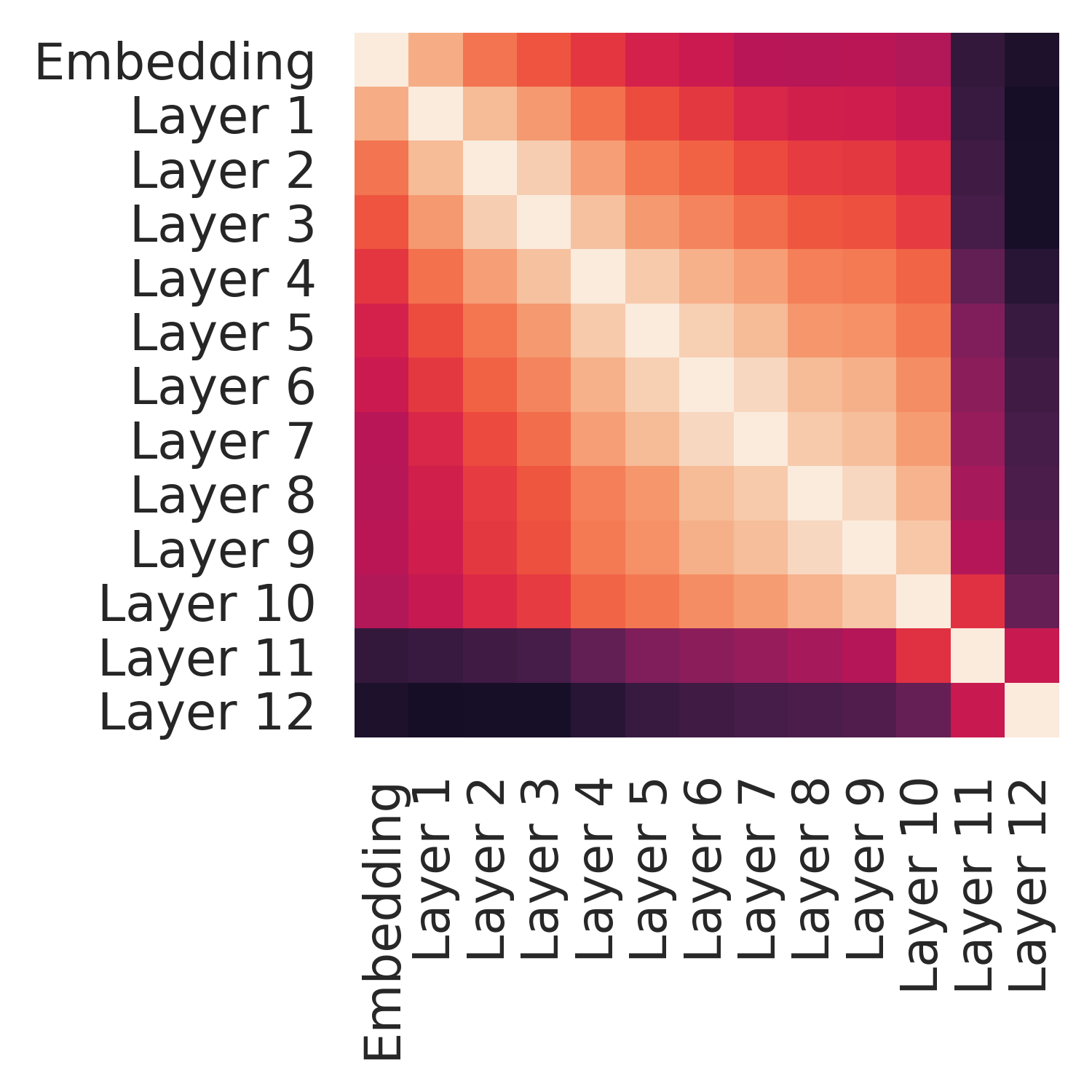
(b) XLNet

Figure 1: Pairwise Similarity between the layers. Brighter colors indicate higher similarity.

5.1 Layer-level Redundancy

We compute layer-level redundancy by comparing representations from different layers in a given model using linear Center Kernel Alignment (cka - Kornblith et al. (2019)). cka is invariant to isotropic similarity and orthogonal transformation. In other words, the similarity measure itself does not depend on the various representations having neurons or dimensions with exactly the same distributions, but rather assigns a high similarity if the two representations behave similarly over all the neurons. Moreover, cka is known to outperform other methods such as CCA Andrew et al. (2013) and SVCCA Raghu et al. (2017), in identifying relationships between different layers across different architectures. While there are several other methods proposed in literature to analyze and compare representations (Kriegeskorte et al., 2008; Bouchacourt and Baroni, 2018; Chrupała and Alishahi, 2019; Chrupała, 2019), we do not intend to compare them here and instead use cka to show redundancy in the network. The mathematical definition of cka is provided in Appendix A.6 for the reader.

We compute pairwise similarity between all $L$ layers in the pretrained model and show the corresponding heatmaps in Figure 1. We hypothesize that a high similarity entails (general) redundancy. Overall the similarity between adjacent layers is high, indicating that the change of encoded knowledge from one layer to another takes place in small incremental steps as we move from a lower layer to a higher layer. An exception to this observation is the final pair of layers, $l_{11}$ and $l_{12}$, whose similarity is much lower than other adjacent pairs of layers. We speculate that this is because the final layer is highly optimized for the objective at hand, while the lower layers try to encode as much general linguistic knowledge as possible. This has also been alluded to by others Hao et al. (2019); Wu et al. (2020).

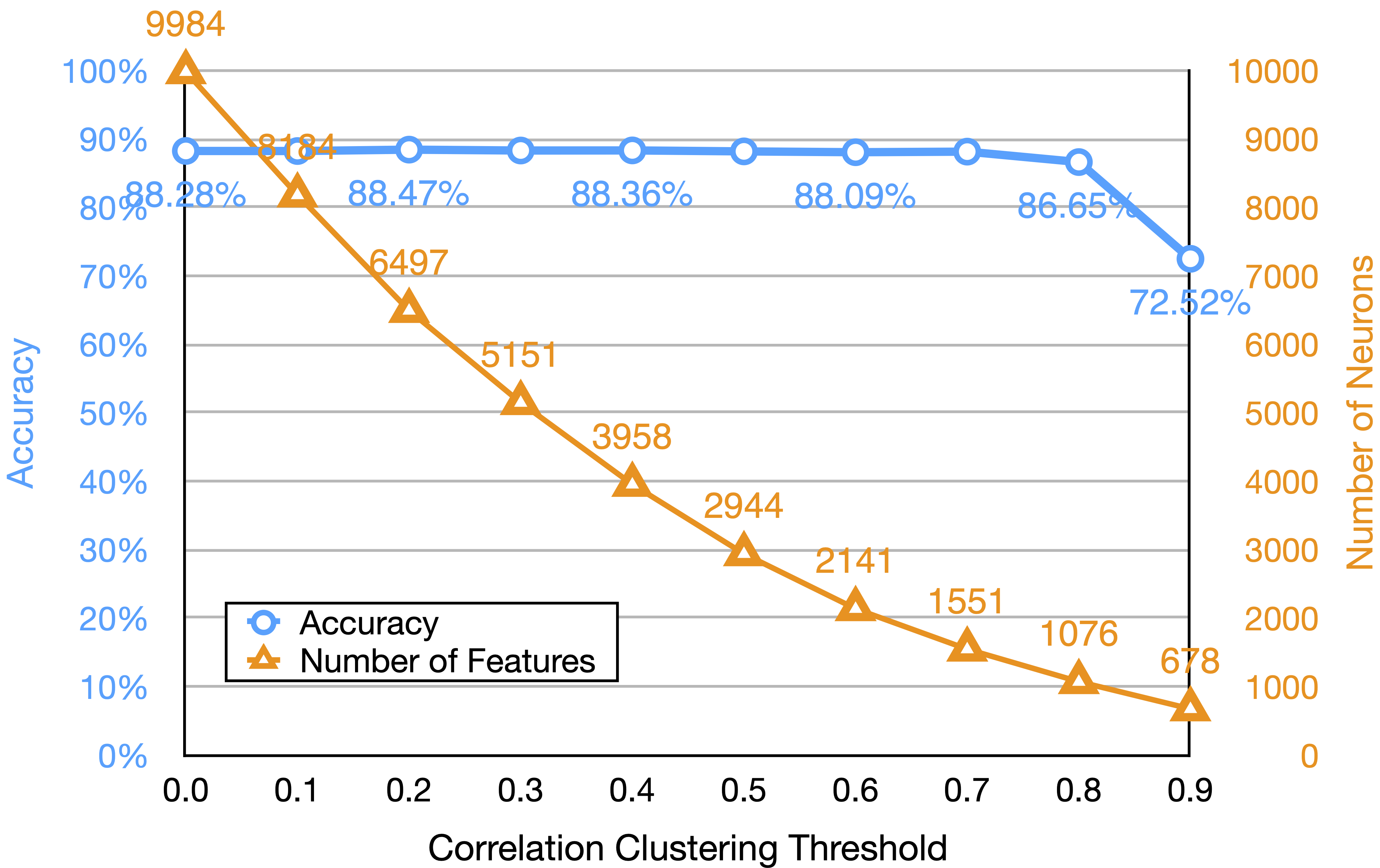
(a) BERT

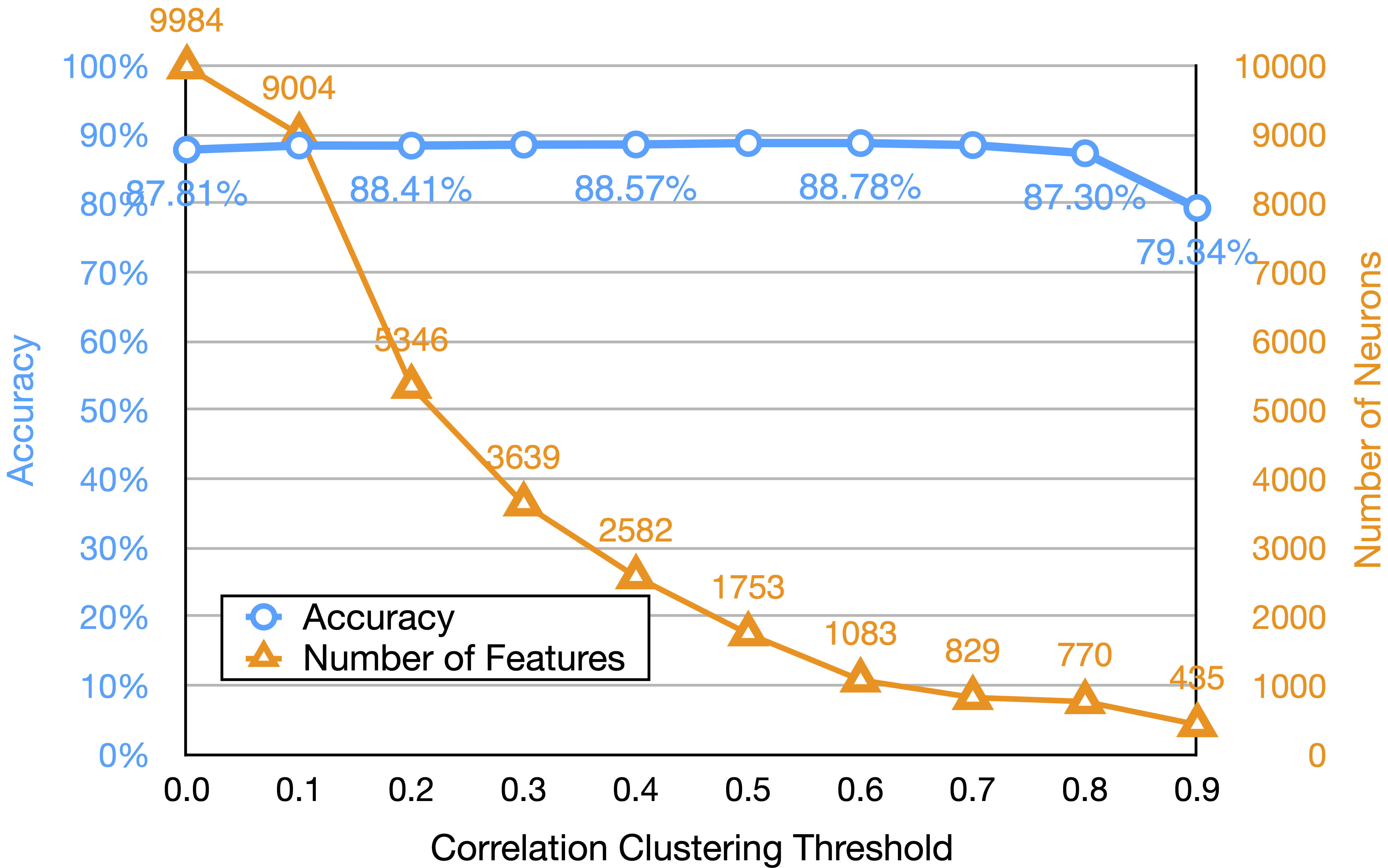
(b) XLNet

Figure 2: General neuron-level redundancy in BERT and XLNet; comparing the average reduction of neurons for different CC thresholds and the average accuracy across all downstream tasks. See Appendix A.2 for detailed per-task results.

5.2 Neuron-level Redundancy

Assessing redundancy at the layer level may be too coarse grained. Even if a layer is not redundant with other layers, a subset of its neurons may still be redundant. We analyze neuron-level redundancy in a network using correlation clustering – CC Bansal et al. (2004). We group neurons with highly correlated activation patterns over all of the words $w_{j}$. Specifically, every neuron in the vector ${\bm{z}}^{i}_{j}$ from some layer $i$ can be represented as a $T$ dimensional vector, where each index is the activation value ${\bm{z}}^{i}_{j}$ of that neuron for some word $w_{j}$, where $j$ ranges from 1 to $T$. We calculate the Pearson product-moment correlation of every neuron vector ${\bm{z}}^{i}$ with every other neuron. This results in a $N\times N$ matrix $corr$, where $N$ is the total number of neurons and $corr(x,y)$ represents the correlation between neurons $x$ and $y$. The correlation value ranges from $-1$ to $1$, giving us a relative scale to compare any two neurons. A high absolute correlation value between two neurons implies that they encode very similar information and therefore are redundant. We convert $corr$ into a distance matrix $cdist$ by applying $cdist(x,y)=1-|corr(x,y)|$ and cluster the distance matrix $cdist$ by using agglomerative hierarchical clustering with average linkage to minimize the average distance of all data points in pairs of clusters. The maximum distance between any two points in a cluster is controlled by the hyperparameter $c_{t}$. It ranges from $0$ to $1$ where a high value results in large-sized clusters with a small number of total clusters.

Figure 3: Percentage of clusters which contain neurons from the same layers, adjacent layers, within three neighboring layers and more than three layers apart.

Substantial amount of neurons are redundant

In order to evaluate the effect of clustering in combining redundant neurons, we randomly pick a neuron from each cluster and form a reduced set of non-redundant neurons. Recall that the clustering is applied independently on the data without using any task-specific labels. We then build task-specific classifiers for each task on the reduced set and analyze the average accuracy. If the average accuracy of a reduced set is close to that of the full set of neurons, we conclude that the reduced set has filtered out redundant neurons. Figure 2 shows the effect of clustering on BERT and XLNet using different values of $c_{t}$ with respect to average performance across all tasks. It is remarkable to observe that 85% of neurons can be removed without any loss in accuracy ($c_{t}=0.7$) in BERT, alluding to a high-level of neuron-level redundancy. We observe an even higher reduction in XLNet. At $c_{t}=0.7$, 92% of XLNet neurons can be removed while maintaining oracle performance. We additionally visualize a few neurons within a cluster. The activation patterns are quite similar in their behavior, though not identical, highlighting the efficacy of CC in clustering neurons with analogous behavior. An activation heatmap for several neurons is provided in Appendix A.2.

Higher neuron redundancy within and among neighboring layers

We analyze the general makeup of the clusters at $c_{t}=0.3$. Figure 3 shows the percentage of clusters that contain neurons from the same layer (window size 1), neighboring layers (window sizes 2 and 3) and from layers further apart. We can see that a vast majority of clusters ($\approx 95\%$) either contain neurons from the same layer or from adjacent layers. This reflects that the main source of redundancy is among the individual representation units in the same layer or neighboring layers of the network. The finding motivates pruning of models by compressing layers as oppose to reducing the overall depth in a distilled version of a model.

6 Task-specific Redundancy

While pretrained models have a high amount of general redundancy as shown in the previous section, they may additionally exhibit redundancies specific to a downstream task. Studying redundancy in relation to a specific task helps us understand pretrained models better. It further reflects on how much of the network, and which parts of the network, suffice to perform a task efficiently.

6.1 Layer-level Redundancy

To analyze layer-level task-specific redundancy, we train linear probing classifiers Shi et al. (2016b); Belinkov et al. (2017) on each layer $l_{i}$ (layer-classifier). We consider a classifier’s performance as a proxy for the amount of task-specific knowledge learned by a layer. Linear classifiers are a popular choice in analyzing deep NLP models due to their better interpretability Qian et al. (2016); Belinkov et al. (2020). Hewitt and Liang (2019) have shown linear probes to have higher Selectivity, a property deemed desirable for more interpretable probes.

We compare each layer-classifier with an oracle-classifier trained over concatenation of all layers of the network. For all individual layers that perform close to oracle (maintaining 99% of the performance in our results), we imply that they encode sufficient knowledge about the task and are therefore redundant in this context. Note that this does not necessarily imply that those layers are identical or that they represent the knowledge in a similar way – instead they have redundant overall knowledge specific to the task at hand.

High redundancy for core linguistic tasks

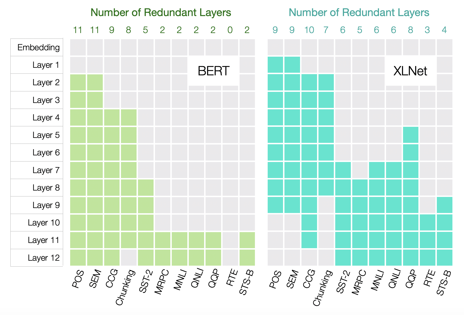
Figure 4: Task-specific layer-wise redundant layers represented by the colored blocks. Appendix A.3 presents fine-grained graphs for a few tasks.

Figure 4 shows the redundant layers that perform within a 1% performance threshold with respect to the oracle on each task. We found high layer-level redundancy for sequence labeling tasks. There are up to 11 redundant layers in BERT and up to 10 redundant layers in XLNet, across different tasks. This is expected, because the sequence labeling tasks considered here are core language tasks, and the information related to them is spread across the network. Comparing models, we found such core language information to be distributed amongst fewer layers in XLNet.

Substantially less amount of redundancy for higher-level tasks

The amount of redundancy is substantially lower for sequence classification tasks, with RTE having the least number of redundant layers in both models. Especially in BERT, we did not find any layer that matched the oracle performance for RTE. It is interesting to observe that all the sequence classification tasks are learned at higher layers and none of the lower layers were found to be redundant. These results are intuitive given that the sequence classification tasks require complex linguistic knowledge, such as long range contextual dependencies, which are only learned at the higher-layers of the model. Lower layers do not have the sufficient sentence-level context to perform these tasks well.

XLNet is more redundant than BERT

While XLNet has slightly fewer redundant layers for sequence labeling tasks, on average across all downstream tasks it shows high layer-level task-specific redundancy. Having high redundancy for sequence-level tasks reflects that XLNet learns the higher-level concepts much earlier in the network and this information is then passed to all the subsequent layers. This also showcases that XLNet is a much better candidate for model compression where several higher layers can be pruned with marginal loss in performance, as shown by Sajjad et al. (2020).

6.2 Neuron-level Redundancy

Pretrained models being a universal feature extractor contain redundant information with respect to a downstream task. We hypothesize that they may also contain information that is not necessary for the underlying task. In task-specific neuron analysis, we consider both redundant and irrelevant neurons as redundancy with respect to a task. Unlike layers, it is combinatorially intractable to exhaustively try all possible neuron permutations that can carry out a downstream task. We therefore aim at extracting only one minimal set of neurons that suffice the purpose, and consider the remaining neurons redundant or irrelevant for the task at hand.

Formally, given a task and a set of neurons from a model, we perform feature selection to identify a minimal set of neurons that match the oracle performance. To accomplish this, we use the Linguistic Correlation Analysis method Dalvi et al. (2019) to ranks neurons with respect to a downstream task, referred as FS (feature selector) henceforth. For each downstream task, we concatenate representations from all layers $L$ and use FS to extract a minimal set of top ranked neurons that maintain the oracle performance, within a defined threshold. Oracle is the task-specific classification performance obtained using all the neurons for training. The minimum set allows us to answer how many neurons are redundant and irrelevant to the given task. Tables 1 and 2 show the minimum set of top neurons for each task that maintains at least 97% of the oracle performance.

Complex core language tasks require more neurons

CCG and Chunking are relatively complex tasks compared to POS and SEM. On average across both models, these complex tasks require more neurons than POS and SEM. It is interesting to see that the size of minimum neurons set is correlated with the complexity of the task.

Task	# Neurons
POS	290
SEM	330
CCG	330
Chunk.	750

(a) BERT

Task	# Neurons
POS	280
SEM	290
CCG	690
Chunk.	660

(b) XLNet

Table 1: Task-specific neuron-level analysis for sequence labeling tasks.

Task	# Neurons
SST-2	30
MRPC	190
MNLI	30
QNLI	40
QQP	10
RTE	320
STS-B	290

(a) BERT

Task	# Neurons
SST-2	70
MRPC	170
MNLI	90
QNLI	20
QQP	20
RTE	400
STS-B	300

(b) XLNet

Table 2: Task-specific neuron-level analysis for sequence classification tasks.

Less task-specific redundancy for core linguistic tasks compared to higher-level tasks

While the minimum set of neurons per task consist of a small percentage of total neurons in the network, the core linguistic tasks require substantially more neurons compared to higher-level tasks (comparing Tables 1 and 2). It is remarkable that some sequence-level tasks require as few as only 10 neurons to obtain desired performance. One reason for the large difference in the size of minimum set of neurons could be the nature of tasks, since core linguistic tasks are word-level tasks, a much higher capacity is required in the pretrained model to store the knowledge for all of the words. While in the case of sequence classification tasks, the network learns to filter and mold the features to form fewer “high-level” sentence features.

7 Efficient Transfer Learning

In this section, we build upon the redundancy analysis presented in the previous sections and propose a novel method for efficient feature-based transfer learning. In a typical feature-based transfer learning setup, contextualized embeddings are first extracted from a pretrained model, and then a classifier is trained on the embeddings towards the downstream NLP task. The bulk of the computational expense is incurred from the following sources:

• A full forward pass over the pretrained model to extract the contextualized vector, a costly affair given the large number of parameters.

• Classifiers with large contextualized vectors are: a) cumbersome to train, b) inefficient during inference, and c) may be sub-optimal when supervised data is insufficient Hameed (2018).

We propose a three step process to target these two sources of computation bottlenecks:

1. Use the task-specific layer-classifier (Section 6.1) to select the lowest layer that maintains oracle performance. Differently from the analysis, a concatenation of all layers until the selected layer is used instead of just the individual layers.

2. Given the contextualized embeddings extracted in the previous step, use CC (Section 5.2) to filter-out redundant neurons.

3. Apply FS (Section 6.2) to select a minimal set of neurons that are needed to achieve optimum performance on the task.

The three steps explicitly target task-specific layer redundancy, general neuron redundancy and task-specific neuron redundancy respectively. We refer to Step 1 as LayerSelector (LS) and Step 2 and 3 as CCFS (Correlation clustering + Feature selection) later on. For all experiments, we use a performance threshold of 1% for LS and CCFS each. It is worth mentioning that the trade-off between loss in accuracy and efficiency can be controlled through these thresholds, which can be adjusted to serve faster turn-around or better performance.

	Sequence		Sequence
	Classification		Labeling
	BERT	XLNet	BERT	XLNet
Oracle	93.0%	93.4%	85.5%	84.8%
Neurons	9984
LS	92.3%	93.2%	85.0%	84.5%
Layers	5.3	2.5	11.6	8.1
CCFS	92.0%	92.2%	84.0%	84.0%
Neurons	425	400	90	150
% Reduct.	95.7%$\downarrow$	96.0%$\downarrow$	99.0%$\downarrow$	98.5%$\downarrow$

Table 3: Average results using LS and CCFS with performance thresholds of 1% for each. Oracle is using a concatenation of all layers. Layers shows the average number of selected layers. Neurons are the final number of neurons (features) used for classification. $\%$ Reduct. shows the percentage reduction in neurons compared to the full network.

7.1 Results

Table 3 presents the average results on all sequence labeling and sequence classification tasks. Detailed per-task results are provided in Appendix A.5.1. As expected from our analysis, a significant portion of the network can be pruned by LS for sequence labeling tasks, using less than 6 layers out of 13 (Embedding + 12 layers) for BERT and less than 3 layers for XLNet. Specifically, this reduces the parameters required for a forward pass for BERT by 65% for POS and SEM, and 33% for CCG and 39% for Chunking. On XLNet, LS led to even larger reduction in parameters; 70% for POS and SEM, and 65% for CCG and Chunking. The results were less pronounced for sequence classification tasks, with LS using 11.6 layers for BERT and 8.1 layers for XLNet on average, out of 13 layers.

Applying CCFS on top of the reduced layers led to another round of significant efficiency improvements. The number of neurons needed for the final classifier reducing to just 5% for sequence labeling tasks and 1.5% for sequence classification tasks. The final number of neurons is surprising low for some tasks compared to the initial $9984$, with some tasks like QNLI using just 10 neurons.

More concretely, taking the POS task as an example: the pre-trained oracle BERT model has 9984 features and 110M parameters. LS reduced the feature set to 2304 (embedding + 2 layers) and the number of parameters used in the forward pass to 37M. CCFS further reduced the feature set to 300, maintaining a performance close to oracle BERT’s performance on this task (95.2% vs. 93.9%).

An interesting observation in Table 3 is that the sequence labeling tasks require fewer layers but a higher number of features, while sequence classification tasks follow the opposite pattern. As we go deeper in the network, the neurons are much more richer and tuned for the task at hand, and only a few of them are required compared to the much more word-focused neurons in the lower layers. These observations suggest pyramid-shaped architectures that have wider lower layers and narrow higher layers. Such a design choice leads to significant savings of capacity in higher layers where a few, rich neurons are sufficient for good performance. In terms of neuron-based compression methods, these findings propose aggressive pruning of higher layers while preserving the lower layers in building smaller and accurate compressed models.

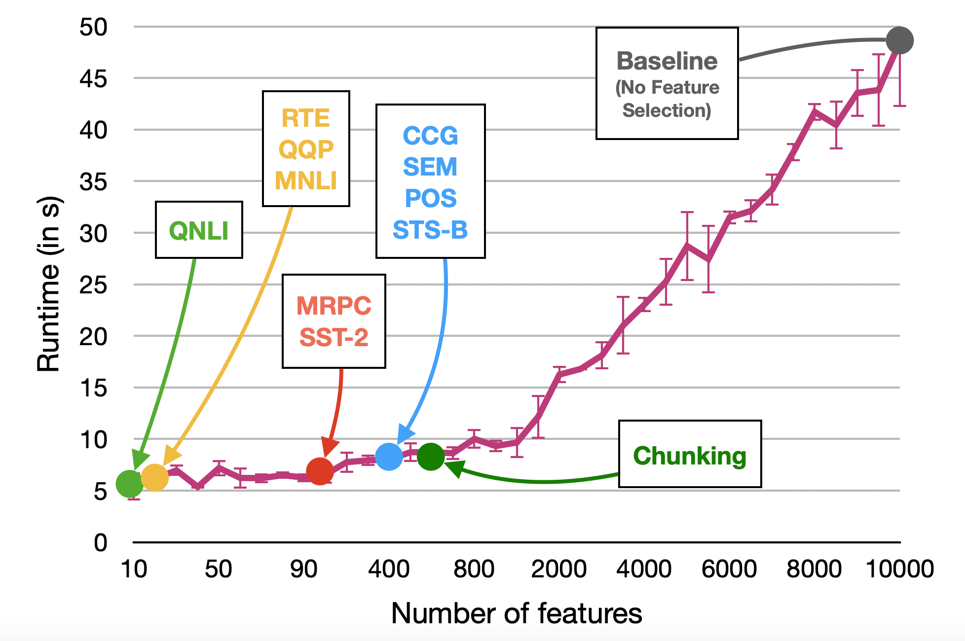
Figure 5: BERT: Runtime of the classifier w.r.t. number of neurons (features). The dots on the line mark the number of features selected by our method. Note that the X-axis is not linear, the lower half of the spectrum has been stretched for clarity.

7.2 Efficiency Analysis

While the algorithm boosts the theoretical efficiency in terms of the number of parameters reduced and the final number of features, it is important to analyze how this translates to real world performance. Using LS leads to an average speed up of $2.8{\tt x}$ and $6.2{\tt x}$ with BERT and XLNet respectively on sequence labeling tasks. On sequence classification tasks, the average speed ups are $1.1{\tt x}$ and $1.6{\tt x}$ with BERT and XLNet respectively. Detailed results are provided in Appendix A.5.2.

For the classifier built on the reduced set, we simulate a test scenario with 100,000 tokens and compute the total runtime for 10 iterations of training. The numbers were computed on a 6-core 2.8 GHz AMD Opteron Processor 4184, and were averaged across 3 runs. Figure 5 shows the runtime of each run (in seconds) against the number of features selected. The runtime of the classifier reduced from 50 to 10 seconds in the case of BERT. The $5{\tt x}$ speedup can be very useful in a heavy-use scenarios where the classifier is queried a large number times in a short duration.

Training time efficiency:

Although the focus of the current application is to improve inference-time efficiency, it is nevertheless important to understand how much computation complexity is added during training time. Let $T$ be the total number of tokens in our training set, and $N$ be the total number of neurons across all layers in a pre-trained model. The application presented in this section consists of 5 steps.

1. Feature extraction from pre-trained model: Extraction time scales linearly with the number of tokens $T$.

2. Training a classifier for every layer LS: With a constant number of neurons $N$, training time per layer scales linearly with the number of tokens $T$.

3. Correlation clustering CC: With a constant number of neurons $N$, running correlation clustering scales linearly with the number of tokens $T$.

4. Feature ranking: This step involves training a classifier with the reduced set of features, which scales linearly with the number of tokens $T$. Once the classifier is trained, the weights of the classifier are used to extract a feature ranking, with the number of weights scaling linearly with the number of selection neurons $N$.

5. Minimal feature set: Finding the minimal set of neurons is a brute-force search process, starting with a small number of neurons. For each set of neurons, a classifier is trained, the time for which scales linearly with the total number of tokens $T$. As the feature set size increases, the training time also goes up as described in Figure 5.

Appendix A.5.3 provides additional experiments and results used to analyze the training time complexity of our application.

8 Conclusion and Future Directions

We defined a notion of redundancy and analyzed pre-trained models for general redundancy and task-specific redundancy exhibited at layer-level and at individual neuron-level. Our analysis on general redundancy showed that i) adjacent layers are most redundant in the network with an exception of final layers which are close to the objective function, and ii) up to 85% and 92% neurons are redundant in BERT and XLNet respectively. We further showed that networks exhibit varying amount of task-specific redundancy; higher layer-level redundancy for core language tasks compared to sequence-level tasks. We found that at least 92% of the neurons are redundant with respect to a downstream task. Based on our analysis, we proposed an efficient transfer learning procedure that directly targets layer-level and neuron-level redundancy to achieve efficiency in feature-based transfer learning.

While our analysis is helpful in understanding pretrained models, it suggests interesting research directions towards building compact models and models with better architectural choices. For example, a high amount of neuron-level redundancy in the same layer suggests that layer-size compression might be more effective in reducing the pretrained model size while preserving oracle performance. Similarly, our finding that core-linguistic tasks are learned at lower-layers and require a higher number of neurons, while sequence-level tasks are learned at higher-layers and require fewer neurons, suggests pyramid-style architectures that have wide lower layers and compact higher layers and may result in smaller models with performance competitive with large models.

Appendix A Appendices

A.1 Data

For Sequence labeling tasks, we use the first 150,000 tokens for training, and standard development and test data for all of the four tasks (POS, SEM, CCG super tagging and Chunking). The links to all datasets is provided in the code README instructions. The statistics for the datasets are provided in Table 4.

Task	Train	Dev	Test	Tags
POS	149973	44320	47344	44
SEM	149986	112537	226426	73
Chunking	150000	44346	47372	22
CCG	149990	45396	55353	1272

Table 4: Data statistics (number of tokens) on training, development and test sets used in the experiments and the number of tags to be predicted

For the sequence classification tasks, we study tasks from the GLUE benchmark (Wang et al., 2018), namely i) sentiment analysis (SST-2) using the Stanford sentiment treebank Socher et al. (2013), ii) semantic equivalence classification using the Microsoft Research paraphrase corpus (MRPC) Dolan and Brockett (2005), iii) natural language inference corpus (MNLI) Williams et al. (2018), iv) question-answering NLI (QNLI) using the SQUAD dataset Rajpurkar et al. (2016), iv) question pair similarity using the Quora Question Pairs dataset (QQP), v) textual entailment using recognizing textual entailment dataset(RTE) Bentivogli et al. (2009), and vi) semantic textual similarity using the STS-B dataset Cer et al. (2017). The statistics for the datasets are provided in Table 5.

Task	Train	Dev
SST-2	67349	872
MRPC	3668	408
MNLI	392702	9815
QNLI	104743	5463
QQP	363846	40430
RTE	2490	277
STS-B	5749	1500

Table 5: Data statistics (number of sequences) on the official training and development sets used in the experiments. All tasks are binary classification tasks, except for STS-B which is a regression task. Recall that the test sets are not publicly available, and hence we use 10% of the official train as development, and the official development set as our test set. Exact split information is provided in the code README.

A.2 General Neuron-level Redundancy

Table 6 presents the detailed results for the illustration in Figures 2(a) and 2(b). As a concrete example, 6 out of 12 tasks (POS, SEM, CCG, Chunking, SST-2, STS-B) can do away with more than $85\%$ reduction in the number of neurons (threshold=0.7) with very little loss in performance.

Figure 6 visualizes heatmaps of a few neurons that belong to the same cluster built using CC at $c_{t}=0.3$ as a qualitative example of a cluster.

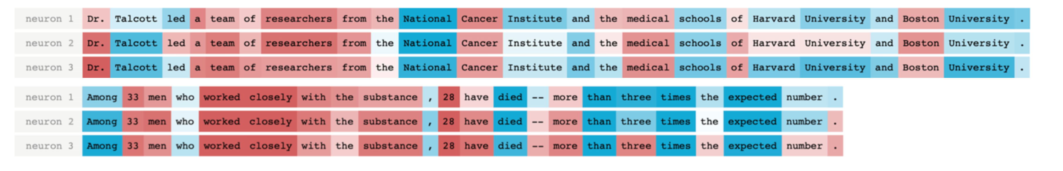
Figure 6: Redundant neurons as clustered by correlation clustering on two sentences. The dark red and dark blue refer to high negative and positive activation values respectively.

Threshold	POS	SEM	CCG	Chunking	SST-2	MRPC	MNLI	QNLI	QQP	RTE	STS-B	Average
0.0	9984	9984	9984	9984	9984	9984	9984	9984	9984	9984	9984	9984
0.0	95.7%	92.0%	89.8%	94.5%	90.5%	85.8%	81.7%	90.3%	91.2%	70.0%	89.5%	88.3%
0.1	6841	6809	6844	6749	7415	9441	9398	8525	8993	9647	8129	8072
0.1	95.4%	92.3%	90.3%	94.8%	89.8%	86.3%	81.7%	90.2%	91.2%	69.3%	89.7%	88.3%
0.2	4044	4045	4052	4008	6207	8486	8376	7225	7697	8705	6377	6293
0.2	95.9%	92.9%	90.6%	95.0%	90.6%	86.8%	81.7%	90.1%	91.2%	69.0%	89.6%	88.5%
0.3	2556	2566	2570	2573	4994	7328	7049	6131	6413	7157	4949	4935
0.3	96.2%	93.1%	91.3%	95.1%	90.6%	86.0%	81.8%	89.9%	91.1%	67.1%	89.5%	88.3%
0.4	1729	1752	1729	1709	3812	5779	5681	4961	5077	5587	3674	3772
0.4	96.2%	93.3%	91.4%	95.2%	90.4%	86.5%	81.7%	89.4%	91.0%	67.5%	89.3%	88.4%
0.5	1215	1190	1221	1217	2746	4420	4289	3747	3789	4241	2721	2800
0.5	96.4%	93.2%	91.6%	94.9%	90.3%	86.3%	81.6%	89.6%	91.1%	66.4%	89.0%	88.2%
0.6	876	869	873	876	1962	3287	3041	2712	2767	3170	1962	2036
0.6	96.2%	93.3%	91.5%	94.4%	90.0%	85.5%	81.8%	89.7%	91.1%	66.8%	88.8%	88.1%
0.7	792	789	792	795	1404	2258	2025	1867	1907	2315	1419	1488
0.7	96.2%	93.2%	91.6%	94.1%	89.8%	86.3%	81.7%	89.3%	91.1%	69.0%	87.8%	88.2%
0.8	764	758	762	748	982	1367	1239	1191	1226	1531	982	1050
0.8	96.1%	93.2%	91.3%	94.0%	89.2%	85.0%	80.6%	88.3%	90.0%	62.8%	82.6%	86.7%
0.9	443	378	429	357	778	812	798	797	814	854	785	659
0.9	95.6%	91.8%	89.9%	91.0%	56.5%	70.3%	53.2%	80.0%	77.6%	59.2%	32.5%	72.5%

(a) BERT

Threshold	POS	SEM	CCG	Chunking	SST-2	MRPC	MNLI	QNLI	QQP	RTE	STS-B	Average
0.0	9984	9984	9984	9984	9984	9984	9984	9984	9984	9984	9984	9984
0.0	96.2%	91.8%	90.6%	93.5%	93.2%	86.5%	78.9%	89.1%	87.4%	69.7%	89.0%	87.8%
0.1	9019	9021	9046	8941	7435	9206	7913	8056	5844	9931	9125	9006.75
0.1	96.3%	92.2%	90.7%	93.9%	93.0%	86.5%	80.3%	89.2%	89.7%	71.8%	89.0%	88.4%
0.2	5338	5392	5346	5302	6257	7685	6668	7393	4952	9244	8011	5344.5
0.2	96.2%	92.3%	90.5%	93.9%	93.0%	86.8%	80.4%	89.9%	90.2%	70.4%	88.9%	88.4%
0.3	3646	3651	3660	3606	5206	6241	5988	6613	4482	7635	6407	3640.75
0.3	96.2%	92.5%	91.0%	93.8%	92.9%	86.8%	80.8%	89.8%	90.1%	71.5%	88.7%	88.5%
0.4	2592	2571	2599	2573	4181	4896	5252	5583	3987	5996	4932	2583.75
0.4	96.3%	92.7%	90.8%	93.7%	93.1%	88.0%	81.0%	89.7%	90.1%	70.4%	88.5%	88.6%
0.5	1754	1746	1756	1758	3207	3675	4172	4426	3271	4573	3669	1753.5
0.5	96.5%	92.8%	91.3%	94.4%	93.2%	87.7%	80.8%	89.6%	90.1%	71.8%	88.3%	88.8%
0.6	1090	1085	1091	1072	2355	2549	2905	3248	2370	3346	2666	1084.5
0.6	96.7%	93.0%	91.8%	93.8%	93.1%	88.0%	81.0%	90.4%	90.0%	70.4%	88.4%	88.8%
0.7	833	833	830	824	1663	1735	1883	2224	1627	2348	1859	830
0.7	96.6%	93.0%	91.9%	93.2%	92.0%	88.2%	79.9%	90.1%	89.7%	71.1%	87.7%	88.5%
0.8	773	775	773	762	1127	1108	1189	1399	1091	1469	1232	770.75
0.8	96.5%	92.9%	91.9%	93.0%	92.4%	85.5%	77.3%	89.4%	87.4%	69.3%	84.5%	87.3%
0.9	470	412	471	414	799	790	805	839	791	832	801	441.75
0.9	96.0%	91.5%	91.0%	90.5%	84.4%	75.0%	65.8%	79.7%	88.3%	63.9%	46.6%	79.3%

(b) XLNet

Table 6: Accuracies and number of neurons across all tasks after running correlation clustering. Recall that the clustering is run without any task specific labels, and the evaluation is done across all tasks to analyze the efficacy of correlation clustering as a method to remove redundant neurons.

A.3 Task-Specific Layer-wise redundancy

Tables 7(a) and 7(a) provide detailed results used to produce the illustrations in Figure 4.

Figures 7, 8 and 9 show the layer-wise task-specific redundancy for individual classes within POS, SEM and Chunking respectively. We do not present these fine-grained plots for CCG (over 1000 classes) or sequence classification tasks (binary classification only).

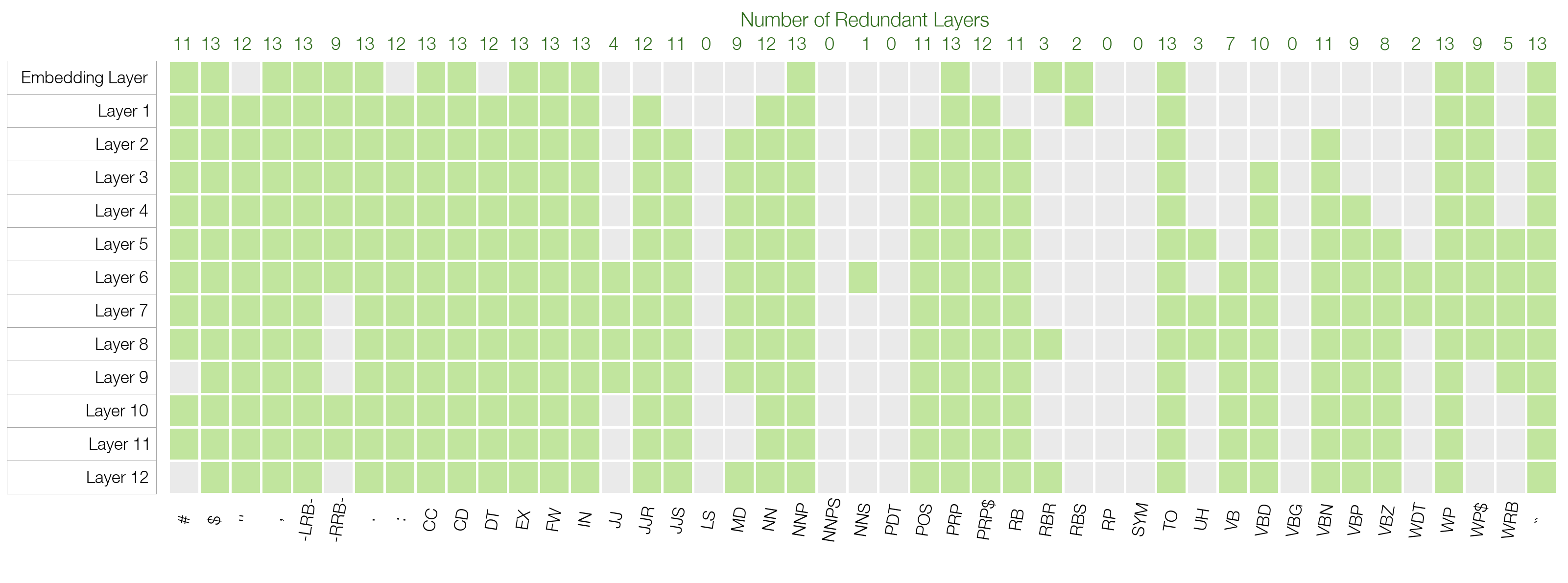
(a) BERT

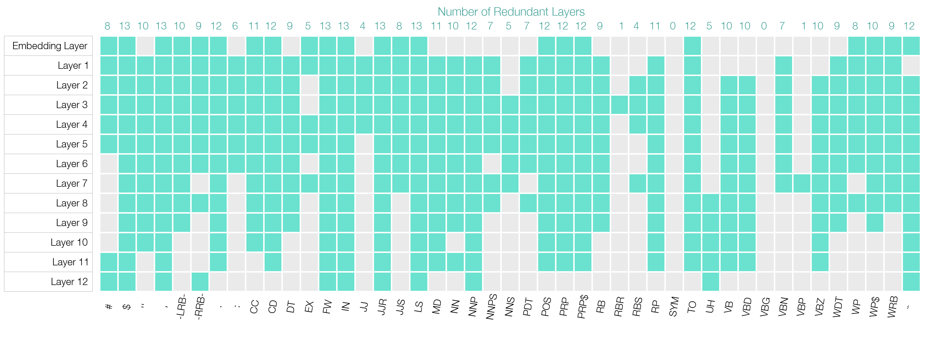
(b) XLNet

Figure 7: Layer-wise task specific redudancy for POS task. Redundant layers are represented by the colored blocks.

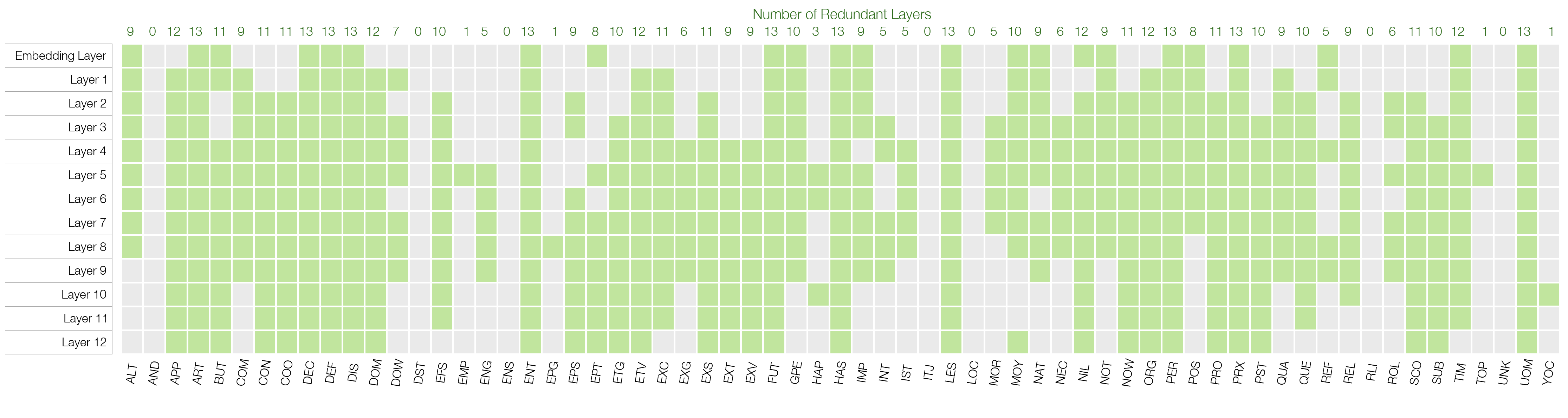
(a) BERT

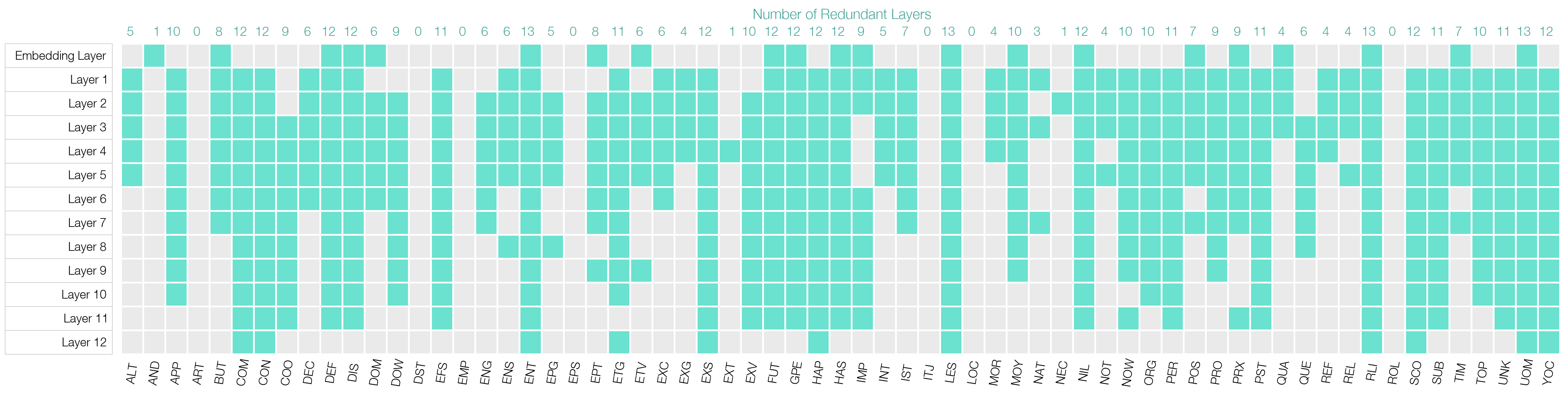
(b) XLNet

Figure 8: Layer-wise task specific redudancy for SEM task. Redundant layers are represented by the colored blocks.

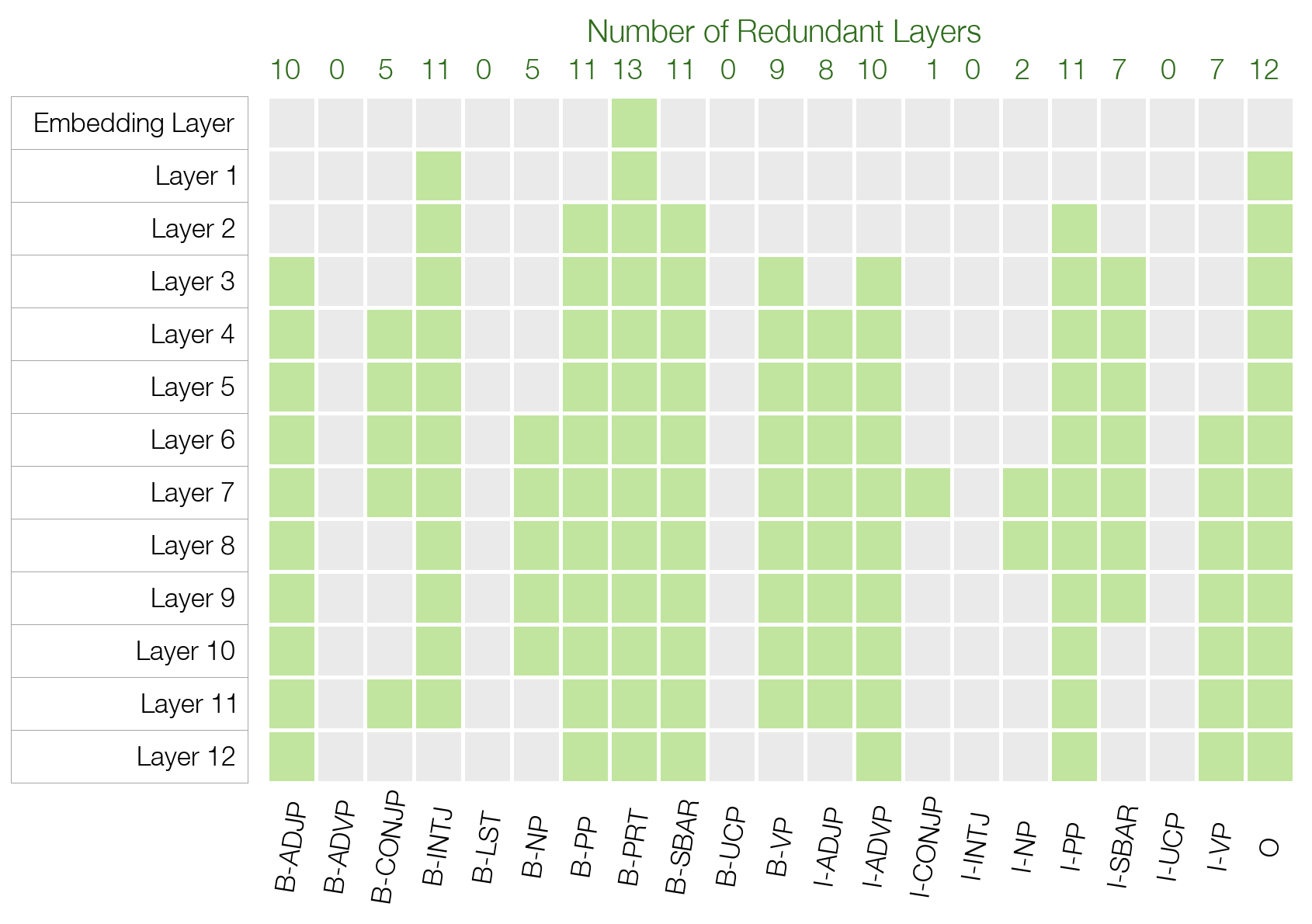
(a) BERT

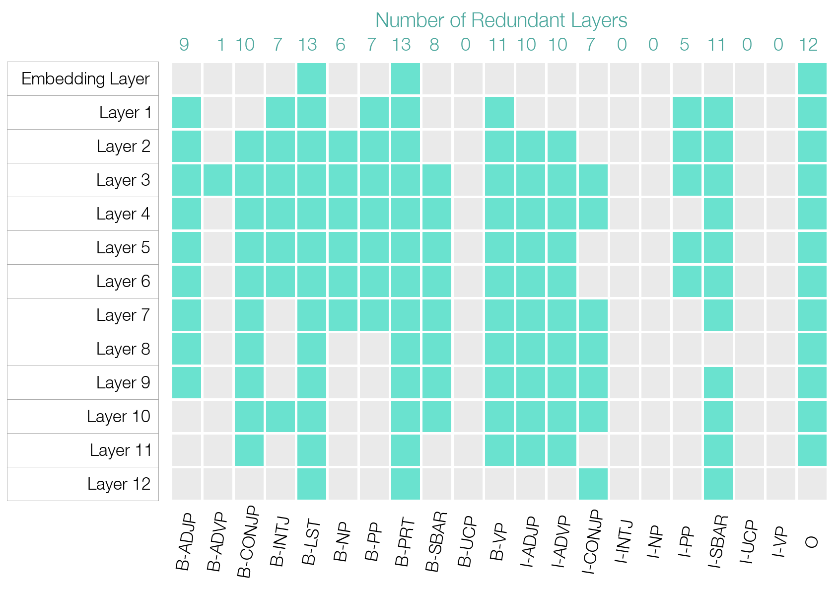
(b) XLNet

Figure 9: Layer-wise task specific redudancy for Chunking task. Redundant layers are represented by the colored blocks.

	POS	SEM	CCG	Chunking	SST-2	MRPC	MNLI	QNLI	QQP	RTE	STS-B
Oracle	95.2%	92.0%	90.1%	94.6%	90.6%	86.0%	81.7%	90.2%	91.2%	69.3%	89.7%
1% Loss	94.2%	91.1%	89.2%	93.6%	89.7%	85.2%	80.9%	89.3%	90.2%	68.6%	88.8%
Embedding	89.6%	81.5%	70.0%	77.5%	50.9%	68.4%	31.8%	49.5%	63.2%	52.7%	0.0%
Layer 1	93.1%	87.6%	78.9%	82.1%	78.4%	68.9%	42.8%	59.7%	71.4%	52.7%	6.0%
Layer 2	95.3%	91.7%	86.6%	91.0%	80.2%	71.3%	45.0%	61.2%	73.3%	56.0%	10.4%
Layer 3	95.5%	92.3%	88.0%	92.0%	80.6%	69.6%	54.0%	74.4%	77.2%	54.9%	54.5%
Layer 4	96.0%	93.0%	89.6%	94.0%	81.2%	75.5%	61.8%	81.3%	80.1%	55.6%	84.9%
Layer 5	96.0%	93.2%	90.4%	94.0%	82.3%	76.2%	65.9%	82.9%	84.4%	59.6%	85.8%
Layer 6	96.3%	93.4%	91.6%	94.9%	86.2%	77.5%	71.6%	83.2%	85.8%	62.1%	86.4%
Layer 7	96.2%	93.3%	91.9%	95.1%	88.6%	79.4%	74.9%	83.8%	86.9%	62.5%	86.8%
Layer 8	96.0%	93.1%	91.9%	94.8%	90.6%	77.5%	76.4%	84.4%	87.1%	63.5%	87.1%
Layer 9	95.8%	92.9%	91.6%	94.5%	90.5%	83.3%	79.8%	84.8%	87.7%	63.2%	87.0%
Layer 10	95.6%	92.5%	91.2%	94.1%	90.6%	82.6%	80.3%	86.1%	89.0%	64.3%	87.3%
Layer 11	95.4%	92.3%	90.9%	93.9%	90.4%	85.8%	81.7%	89.8%	91.0%	66.4%	88.9%
Layer 12	95.1%	92.0%	90.2%	93.2%	90.1%	87.3%	82.0%	90.4%	91.1%	66.1%	89.7%

(a) BERT

	POS	SEM	CCG	Chunking	SST-2	MRPC	MNLI	QNLI	QQP	RTE	STS-B
Oracle	95.9%	92.5%	90.8%	94.2%	92.4%	86.5%	78.9%	88.7%	87.2%	71.1%	88.9%
1% Loss	95.0%	91.5%	89.9%	93.3%	91.5%	85.7%	78.1%	87.8%	86.4%	70.4%	88.0%
Embedding	89.5%	82.6%	70.5%	77.0%	50.9%	68.4%	32.7%	50.5%	63.2%	52.7%	0.6%
Layer 1	96.3%	92.9%	88.7%	90.8%	79.6%	70.6%	44.2%	58.9%	72.0%	47.3%	8.8%
Layer 2	96.7%	93.6%	91.0%	93.4%	81.1%	70.1%	45.1%	58.6%	73.8%	45.8%	11.0%
Layer 3	96.8%	93.5%	91.8%	94.2%	84.7%	71.1%	61.6%	74.2%	82.4%	47.3%	81.1%
Layer 4	96.7%	93.4%	92.1%	94.2%	88.3%	76.0%	63.7%	74.1%	85.0%	53.1%	82.8%
Layer 5	96.6%	93.2%	92.4%	93.9%	88.6%	79.4%	68.4%	81.3%	89.2%	62.1%	84.9%
Layer 6	96.3%	92.6%	92.0%	94.2%	90.1%	83.1%	73.9%	83.3%	89.9%	63.5%	85.9%
Layer 7	96.1%	92.3%	91.9%	94.0%	92.9%	85.3%	79.1%	88.1%	89.9%	67.1%	86.7%
Layer 8	95.8%	91.9%	91.6%	93.5%	93.6%	87.7%	80.7%	90.0%	89.2%	65.0%	87.6%
Layer 9	95.3%	91.6%	91.4%	93.1%	94.2%	87.5%	80.1%	90.3%	88.4%	69.3%	88.2%
Layer 10	94.9%	91.2%	90.8%	92.1%	93.8%	86.5%	80.1%	90.4%	88.9%	71.8%	88.2%
Layer 11	94.6%	90.8%	90.2%	91.1%	94.5%	86.8%	80.1%	90.5%	88.5%	71.8%	88.5%
Layer 12	92.0%	87.4%	86.0%	85.9%	93.8%	86.5%	80.8%	90.6%	89.3%	71.1%	88.5%

(b) XLNet

Table 7: Task specific layer wise results across all tasks. The oracle is trained on all 13 layers combined. Bold numbers highlight layers for each task that maintain 99% of the Oracle’s performance

A.4 Task-Specific Neuron-level Redundancy

Tables 8(a) and 8(b) provide the per-task detailed results along with reduced accuracies after running task-specific neuron-level redundancy analysis.

Task	Oracle	#Neurons	Reduced Accuracy
POS	95.7%	290	94.3%
SEM	92.2%	330	90.8%
CCG	89.9%	330	88.7%
Chunking	94.4%	750	93.8%
Word Average	93.1%	425	91.9%
SST-2	90.6%	30	88.4%
MRPC	86.3%	190	85.0%
MNLI	81.7%	30	81.8%
QNLI	90.3%	40	89.1%
QQP	91.2%	10	90.8%
RTE	69.7%	320	68.6%
STS-B	89.6%	290	88.3%
Sentence Average	85.6%	130	84.6%

(a) BERT

Task	Oracle	#Neurons	Reduced Accuracy
POS	96.1%	280	95.6%
SEM	92.2%	290	91.1%
CCG	90.2%	690	89.8%
Chunking	94.1%	660	93.0%
Word Average	93.2%	480	92.4%
SST-2	92.9%	70	91.3%
MRPC	85.8%	170	85.0%
MNLI	79.0%	90	77.9%
QNLI	88.3%	20	88.5%
QQP	87.4%	20	88.0%
RTE	70.4%	400	71.1%
STS-B	88.9%	300	86.6%
Sentence Average	84.7%	152	84.1%

(b) XLNet

Table 8: Accuracies after running linguistic correlation analysis and extracting the minimal set of neurons from all 9984 neurons

A.5 Application: Efficient Feature Selection

A.5.1 Transfer Learning Detailed Results

Tables 9 and 10 show the detailed per-task results for our proposed feature selection algorithm.

		POS	SEM	CCG	Chunking
BERT	Oracle	95.2%	92.0%	90.1%	94.6%
	Neurons	9984
	LS	94.8%	91.2%	89.2%	94.0%
	Layers	3	3	8	7
	CCFS	93.9%	90.1%	90.2%	93.7%
	Neurons	300	400	400	600
	% Reduct.	97%$\downarrow$	96%$\downarrow$	96%$\downarrow$	94%$\downarrow$
XLNet	Oracle	95.9%	92.5%	90.8%	94.2%
	Neurons	9984
	LS	96.3%	92.9%	90.3%	93.5%
	Layers	2	2	3	3
	CCFS	95.6%	91.9%	89.5%	91.8%
	Neurons	300	400	300	600
	% Reduct.	97%$\downarrow$	96%$\downarrow$	97%$\downarrow$	94%$\downarrow$

Table 9: Results of sequence labeling tasks using LayerSelector(LS) with performance threshold$=1$ and CCFS with performance threshold$=1$. Oracle is using a concatenation of all layers. Layers shows the number of the selected layer. Neurons are the final number of neurons (features) used for classification. $\%$ Reduct. shows the percentage reduction in neurons compared to the full network.

		SST-2	MRPC	MNLI	QNLI	QQP	RTE	STS-B
BERT	Oracle	90.6%	86.0%	81.7%	90.2%	91.2%	69.3%	89.7%
	Neurons	9984
	LS	88.2%	86.0%	81.6%	89.9%	90.9%	69.3%	89.1%
	Layers	8	12	12	12	12	13	12
	CCFS	87.0%	86.3%	81.3%	89.1%	89.9%	65.7%	88.6%
	Neurons	30	100	30	10	20	30	400
	% Reduction	99.7%$\downarrow$	99.0%$\downarrow$	99.7%$\downarrow$	99.9%$\downarrow$	99.8%$\downarrow$	99.9%$\downarrow$	96.0%$\downarrow$
XLNet	Oracle	92.4%	86.5%	78.9%	88.7%	87.2%	71.1%	88.9%
	Neurons	9984
	LS	88.2%	86.0%	79.9%	88.8%	89.3%	71.1%	88.1%
	Layers	6	9	8	8	6	11	9
	CCFS	87.5%	89.0%	78.4%	88.3%	88.8%	69.0%	87.2%
	Neurons	50	100	50	200	100	100	400
	% Reduction	99.5%$\downarrow$	99.0%$\downarrow$	99.5%$\downarrow$	98.0%$\downarrow$	99.0%$\downarrow$	99.0%$\downarrow$	96.0%$\downarrow$

Table 10: Results of sequence classification tasks using LayerSelector(LS) with performance threshold$=1$ and CCFS with performance threshold$=1$. Oracle is using a concatenation of all layers. Layers shows the number of the selected layer. Neurons are the final number of neurons (features) used for classification. $\%$ Reduct. shows the percentage reduction in neurons compared to the full network.

A.5.2 Pretrained model timing analysis

The average runtime per instance was computed by dividing the total number of seconds taken to run the forward pass for all batches by the total number of sentences. All computation was done on an NVidia GeForce GTX TITAN X, and the numbers are averaged across 3 runs. Figures 10 and 11 shows the results of various number of layers (with the selected layer highlighted for each task).

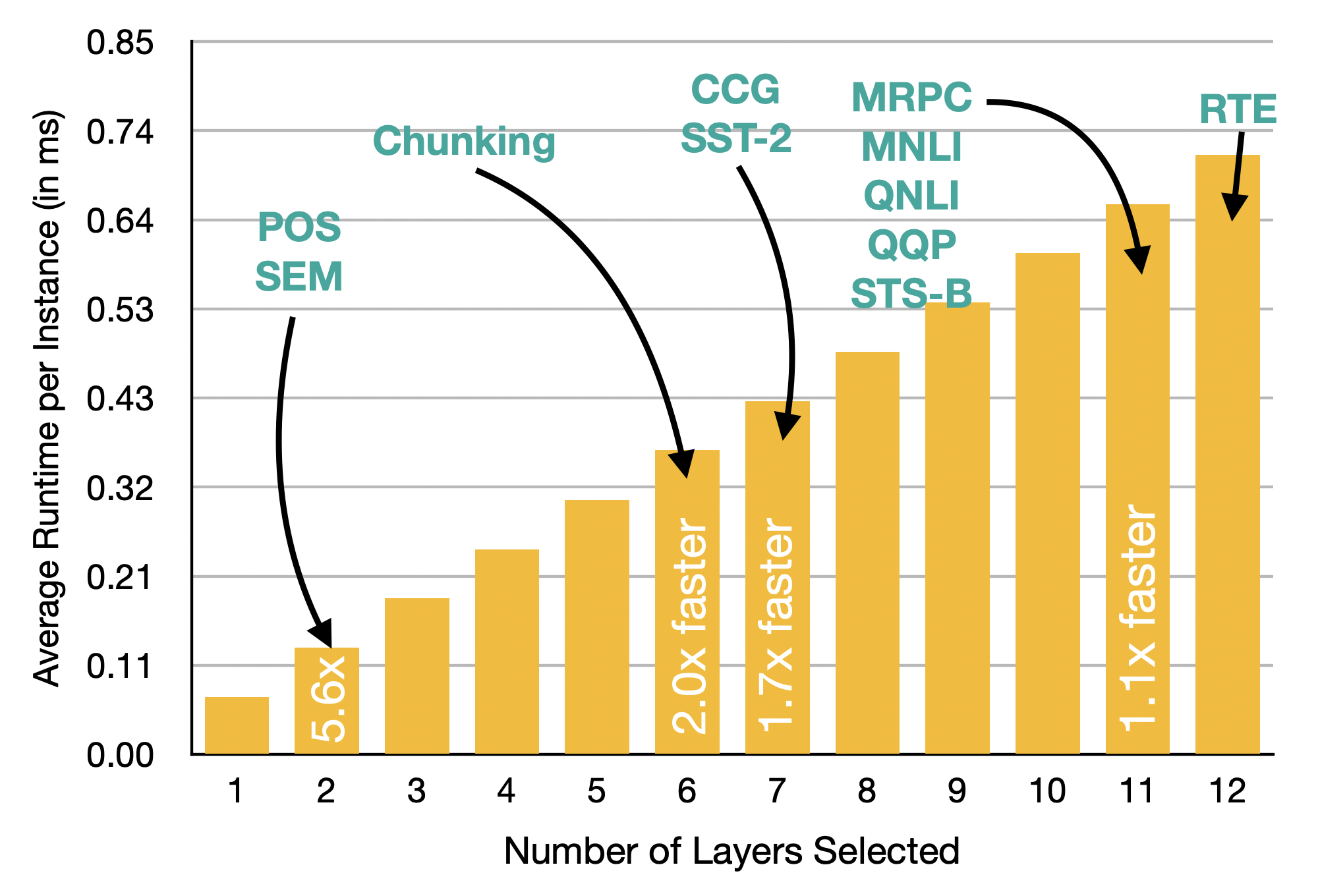
Figure 10: Average runtime per instance computed across all sequence classification tasks for BERT. Sequence classification tasks all have a near $2{\tt x}$ speed up, while most sequence labeling tasks have a $1.08{\tt x}$ speedup.

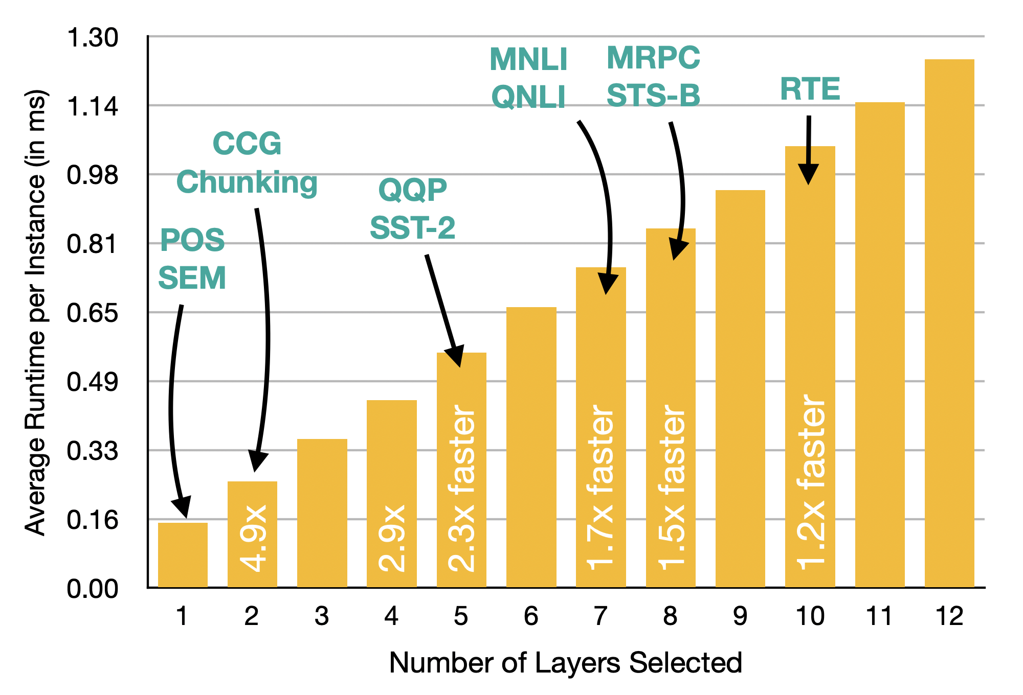
Figure 11: Average runtime per instance computed across all sequence classification tasks for XLNet. Sequence classification tasks all have a near $2{\tt x}$ speed up, while most sequence labeling tasks have a $1.08{\tt x}$ speedup.

A.5.3 Training time analysis

Figures 12, 13 and 14 show the runtimes of the various steps of the proposed efficient feature selection for transfer learning application. Extraction of features and correlation clustering both scale linearly as the number of input tokens increases, while ranking the various features scales linearly with the number of total features.

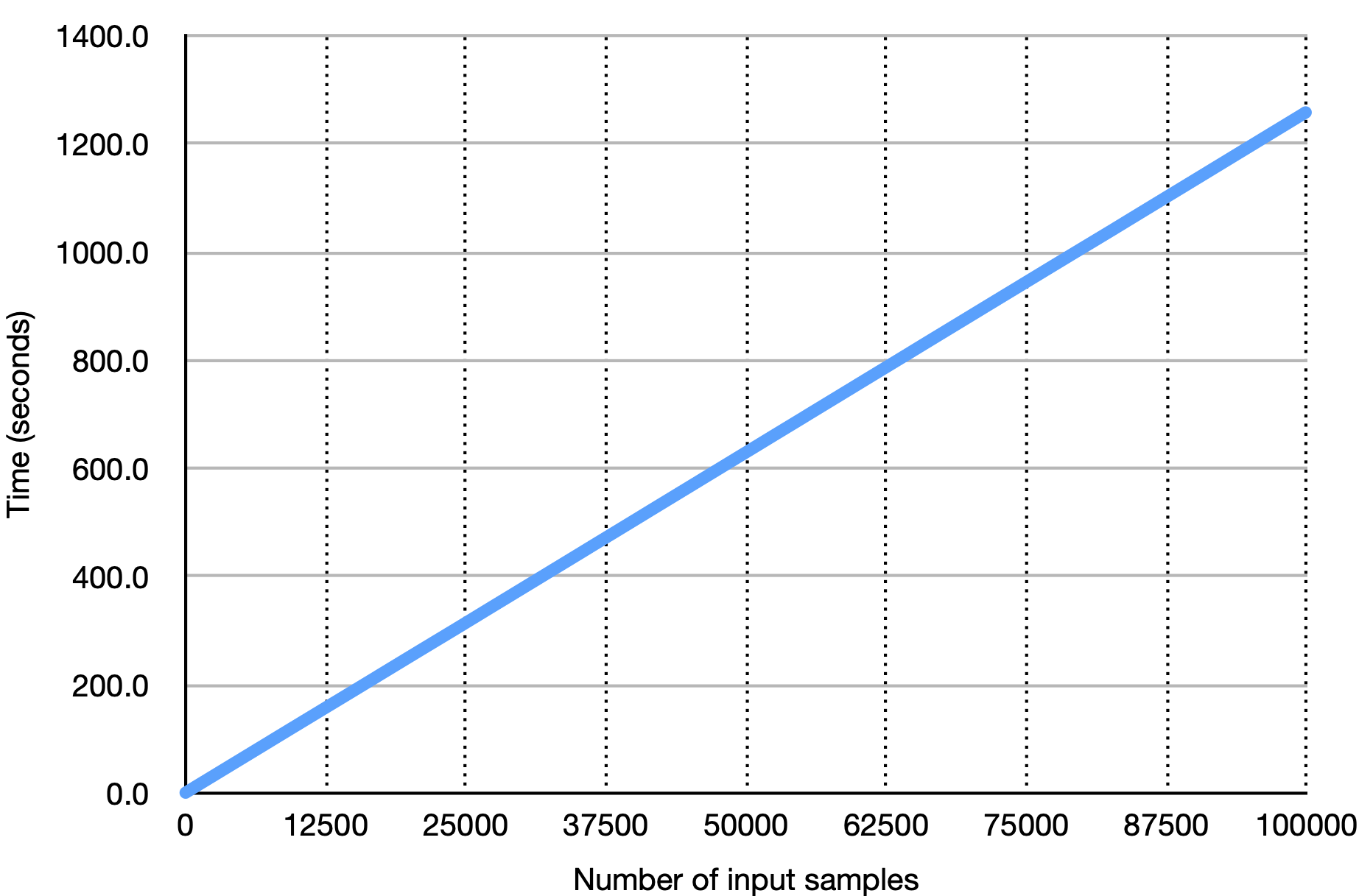
Figure 12: Runtime vs number of examples when extracting contextual embeddings using BERT

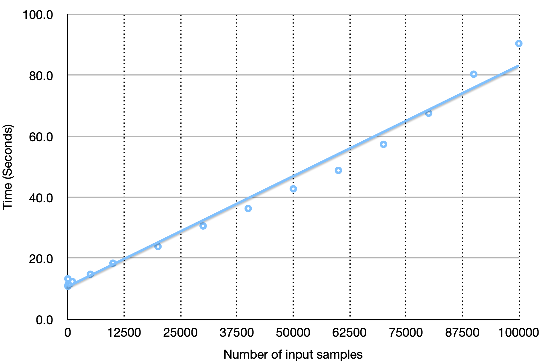
Figure 13: Runtime vs number of examples when performing correlation clustering

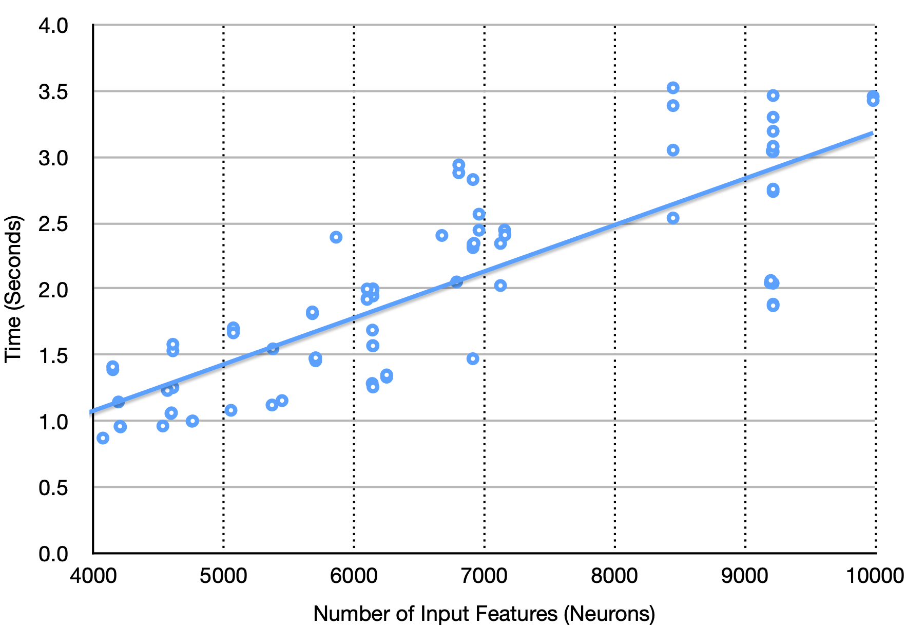
Figure 14: Runtime vs number of features when performing feature ranking using the weights of a trained classifier

A.6 Center Kernel Alignment

For layer-level redundancy, we compare representations from various layers using linear Center Kernel Alignment (cka - Kornblith et al. (2019)). Here, we briefly present the mathematical definitions behind cka. Let $\mathbf{Z}$ denote a column centering transformation. As denoted in the paper, ${\bm{z}}_{j}^{i}$ represents the contextualized embedding for some word $w_{j}$ at some layer $l_{i}$. Let ${\bm{z}}^{i}$ represent the contextual embeddings over all $T$ words, i.e. it is of size $T\times N$ (where $N$ is the total number of neurons). Given two layers $x$ and $y$,

$$\mathbf{X},\mathbf{Y}=\mathbf{Z}{\bm{z}}^{x},\mathbf{Z}{\bm{z}}^{y}$$

the CKA similarity is

$${\tt cka}({\bm{z}}^{x},{\bm{z}}^{y}):=\frac{\|\mathbf{X}^{T}\mathbf{Y}\|^{2}}{\|\mathbf{X}^{T}\mathbf{X}\|\|\mathbf{Y}^{T}\mathbf{Y}\|}$$

where $\|\cdot\|$ is the Frobenius norm.

References

- Abzianidze and Bos (2017) Lasha Abzianidze and Johan Bos. 2017. Towards universal semantic tagging. In Proceedings of the 12th International Conference on Computational Semantics (IWCS 2017) – Short Papers, pages 1–6, Montpellier, France.
- Andrew et al. (2013) Galen Andrew, Raman Arora, Jeff A. Bilmes, and Karen Livescu. 2013. Deep canonical correlation analysis. In Proceedings of the 30th International Conference on Machine Learning, ICML 2013, Atlanta, GA, USA, 16-21 June 2013, volume 28 of JMLR Workshop and Conference Proceedings, pages 1247–1255. JMLR.org.
- Bansal et al. (2004) Nikhil Bansal, Avrim Blum, and Shuchi Chawla. 2004. Correlation clustering. Machine Learning, 56(1–3):89–113.
- Bau et al. (2019) D. Anthony Bau, Yonatan Belinkov, Hassan Sajjad, Nadir Durrani, Fahim Dalvi, and James Glass. 2019. Identifying and controlling important neurons in neural machine translation. In International Conference on Learning Representations (ICLR).
- Belinkov et al. (2017) Yonatan Belinkov, Nadir Durrani, Fahim Dalvi, Hassan Sajjad, and James Glass. 2017. What do Neural Machine Translation Models Learn about Morphology? In Proceedings of the 55th Annual Meeting of the Association for Computational Linguistics (ACL), Vancouver. Association for Computational Linguistics.
- Belinkov et al. (2020) Yonatan Belinkov, Nadir Durrani, Fahim Dalvi, Hassan Sajjad, and James Glass. 2020. On the linguistic representational power of neural machine translation models. Computational Linguistics, 45(1):1–57.
- Bentivogli et al. (2009) Luisa Bentivogli, Ido Dagan, Hoa Trang Dang, Danilo Giampiccolo, and Bernardo Magnini. 2009. The fifth PASCAL recognizing textual entailment challenge. In Proceedings of the Second Text Analysis Conference, TAC 2009, Gaithersburg, Maryland, USA, November 16-17, 2009. NIST.
- Bouchacourt and Baroni (2018) Diane Bouchacourt and Marco Baroni. 2018. How agents see things: On visual representations in an emergent language game. In Proceedings of the 2018 Conference on Empirical Methods in Natural Language Processing, pages 981–985, Brussels, Belgium. Association for Computational Linguistics.
- Cao et al. (2020) Qingqing Cao, Harsh Trivedi, Aruna Balasubramanian, et al. 2020. Faster and just as accurate: A simple decomposition for transformer models. ICLR Openreview.
- Cer et al. (2017) Daniel Cer, Mona Diab, Eneko Agirre, Iñigo Lopez-Gazpio, and Lucia Specia. 2017. SemEval-2017 task 1: Semantic textual similarity multilingual and crosslingual focused evaluation. In Proceedings of the 11th International Workshop on Semantic Evaluation (SemEval-2017), pages 1–14, Vancouver, Canada. Association for Computational Linguistics.
- Chrupała (2019) Grzegorz Chrupała. 2019. Symbolic inductive bias for visually grounded learning of spoken language. In Proceedings of the 57th Annual Meeting of the Association for Computational Linguistics, pages 6452–6462, Florence, Italy. Association for Computational Linguistics.
- Chrupała and Alishahi (2019) Grzegorz Chrupała and Afra Alishahi. 2019. Correlating neural and symbolic representations of language. In Proceedings of the 57th Annual Meeting of the Association for Computational Linguistics, pages 2952–2962, Florence, Italy. Association for Computational Linguistics.
- Conneau et al. (2018) Alexis Conneau, German Kruszewski, Guillaume Lample, Loïc Barrault, and Marco Baroni. 2018. What you can cram into a single vector: Probing sentence embeddings for linguistic properties. In Proceedings of the 56th Annual Meeting of the Association for Computational Linguistics (ACL).
- Dalvi et al. (2019) Fahim Dalvi, Nadir Durrani, Hassan Sajjad, Yonatan Belinkov, D. Anthony Bau, and James Glass. 2019. What is one grain of sand in the desert? analyzing individual neurons in deep nlp models. In Proceedings of the Thirty-Third AAAI Conference on Artificial Intelligence (AAAI, Oral presentation).
- Devlin et al. (2019) Jacob Devlin, Ming-Wei Chang, Kenton Lee, and Kristina Toutanova. 2019. BERT: Pre-training of deep bidirectional transformers for language understanding. In Proceedings of the 2019 Conference of the North American Chapter of the Association for Computational Linguistics: Human Language Technologies, Volume 1 (Long and Short Papers), Minneapolis, Minnesota. Association for Computational Linguistics.
- Dolan and Brockett (2005) William B. Dolan and Chris Brockett. 2005. Automatically constructing a corpus of sentential paraphrases. In Proceedings of the Third International Workshop on Paraphrasing (IWP2005).
- Durrani et al. (2019) Nadir Durrani, Fahim Dalvi, Hassan Sajjad, Yonatan Belinkov, and Preslav Nakov. 2019. One size does not fit all: Comparing NMT representations of different granularities. In Proceedings of the 2019 Conference of the North American Chapter of the Association for Computational Linguistics: Human Language Technologies, Volume 1 (Long and Short Papers), pages 1504–1516, Minneapolis, Minnesota. Association for Computational Linguistics.
- Durrani et al. (2020) Nadir Durrani, Hassan Sajjad, Fahim Dalvi, and Yonatan Belinkov. 2020. Analyzing individual neurons in pretrained language models. In Proceedings of the 2020 Conference on Empirical Methods in Natural Language Processing (EMNLP-2020), Online. Association for Computational Linguistics.
- Ethayarajh (2019) Kawin Ethayarajh. 2019. How contextual are contextualized word representations? comparing the geometry of BERT, ELMo, and GPT-2 embeddings. In Proceedings of the 2019 Conference on Empirical Methods in Natural Language Processing and the 9th International Joint Conference on Natural Language Processing (EMNLP-IJCNLP), pages 55–65, Hong Kong, China. Association for Computational Linguistics.
- Fan et al. (2020) Angela Fan, Edouard Grave, and Armand Joulin. 2020. Reducing transformer depth on demand with structured dropout. In 8th International Conference on Learning Representations, ICLR 2020, Addis Ababa, Ethiopia, April 26-30, 2020. OpenReview.net.
- Gordon et al. (2020) Mitchell A. Gordon, Kevin Duh, and Nicholas Andrews. 2020. Compressing BERT: studying the effects of weight pruning on transfer learning. In Proceedings of the 5th Workshop on Representation Learning for NLP, RepL4NLP@ACL 2020, Online, July 9, 2020, pages 143–155. Association for Computational Linguistics.
- Guyon and Elisseeff (2003) Isabelle Guyon and André Elisseeff. 2003. An introduction to variable and feature selection. Journal of Machine Learning Research, 3:1157–1182.
- Hameed (2018) Shilan Hameed. 2018. Filter-wrapper combination and embedded feature selection for gene expression data. International Journal of Advances in Soft Computing and its Applications, 10:90–105.
- Hao et al. (2019) Yaru Hao, Li Dong, Furu Wei, and Ke Xu. 2019. Visualizing and understanding the effectiveness of BERT. In Proceedings of the 2019 Conference on Empirical Methods in Natural Language Processing and the 9th International Joint Conference on Natural Language Processing (EMNLP-IJCNLP), pages 4141–4150, Hong Kong, China. Association for Computational Linguistics.
- Hewitt and Liang (2019) John Hewitt and Percy Liang. 2019. Designing and interpreting probes with control tasks. In Proceedings of the 2019 Conference on Empirical Methods in Natural Language Processing and the 9th International Joint Conference on Natural Language Processing (EMNLP-IJCNLP), pages 2733–2743, Hong Kong, China. Association for Computational Linguistics.
- Hockenmaier (2006) Julia Hockenmaier. 2006. Creating a CCGbank and a wide-coverage CCG lexicon for German. In Proceedings of the 21st International Conference on Computational Linguistics and 44th Annual Meeting of the Association for Computational Linguistics, ACL ’06, pages 505–512, Sydney, Australia.
- Hupkes et al. (2018) Dieuwke Hupkes, Sara Veldhoen, and Willem Zuidema. 2018. Visualisation and ‘diagnostic classifiers’ reveal how recurrent and recursive neural networks process hierarchical structure. Journal of Artificial Intelligence Research, 61:907–926.
- Kim et al. (2020) Taeuk Kim, Jihun Choi, Daniel Edmiston, and Sang-goo Lee. 2020. Are pre-trained language models aware of phrases? simple but strong baselines for grammar induction. In 8th International Conference on Learning Representations, ICLR 2020, Addis Ababa, Ethiopia, April 26-30, 2020. OpenReview.net.
- Kornblith et al. (2019) Simon Kornblith, Mohammad Norouzi, Honglak Lee, and Geoffrey Hinton. 2019. Similarity of neural network representations revisited. In Proceedings of the 36th International Conference on Machine Learning, volume 97 of Proceedings of Machine Learning Research, pages 3519–3529, Long Beach, California, USA. PMLR.
- Kriegeskorte et al. (2008) Nikolaus Kriegeskorte, Marieke Mur, and Peter Bandettini. 2008. Representational similarity analysis - connecting the branches of systems neuroscience. Frontiers in Systems Neuroscience, 2:4.
- Liu et al. (2019) Nelson F. Liu, Matt Gardner, Yonatan Belinkov, Matthew E. Peters, and Noah A. Smith. 2019. Linguistic knowledge and transferability of contextual representations. In Proceedings of the 2019 Conference of the North American Chapter of the Association for Computational Linguistics: Human Language Technologies, Volume 1 (Long and Short Papers), pages 1073–1094, Minneapolis, Minnesota. Association for Computational Linguistics.
- Marcus et al. (1993) Mitchell P. Marcus, Beatrice Santorini, and Mary Ann Marcinkiewicz. 1993. Building a large annotated corpus of English: The Penn Treebank. Computational Linguistics, 19(2):313–330.
- Michel et al. (2019) Paul Michel, Omer Levy, and Graham Neubig. 2019. Are sixteen heads really better than one? In H. Wallach, H. Larochelle, A. Beygelzimer, F. d'Alché-Buc, E. Fox, and R. Garnett, editors, Advances in Neural Information Processing Systems 32, pages 14014–14024. Curran Associates, Inc.
- Mu et al. (2018) Jiaqi Mu, Suma Bhat, and Pramod Viswanath. 2018. All-but-the-top: Simple and effective postprocessing for word representations. In 6th International Conference on Learning Representations, ICLR 2018, Vancouver, BC, Canada, April 30 - May 3, 2018, Conference Track Proceedings. OpenReview.net.
- Pimentel et al. (2020) Tiago Pimentel, Josef Valvoda, Rowan Hall Maudslay, Ran Zmigrod, Adina Williams, and Ryan Cotterell. 2020. Information-theoretic probing for linguistic structure. In Proceedings of the 58th Annual Meeting of the Association for Computational Linguistics, ACL 2020, Online, July 5-10, 2020, pages 4609–4622. Association for Computational Linguistics.
- Qian et al. (2016) Peng Qian, Xipeng Qiu, and Xuanjing Huang. 2016. Analyzing Linguistic Knowledge in Sequential Model of Sentence. In Proceedings of the 2016 Conference on Empirical Methods in Natural Language Processing, pages 826–835, Austin, Texas. Association for Computational Linguistics.
- Raffel et al. (2019) Colin Raffel, Noam Shazeer, Adam Roberts, Katherine Lee, Sharan Narang, Michael Matena, Yanqi Zhou, Wei Li, and Peter J. Liu. 2019. Exploring the limits of transfer learning with a unified text-to-text transformer. arXiv e-prints.
- Raghu et al. (2017) Maithra Raghu, Justin Gilmer, Jason Yosinski, and Jascha Sohl-Dickstein. 2017. SVCCA: Singular Vector Canonical Correlation Analysis for Deep Learning Dynamics and Interpretability. In I. Guyon, U. V. Luxburg, S. Bengio, H. Wallach, R. Fergus, S. Vishwanathan, and R. Garnett, editors, Advances in Neural Information Processing Systems 30, pages 6078–6087. Curran Associates, Inc.
- Rajpurkar et al. (2016) Pranav Rajpurkar, Jian Zhang, Konstantin Lopyrev, and Percy Liang. 2016. SQuAD: 100,000+ questions for machine comprehension of text. In Proceedings of the 2016 Conference on Empirical Methods in Natural Language Processing, pages 2383–2392, Austin, Texas. Association for Computational Linguistics.
- Sajjad et al. (2020) Hassan Sajjad, Fahim Dalvi, Nadir Durrani, and Preslav Nakov. 2020. Poor man’s bert: Smaller and faster transformer models. ArXiv, abs/2004.03844.
- Sang and Buchholz (2000) Erik F. Tjong Kim Sang and Sabine Buchholz. 2000. Introduction to the CoNLL-2000 shared task chunking. In Fourth Conference on Computational Natural Language Learning, CoNLL 2000, and the Second Learning Language in Logic Workshop, LLL 2000, Held in cooperation with ICGI-2000, Lisbon, Portugal, September 13-14, 2000, pages 127–132. ACL.
- Sanh et al. (2019) Victor Sanh, Lysandre Debut, Julien Chaumond, and Thomas Wolf. 2019. Distilbert, a distilled version of bert: smaller, faster, cheaper and lighter.
- Shen et al. (2020) Sheng Shen, Zhen Dong, Jiayu Ye, Linjian Ma, Zhewei Yao, Amir Gholami, Michael W. Mahoney, and Kurt Keutzer. 2020. Q-BERT: hessian based ultra low precision quantization of BERT. In The Thirty-Fourth AAAI Conference on Artificial Intelligence, AAAI 2020, The Thirty-Second Innovative Applications of Artificial Intelligence Conference, IAAI 2020, The Tenth AAAI Symposium on Educational Advances in Artificial Intelligence, EAAI 2020, New York, NY, USA, February 7-12, 2020, pages 8815–8821. AAAI Press.
- Shi et al. (2016a) Xing Shi, Kevin Knight, and Deniz Yuret. 2016a. Why neural translations are the right length. In Proceedings of the 2016 Conference on Empirical Methods in Natural Language Processing, pages 2278–2282, Austin, Texas. Association for Computational Linguistics.
- Shi et al. (2016b) Xing Shi, Inkit Padhi, and Kevin Knight. 2016b. Does string-based neural MT learn source syntax? In Proceedings of the 2016 Conference on Empirical Methods in Natural Language Processing, EMNLP 2016, Austin, Texas, USA, November 1-4, 2016, pages 1526–1534. The Association for Computational Linguistics.
- Socher et al. (2013) Richard Socher, Alex Perelygin, Jean Wu, Jason Chuang, Christopher D. Manning, Andrew Ng, and Christopher Potts. 2013. Recursive deep models for semantic compositionality over a sentiment treebank. In Proceedings of the 2013 Conference on Empirical Methods in Natural Language Processing, pages 1631–1642, Seattle, Washington, USA. Association for Computational Linguistics.
- Suau et al. (2020) Xavier Suau, Luca Zappella, and Nicholas Apostoloff. 2020. Finding experts in transformer models. CoRR, abs/2005.07647.
- Sun et al. (2019) Siqi Sun, Yu Cheng, Zhe Gan, and Jingjing Liu. 2019. Patient knowledge distillation for BERT model compression. In Proceedings of the 2019 Conference on Empirical Methods in Natural Language Processing and the 9th International Joint Conference on Natural Language Processing (EMNLP-IJCNLP), pages 4322–4331, Hong Kong, China. Association for Computational Linguistics.
- Tenney et al. (2019) Ian Tenney, Patrick Xia, Berlin Chen, Alex Wang, Adam Poliak, R. Thomas McCoy, Najoung Kim, Benjamin Van Durme, Samuel R. Bowman, Dipanjan Das, and Ellie Pavlick. 2019. What do you learn from context? probing for sentence structure in contextualized word representations. In 7th International Conference on Learning Representations, ICLR 2019, New Orleans, LA, USA, May 6-9, 2019. OpenReview.net.
- Turc et al. (2019) Iulia Turc, Ming-Wei Chang, Kenton Lee, and Kristina Toutanova. 2019. Well-read students learn better: The impact of student initialization on knowledge distillation. CoRR, abs/1908.08962.
- Voita et al. (2019) Elena Voita, David Talbot, Fedor Moiseev, Rico Sennrich, and Ivan Titov. 2019. Analyzing multi-head self-attention: Specialized heads do the heavy lifting, the rest can be pruned. In Proceedings of the 57th Annual Meeting of the Association for Computational Linguistics, pages 5797–5808, Florence, Italy. Association for Computational Linguistics.
- Voita and Titov (2020) Elena Voita and Ivan Titov. 2020. Information-theoretic probing with minimum description length. In Proceedings of the 2020 Conference on Empirical Methods in Natural Language Processing. Association for Computational Linguistics.
- Wang et al. (2018) Alex Wang, Amanpreet Singh, Julian Michael, Felix Hill, Omer Levy, and Samuel Bowman. 2018. GLUE: A multi-task benchmark and analysis platform for natural language understanding. In Proceedings of the 2018 EMNLP Workshop BlackboxNLP: Analyzing and Interpreting Neural Networks for NLP, pages 353–355, Brussels, Belgium. Association for Computational Linguistics.
- Williams et al. (2018) Adina Williams, Nikita Nangia, and Samuel Bowman. 2018. A broad-coverage challenge corpus for sentence understanding through inference. In Proceedings of the 2018 Conference of the North American Chapter of the Association for Computational Linguistics: Human Language Technologies, Volume 1 (Long Papers), pages 1112–1122, New Orleans, Louisiana. Association for Computational Linguistics.
- Wolf et al. (2019) Thomas Wolf, Lysandre Debut, Victor Sanh, Julien Chaumond, Clement Delangue, Anthony Moi, Pierric Cistac, Tim Rault, Rémi Louf, Morgan Funtowicz, Joe Davison, Sam Shleifer, Patrick von Platen, Clara Ma, Yacine Jernite, Julien Plu, Canwen Xu, Teven Le Scao, Sylvain Gugger, Mariama Drame, Quentin Lhoest, and Alexander M. Rush. 2019. Huggingface’s transformers: State-of-the-art natural language processing. ArXiv, abs/1910.03771.
- Wu et al. (2020) John M. Wu, Yonatan Belinkov, Hassan Sajjad, Nadir Durrani, Fahim Dalvi, and James R. Glass. 2020. Similarity analysis of contextual word representation models. In Proceedings of the 58th Annual Meeting of the Association for Computational Linguistics, ACL 2020, Online, July 5-10, 2020, pages 4638–4655. Association for Computational Linguistics.
- Yang et al. (2019) Zhilin Yang, Zihang Dai, Yiming Yang, Jaime G. Carbonell, Ruslan Salakhutdinov, and Quoc V. Le. 2019. XLNet: Generalized autoregressive pretraining for language understanding. In Advances in Neural Information Processing Systems 32: Annual Conference on Neural Information Processing Systems 2019, NeurIPS 2019, 8-14 December 2019, Vancouver, BC, Canada, pages 5754–5764.