New molecular species at redshift $z=0.89$

We present the first detections of CH₃SH, C₃H⁺, C₃N, HCOOH, CH₂CHCN, and H₂CN in an extragalactic source. Namely the spiral arm of a galaxy located at $z=0.89$ on the line of sight to the radio-loud quasar PKS 1830$-$211. OCS, SO₂, and NH₂CN were also detected, raising the total number of molecular species identified in that early time galaxy to 54, not counting isotopologues. The detections were made in absorption against the SW quasar image, at 2 kpc from the galaxy centre, over the course of a Q band spectral line survey made with the Yebes 40 m telescope (rest-frame frequencies: 58.7 $-$ 93.5 GHz). We derived the rotational temperatures and column densities of those species, which are found to be subthermally excited. The molecular abundances, and in particular the large abundances of C₃H⁺ and of several previously reported cations, are characteristic of diffuse or translucent clouds with enhanced UV radiation or strong shocks.

1 Introduction

Some 220 molecular species, not counting isotopologues, have been identified in the galactic interstellar medium (ISM). Among them are ions, neutral radicals, metallic compounds, and complex organic molecules (COMs), whose relative abundances and isotopic ratios vary drastically due to the type of source and environment (see CDMS). Conversely, the observation of molecular abundances offers a powerful way to characterise the gas properties and past history. This is particularly true for distant galaxies where we lack spatial resolution.

Distant galaxies tell us about the earlier stages of the ISM. Heavy elements and metals appeared early on in the ISM after a first generation of massive stars released their nucleosynthesis products into space. Secondary elements, such as nitrogen, mostly appeared several billions of years later; after a second generation of stars, low-mass longer-lived stars released their processed material (Johnson 2019). The chemical and isotopic composition of the ISM in a galaxy at redshift $z=1$, when the Universe was half its present age, should therefore be markedly different from that in the Galaxy and be dominated by the products of massive stars (Muller et al. 2011). An analysis of the molecular content and isotopic ratios in distant galaxies, thus, offers us an opportunity to characterise these types of sources and to check current models of galaxy chemical evolution.

A powerful method to study the ISM of distant galaxies is through the detection of molecular lines in absorption. The strength of the absorption depends on the flux of the background source and the line opacity. The latter can be directly obtained and, if the background quasar image is small enough to be fully covered by the absorbing gas, this strength is decoupled from the distance to the absorber. Therefore, it is not diluted by the telescope beam, allowing for the detection of low abundance species in distant sources.

One of the most studied molecular absorbers is the system located towards the blazar PKS 1830$-$211 at redshift $z=2.5$ (Lidman et al. 1999; see Muller et al. 2006 for a detailed description of the system). The blazar image is gravitationally lensed by a foreground, nearly face-on spiral galaxy at $z=0.89$ that intercepts the line of sight (Wiklind & Combes 1996; Winn et al. 2002). At radio wavelengths, lensing gives rise to two point-like images of the blazar, embedded in a faint Einstein ring of 1^′′ in diameter (8 kpc at the distance of the galaxy, Jauncey et al. 1991). The two bright images, that is, only the ones that are still present at millimetre wavelengths, are located 2 kpc SW and 6 kpc NE of the galaxy nucleus, respectively. The redshift of $z$ = 0.89 corresponds to an age of 6.4 Gyr (see Wright 2006 for the assumed cosmological parameters) and hence to a lookback time close to half the present age of the Universe.

The molecular absorption arises in two spiral arms symmetrically unrolling on either side of the nucleus (Wiklind & Combes 1996). Several studies using millimetre interferometers (NOEMA, ATCA, and ALMA) have revealed the molecular richness of the SW arm (Muller et al. 2006, 2011, 2013, 2014b, 2014a, 2016a, 2016b, 2017; Müller et al. 2015). More than 45 molecular species, plus more than 15 rare isotopologues, have been reported in those studies. Among others, they consist of COMs (such as CH₃OH, CH₃CN, NH₂CHO, and CH₃CHO), of hydrocarbons (l-C₃H, l-C₃H₂, and C₄H), and of light hydrides and cations (H₂Cl⁺, ArH⁺, CF⁺, OH⁺, H₂O⁺, CH⁺, and SH⁺). Muller et al. (2011, 2014b) suggest that this denotes a chemical signature similar to that of the galactic diffuse and translucent clouds. Furthermore, the analysis of the light hydrides detected in this source points out a multi-phase composition of the absorbing gas (Muller et al. 2016a, b).

PKS 1830$-$211 is also a strong gamma-ray emitter, with several flaring events in recent years (see e.g. Abdo et al. 2015). During 2019, flares of intense gamma-ray activity were reported using the Large Area Telescope (LAT), one of the two instruments on board the Fermi Gamma-ray Space Telescope (Buson & Constantin 2019). The preliminary analysis conducted by the Fermi-LAT collaboration indicates that this source has been undergoing a long-term brightening since October 2018. Following this gamma-ray outburst, a radio-wave monitoring campaign with the 32 m Medicina and 64 m Sardinia radio telescopes, at 8.3 GHz and 25.4 GHz, has revealed a parallel radio emission enhancement (Iacolina et al. 2019).

We took advantage of this event to search for new extragalactic molecular species with the Yebes 40 m radio telescope, whose 7 mm receiver was recently updated with the help of the European Research Council NANOCOSMOS project. In this Letter, we report the detection of six new extragalactic molecular species towards the SW image of PKS 1830$-$211. We derived their molecular column densities and rotational temperatures, as well as those of three more species that were detected for the first time in this source (Section 4). In light of the new identifications, we discuss the implications for the prevailing chemistry in the source (Section 5).

2 Observations and data reduction

The observations began in April 2019 with the 40 m diameter Yebes radio telescope, just after the recent enhancement of the blazar radio flux (Buson & Constantin 2019; Iacolina et al. 2019). They consisted in monitoring the continuum flux and absorption line profiles in the course of commissioning the new 7 mm receiver (F. Tercero et al. in preparation). The telescope (de Vicente et al. 2016) is located at 990 m of altitude near Guadalajara, Spain.

The Q band (7 mm) HEMT receiver allows for simultaneous broad-band observations in two linear polarisations. It is connected to 16 fast Fourier transform spectrometers (FFTS), each covering 2.5 GHz with a 38 kHz channel separation. In each polarisation, this system provides an instantaneous band of 18 GHz between 31.5 GHz and 50 GHz.

The 7 mm spectra shown in this paper are the average of 12 observing sessions, which were carried out between April 2019 and September 2019. Due to the low declination of the source, it could only be observed for 5 hours per day above 15^∘ elevation (the telescope latitude is $+$40^∘ 31^′ 29.6^′′). The intensity scale was calibrated using two absorbers at different temperatures and the atmospheric transmission model (ATM, Cernicharo 1985; Pardo et al. 2001).

In addition, we carried out three observing sessions at 1.3 cm with the K band receiver on May 29 and 30 as well as June 2. The goal of those observations was to confirm the identification of C₃H⁺ by observing a third rotational transition. The covered band extended from 23.7 GHz to 24.2 GHz, and the channel spacing was 30 kHz. For these data, the intensity scale was calibrated using a noise diode and the ATM model.

The observational procedure was position switching with the reference position located $-$240^′′ away in azimuth. The telescope pointing and focus were checked every one to two hours through pseudo-continuum observations of VX Sgr, a red hypergiant star close to the target source. VX Sgr shows strong SiO $v$ = 1 $J$ = 1$-$0 (at 43.122 GHz) and H₂O $J_{K_{a},K_{c}}$ = 6_1,6$-$5_2,3 (at 22.235 GHz) maser emission. Pseudo-continuum observations consist in subtracting the summed spectral emission from the masers from the rest of the spectrum, while performing pointing azimuth-elevation cross drifts or a focus scan. This is a useful technique since atmospheric emissivity fluctuations during the scans have a small influence on the results and provide very flat continuum baselines. In addition, we regularly checked the pointing towards the blazar PKS 1830$-$211 itself (coordinates $\upalpha_{\rm J2000}$ = 18^h 33^m 39.9^s, $\updelta_{\rm J2000}$ = $-$21^∘ 03^′ 39.6^′′), whose flux (NE + SW images) was $\simeq$ 10 Jy at intermediate frequencies of the 7 mm band. The pointing errors were always found $<5^{\prime\prime}$ on both axes. In order to confirm that no spurious signals were contaminating our spectra, the frequency of the local oscillator was changed by 20 MHz from one observing session to the next.

The data were reduced using the CLASS software of the GILDAS package. A polynomial baseline of low order (typically second or third order) was removed from the spectrum obtained for each session. All sessions were then averaged together. In this paper, we adopt $z$ = 0.885875 ($v_{0}$ = 0 km s^-1 in the local standard of rest, LSR) to convert the observed frequencies to rest-frame frequencies. For each observed frequency, Table 2 lists the telescope aperture efficiency ($\eta_{\rm A}$), the conversion factor between flux ($S$) and antenna temperature ($T_{\rm A}^{*}$), the half power beam width (HPBW), the system temperature ($T_{\rm sys}$), the integration time, and the noise root mean square (rms).

3 Continuum emission

The intensity scales of the spectra shown in this Letter were normalised to the total (NE + SW) continuum intensity of the source. The latter varies with frequency as indicated (in $T_{A}^{*}$ scale) in Table 2. The molecular lines presented in this article all appear in absorption against the SW image (the NE image absorption, which is much weaker, appears at markedly different velocities). In order to derive the line opacities, we had to determine the contribution of the SW image to the total continuum flux detected by the telescope. This can be done by assuming that the HCO⁺ and HCN ($J=1-0$) line absorption (see Fig. 2) is at its total at velocities near $v_{0}=0$ km s^-1, which corresponds to the arm located in front of the SW source. This assumption, which was already discussed by Muller & Guélin (2008) for the $J=2-1$ lines, is supported by the obvious saturation of the flattened absorption profiles and by the near-stability of the saturation level despite strong blazar intensity variations.

Muller & Guélin (2008) measured a roughly constant flux ratio of the NE to SW components, $R$ $\sim$ 1.7, over several observations between 1995 and 2007 at 3 mm. This value is similar to that obtained by Subrahmanyan et al. (1990) at the centimetre wavelengths. Using ATCA data from 2011, Muller et al. (2013) derived an $R$ of $\sim$1.5 at 3 mm and 7 mm. Following the strategy of Muller & Guélin (2008), we estimated the NE/SW flux ratio using the $J=1-0$ HCO⁺ and HCN lines. As these saturated lines absorb 45 % of the total flux, the NE component (with the residual emission of the faint Einstein ring) has to contribute 55 % to the total flux. We obtain a rather constant value of $R$ $\sim$ 1.2 over the period from April to September 2019 (see Fig. 2). This value is close to that measured by Muller et al. (2014b) at 250 GHz and 290 GHz from ALMA data from April 9 and 11, 2012, respectively, just before a gamma-ray flare. It is, however, significantly lower than in most of the other measurements at millimetre and submillimetre wavelengths (see also Marti-Vidal & Muller 2019). This is perhaps due to a conjunction between the blazar flux variations and the four-week delay between the NE and SW light paths. These flux variations are thought to be associated with plasmon ejections along the precessing jet of the blazar (Nair et al. 2005; Muller & Guélin 2008).

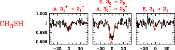
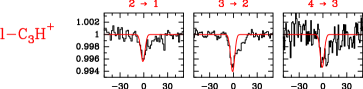
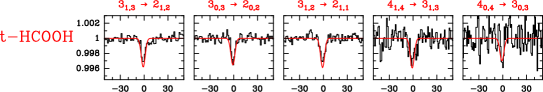
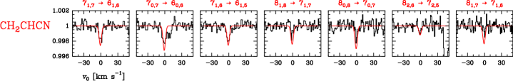
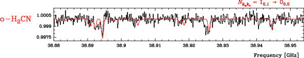
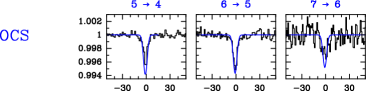
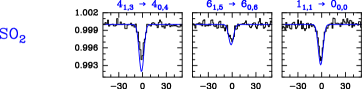
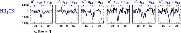
Figure 1: Absorption lines towards PKS 1830$-$211 observed with the Yebes 40 m telescope. The species identified for the first time in an extragalactic source are highlighted in red. The molecules highlighted in blue are those that were identified for the first time in this source, but observed previously in other extragalactic sources. The $y$-axis is the normalised intensity to the total (NE + SW) continuum level (see Sect. 3). We assume a $z$ = 0.885875 ($v_{\rm 0}$ = 0 km s^-1 in the local standard of rest).

4 Results

Table 1: Dipole moments ($\mu$), number of detected lines, table number listing the spectroscopic and observational line parameters, rotational temperatures ($T_{\rm rot}$) and column densities ($N$) obtained with the rotational diagram (RD) analysis, and physical parameters assumed for the MADEX LTE model of the new molecules detected in this work.

				RD analysis			MADEX LTE model
Molecule	$\mu$	No. Lines	Table	$T_{\rm rot}$	$N$ $\times$ 1012		$v_{\rm 0}$	$v_{\rm FWHM}$	$T_{\rm rot}$	$N$ $\times$ 1012	Notes
	[Debye]			[K]	[cm-2]		[km s-1]	[km s-1]	[K]	[cm-2]
A/E-CH3SH	$\mu_{a}$=1.3a	3	3	…	…		$-$1.0	7.0	5.0	20
l-C3H+	$\mu_{a}$=3.0b	3	4	5 $\pm$ 1	1.2 $\pm$ 0.2		$-$0.6	6.0	5.0	1.0
C3N	$\mu_{a}$=2.8c	4	5	5 $\pm$ 1	4 $\pm$ 1		$-$0.5	5.0	5.0	3.0	$\dagger$
t-HCOOH	$\mu_{a}$=1.4d	5	6	5 $\pm$ 1	2.3 $\pm$ 0.5		$-$0.7	6.0	5.0	2.3	*
				6 $\pm$ 1	3.3 $\pm$ 0.4		$-$0.7	6.0	6.0	3.3	**
					6 $\pm$ 2						***
CH2CHCN	$\mu_{a}$=3.8e	7	7	10 $\pm$ 4	5 $\pm$ 2		$-$0.5	5.0	10	5.5
o-H2CN	$\mu_{a}$=2.5f	4	8	…	…		$-$1.0	5.0	5.0	4.0
OCS	$\mu_{a}$=0.7g	3	9	8 $\pm$ 3	43 $\pm$ 15		$-$0.7	5.5	8.0	43
SO2	$\mu_{b}$=1.6h	3	10	8 $\pm$ 1	25 $\pm$ 4		$-$0.9	7.0	8.0	25
O+-NH2CN	$\mu_{a}$=4.3i	6	11	30 $\pm$ 5	11 $\pm$ 2		$-$0.9	7.0	30	11

For the first time, we detected CH₃SH, C₃H⁺, C₃N, HCOOH, CH₂CHCN, and H₂CN in an extragalactic source and identified the following three more species, also for the first time, towards PKS 1830$-$211: OCS, SO₂, and NH₂CN. All of those species have been detected in absorption towards the SW spiral arm of the $z$ = 0.89 galaxy in front of the blazar. Figure 1 shows these detections. For each species, Table 1 lists its dipole moment and derived properties.

A single Gaussian profile was fitted to the strongest component of all detected lines to obtain the observational line parameters: radial velocities ($v_{\rm 0}$), full width at half maximum (FWHM) line widths ($v_{\rm FWHM}$), and absorption intensities ($I_{\rm\nu}$) measured from the unity on the normalised spectrum to the total (SW + NW) continuum level (see Sect. 3). Then, optical depths ($\tau_{\rm\nu}$) towards the SW line of sight were directly derived according to

$$\tau_{\rm\nu}=-{\rm ln}\left(1-\frac{I_{\rm\nu}}{0.45}\right),$$ (1)

assuming an SW source covering factor of unity (see e.g. Muller & Guélin 2008 and Muller et al. 2011; these references also address a more general discussion regarding how to obtain optical depths of absorbing lines in this source). This assumption does not introduce major uncertainties since Muller et al. (2014b), using ALMA observations, conclude that the size of the SW continuum image is only 5 $-$ 10 % larger than the size of the absorbing gas at millimetre and submillimetre wavelengths. These results, together with the spectroscopic parameters of the involved transitions are shown in Tables 3 $-$ 11. We note that while the derived radial velocities are in agreement with previous observations at 7 mm towards the SW line of sight (Muller et al. 2011, 2013), most of the line widths of the molecular lines in our data are in a range between 5 $-$10 km s^-1. Our absorbing molecular lines are narrower than those of these previous works by a factor of 2. Narrower lines may indicate either lower optical depths or different clouds intercepting the line of sight. This variation could result from the appearance or disappearance of discrete components in the background continuum source (Muller & Guélin 2008).

As we detected several rotational transitions for many species, we estimated their rotational temperatures ($T_{\rm rot}$) and molecular column densities ($N$) by drawing rotational diagrams. The analysis assumes the Rayleigh-Jeans approximation, optically thin lines, and local thermodynamic equilibrium (LTE). In Appendix C, we describe this method and the diagrams relative to this work (Fig. 3). The resulting $T_{\rm rot}$ and $N$ are given in Table 1.

We note that the $T_{\rm rot}$ obtained for C₃H⁺, C₃N, and HCOOH is close to the temperature of the cosmic microwave background (CMB) at $z$ = 0.89 ($T_{\rm CMB}$ = 5.08 $\pm$ 0.10 K, Muller et al. 2013). This result was already noted in previous surveys (Combes & Wiklind 1999; Menten et al. 1999; Henkel et al. 2009; Muller et al. 2011, 2013). It implies an excitation dominated by radiative coupling with the CMB since the gas kinetic temperature in the SW source is found from NH₃ lines that are much higher ($\sim$80 K, according to Henkel et al. 2008). It also means that the bulk of the gas has a moderate or low density: $\leq 10^{3}$ cm^-3 (e.g. Henkel et al. 2009; Muller et al. 2013).

It is important to note that CH₂CHCN, OCS, and SO₂ have a somewhat higher $T_{\rm rot}$ (8 $-$ 10 K). This suggests that either the observed lines arise in the denser parts of the absorbing clouds or these molecules present lower critical densities than those of C₃H⁺, C₃N, and HCOOH, which are, therefore, more sensitive to collisions.

The case is more extreme for NH₂CN for which we find $T_{\rm rot}=30$ K. Interestingly enough, the lines pertaining to the two different $K_{\rm a}$ ladders of that latter species merge into a single straight line in the rotational diagram after correcting for the different statistical weights. This is typical of asymmetric top molecules in dense environments (see Appendix C). As we mention above, these results may indicate that either NH₂CN traces a denser and hotter component of the absorbing gas or a surprisingly low critical density for this species.

To confirm the line identifications, we produced synthetic spectra of the putative species using the MADEX tool (Cernicharo 2012). For this, we assumed LTE approximation and adopted the $T_{\rm rot}$ and $N$ values derived from the rotational diagrams. In the cases of CH₃SH and H₂CN, for which we do not have enough lines to draw a rotational diagram, we fixed $T_{\rm rot}$ to 5 K and varied $N$ until we obtained a reasonable fit to the line profiles. The $T_{\rm rot}$ and $N$ values as well as the fitted $v_{\rm 0}$ and $v_{\rm FWHM}$ for all species are shown in Table 1. Since MADEX computes the line opacities in the absence of a continuum background source ($\tau_{\rm\nu}$), we derived the line absorption profile against the SW continuum image, normalised to the total (NE + SW) continuum emission by re-arranging Eq. 1 to obtain $I_{\rm\nu}$. We note that the absorption by the SW spiral arm occurs at velocities of $0\pm 50$ km s^-1, which are quite different from those caused by the NE arm around $-$140 km s^-1, and that no absorption is detected at the latter velocity for the nine species considered here. The resulting synthetic spectrum is overlaid over the observed lines in Fig. 1. This simple model reproduces the observed lines. The model also allows us to distinguish an additional component for C₃H⁺ and H₂CN between 0 km s^-1 and 10 km s^-1 that was not taken into account in our model. This component is also seen in the lowest energy lines of CH₃SH and CH₂CHCN. However, the weakness of this component in the mentioned lines prevents us from further evaluating its properties.

5 Discussion

This work expands the inventory of extragalactic species, particularly in the SW line of sight towards PKS 1830$-$211 with the detection of nine new species. With these new species, the number of molecular species towards the SW line of sight of PKS 1830$-$211 raises to more than 50.

The sample of molecules detected here points to a large diversity in molecular environments:

1. Carbon chains (C₃N) and ion-molecule gas phase-produced $-$CN species (H₂CN and CH₂CHCN) have been detected in dense ($\sim$10⁴ cm^-3) and cold ($T_{\rm K}$ $\sim$ 10 K) prestellar cores (Ohishi et al. 1994; Kaifu et al. 2004) of our Galaxy.

2. CH₃SH and NH₂CN have only been detected towards hot cores in high-mass star-forming regions (Turner et al. 1975; Linke et al. 1979; Kolesniková et al. 2014) and low-mass protostars (Cernicharo et al. 2012; Majumdar et al. 2016; Coutens et al. 2018). NH₂CN has also been detected in the starburst galaxies M32 and NGC253 (Martín et al. 2006; Aladro et al. 2011). Besides prestellar cores, CH₂CHCN is an abundant species in hot cores (Belloche et al. 2013; López et al. 2014).

3. Although OCS, SO₂, and HCOOH have been detected in a large variety of environments, these molecules usually trace hot and shocked gas in star forming regions (Tercero et al. 2010; Esplugues et al. 2013; Tercero et al. 2018) .

4. C₃H⁺ traces the edge of dense molecular clouds illuminated by UV radiation. In our Galaxy, this species has only been unambiguously detected towards the Horsehead and the Orion Bar (Pety et al. 2012; McGuire et al. 2014; Cuadrado et al. 2015), which are two well known photodissociation regions (PDRs). After the first detection of C₃H⁺ towards the Horsehead (Pety et al. 2012), McGuire et al. (2013) tentatively detected C₃H⁺ via absorption lines ($J$ =1$-$0, 2$-$1) in diffuse, spiral arm clouds along the line of sight to Sgr B2(N). These authors (McGuire et al. 2014), using the CSO telescope operating at 1 mm, conducted a further search for C₃H⁺ towards 39 galactic sources including hot cores, evolved stars, dark clouds, class 0 objects, PDRs, HII regions, outflows, and translucent clouds. Interestingly, they only detected this species towards the Orion Bar, a prototypical high-UV flux, hot PDR, with a far-UV radiation field of a few 10⁴ times the mean interstellar field (see Cuadrado et al. 2015 and references therein). It is possible that the negative results of McGuire et al. (2014) towards translucent clouds were due to a bias introduced by the high energies of the searched transitions ($E_{\rm u}$/$k_{\rm B}$ $>$ 50 K). Although the gas in PDRs is also subthermally excited, these regions are usually hotter and denser ($T_{\rm K}$ $\sim$ 150 K and $n$(H₂) $\sim$ 10⁵ cm^-3 for the Orion Bar, see Cuadrado et al. 2015) than translucent clouds, allowing for the excitation of more energetic transitions.

A large variety of conditions coexist in sources such as SgrB2, and absorption measurements against a bright and hot continuum source are a powerful way of revealing all types of clouds. As we mention in Sect. 4, the gas intercepting the SW line of sight at $v_{\rm 0}$ $\sim$ 0 km s^-1 mostly consists of translucent clouds with a moderate density (10³ cm ^-3) and with a kinetic temperature of $\sim$80 K (Henkel et al. 2009; Muller et al. 2013). The wide detection of cations towards the SW line of sight (Muller et al. 2014a; Müller et al. 2015; Muller et al. 2016a, b, 2017) indicates that non-thermal mechanisms, such as high UV or X-ray illumination of the gas or shocks, dominate the chemistry of this region. The previous tentative detection of C₃H⁺ in diffuse spiral arm clouds towards Sgr B2(N) and its detection towards PKS 1830$-$211 suggests that translucent clouds may produce this cation in significant abundances. The gas-phase production of C₃H⁺ via C₂H₂ + C⁺ competes with its destruction pathway via H₂ leading to small hydrocarbons (Pety et al. 2012). To observe detectable abundances of C₃H⁺, the UV-radiation field should be greatly enhanced relative to the mean interstellar value to produce sufficient C⁺. The detection of C₃H⁺ towards the translucent clouds intercepting the SW line of sight of PKS 1830$-$211 indicates the large average UV-field in this medium.

It is worth noting that many COMs in our Galaxy have been detected, for the first time, in absorption and in the centimetre domain pointing towards the hot cores of Sgr B2 (see e.g. CH₂CHCHO, CH₃CH₂CHO, CH₂OHCHO, c-H₂C₃O, CH₃CONH₂, CH₃CHNHO, HNCHCN, and CH₃CHCH₂O; Hollis et al. 2004b, a, 2006b, 2006a; Loomis et al. 2013; Zaleski et al. 2013; McGuire et al. 2016). These detections via absorption lines indicate that these species are associated with the moderate dense ($n$(H₂) $\sim$ 10³ $-$ 10⁴ cm^-3) and warm ($T_{\rm K}$ $\simeq$ 100 $-$ 300 K) envelope of Sgr B2. This envelope around the hot cores near the galactic centre also consists of a subthermally excited molecular gas (Hüttemeister et al. 1995; de Vicente et al. 1997; Jones et al. 2008; Etxaluze et al. 2013). This suggests that both the heating of this envelope and the production of these complex species might be mainly related to non-thermal processes, such as shocks or an enhanced UV or X-ray flux in the surrounding medium. Thus, we may consider that similar mechanisms may produce the diversity of molecular species detected towards the translucent clouds in the SW line of sight towards PKS 1830$-$211.

Appendix A Complementary material

Table 2: Aperture efficiency ($\eta_{\rm A}$), antenna temperature ($T_{\rm A}^{*}$) to flux ($S$) conversion factor, half power beam width (HPBW), system temperature ($T_{\rm sys}$), integration time, noise root mean square (rms), and source continuum emission in $T_{\rm A}^{*}$ along the covered frequency range.

Frequency	$\eta_{\rm A}$	$S$/$T_{\rm A}^{*}$	HPBW	$T_{\rm sys}$(a)	$T_{\rm sys}$(b) [K]	Integration	rms	$T_{\rm A}^{*}$(a) [K]	$T_{\rm A}^{*}$(b) [K] (cont.)
$[$GHz]		[Jy/K]	[′′]	[K]	average	time(c) [h]	[mK]	(continuum)	average
24.0	0.50	4.2	72.2	102 $-$ 112	108	10.5	5.3	2.9 $-$ 3.1	3.0
32.5	0.45	4.5	53.5	73 $-$ 124	100	35.7	2.4	2.3 $-$ 3.0	2.7
34.7	0.44	4.6	50.1	75 $-$ 123	100	37.9	1.8	2.3 $-$ 3.0	2.5
37.0	0.43	4.7	47.0	83 $-$ 132	107	35.7	1.7	2.0 $-$ 2.7	2.4
39.3	0.42	4.8	44.2	91 $-$ 141	115	35.7	1.8	1.8 $-$ 2.5	2.3
41.6	0.41	4.9	41.7	112 $-$ 161	135	35.7	2.3	1.6 $-$ 2.4	2.2
43.9	0.39	5.2	39.6	138 $-$ 188	157	37.9	2.6	1.2 $-$ 2.2	1.9
46.2	0.37	5.5	37.6	179 $-$ 229	205	37.9	2.9	1.1 $-$ 2.0	1.7
48.5	0.35	5.8	35.8	240 $-$ 365	295	35.7	4.8	0.8 $-$ 1.9	1.4

Table 2 shows the aperture efficiency ($\eta_{\rm A}$), the conversion factor between the flux ($S$) and antenna temperature ($T_{\rm A}^{*}$), the half power beam width (HPBW), the system temperature ($T_{\rm sys}$), the integration time, the noise root mean square (rms), and the source continuum emission in $T_{\rm A}^{*}$ along the covered frequency range.

Figure 2 shows the HCO⁺ ($J=1-0$) and HCN ($J=1-0$) lines, which are clearly saturated at the SW line of sight in our data.

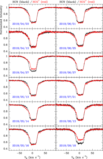
Figure 2: Lines of HCO⁺ ($J=1-0$) and HCN ($J=1-0$) observed as part of our data (see Sect. 3).

Appendix B Spectroscopic and observational line parameters

Tables 3 $-$ 11 show spectroscopic and observational line parameters for the detected species.

Table 3: Line parameters of CH₃SH.

Transition	$\nu_{\rm rest}$	$\nu_{\rm z=0.885875}$	$E_{\rm u}$/$k_{\rm B}$	$A_{\rm ul}$	$S_{\rm ul}\,\mu_{\rm a}^{2}$	$g_{\rm u}$	$\displaystyle{\int}\tau dv$	$v_{\rm 0}$	$v_{\rm FWHM}$
$(J_{K})_{\rm u}\rightarrow(J_{K})_{\rm l}$	[MHz]	[MHz]	[K]	[s-1]			[10-3 km s-1]	[km s-1]	[km s-1]
A, 3${}_{1}^{+}$ $\rightarrow$ 2${}_{1}^{+}$	75085.910	39814.892	8.6	3.24 $\times$ 10-6	4.60	7	30 (5)	$-$0.8 (0.9)	11 (2)
A, 3${}_{0}^{+}$ $\rightarrow$ 2${}_{0}^{+}$	75862.870	40226.881	5.1	3.75 $\times$ 10-6	5.17	7	}24mm[ 85 (8)$\dagger$]	$-$0.7 (0.5)	12 (1)
E, 30 $\rightarrow$ 20	75864.430	40227.709	5.2	3.76 $\times$ 10-6	5.18	7
E, 31 $\rightarrow$ 21	75925.910	40260.309	8.4	3.35 $\times$ 10-6	4.60	7	8 (3)	$-$1.8 (0.4)	2.4 (0.7)

Table 4: Line parameters of l-C₃H⁺.

Transition	$\nu_{\rm rest}$	$\nu_{\rm z=0.885875}$	$E_{\rm u}$/$k_{\rm B}$	$A_{\rm ul}$	$S_{\rm ul}$	$g_{\rm u}$	$\displaystyle{\int}\tau dv$	$v_{\rm 0}$	$v_{\rm FWHM}$
$J_{\rm u}\rightarrow J_{\rm l}$	[MHz]	[MHz]	[K]	[s-1]			[10-3 km s-1]	[km s-1]	[km s-1]
2 $\rightarrow$ 1	44979.544	23850.756	3.2	3.81 $\times$ 10-6	2.0	5	57 (8)	$-$0.5 (0.4)	5.4 (0.8)
3 $\rightarrow$ 2	67468.856	35775.890	6.5	1.38 $\times$ 10-5	3.0	7	84 (10)	$-$0.6 (0.2)	7.0 (0.9)
4 $\rightarrow$ 3	89957.617	47700.731	10.8	3.39 $\times$ 10-5	4.0	9	55 (6)	$-$0.8 (0.3)	4.5 (0.5)

Table 5: Line parameters of C₃N.

Transition	$\nu_{\rm rest}$	$\nu_{\rm z=0.885875}$	$E_{\rm u}$/$k_{\rm B}$	$A_{\rm ul}$	$S_{\rm ul}$	$g_{\rm u}$	$\displaystyle{\int}\tau dv$	$v_{\rm 0}$	$v_{\rm FWHM}$
$(N,J,F)_{\rm u}\rightarrow(N,J,F)_{\rm l}$	[MHz]	[MHz]	[K]	[s-1]			[10-3 km s-1]	[km s-1]	[km s-1]
${\mathrm{(6,13/2,13/2)\rightarrow(5,11/2,13/2)}}$	59361.053	31476.664	10.0	2.18 $\times$ 10-7	0.15	14	}6.5*[55 (5)$\dagger$]	$-$0.5 (0.2)	7.8 (0.7)
${\mathrm{(6,13/2,11/2)\rightarrow(5,11/2,9/2)\,\,\,}}$	59361.383	31476.839	10.0	8.87 $\times$ 10-6	5.38	12
${\mathrm{(6,13/2,13/2)\rightarrow(5,11/2,11/2)}}$	59361.386	31476.840	10.0	8.91 $\times$ 10-6	6.31	14
${\mathrm{(6,13/2,15/2)\rightarrow(5,11/2,13/2)}}$	59361.418	31476.857	10.0	9.13 $\times$ 10-6	7.38	16
${\mathrm{(6,13/2,11/2)\rightarrow(5,11/2,11/2)}}$	59364.084	31478.271	10.0	2.53 $\times$ 10-7	0.15	12
${\mathrm{(6,11/2,11/2)\rightarrow(5,9/2,11/2)\,\,\,}}$	59377.528	31485.400	10.0	2.95 $\times$ 10-7	0.18	12	}6.5*[(a)]
${\mathrm{(6,11/2,9/2)\rightarrow(5,9/2,7/2)\,\,\,}}$	59380.159	31486.795	10.0	8.64 $\times$ 10-6	4.36	10
${\mathrm{(6,11/2,11/2)\rightarrow(5,9/2,9/2)\,\,\,\,\,\,}}$	59380.192	31486.812	10.0	8.70 $\times$ 10-6	5.27	12
${\mathrm{(6,11/2,13/2)\rightarrow(5,9/2,11/2)\,\,\,}}$	59380.194	31486.813	10.0	9.00 $\times$ 10-6	6.36	14
${\mathrm{(6,11/2,9/2)\rightarrow(5,9/2,9/2)\,\,\,}}$	59380.912	31487.194	10.0	3.56 $\times$ 10-7	0.18	10
${\mathrm{(7,15/2,15/2)\rightarrow(6,13/2,15/2)}}$	69255.887	36723.477	13.3	2.62 $\times$ 10-7	0.13	16	}6.5*[26 (3)$\dagger$]	$-$0.8 (0.2)	4.2 (0.5)
${\mathrm{(7,15/2,13/2)\rightarrow(6,13/2,11/2)}}$	69256.249	36723.669	13.3	1.44 $\times$ 10-5	6.40	14
${\mathrm{(7,15/2,15/2)\rightarrow(6,13/2,13/2)}}$	69256.252	36723.670	13.3	1.44 $\times$ 10-5	7.33	16
${\mathrm{(7,15/2,17/2)\rightarrow(6,13/2,15/2)}}$	69256.275	36723.683	13.3	1.47 $\times$ 10-5	8.40	18
${\mathrm{(7,15/2,13/2)\rightarrow(6,13/2,13/2)}}$	69258.947	36725.099	13.3	2.99 $\times$ 10-7	0.13	14
${\mathrm{(7,13/2,13/2)\rightarrow(6,11/2,13/2)}}$	69272.375	36732.220	13.3	3.41 $\times$ 10-7	0.15	14	}6.5*[20 (3)$\dagger$]	$-$1.5 (0.2)	3.9 (0.7)
${\mathrm{(7,13/2,11/2)\rightarrow(6,11/2,9/2)\,\,\,}}$	69275.018	36733.621	13.3	1.41 $\times$ 10-5	5.38	12
${\mathrm{(7,13/2,13/2)\rightarrow(6,11/2,11/2)}}$	69275.042	36733.634	13.3	1.42 $\times$ 10-5	6.31	14
${\mathrm{(7,13/2,15/2)\rightarrow(6,11/2,13/2)}}$	69275.044	36733.635	13.3	1.45 $\times$ 10-5	7.39	16
${\mathrm{(7,13/2,11/2)\rightarrow(6,11/2,11/2)}}$	69275.738	36734.003	13.3	3.99 $\times$ 10-7	0.15	12
${\mathrm{(8,17/2,17/2)\rightarrow(7,15/2,17/2)}}$	79150.600	41970.226	17.1	3.07 $\times$ 10-7	0.12	18	}6.5*[(b)]
${\mathrm{(8,17/2,15/2)\rightarrow(7,15/2,13/2)}}$	79150.986	41970.431	17.1	2.17 $\times$ 10-5	7.41	16
${\mathrm{(8,17/2,17/2)\rightarrow(7,15/2,15/2)}}$	79150.988	41970.432	17.1	2.18 $\times$ 10-5	8.35	18
${\mathrm{(8,17/2,18/2)\rightarrow(7,15/2,17/2)}}$	79151.006	41970.441	17.1	2.21 $\times$ 10-5	9.41	20
${\mathrm{(8,17/2,15/2)\rightarrow(7,15/2,15/2)}}$	79153.682	41971.860	17.1	3.45 $\times$ 10-7	0.12	16
${\mathrm{(8,15/2,15/2)\rightarrow(7,13/2,15/2)}}$	79167.099	41978.975	17.1	3.87 $\times$ 10-7	0.13	16	}6.5*[19 (4)$\dagger$]	0.3 (0.5)	5 (1)
${\mathrm{(8,15/2,13/2)\rightarrow(7,13/2,11/2)}}$	79169.750	41980.380	17.1	2.15 $\times$ 10-5	6.40	14
${\mathrm{(8,15/2,15/2)\rightarrow(7,13/2,13/2)}}$	79169.768	41980.390	17.1	2.15 $\times$ 10-5	7.33	16
${\mathrm{(8,15/2,17/2)\rightarrow(7,13/2,15/2)}}$	79169.770	41980.391	17.1	2.19 $\times$ 10-5	8.40	18
${\mathrm{(8,15/2,13/2)\rightarrow(7,13/2,13/2)}}$	79170.446	41980.750	17.1	4.44 $\times$ 10-7	0.13	14

Table 6: Line parameters of HCOOH.

Transition	$\nu_{\rm rest}$	$\nu_{\rm z=0.885875}$	$E_{\rm u}$/$k_{\rm B}$	$A_{\rm ul}$	$S_{\rm ul}$	$g_{\rm u}$	$\displaystyle{\int}\tau dv$	$v_{\rm 0}$	$v_{\rm FWHM}$
$(J_{K_{\rm a},K_{\rm c}})_{\rm u}\rightarrow(J_{K_{\rm a},K_{\rm c}})_{\rm l}$	[MHz]	[MHz]	[K]	[s-1]			[10-3 km s-1]	[km s-1]	[km s-1]
31,3 $\rightarrow$ 21,2	64936.268	34432.965	9.4	2.45 $\times$ 10-6	2.67	7	39 (4)	$-$1.0 (0.2)	5.3 (0.6)
30,3 $\rightarrow$ 20,2	67291.121	35681.645	6.5	3.07 $\times$ 10-6	3.00	7	34 (3)	$-$0.7 (0.2)	4.2 (0.4)
31,2 $\rightarrow$ 21,1	69851.954	37039.546	9.9	3.05 $\times$ 10-6	2.67	7	42 (2)	$-$0.6 (0.2)	6.1 (0.5)
41,4 $\rightarrow$ 31,3	86546.180	45891.790	13.6	6.35 $\times$ 10-6	3.75	9	38 (8)	$-$0.6 (0.7)	6 (1)
40,4 $\rightarrow$ 30,3	89579.168	47500.056	10.8	7.51 $\times$ 10-6	4.00	9	27 (6)	$-$0.9 (0.4)	2.8 (0.6)

Table 7: Line parameters of CH₂CHCN.

Transition	$\nu_{\rm rest}$	$\nu_{\rm z=0.885875}$	$E_{\rm u}$/$k_{\rm B}$	$A_{\rm ul}$	$S_{\rm ul}$	$g_{\rm u}$	$\displaystyle{\int}\tau dv$	$v_{\rm 0}$	$v_{\rm FWHM}$
$(J_{K_{\rm a},K_{\rm c}})_{\rm u}\rightarrow(J_{K_{\rm a},K_{\rm c}})_{\rm l}$	[MHz]	[MHz]	[K]	[s-1]			[10-3 km s-1]	[km s-1]	[km s-1]
71,7 $\rightarrow$ 61,6	64749.012	34333.671	14.6	2.11 $\times$ 10-5	6.86	15	26.1 (3.2)	$-$0.2 (0.4)	5.7 (0.7)
70,7 $\rightarrow$ 60,6	66198.347	35102.193	12.7	2.30 $\times$ 10-5	7.00	15	26.7 (3.5)	$-$0.6 (0.3)	6.3 (0.8)
71,6 $\rightarrow$ 61,5	67946.687	36029.263	15.2	2.44 $\times$ 10-5	6.86	15	28.6 (4.4)	$-$0.9 (0.4)	6.1 (0.9)
81,8 $\rightarrow$ 71,7	73981.555	39229.299	18.2	3.19 $\times$ 10-5	7.87	17	21.5 (3.2)	$-$2.2 (0.3)	5.0 (0.8)$\dagger$
80,8 $\rightarrow$ 70,7	75585.693	40079.906	16.4	3.45 $\times$ 10-5	8.00	17	24.3 (3.6)	$-$0.2 (0.4)	5.0 (0.8)$\dagger$
82,6 $\rightarrow$ 72,5	76128.883	40367.937	25.1	3.31 $\times$ 10-5	7.50	17	5.6 (0.8)	$-$1.5 (0.7)	5.0 (0.8)$\dagger$,$\dagger$$\dagger$
81,7 $\rightarrow$ 71,6	77633.824	41165.944	18.9	3.68 $\times$ 10-5	7.87	17	16.8 (2.9)	$+$0.3 (0.4)	5.0 (0.8)$\dagger$,$\dagger$$\dagger$

Table 8: Line parameters of o-H₂CN.

Transition	$\nu_{\rm rest}$	$\nu_{\rm z=0.885875}$	$E_{\rm u}$/$k_{\rm B}$	$A_{\rm ul}$	$S_{\rm ul}$	$g_{\rm u}$	$\displaystyle{\int}\tau dv$	$v_{\rm 0}$	$v_{\rm FWHM}$
$(N_{K_{\rm a},K_{\rm c}},n,F)_{\rm u}\rightarrow(N_{K_{\rm a},K_{\rm c}},n,F)_{\rm l}$	[MHz]	[MHz]	[K]	[s-1]			[10-3 km s-1]	[km s-1]	[km s-1]
(10,1, 3, 5/2) $\rightarrow$ (00,0, 2, 3/2)	73345.486	38892.019	3.5	2.83 $\times$ 10-6	0.57	6	15 (4)	$-$1.7 (0.6)	4 (1)
(10,1, 0, 7/2) $\rightarrow$ (00,0, 0, 5/2)	73349.648	38894.226	3.5	3.29 $\times$ 10-6	0.89	8	20 (6)	$-$0.4 (0.4)	4 (1)
(10,1, 2, 5/2) $\rightarrow$ (00,0, 3, 3/2)	73409.042	38925.720	3.5	3.17 $\times$ 10-6	0.64	6	22 (6)	$-$1.0 (0.6)	4 (1)
(10,1, 4, 5/2) $\rightarrow$ (00,0, 0, 5/2)	73444.240	38944.384	3.5	2.73 $\times$ 10-6	0.55	6	15 (4)	$-$0.4 (0.8)	6 (2)

Table 9: Line parameters of OCS.

Transition	$\nu_{\rm rest}$	$\nu_{\rm z=0.885875}$	$E_{\rm u}$/$k_{\rm B}$	$A_{\rm ul}$	$S_{\rm ul}$	$g_{\rm u}$	$\displaystyle{\int}\tau dv$	$v_{\rm 0}$	$v_{\rm FWHM}$
$J_{\rm u}\rightarrow J_{\rm l}$	[MHz]	[MHz]	[K]	[s-1]			[10-3 km s-1]	[km s-1]	[km s-1]
5 $\rightarrow$ 4	60814.270	32247.244	8.8	6.09 $\times$ 10-7	5.0	11	52 (4)	$-$0.8 (0.1)	5.4 (0.4)
6 $\rightarrow$ 5	72976.781	38696.510	12.3	1.07 $\times$ 10-6	6.0	13	66 (4)	$-$0.8 (0.1)	5.8 (0.4)
7 $\rightarrow$ 6	85139.104	45145.677	16.3	1.71 $\times$ 10-6	7.0	15	42 (10)	$-$0.7 (0.8)	6 (1)

Table 10: Line parameters of SO₂.

Transition	$\nu_{\rm rest}$	$\nu_{\rm z=0.885875}$	$E_{\rm u}$/$k_{\rm B}$	$A_{\rm ul}$	$S_{\rm ul}$	$g_{\rm u}$	$\displaystyle{\int}\tau dv$	$v_{\rm 0}$	$v_{\rm FWHM}$
$(J_{K_{\rm a},K_{\rm c}})_{\rm u}\rightarrow(J_{K_{\rm a},K_{\rm c}})_{\rm l}$	[MHz]	[MHz]	[K]	[s-1]			[10-3 km s-1]	[km s-1]	[km s-1]
41,3 $\rightarrow$ 40,4	59224.870	31404.452	12.0	3.01 $\times$ 10-6	4.20	9	86 (3)	$-$0.9 (0.1)	6.8 (0.3)
61,5 $\rightarrow$ 60,6	68972.159	36573.028	22.5	4.34 $\times$ 10-6	5.54	13	49 (5)	$-$0.7 (0.3)	8.3 (0.8)
11,1 $\rightarrow$ 00,0	69575.929	36893.182	3.3	3.49 $\times$ 10-6	1.00	3	90 (5)	$-$1.0 (0.1)	6.7 (0.4)

Table 11: Line parameters of NH₂CN.

Transition	$\nu_{\rm rest}$	$\nu_{\rm z=0.885875}$	$E_{\rm u}$/$k_{\rm B}$	$A_{\rm ul}$	$S_{\rm ul}$	$g_{\rm u}$	$\displaystyle{\int}\tau dv$	$v_{\rm 0}$	$v_{\rm FWHM}$
$(J_{K_{\rm a},K_{\rm c}})_{\rm u}\rightarrow(J_{K_{\rm a},K_{\rm c}})_{\rm l}$	[MHz]	[MHz]	[K]	[s-1]			[10-3 km s-1]	[km s-1]	[km s-1]
O+, 31,3 $\rightarrow$ 21,2	59587.700	31596.845	20.2	1.76 $\times$ 10-5	8.00	21	30 (3)	$-$0.7 (0.3)	7.2 (0.7)
O+, 30,3 $\rightarrow$ 20,2	59985.700	31807.888	5.8	2.02 $\times$ 10-5	3.00	7	16 (3)	$-$1.4 (0.7)	7.0 (1.0)$\dagger$
O+, 31,2 $\rightarrow$ 21,1	60378.911	32016.391	20.3	1.83 $\times$ 10-5	8.00	21	34 (4)	$-$0.4 (0.3)	7.4 (0.9)
O+, 41,4 $\rightarrow$ 31,3	79449.729	42128.842	24.0	4.55 $\times$ 10-5	11.25	27	43 (5)	$-$1.2 (0.3)	6.0 (0.7)
O+, 40,4 $\rightarrow$ 30,3	79979.596	42409.808	9.6	4.95 $\times$ 10-5	4.00	9	30 (4)	$-$1.4 (1.2)	7.0 (1.0)$\dagger$
O+, 41,3 $\rightarrow$ 31,2	80504.600	42688.195	24.2	4.74 $\times$ 10-5	11.25	27	48 (6)	$-$0.4 (0.3)	6.6 (0.9)

Appendix C Rotational diagrams

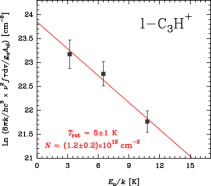
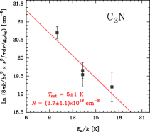
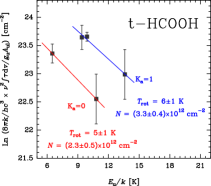
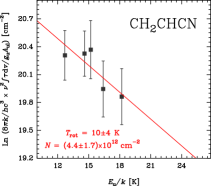
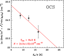
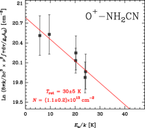
Figure 3: Rotational diagrams of the detected molecules towards PKS 1830$-$211. Derived values of the rotational temperature, $T_{\rm rot}$, column density, $N$, and their respective uncertainties are also indicated for each molecule.

As we detected several molecules in more than one transition, we can estimate rotational temperatures ($T_{\rm rot}$) and molecular column densities ($N$) for the detected species by constructing rotational diagrams (see e.g. Goldsmith & Langer 1999). This analysis assumes the Rayleigh-Jeans approximation, optically thin lines, and LTE conditions. The equation that derives the total column density under these conditions can be re-arranged as

$${\rm\ln}\left(\frac{8\pi k_{\rm B}\nu^{2}\int{\tau_{\rm\nu}dv}}{hc^{3}A_{\rm ul}g_{\rm u}}\right)={\rm\ln}\left(\frac{N}{Q_{\rm rot}T_{\rm rot}}\right)-\frac{E_{\rm u}}{k_{\rm B}T_{\rm rot}},$$ (2)

where $g_{u}$ is the statistical weight in the upper level, $A_{\rm ul}$ is the Einstein A-coefficient for spontaneous emission, $Q_{\rm rot}$ is the rotational partition function which depends on $T_{\rm rot}$, $E_{\rm u}$ is the upper level energy, and $\nu$ is the frequency of the transition. We obtained the integrated opacity of the line, $\int{\tau_{\rm\nu}dv}$, by multiplying $\tau_{\rm\nu}$ by $v_{\rm FWHM}$.

The first term of Eq. 2, which only depends on spectroscopic and observational line parameters, is plotted as a function of $E_{\rm u}$/$k_{\rm B}$ for the different detected lines. Thus, the $T_{\rm rot}$ and $N$ can be derived by performing a linear least square fit to the points (see Fig. 3). Although we detected four lines of H₂CN, it is not possible to perform a rotational diagram for this species since these lines correspond to different hyperfine structure transitions with equal ($N_{K_{\rm a},K_{\rm c}}$)_u $\rightarrow$ ($N_{K_{\rm a},K_{\rm c}}$)_l state (and also equal $E_{\rm u}$/$k_{\rm B}$, see Table 8).

Under the conditions of a subthermally excited gas, the rotational population diagram of symmetric- and asymmetric-top molecules such as HCOOH shows separate rotational ladders for each set of transitions with the same $K_{\rm a}$ quantum number. For very polar molecules, subthermal excitation happens at relatively high densities. Therefore, accurate column densities and rotational temperatures from rotational diagrams can only be obtained if the individual column densities for each rotational ladder are computed independently (see Cuadrado et al. 2016, 2017). This effect has also prevented the analysis of the CH₃SH lines since we have only detected one line with $K_{\rm a}$ = 0 and another with $K_{\rm a}$ = 1 per state (A/E).

For HCOOH, we built specific rotational diagrams for different sets of lines with the same $K_{\rm a}$ quantum number. The total column density of the molecule is obtained by adding the column density of each rotational ladder. CH₂CHCN shows a similar tendency. However, due to the large uncertainties of the individual points and the limited number of observed transitions, we performed the rotational diagram from a single linear least square fitting. For the other molecules, it is possible to fit the lines from different $K$-ladders by a single $T_{\rm rot}$ and $N$.

Due to the reduced number of rotational transitions, the rotational diagram of O⁺-NH₂CN (the lower inversion state of NH₂CN) was built by taking the different statistical weights for the $ortho$ ($K_{\rm a}$ = 1) and $para$ ($K_{\rm a}$ = 0) states into account (see $g_{\rm u}$ in Table 11). Interestingly, the rotational diagram of the very polar and asymmetric-top NH₂CN shows the points of different $K_{\rm a}$ ladders merging in a single straight line. This characteristic straight diagram is typically seen towards high density regions, such as hot cores (see e.g. López et al. 2014). For this kind of species, this merging of the $K_{\rm a}$ ladders only occurs at very high gas densities, which are higher than the critical density for collisional excitation.

For C₃N, different hyperfine structure components of the same ($N$, $F$)_u $\rightarrow$ ($N$, $F$)_l transition are blended in a single line. Thus, to correctly determine $T_{\rm rot}$ and $N$, the line strength ($S_{\rm ul}$) was calculated as the sum of all allowed hyperfine components of each ($N$, $F$)_u $\rightarrow$ ($N$, $F$)_l transition. The characteristic frequency ($\nu$) was determined using the weighted average with the relative strength of each line as weight and $A_{\rm ul}$ was calculated using these derived values.

Results for $T_{\rm rot}$ and $N$ using the population diagram procedure are shown in Table 1 and Fig. 3. The uncertainties were calculated using the statistical errors given by the linear least squares fit for the slope and the intercept. The individual errors of the data points are those derived by taking into account the uncertainty obtained in the determination of the observed line parameters (see Tables 3 $-$ 11).