Fusing Online Gaussian Process-Based Learning and Control for Scanning Quantum Dot Microscopy

Abstract

Elucidating electrostatic surface potentials contributes to a deeper understanding of the nature of matter and its physicochemical properties, which is the basis for a wide field of applications. Scanning quantum dot microscopy, a recently developed technique allows to measure such potentials with atomic resolution. For an efficient deployment in scientific practice, however, it is essential to speed up the scanning process. To this end we employ a two-degree-of-freedom control paradigm, in which a Gaussian process is used as the feedforward part. We present a tailored online learning scheme of the Gaussian process, adapted to scanning quantum dot microscopy, that includes hyperparameter optimization during operation to enable fast and precise scanning of arbitrary surface structures. For the potential application in practice, the accompanying computational cost is reduced evaluating different sparse approximation approaches. The fully independent training conditional approximation, used on a reduced set of active training data, is found to be the most promising approach.

I Introduction

Research in physical chemistry and nanotechnology is driven by a wide field of possible future applications such as, for instance, molecular manipulation that enables the assembly of molecular machines or nanoscopic electric circuits by single molecule placement [1, 2]. This research requires a fundamental understanding of the basic building blocks of matter, atoms and molecules. Therein, imaging of nanostructures plays an important role.

Visualizing surface nanostructures can be accomplished using scanning probe microscopy techniques [3]. One such recently developed technique is scanning quantum dot microscopy (SQDM) [4, 5] that probes the electrostatic potential of a surface structure using a single molecule as sensor. It provides qualitative and quantitative images of the electrostatic potentials of nanostructures on surfaces with atomic resolution as shown in Fig. 1.

Despite SQDM’s large potential, widespread deployment in scientific practice was initially hindered due to excessive scan times. To accelerate the scanning process a tailored two-degree-of-freedom (2DOF) controller, comprising a feedback and feedforward controller, was developed [5]. The feedforward part is utilized to generate a prediction for upcoming measurement points. The feedback part corrects the discrepancies between the real and the predicted measurement values. So far, the feedforward part that is implemented in the experiment uses the previously scanned line to generate a prediction for the next line. In [6] however, we could show in simulations that a better prediction can be obtained if a Gaussian process (GP) is used to generate the feedforward signal.

In this work we further develop the 2DOF controller with the GP towards real-time applicability for SQDM. To this end, two challenges in particular regarding the feedforward are elementary. First, so far, a priori knowledge of the involved hyperparameters of the GP was assumed to be available. Second, the necessary GP computations are expensive for real-time feasibility. To account for these challenges the contributions of this work are

1. online hyperparameter learning for SQDM such that no a priori knowledge is required,

2. verification of real-time capability via preselection, comparison, and adaptation of different sparse GP approaches for computational reduction, and

3. verification of the selected approaches and their potential real-time feasibility in SQDM control.

One of the main messages of this paper is that the fusion of control with learning enables new and improved applications, such as SQDM.

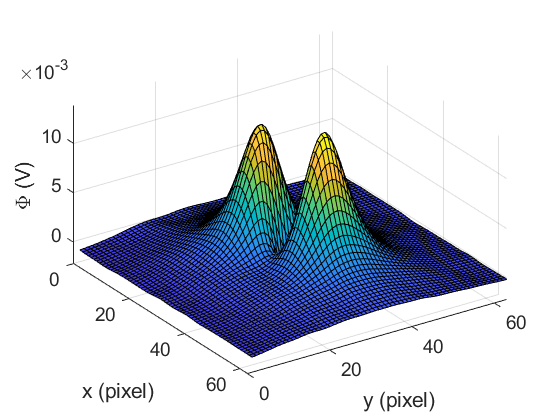
Figure 1: SQDM image of a single molecule [4].

The structure of the remainder of this paper is as follows. We outline the working principle of SQDM in Section II. In Section III, we introduce the 2DOF control paradigm for SQDM including a brief overview of GPs. In Section IV, we present the sparse GP approaches compared in this work. The simulation results are shown in Section V and we draw conclusions in Section VI.

II Scanning Quantum Dot Microscopy

SQDM generates images of electrostatic potentials of nanostructures on surfaces with nanometer resolution. To this end it utilizes a sensor molecule denoted as quantum dot (QD) [4, 5], which is bonded to the tuning fork of a frequency modulated non-contact atomic force microscope (NC-AFM). Between the sample and the tip a bias voltage source $V_{\text{b}}$ is connected (Fig. 2a) that generates an electrostatic potential, which is superimposed to that of the sample.

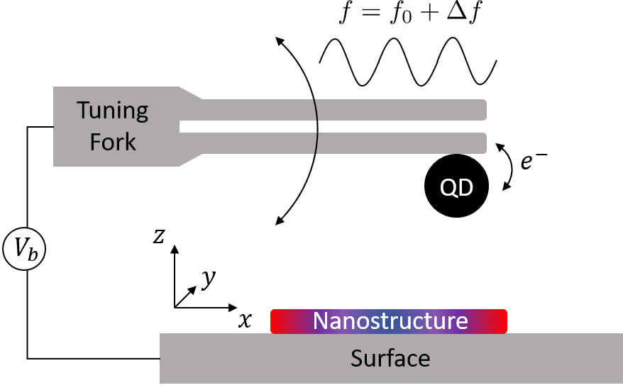
(a)

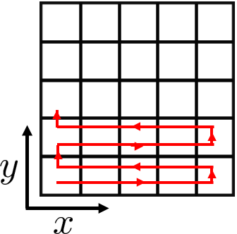
(b)

Figure 2: (a): Schematic set-up of scanning quantum dot microscopy (adapted from [6]). (b): Raster scan pattern. The image is divided into pixels. Lines are indexed by $y$, columns by $x$. The red arrows indicate scanning direction.

While performing a raster scan pattern (Fig. 2b), $V_{\text{b}}$ is varied. If the effective potential at the QD reaches specific thresholds, the QD is charged or discharged via electron tunneling between the microscope tip and the QD. These charging events lead to abrupt changes in the tuning fork’s oscillation frequency, sensed by the NC-AFM, and appear in the spectrum $\Delta f(V_{\text{b}})$ as features, called dips (Fig. 3). The two occurring dips, one at negative voltages and one at positive voltages, are characterized by their respective position in the spectrum, indicated by their minima $V^{-}$ and $V^{+}$, or $V^{\mp}$ for short. The $V^{\mp}(r)$ values change with the tip position $r=(x,y,z)$ and are the main measurements of SQDM, which are then used in a post-processing step to determine the electrostatic potential of the sample [5, 7]. Note that the sample has to be scanned twice because the $V^{\mp}(r)$ data can be obtained only separately.

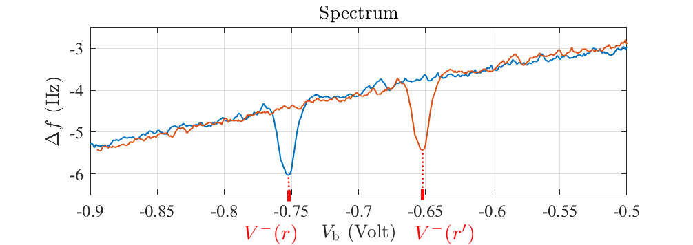
Figure 3: Exemplary cutout of the spectrum $\Delta f(V_{\text{b}})$ illustrating the movement of the negative dip at two microscope tip positions $r$ and $r^{\prime}$. Each plotted spectrum belongs to one specific tip position. For an illustration of the complete spectrum with both dips, see [6].

The challenge of SQDM imaging lies in the a priori unknown and changing voltage values $V^{\mp}(r)$ during scanning, which depend both on the sample’s topography, as well as its electric properties. Originally, the $V^{\mp}(r)$ values were determined by varying $V_{\text{b}}$ in a broad interval at each image pixel, which results in excessive scan times. This problem can be circumvented by employing a tailored two-degree-of-freedom control approach that continuously adapts $V_{\text{b}}$ to directly track the dips [6].

III Two-Degree-Of-Freedom Control of SQDM

In this section, we first outline the 2DOF control paradigm and its application to SQDM. Secondly, we give a brief overview of Gaussian processes including hyperparameter optimization.

III-A 2DOF Control Paradigm

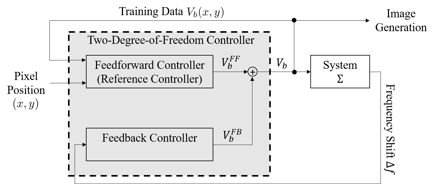
Figure 4: Diagram of the SQDM two-degree-of-freedom controller. The system $\Sigma$ represents the NC-AFM. The frequency shift $\Delta f$ of the NC-AFM is the feedback signal for the feedback controller, c.f. [6].

The two-degree-of-freedom controller as presented in [6] consists of a feedback and a feedforward part (Fig. 4). The feedback controller is an extremum seeking controller [8] that allows to directly track the dips and with that the $V^{\mp}(r)$ values. It continuously adjusts $V_{\text{b}}$ such that the respective dip is minimized [6], i.e.,

$$V^{-}(r) =\operatorname*{arg\,min}_{V_{\text{b}}<0}\Delta f(V_{\text{b}},r)$$ (1)

$$V^{+}(r) =\operatorname*{arg\,min}_{V_{\text{b}}>0}\Delta f(V_{\text{b}},r)\ .$$

Tracking of the dips with the extremum seeking controller works only as long as the current $V_{\text{b}}$ value is within the respective dip. If one of the dips changes its position faster (see Fig. 3) than the feedback controller is able to follow, then $V_{\text{b}}$ leaves the dip and scanning has to be aborted. To prevent this, the feedforward part, which is based on a Gaussian process, generates a prediction $V_{\text{b}}^{\text{FF}}$ of the respective $V^{\mp}(r)$ evolution for the next line, which is added to the $V_{\text{b}}$ output of the feedback controller $V_{\text{b}}^{\text{FB}}$. Thus, the feedforward signal has to be as accurate as possible and is critical for correct operation. The remainder of this work will be focused therefore on using Gaussian process based learning to obtain the feedforward signal $V_{\text{b}}^{\text{FF}}$ for the next line, based on the data of previous lines.

III-B Gaussian Process Regression

A Gaussian process $f(\xi)\sim\mathcal{GP}(m(\xi),k(\xi,\xi^{\prime}))$ can be used to model a function $f:\mathbb{R}^{t}\rightarrow\mathbb{R}^{s},\xi\mapsto f(\xi)$. In this work it will be used to model the feedforward signal with the tip position $\xi=r=(x,y)$ as input and the respective output $f(\xi)=V^{\mp}$. Formally, a Gaussian processes is defined as a collection of random variables, any finite number of which have consistent joint Gaussian distributions [9]. That means, loosely speaking, that one might think of a Gaussian process as being an infinite-dimensional, multivariate normal distribution where the function values $f(\xi)$ are random values evaluated at the inputs $\xi$. A GP is fully defined by its mean function $m(\xi)=E[f(\xi)]$ ($E[\cdot]$ denotes the expected value) and covariance function $k(\xi,\xi^{\prime})=\text{cov}[f(\xi),f(\xi^{\prime})]=E[(f(\xi)-m(\xi))(f(\xi^{\prime})-m(\xi^{\prime}))]$, which both depend on a set of so-called hyperparameters $\theta$ [10], [11].

The objective is to learn the function $f$ and compute at $n_{*}$ test inputs $\xi_{*}^{(j)},~{}j=1,...,n_{*}$ the corresponding, predicted test targets stored as a vector $f_{*}\in\mathbb{R}^{n_{*}}$. To this end, noisy training observations (training targets) $\gamma=f(\Xi)+\varepsilon$ are required, where $\Xi\in\mathbb{R}^{d\times n},\Xi=[\xi^{(1)},...,\xi^{(n)}]$ is the matrix storing $n$ $d$-dimensional training inputs, $f(\Xi)\in\mathbb{R}^{n}$ is the vector of the corresponding, noise-free function values and $\varepsilon\sim\mathcal{N}(0,\sigma^{2}_{\text{n}}\mathbb{I})$, with $\mathbb{I}$ being the identity matrix, models white Gaussian/normally distributed noise with variance $\sigma^{2}_{\text{n}}$. The training and test data points are assumed to be independently and identically distributed.

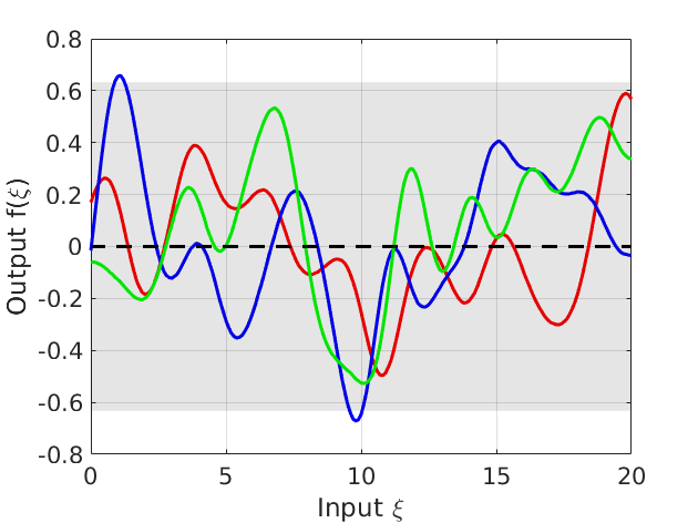
(a)

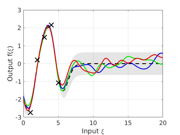
(b)

Figure 5: Illustration of GP inference. Functions drawn from a zero mean GP with isotropic squared exponential covariance function ($\sigma_{f}=0.1$, $\ell=1.0$). The grey-shaded area indicates the 95 % confidence interval. The dashed line shows the mean function. (a): Random functions drawn from the prior distribution. (b): Random functions drawn from the posterior distribution (2) with noise variance $\sigma^{2}_{\text{n}}=0.01$. Black crosses indicate training data.

To learn the function $f$, all prior functions (Fig. 5a) that cannot explain the measured training data set $\{\Xi,\gamma\}$ have to be rejected (Fig. 5b). This inference step is mathematically done by conditioning the prior on the training data (see [10]) to arrive at the posterior distribution $f_{*}\,|\,\Xi,\gamma,\Xi_{*}\sim\mathcal{N}(\bar{f}_{*},\hat{\sigma}^{2})$ with

$$\bar{f}_{*}\!=\!m_{\Xi_{*}}\!+\!K(\Xi_{*},\Xi)K_{\gamma}^{-1}K(\Xi,\Xi_{*})(\gamma\!-\!m_{\Xi})$$ (2a)

$$\hat{\sigma}^{2}\!=\!K_{*}\!-\!K(\Xi_{*},\Xi)K_{\gamma}^{-1}K(\Xi,\Xi_{*})\ ,$$ (2b)

where $\bar{f}_{*}\in\mathbb{R}^{n_{*}}$ is the posterior mean prediction and $\hat{\sigma}^{2}\in\mathbb{R}^{n_{*}\times n_{*}}$ is the predictive covariance matrix. Furthermore, $\Xi_{*}\in\mathbb{R}^{d\times n_{*}},\Xi_{*}=[\xi_{*}^{(1)},...,\xi_{*}^{(n_{*})}]$ is the matrix storing $n_{*}$ $d$-dimensional test inputs, $K(\cdot,\cdot)$ are covariance matrices, $K_{\gamma}=K(\Xi,\Xi)+\sigma^{2}_{\text{n}}\mathbb{I}$, $K_{*}=K(\Xi_{*},\Xi_{*})$, $m_{\Xi_{*}}=m(\Xi_{*})$ and $m_{\Xi}=m(\Xi)$.

Thus, the GP prediction used for the SQDM feedforward signal is computed by (2a), i.e., based on previous measurement pairs $\big{(}(x,y),V^{\mp}\big{)}$ the GP builds a model for $V^{\mp}(x,y)$ and generates a prediction for the next line $y+1$.

III-C Hyperparameter Adaptation

The GP mean and covariance function depend on a set of hyperparameters $\theta$ and hence, an appropriate GP prediction requires suitable hyperparameters. The optimal hyperparameters $\theta^{*}$ for a certain training data set $\{\Xi,\gamma\}$ can be obtained by maximizing the logarithmic likelihood

$$\text{log}\big{(}p(\gamma\,|\,\Xi,\theta)\big{)}=-\frac{1}{2}{\gamma_{0}}^{T}K_{\gamma}^{-1}\gamma_{0}\!-\!\frac{1}{2}\ln|K_{\gamma}|\!-\!\frac{n}{2}\ln(2\pi)~{},$$

where $p(\cdot)$ is the probability density function, $|\cdot|$ denotes the determinant and $\gamma_{0}=\gamma-m_{\Xi}$ is a standardization [10]. The logarithmic likelihood describes how well the training data is explained by the underlying model. The optimal hyperparameters are then

$$\theta^{*}=\arg\max_{\theta}\left\{\text{log}\big{(}p(\gamma\,|\,\Xi,\theta)\big{)}\right\}\ .$$ (3)

In SQDM, the training data is a continuously incoming stream of measurements. Therefore, hyperparameter optimization has to be performed online such that the GP model is capable of adequately describing the evolution of $V^{\mp}(r)$ in the current region of operation without a priori knowledge. This is computationally challenging because the computation time required for $K_{\gamma}^{-1}\in\mathbb{R}^{n\times n}$ scales in general with $\mathcal{O}(n^{3})$ [10].

IV Efficient Implementation of Gaussian Processes

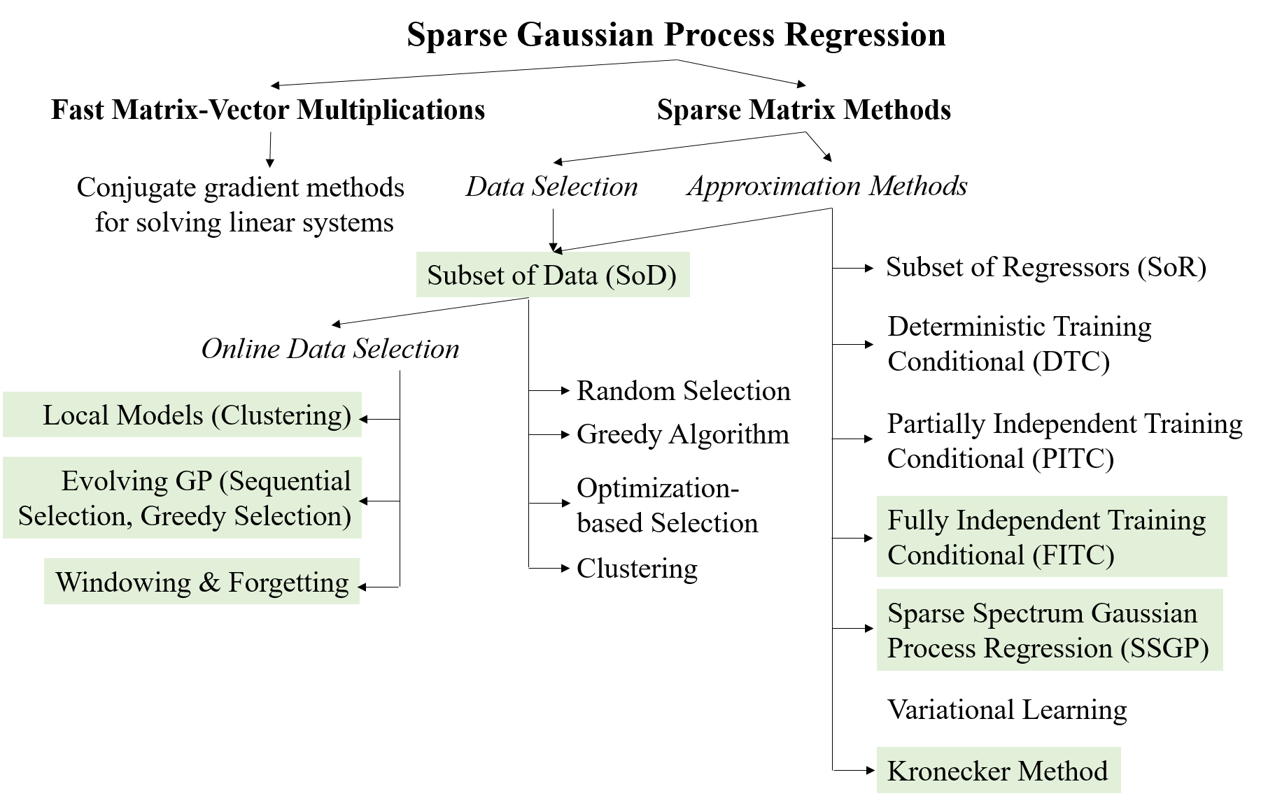
Figure 6: Overview of approaches for a sparse implementation of Gaussian processes. The ones selected for implementation and testing are highlighted.

Computing and adjusting the GP online is crucial for use in SQDM. To reduce the computational load, especially for hyperparameter optimization as mentioned in the previous section, we have identified suitable approaches in a literature review. Fig. 6 provides an overview of the identified approaches, while more detailed presentations can be found in [11] (overview), [12] (SSGP), [9] (overview), [10] (overview), [13] (clustering), [14] (SoR), [15] (DTC), [16] (FITC), [17] (variational learning) and [18] (structure exploiting approaches, especially Kronecker method). Four of the approaches have been selected as the most promising for application in SQDM control and are therefore outlined in the following.

IV-A Subset of Data

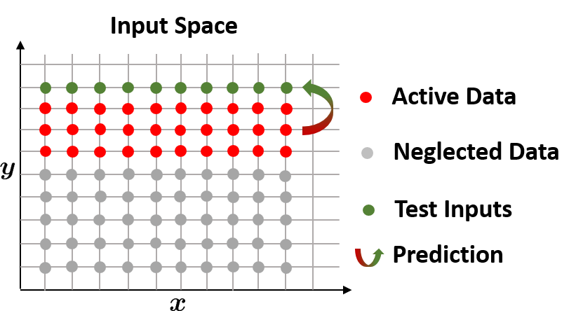
Figure 7: In the SoD approach, the prediction is based only on a subset of the available training data. Here, the sliding window approach for data selection is shown.

Instead of using the entire available training data, i.e., the training set $\mathcal{X}=\{\xi^{(j)},\gamma_{j}\}_{j=1}^{n}$, only a smaller subset of training data, the active set $\mathcal{I}=\{\xi^{(h)},\gamma_{h}\}_{h=1}^{n_{I}}$ of size $n_{I}\ll n$, is used in the SoD approach for GP modeling (Fig. 7). This reduces the computational complexity from $\mathcal{O}(n^{3})$ to $\mathcal{O}(n_{I}^{3})$ [9], [19]. Within this work, we use three different approaches outlined in the following for building the active set $\mathcal{I}$.

Sliding Window: The active set consists of the $n_{I}$ most recent data points [20].

Evolving GP: A new data point is included in $\mathcal{I}$ only if it provides new information to the current GP model, i.e., if the prediction error or the predictive variance exceed preset thresholds. Any time a new data point is included in $\mathcal{I}$, the point with the lowest information gain is removed [11]. For simplification, we just remove the oldest data point.

Clustering: The training data is clustered using the k-means algorithm (see [21]) with the covariance function as similarity measure. These clusters are then the active sets for distinct GP models [13].

IV-B Kronecker Method

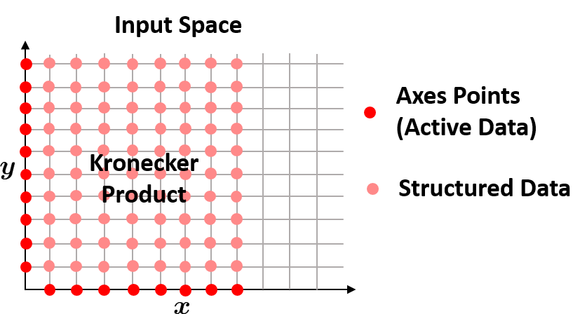
Figure 8: In the Kronecker method, the grid structure of the training data is exploited by using only the axes points as active points. The entire grid data is computed as Kronecker product.

The Kronecker method can only be applied if the inputs are points of a $D$-dimensional Cartesian grid and the covariance function $k$ has a product structure across grid dimensions. Exploiting the covariance function’s structure, it can be rewritten as $k(\xi,\xi^{\prime})=\prod_{d=1}^{D}k(\xi_{d},\xi^{\prime}_{d})$. Then, the covariance matrix $K\in\mathbb{R}^{n_{I}\times n_{I}}$, where $n_{I}$ is the number of grid points, can be computed using the Kronecker product $K=K_{1}\otimes...\otimes K_{D}$, where $K_{d}~{},~{}d=1,...,D$ is the covariance matrix of the points on the grid’s $d^{th}$ axis (Fig. 8). As a result of their smaller size, the Kronecker factors $K_{d}$ can be quickly eigendecomposed. From their eigendecompositions $K_{d}=Q_{d}V_{d}Q_{d}^{T}$, the eigendecomposition of $K$ can be efficiently computed as $K=QVQ^{T}$ with $Q=Q_{1}\otimes...\otimes Q_{D}$ and $V=V_{1}\otimes...\otimes V_{D}$. Therewith, computing the inverse $[K+\sigma^{2}_{\text{n}}\mathbb{I}]^{-1}$ becomes trivial and the computationally complexity reduces to $\mathcal{O}\left(Dn_{I}^{(1+\frac{1}{D})}\right)$ [18].

IV-C Fully Independent Training Conditional

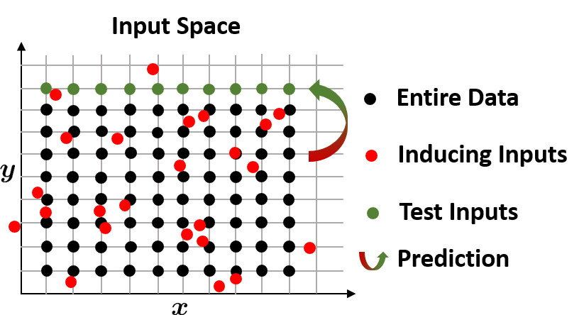
Figure 9: In the FITC approach, a small pseudo data set is used to explain the entire training data.

The Fully Independent Training Conditional (FITC) approximation is based on the idea to use a pseudo data set of $n_{I}\ll n$ inducing inputs stored in the matrix $I\in\mathbb{R}^{d\times n_{I}}$ and the corresponding observations $f_{I}\in\mathbb{R}^{n_{I}}$ to explain the training and test data (Fig. 9). There are two critical assumptions underlying the FITC approximation (see [9]), which we also adopt in this work. The first is that one assumes the training and test observations $\gamma$ and $f_{*}$ to be conditionally independent given $f_{I}$, i.e., that

$$p(f_{*},\gamma) =\int p(f_{*},\gamma,f_{I})\mathop{}\!\mathrm{d}f_{I}$$

$$=\int p(f_{*}\,|\,f_{I})p(\gamma\,|\,f_{I})p(f_{I})\mathop{}\!\mathrm{d}f_{I}~{}$$

holds. This means, loosely speaking, that the test and training variables are only connected indirectly via the inducing variables that induce their dependencies [9]. One might think of projecting the entire training variables onto the inducing variables and compute the test variables again as a projection of the inducing variables, such that the prediction is based on an approximate representation of the entire training data.

The second assumption affects the relationship between the training and the inducing variables described by the conditional $p(\gamma\,|\,f_{I})$. A fully independent conditional is assumed, i.e., the training variables are only self-dependent and thus, the covariance matrix has a diagonal structure. The approximate conditional $q(\gamma\,|\,f_{I})$ is then given by

$$q(\gamma\,|\,f_{I})\!=\!\mathcal{N}\left(m_{\Xi}\!+\!K(\Xi,I)K_{I}^{-1}f_{I,0}~{},~{}\text{diag}[K_{\gamma}\!-\!Q_{Xi}]\right),$$

where $Q_{\Xi}=K(\Xi,I)K_{I}^{-1}K(I,\Xi)$, $K_{I}=K(I,I)$ and $f_{I,0}=f_{I}-m(I)$ [9], [16]. Finally, the predictive distribution using FITC is

$$q_{\text{FITC}}(f_{*}\,|\,\gamma) =\mathcal{N}\left(\bar{f}_{*,\text{FITC}},\hat{\sigma}^{2}_{\text{FITC}}\right)$$

$$\bar{f}_{*,\text{FITC}} =m_{\Xi_{*}}\!+\!K(\Xi_{*},I)\Sigma K(I,\Xi)\Lambda^{-1}\gamma_{0}$$

$$\hat{\sigma}_{\text{FITC}}^{2} =K_{*}-Q_{*}+K(\Xi_{*},I)\Sigma K(I,\Xi_{*})~{},$$

where $\Sigma=\left[K_{I}+K(I,\Xi)\Lambda^{-1}K(\Xi,I)\right]^{-1}$, $\Lambda=\text{diag}[K_{\gamma}-Q(\Xi,\Xi)]$ and $Q_{*}=K(\Xi_{*},I)K_{I}^{-1}K(I,\Xi_{*})$ [9].

The inducing inputs can be considered as additional covariance hyperparameters and thus, they can be found optimization-based by solving (3) [9], [16].
The computational complexity of the FITC approximation is $\mathcal{O}(nn_{I}^{2})$ [9].

IV-D Sparse Spectrum Gaussian Process Regression

In Sparse Spectrum Gaussian Process Regression (SSGPR), the GP is Fourier transformed into the frequency domain in order to decompose it in a (infinite) set of oscillations, each with a certain frequency. Thus, SSGPR works with power spectra rather than with random functions directly. A power spectrum of the GP describes how strong each frequency contributes to it (Fig. 10).

The basic idea of SSGPR is now to approximate the GP’s power spectrum by a finite set of Dirac pulses with finite amplitude to sparsify its representation [12]. We therefore consider a trigonometric Bayesian regression model given by

$$f(\xi)=\sum_{r=1}^{n_{I}}a_{r}\cos(2\pi s_{r}^{T}\xi)+b_{r}\sin(2\pi s_{r}^{T}\xi)$$ (4)

with $a_{r}\sim\mathcal{N}\left(0,\frac{\sigma_{f}^{2}}{n_{I}}\right)$ and $b_{r}\sim\mathcal{N}\left(0,\frac{\sigma_{f}^{2}}{n_{I}}\right)$, where $a_{r}$ and $b_{r}$ are the amplitudes of the basis functions, $s_{r}$ is a vector of spectral frequencies, $n_{I}$ is the number of basis functions and $\sigma_{f}$ is a covariance hyperparameter (see Sec. V). Under these conditions, the distribution over functions is a zero-mean Gaussian with the stationary covariance function [12]

$$k(\xi,\xi^{\prime})=\frac{\sigma_{f}^{2}}{n_{I}}\sum_{r=1}^{n_{I}}\cos(2\pi s_{r}^{T}(\xi-\xi^{\prime}))~{}~{}.$$ (5)

The spectral frequencies are therefore additional covariance hyperparameters describing the positions of the Dirac pulses. In consequence, the spectral frequencies can be found optimization-based by maximizing the logarithmic likelihood (see (3)) [12]. That means that the spectral frequencies are selected given the training data and thus, we learn the power spectrum of the GP instead of its mean function. Although the standard representation of the predictive distribution and the logarithmic likelihood as given in Section III can be used in SSGPR, a more efficient one is provided in [12].

The computational complexity of SSGPR is $\mathcal{O}(nn_{I}^{2})$ [12].

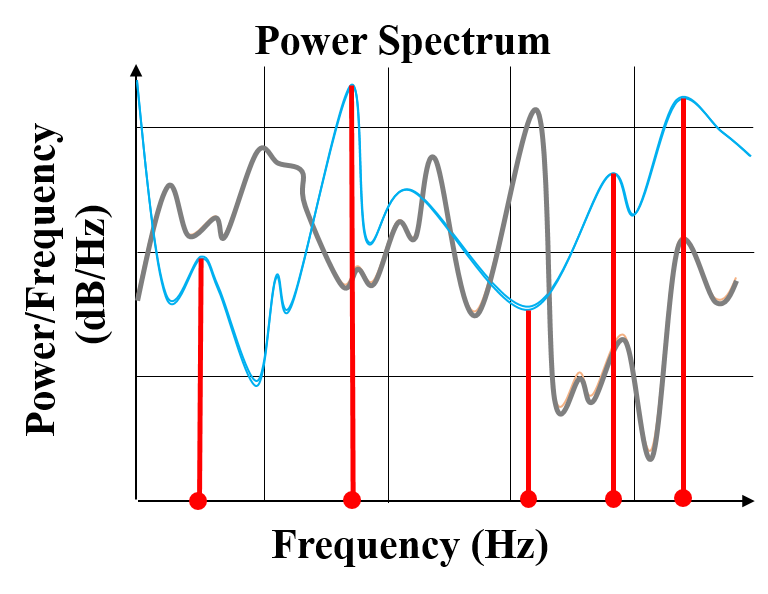
Figure 10: In SSGPR, the power spectrum of the GP is learned and sparsely represented by a finite set of Dirac pulses with finite amplitude.

V Implementation and Simulation Results

In this section, we first discuss the implementation of the online hyperparameter adaptation. Secondly, we show the simulation results for different reference images when using the sparse GP approaches presented in Section IV. Thirdly, we will investigate the computation times and practical applicability of the approaches.

V-A Preliminaries

We use a GP with constant mean function $m(\xi)=c$ with $c\in\mathbb{R}$. We tested several covariance functions of which the squared exponential (SE) covariance function $k(\xi_{p},\xi_{q})=\sigma_{f}^{2}\exp\left(-\frac{1}{2}(\xi_{p}-\xi_{q})^{T}M(\xi_{p}-\xi_{q})\right)$ worked best, with $M=\ell^{-2}\mathbb{I},\ell\in\mathbb{R}_{>0}$ for the isometric form (used for FITC and SSGPR) and $M=\text{diag}(\ell)^{-2},\ell\in\mathbb{R}^{D}_{>0}$ for the form with automatic relevance determination (used for SoD and the Kronecker method) and $\sigma_{f}\in\mathbb{R}_{>0}$ [10]. The algorithms used for implementation are geared towards the ones of the GPML toolbox [22].

During first evaluations we have found that FITC and SSGP work best on a reduced active training data set of the last five scanned lines and with one third of the number of training data as number of inducing inputs and spectral points respectively. For SoD and the Kronecker method, we use active sets of the size of two lines.

V-B Online Hyperparameter Adaptation

In order to make SQDM universally applicable, the controller has to have the ability of adapting to a specific experimental setting, e.g., arbitrary surface samples. In particular, the hyperparameters have to be adapted during scanning when no or only little prior knowledge on the scanned surface structure is available. Besides the hyperparameters’ dependency on the surface structure, they further depend on the physical properties of the quantum dot that is used for scanning. In addition, if the GP is sparsified using an inducing point method such as FITC, the number of inducing inputs should be chosen according to the amount of training data and thus, the number of hyperparameters depends in such case also on the size of the chosen raster pattern.

Hyperparameter adaptation is computed via (3) and implemented according to the following scheme. In a first step, the partial derivatives of the logarithmic likelihood w.r.t. the hyperparameters are computed. Additional prior knowledge on the hyperparameters can be included in the second step by correcting the derivatives due to the respective prior distributions. In a third step, the partial derivatives are then used in a conjugate gradient (CG) method with search direction computed according to Polak-Ribière (see [23]) to compute an estimate of the optimal hyperparameters. After the CG iteration has finished, the current estimate for the optimal hyperparameters is returned to the SQDM model (see [6]) and used for prediction.

As hyperparameter learning is computationally expensive, we have to approximate the GP using the approaches presented in Sec. IV in the next step to reduce computation to allow for online implementation.

V-C Comparison of Sparse GP Approaches

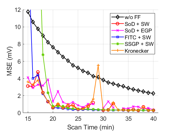
(a)

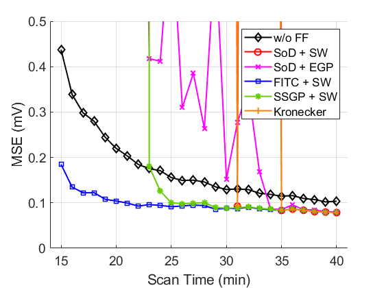
(b)

Figure 11: MSE for scanning R1 at different scan times. w/o FF: ESC only. SoD: Subset of Data. Kronecker: Kronecker method. FITC: Fully Independent Training Conditional. SSGP: Sparse Spectrum Gaussian Process. SW: Sliding Window. EGP: Evolving GP. (a): $V^{+}$ scan. Missing data points indicate an interruption of the simulation due to an error. (b): $V^{-}$ scan.

In order to compare the different sparse GP approaches, we simulate first the scans of the reference image of Fig. 1, denoted as R1 for different scan times. For each scan, we quantify the image quality using the mean-squared error (MSE) (see [24], [25]). For the sake of a better assessment of the results, we also show the MSE when using feedback control only.

We start with feedback control only. The MSE decreases monotonically with increasing scan time (Fig. 11). As the scan time increases the ESC has more time to converge to the true $V^{\mp}$ values, which explains this observation.

We continue with the SoD approach and the $V^{+}$ scan (Fig. 11a). The MSE shows no clear and consistent trend as a function of the scan time but increases and decreases by leaps and bounds. For the $V^{-}$ scan (Fig. 11b), long scan times are required for obtaining usable results. These are the same for either using the sliding window or the evolving GP approach for data selection. SoD does not work in combination with clustering for building the active set. As the input data comprises points on a Cartesian grid, there are no clusters that can be assigned appropriately.

Using the Kronecker method, the results for both the $V^{-}$ and the $V^{+}$ scan are almost the same compared to the SoD results (Fig. 11) because in both approaches, in principle, the same computations are performed. The small differences can be explained by the fact that each grid dimension has a separate hyperparameter $\sigma_{f}$.

Contrary to the results obtained so far, a clear and consistent trend of decreasing MSE values as well as small MSE values for low scan times is observed when using FITC and SSGPR (Fig. 11). FITC enables the lowest scan times while maintaining the highest outcome quality.

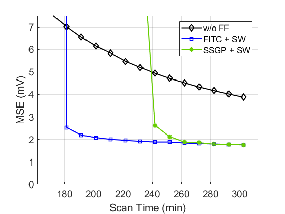
(a)

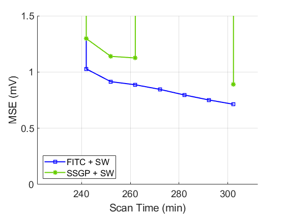
(b)

Figure 12: MSE for scanning R2 at different scan times. w/o FF: ESC only. FITC: Fully Independent Training Conditional. SSGP: Sparse Spectrum Gaussian Process. SW: Sliding Window. (a): $V^{+}$ scan. (b): $V^{-}$ scan.

Now we simulate the scan of a second reference image, denoted as R2 (see [5]), which shows a different surface structure and is about ten times larger than R1.

Regarding the simulation results, both the SoD and the Kronecker approach fail at tracking the reference for the tested scan times. Hence, we omit the corresponding data in Fig. 12.

For the remaining approaches we observe for the $V^{+}$ scan (Fig. 12a) the same behavior as before for R1. For the $V^{-}$ scan (Fig. 12b) however, different observations are made. The ESC without feedforward control fails to track the reference for the tested scan times, which is why we omit showing the corresponding data in Fig. 12b. We further observe that SSGPR has several problems at certain scan times, resulting unreasonably high errors.

Based on the presented simulation results, we can conclude that the FITC has the largest potential for deployment in SQDM control.

V-D Computation Times and Applicability

Figure 13: Average computation time per line in relation to the available time per line (backwards scan time) and the total line scan time. Top: $V^{+}$ scan of R1 at 20 min total image scan time. Bottom: $V^{+}$ scan of R2 at 180 min total image scan time.

As a last step, we investigate the computation times of FITC as it yielded the best results in terms of performance. Exemplarily, in the following we show the results for the $V^{+}$ scans of R1 and R2 (Fig. 13), each with the minimal possible scan time (R1: 20 min, R2: 180 min, see Fig. 11, 12).

We start with the $63\times 63$ pixels image R1. At a total scan time of 20 min, the scan time per line is 19.0 s. As in the experiments and due to the microscope’s software, each line is scanned back and forth. Thus, half of the scan time is for scanning forward (data collection) and half, i.e., 9.5 s, is for scanning backward. The backwards scan time is the time per line that is available for computing hyperparameter learning and inference. For R1, we find this computation time using FITC to be in total 28.1 s. This equals an average computation time per line of 0.45 s. Thus, FITC requires per line only 4.7 % of the available computation time.

For R2 ($200\times 200$ pixels), we find the computation time using FITC to be in total 11.7 min. Following the same argumentation as before for R1, FITC requires only 6.5 % of the available computation time per line.

VI Conclusions and Outlook

For accelerating and improving scanning quantum dot microscopy imaging, a two-degree-of-freedom controller combining Gaussian process regression and extremum seeking control had been proposed. In this work we have developed this control paradigm further to make it suitable to be used for arbitrary surface structures without a priori knowledge. To this end, the crucial steps and therewith the main contributions of this work are, (i) the implementation of an online hyperparameter optimization and, (ii) the approximation of the Gaussian process to reduce computation time.

We have shown that with online hyperparameter adaptation it is now possible to image arbitrary surface structures and found that the fully independent training conditional (FITC) approximation is the best working approach for sparsifying the Gaussian process and to reduce the computational load. The computation time using FITC is sufficiently low for practical applicability.

Future steps will involve the implementation of the proposed approach on the real system and the verification in experiments. Furthermore, future research will be directed to pixelwise predictions by further lowering the computation time or to learn the controller directly instead of separating learning and control as proposed here.

References

- [1] F. Moresco, “Driving molecular machines using the tip of a scanning tunneling microscope,” in Single Molecular Machines and Motors. Springer, 2015, pp. 165–186.
- [2] R. Findeisen, M. A. Grover, C. Wagner, M. Maiworm, R. Temirov, F. S. Tautz, M. V. Salapaka, S. Salapaka, R. D. Braatz, and S. O. R. Moheimani, “Control on a molecular scale: a perspective,” in 2016 American Control Conference, Boston, MA, USA, 2016, pp. 3069 – 3082.
- [3] S. M. Salapaka and S. M. V, “Scanning probe microscopy,” IEEE Control Systems Magazine, vol. 28, no. 2, pp. 65 – 83, 2006.
- [4] C. Wagner, M. F. B. Green, P. Leinen, T. Deilmann, P. Krüger, M. Rohlfing, R. Temirov, and F. S. Tautz, “Scanning quantum dot microscopy,” Physical Review Letters, vol. 115, no. 2, p. 02601, 2015.
- [5] C. Wagner et al., “Quantitative imaging of electric surface potentials with single-atom sensitivity,” Nature Materials, vol. 18, no. 8, pp. 853 – 859, 2019.
- [6] M. Maiworm, C. Wagner, R. Temirov, F. S. Tautz, and R. Findeisen, “Two-degree-of-freedom control combining machine learning and extremum seeking for fast scanning quantum dot microscopy,” in 2018 Annual American Control Conference, Wisconsin Center, Milwaukee, USA, 2018, pp. 4360 – 4366.
- [7] C. Wagner and F. S. Tautz, “The theory of scanning quantum dot microscopy,” Journal of Physics: Condensed Matter, vol. 31, no. 47, p. 475901, 2019.
- [8] M. Krstić, “Performance improvement and limitations in extremum seeking control,” Systems & Control Letters, vol. 39, no. 5, pp. 313–326, 2000.
- [9] J. Quiñonero Candela, C. E. Rasmussen, and C. K. I. Williams, “Approximation methods for Gaussian process regression,” Microsoft Corporation, Tech. Rep., 2007.
- [10] C. E. Rasmussen and C. K. I. Williams, Gaussian Processes for Machine Learning. The MIT Press, 2006.
- [11] J. Kocijan, Modelling and Control of Dynamic Systems Using Gaussian Process Models. Springer International Publishing AG Switzerland, 2016.
- [12] M. Lázaro-Gredilla, J. Quiñonero Candela, C. E. Rasmussen, and A. R. Figueiras-Vidal, “Sparse spectrum Gaussian process regression,” Journal of Machine Learning Research, vol. 11, pp. 1865 – 1881, 2010.
- [13] O. Sigaud and J. Peters, From Motor Learning to Interaction Learning in Robots. Springer-Verlag Berlin Heidelberg, 2010.
- [14] A. J. Smola and B. Schölkopf, “Sparse greedy matrix approximation for machine learning,” in Proceedings of the Seventeenth International Conference on Machine Learning, 2000, pp. 911 – 918.
- [15] M. Seeger, C. K. I. Williams, and N. Lawrence, “Fast forward selection to speed up sparse Gaussian process regression,” in Ninth International Workshop on Artificial Intelligence and Statistics, C. M. Bishop and B. J. Frey, Eds. Society for Artificial Intelligence and Statistics, 2003.
- [16] E. Snelson and Z. Ghahramani, “Sparse Gaussian processes using pseudo-inputs,” in Advances in Neural Information Processing Systems 18, Y. Weiss, B. Schölkopf, and J. Platt, Eds. Cambridge, MA: MIT Press, 2006, pp. 1257 – 1264.
- [17] M. K. Titsias, “Variational learning of inducing variables in sparse Gaussian process regression,” in 12th International Conference on Artificial Intelligence and Statistics, Clearwater Beach, Florida, USA, 2009, pp. 567 – 574.
- [18] A. G. Wilson and H. Nickisch, “Kernel interpolation for scalable structured Gaussian processes (KISS-GP),” in Proceedings of the 32nd International Conference on Machine Learning, Lille, France, 2015, pp. 1775 – 1784.
- [19] K. Chalupka, C. K. I. Williams, and I. Murray, “A framework for evaluating approximation methods for Gaussian process regression,” Journal of Machine Learning Research, vol. 14, pp. 333 – 350, 2013.
- [20] S. Van Vaerenbergh, J. Via, and I. Santamana, “A sliding-window kernel RLS algorithm and its application to nonlinear channel identification,” in 2006 IEEE International Conference on Acoustics, Speech and Signal Processing, vol. 5, Toulouse, France, 2006, pp. 789 – 792.
- [21] W. A. Barbakh, Y. Wu, and C. Fyfe, Non-Standard Parameter Adaptation for Exploratory Data Analysis. Springer-Verlag Berlin Heidelberg, 2009.
- [22] C. E. Rasmussen and H. Nickisch, The GPML Tollbox version 4.2, 2018.
- [23] K.-H. Chang, e-Design. Computer-Aided Engineering Design. Academic Press, 2015.
- [24] I. Avcbas, B. Sankur, and K. Sayood, “Statistical evaluation of image quality measures,” Journal of Electronic Imaging, vol. 11, no. 2, pp. 206 – 223, 2002.
- [25] H. R. Sheikh and A. C. Bovik, “Image information and visual quality,” IEEE Transactions on Image Processing, vol. 15, no. 2, pp. 430 – 444, 2006.