Two-level systems in superconducting quantum devices due to trapped quasiparticles

A major issue for the implementation of large scale superconducting quantum circuits is the interaction with interfacial two-level system defects (TLS) that leads to qubit relaxation and impedes qubit operation in certain frequency ranges that also drift in time. Another major challenge comes from non-equilibrium quasiparticles (QPs) that result in qubit dephasing and relaxation. In this work we show that such QPs can also serve as a source of TLS. Using spectral and temporal mapping of TLS-induced fluctuations in frequency tunable resonators, we identify a subset of the general TLS population that are highly coherent TLS with a low reconfiguration temperature $\sim$ 300 mK, and a non-uniform density of states. These properties can be understood if these TLS are formed by QPs trapped in shallow subgap states formed by spatial fluctutations of the superconducting order parameter $\Delta$. Magnetic field measurements of one such TLS reveals a link to superconductivity. Our results imply that trapped QPs can induce qubit relaxation.

It is becoming increasingly evident that the most coherence limiting TLS reside outside the qubit junctions on the surface of metals and dielectrics surrounding them klimov2018 ; lisenfeld2019 ; burnett2014 ; degraaf2017 ; bilmes2019 and their slowly fluctuating dynamics poses a significant challenge for quantum computation supremacy ; klimov2018 ; lisenfeld2019 ; schlor2019 ; burnett2019 . A wide range of techniques has been developed to study and mitigate such TLS, by developing qubits and resonators into probes of a wider range of material properties schneider2019 ; degraaf2017 ; degraaf2018 ; grabovskij2012 ; lisenfeld2019 ; geaney2019 ; degraaf2015 ; lisenfeld2015 ; lisenfeld2015b . However, charged surface TLS and paramagnetic impurities also result in a stochastic and locally varying backdrop for QPs in the superconductor itself. It is thus important to consider the implications on the ever-present excess number of non-equilibrium QPs in superconducting quantum devices Henrique2019 ; jin2015 ; devoretPRL which must be eliminated in order to increase qubit dephasing times. It is also likely that trapped QPs are responsible for the non-equilibrium relaxation of transmons recently observed devoretPRL . Non-equlibrium QPs can be generated by electromagnetic radiation devisser2012 and from rare high energy cosmic particles impinging the sample, the latter inducing correlated errors in all qubits of a surface code architecture moore2012 .

Here we reveal the implications of a spatially fluctuating $\Delta$ on such QPs. Scanning tunneling spectroscopy studies typically find spatial variations in $\Delta$ of the order of $\delta\Delta=10-20\%$ in moderately disordered superconductors carbillet2019 ; lemarie2013 ; Liao2019 . $\delta\Delta$ gets smaller in very clean superconductors, however, even in exceptionally clean films with negligible intrinsic magnetic disorder an everpresent surface spin density of the order of $\sim 5\cdot 10^{17}$ m^-2 degraaf2017 ; anton2013 ; saveskul2019 results in both flux noise degraaf2017 ; quintana2017 ; anton2013 ; kumar2016 ; paladino2014 ; muller2017 and spatially non-uniform gap suppression saveskul2019 . In thin films the gap is also non-uniformely suppressed by the Altshuler-Aronov effect due to impurity scattering Altshurer_Aronov ; carbillet2019 , as well as thickness variations ivry2014 , particularly relevant for Al aldelta . The clean, low resistance NbN films that we chose to study in this work are characterized by a low carrier density Wong2017 . In such materials it is very likely that the DOS varies significantly, resulting in gap variations.

Crucially, we find that the optimal fluctuation able to trap a QP only has a few bound states. As a result a trapped QP behaves similar to ‘textbook’ TLS, as shown in Fig. 1. We hereafter refer to this type of quasiparticle TLS as ‘qTLS’, which coexist with a large number of conventional glassy TLS. The spatial extent of the gap fluctuation sets the frequency of the qTLS, which means that the density of states (DOS) of these objects is very non-uniform (in contrast to conventional TLS in glasses). We predict a maximum in the qTLS DOS around 6-10 GHz, the frequency range of most qubits (transmons). Relatively shallow traps also imply that even a modest temperature can reshuffle the QPs. We expect the underlying qualitative physics of charge defects formed by trapped QPs to be applicable to most materials, including superconductors in the dirty limit, such as Al used for qubits, but the relevant frequency ranges may differ somewhat due to different material parameters.

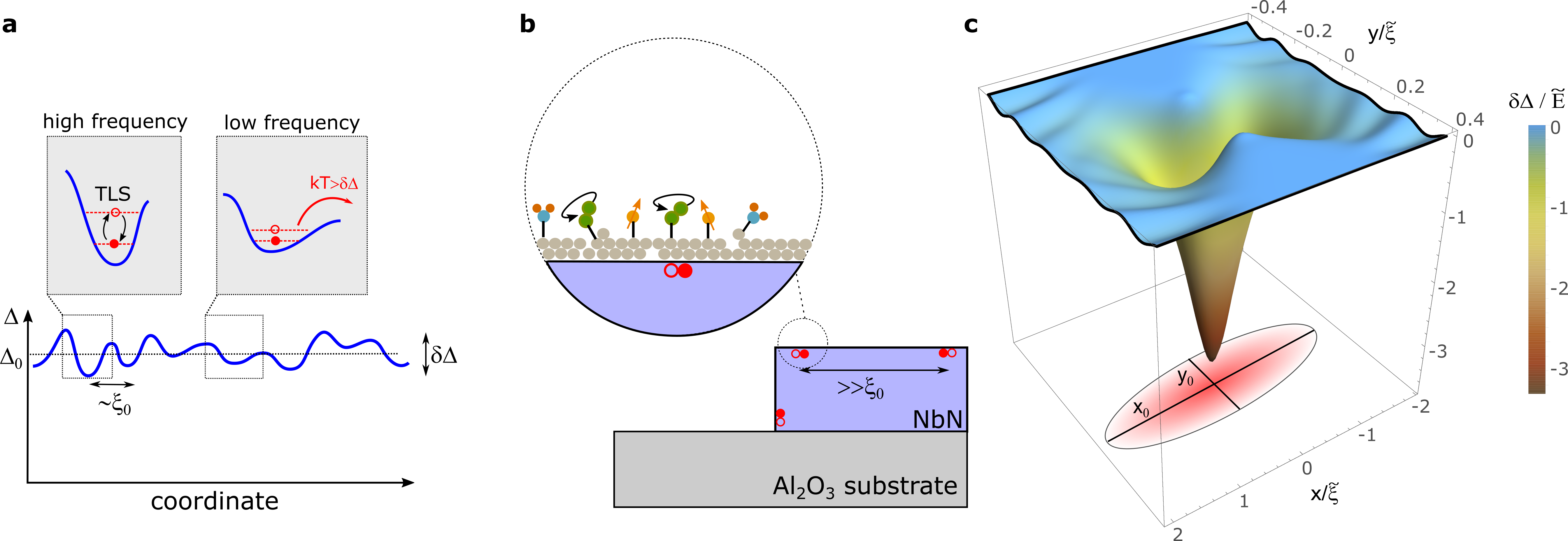
Figure 1: qTLS formation. a) Illustration of typical fluctuations of the order parameter $\Delta$ and the formation of wells with multiple bound states in which quasiparticles can be trapped, effectively forming a TLS (‘qTLS’). The scale of the trap determines the qTLS frequency and escape rate. b) qTLS are separated by large distances compared to length-scales at which fluctuations in $\Delta$ occur, fluctuations which may originate from impurity scattering or surface spins. Importantly the qTLS are separated in distance from the superconductor oxide surface where conventional TLS defects, adsorbants etc. reside, and form the usual bath of TLS. c) Numerically evaluated typical elongated fluctuation of the order parameter capable of hosting multiple bound states for quasiparticles, forming a qTLS. Here $\tilde{\xi}=\sqrt{\Delta_{0}/E}\xi_{0}$, the scaling assumes $(k_{F}\xi_{0})^{-1}=0.14$, $\Delta_{0}/E=40$, appropriate for our NbN samples.

This model is supported by a series of experimental observations from detailed mapping of parameter fluctuations in high-Q frequency tunable superconducting NbN resonators sumedh2019 . Such resonators allow us to map individual TLS in energy and trace them in a broad range of external parameters, such as magnetic or electric field lisenfeld2019 . Through analysis of a large number of individual TLS we find: (i) most qTLS are highly coherent, some with detected linewidths down to $\lesssim 70$ kHz, the resonator linewidth. (ii) The qTLS landscape irreversibly reshuffles at very modest temperatures of $\sim 300$ mK, (iii) The qTLS DOS appears strongly suppressed at lower frequencies. And (iv) tracking a qTLS in magnetic field reveals a qTLS energy that scale in a way similar to the expected scaling of $\Delta$. In particular, the presence of a low energy scale $\lesssim 1\text{K},$ is inconsistent with conventional TLS theory in which all scales are set by chemical energies phillips . The low energy scale is instead natural for TLS formed by QPs trapped in regions of locally smaller gap. We start by outlining the main features of the model that explains these observations.

Results

To understand the emergence of qTLS from a fluctuating $\Delta=\Delta_{0}+\delta\Delta({\bf r})$ we consider a general model that assumes gaussian fluctuations of the gap, $\left\langle\delta\Delta({\bf r})\delta\Delta({\bf r^{\prime}})\right\rangle=g\delta({\bf r}-{\bf r^{\prime}})$, where $g\simeq\delta\Delta\Delta_{0}\xi_{0}^{2}$ is the strength of fluctuations, and $\xi_{0}$ the BCS coherence length. The exact origin of these fluctuations is not relevant for the conclusions. The density of subgap states is determined by rare fluctuations of the gap that reduce the QP energy sufficiently below the gap edge in a uniform material. The key point is that such fluctuations can create traps with a shape and depth that allow them to effectively trap QPs. As the QPs near the gap edge move with momenta close to the Fermi momentum $p_{F}$, it follows that trapped QPs will have similar momenta, which can point in an arbitrary direction. This freedom results in the optimal trap being very anisotropic, with a shape elongated along the direction of $p_{F}$. In Fig. 1c we show the typical shape of such a trap obtained through numerical simulations. In general, the probability to find a fluctuation of depth E scales exponentially with the area $A$ of the fluctuation, $P\sim\exp{(-E^{2}A)}$. Efficient traps thus have small area, however, a too small dimension along the direction of $p_{F}$ will forbid the formation of a bound state due to the large kinetic energy of the QP. Therefore optimal traps do not favor isotropic fluctuations. The wave function of the QP oscillates quickly along the direction of $p_{F}$. The ground and excited states in the trap differ in the number of oscillations: since the total number of oscillations is large it is not surprising that each trap typically contains more than one bound state.

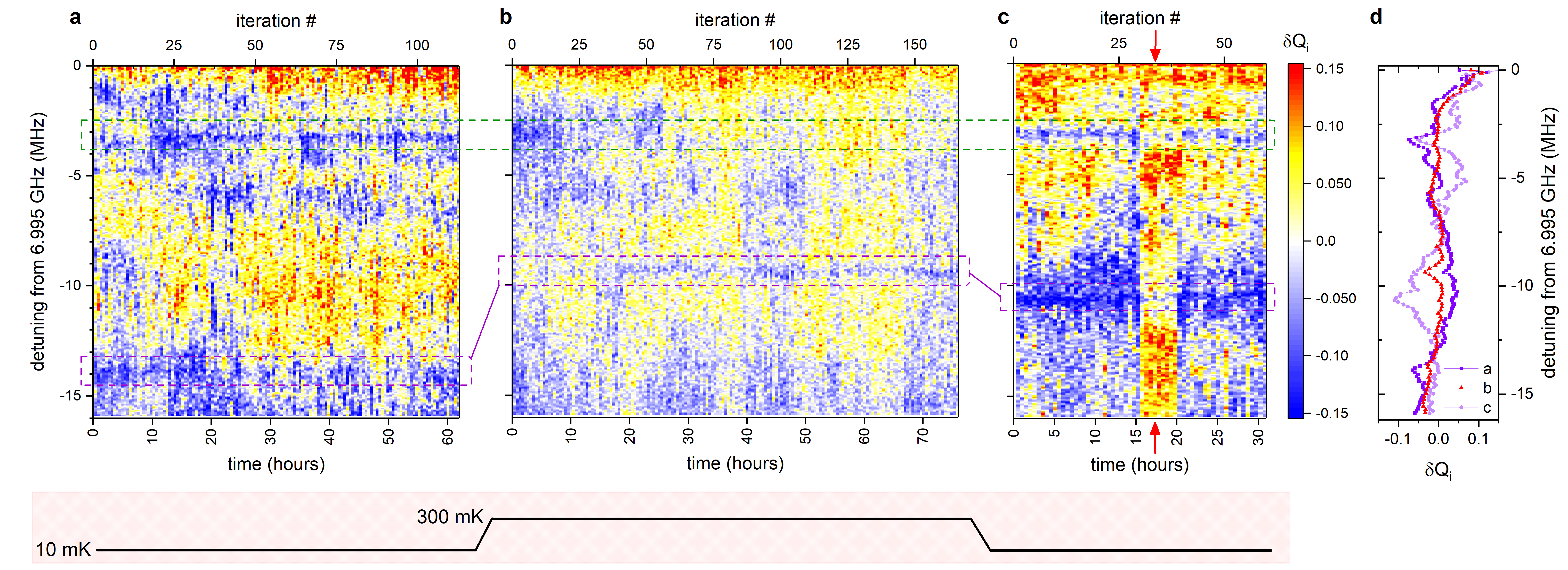
Figure 2: Spectral & temporal fluctuations of the internal quality factor and spectral reconfiguration of TLS. (a) Initial measurement taken at 10 mK and $\langle n\rangle\approx 40$. For each pixel the resonator line-shape is measured and fitted to extract the internal quality factor $Q_{i}$. The measurement is repeated as the resonator is tuned in frequency (the typical frequency resolution is $\approx 50$ kHz), this measurement vs detuning is then repeated over time. The color scale shows the normalised variation $\delta Q_{i}=(Q_{i}-\langle Q_{i}\rangle)/\langle Q_{i}\rangle$. (b) same measurement performed after (a) with the temperature set to 300 mK. (c) the same measurement was repeated again after returning to 10 mK. The red arrows indicate a broad TLS jumping into the measurement window. Dashed boxes indicates two strong TLS. For repeated experiments see suppl . d) The time-averaged data from panels (a)-(c) respectively.

Due to the presence of excited bound states, a QP in such a trap forms an effective TLS with typical energy splitting $\hbar\omega_{\text{qTLS}}=\zeta\left|\widetilde{E}\right|$ where $\widetilde{E}$ is the energy of the trapped QP as measured from the gap edge and $\zeta\approx 0.7$ is found from theory suppl . One consequence of these traps is that, in contrast to conventional TLS, the DOS of qTLS is not constant. A large $\omega_{qTLS}$ implies very deep traps that are exponentially rare. We find the density

$$\rho_{\text{qTLS}}(\omega)\simeq\nu(\widetilde{E})=\frac{1}{\xi_{0}^{2}\Delta_{0}}\text{exp}\left[-\frac{\eta}{g}\frac{\xi_{0}^{2}\Delta_{0}^{2}}{\sqrt{k_{F}\xi_{0}}}\left(\frac{\hbar\omega}{\zeta\Delta_{0}}\right)^{5/4}\right],$$ (1)

where $\eta\approx 10$. Likewise, small $\omega_{qTLS}$ are suppressed since QPs in shallow traps anihilate each other efficiently, leading to

$$\rho_{\text{qTLS}}(\omega)\leq\nu_{0}(\widetilde{E})=\frac{\sqrt{2k_{F}\xi_{0}}}{\xi_{0}^{2}\Delta_{0}[\text{ln}(\tau_{\text{exp}}\Delta_{0}/\hbar)]^{2}}\left({\frac{\hbar\omega}{\zeta\Delta_{0}}}\right)^{3/4},$$ (2)

in the absence of QP generation. Here $\tau_{\text{exp}}$ is an experimental timescale.

Due to the spatial asymmetry, the transition between the lowest and first excited state in each trap is expected to have a significant electric dipole moment, resulting in a strong interaction with quantum devices. In this picture the TLS is formed in a single well, in contrast to the more conventional double-well picture.

In similar films $\delta\Delta$ constitute 10% of the total gap carbillet2019 ; lemarie2013 ; Liao2019 , which gives in our devices $\delta\Delta\approx 2.5$ K. At $T=10$ mK tunneling out of such a local minima is exponentially suppressed, however, at temperatures approaching fractions of $\delta\Delta$ there is a finite probability that the QP escapes and either finds another minima or recombines, resulting in a typical escape temperature of the order of $200-300$ mK; each event resulting in a different TLS landscape.

The unusual shape of the traps and the presence of multiple bound states in each trap distinguish clean superconductors from the dirty limit Larkin_Ovchinnikov ; Lamacraft_Simons ; Silva_Ioffe . In the latter a QP is scattered many times by defects while moving in a particular direction inside the trap, making the formation of elongated traps impossible. The physics of qTLS traps is similar to the well studied phenomena of the appearance of states with negative energy in disordered conductors Halperin_Lax66 ; Cardy1978 , with two important differences: electrons at the bottom of the band in a disordered conductor have much smaller momenta, and the wave functions do not have zeros.

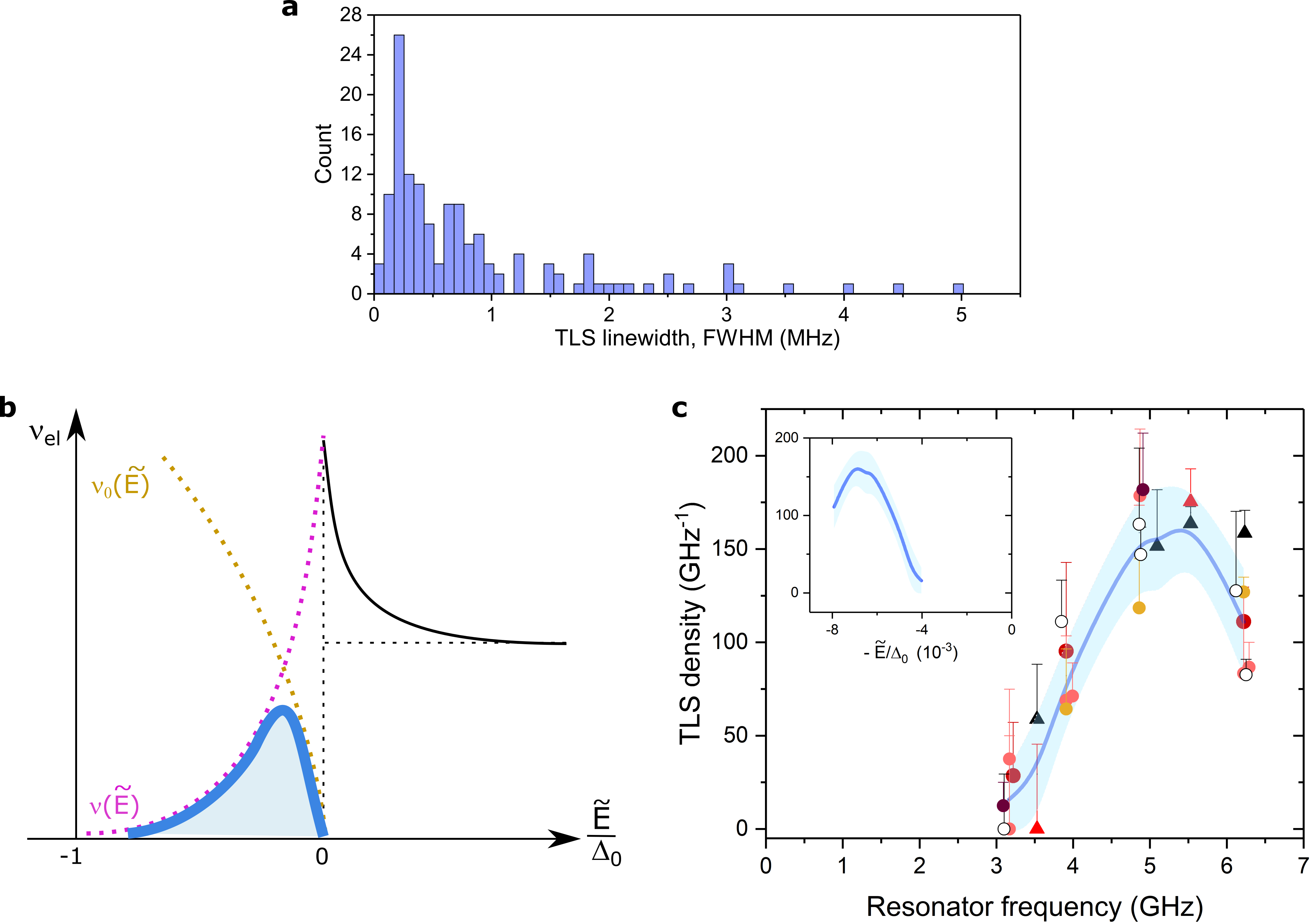
Figure 3: qTLS Properties. a) Histogram of extracted TLS linewidths (FWHM) obtained at 10 mK across a series of cooldowns and different resonators in the frequency range 3-7 GHz. b) Expected scaling of the qTLS density of states (blue solid region) bounded by $\nu(\widetilde{E})$ and $\nu_{0}(\widetilde{E})$ (see text for details). Not to scale. c) Number of strongly coupled TLS as a function of frequency. The data points are obtained by counting the number of TLS present in a spectral and temporal map. Data taken on two different samples (circles and triangles) in seven separate cooldowns (different colors). Duplicate markers at the same frequency are before/after thermal reconfiguration. Multiple markers from the same resonator have been offset somewhat in frequency for better visibility. Error bars indicate miscounting the number of TLS by one, e.g. if one TLS happens to be present just outside the measurement range. The solid line is the average of observations, bounded by the standard deviation. The inset shows the same data plotted against the corresponding trap depth from $\Delta_{0}$. All data obtained at 10 mK and $\langle N\rangle<100$.

We now turn to the experimental work where our observations can be explained by this model. To be able to study individual TLS and spectral and temporal fluctuations of superconducting resonator parameters we use kinetic inductance tunable superconducting resonators with centre frequencies $f_{0}$ in the range 3-7 GHz, described in detail in Ref. sumedh2019 . The resonators are cooled down to a base temperature of 10 mK in a well filtered dilution refrigerator. A small dc current ($<1$ mA) is applied to change the kinetic inductance and tune $f_{0}$. We measure the transmitted microwave signal, $S_{21}$, using a vector network analyser and extract the resonator frequency and quality factors Q. In some of the experiments we also utilise a gate electrode mounted in the lid of the sample enclosure, such that we can affect the TLS energy through the applied gate voltage $V_{g}$: $E_{{\rm TLS}}=\sqrt{\epsilon_{0}^{2}+\gamma^{2}V_{g}^{2}}$ bilmes2019 ; lisenfeld2019 . Here $\epsilon_{0}$ is the TLS minimum energy and $\gamma$ the TLS voltage coupling strength.

In Fig. 2a we show the relative variation of the internal quality factor $\delta Q_{i}=(Q_{i}-\langle Q_{i}\rangle)/\langle Q_{i}\rangle$, as we tune the resonator frequency. The measurement is continously repeated over several days to produce a spectral and temporal map of the variations in loss. This reveals large drops in $\delta Q_{i}$: at detunings of $3.5$ and $14$ MHz (from 6.995 GHz) TLS dips remain in the same place whereas at other frequencies both switching-like behaviour and drift can be observed. We then raise the temperature of the cryostat to 300 mK and repeat the same measurement (Fig. 2b), and return to 10 mK (Fig. 2c). We observe that a strong TLS remains stable over more than 60 hours in each individual measurement, but thermal cycling to a mere 300 mK makes another TLS appear at a different frequency. This is quite remarkable as the temperature is increased to a value smaller than the energy level splitting of the TLS itself (7 GHz $\approx$ 350 mK), and certainly not expected from conventional TLS-glass physics in which all scales are set by chemical energies phillips . Separate high power measurements show that these dips are saturable, and not caused by e.g. local variations in background transmission. We have repeated the same experiment but visiting multiple temperatures on the way to 300 mK (see suppl for additional data) which confirms that reconfiguration only happens near 300 mK.

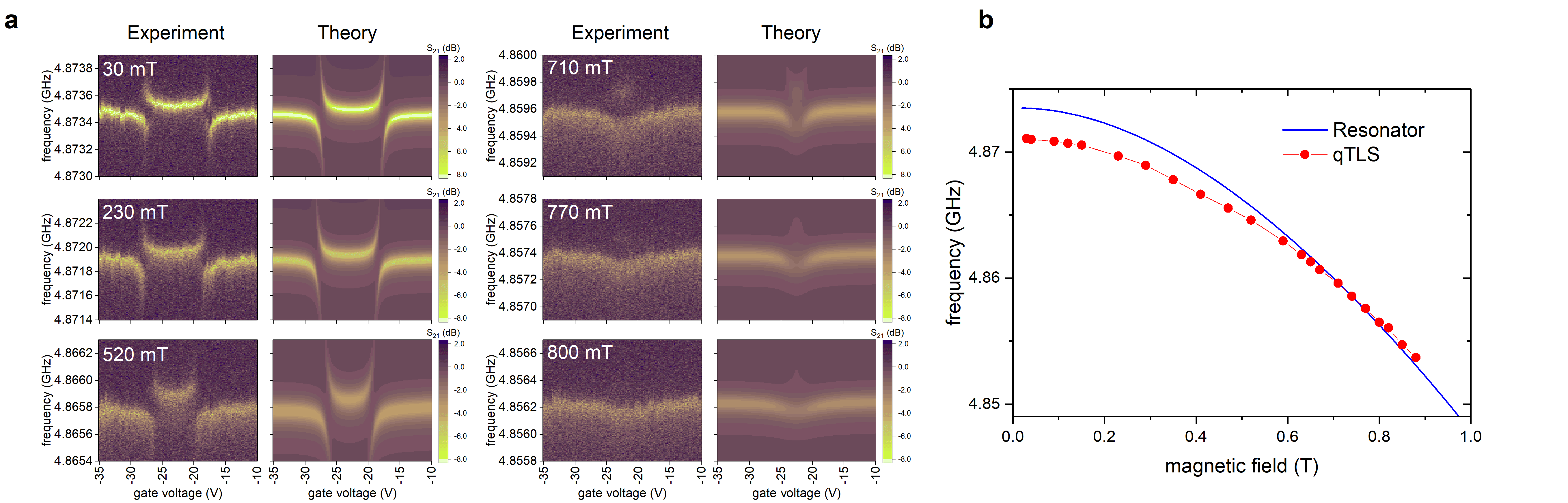
Figure 4: A single strongly coupled qTLS in magnetic field. a) Transmission spectrum of the resonator strongly coupled to a qTLS at selected magnetic fields, as a function of applied electrostatic gate voltage, showing the coherent coupling of a single qTLS to the resonator. b) The resonance frequency as a function of magnetic field (solid blue line) together with the fitted qTLS minimum energy $\epsilon_{0}$ (red markers). Other extracted parameters are qTLS-resonator coupling strength $g_{0}=270$ kHz, damping rate $\gamma_{{\rm qTLS}}=200$ KHz and $\gamma=10$ MHz/V, consistent with $p_{0}\approx 1$ $\rm e\AA$ in our geometry.

Occasionally we observe very dissipative TLS with linewidths in excess of several MHz in our measurement window (red arrow in Fig. 2c). Here we concentrate instead on the much more coherent TLS that we consistently observe, the narrowest with line-widths down to $\sim 70$ kHz suppl , limited by the readout resonator line-width. In Fig. 3a we show the histogram of linewidths of the observed TLS, which peaks at values corresponding to coherence times in excess of several microseconds, much longer than what has been reported for individually resolved TLS in qubits lisenfeld2019 ; lisenfeld2015 . The energy leakage caused by such highly coherent TLS could pose a significant challenge for quantum error correction Brown2019-1 . Naturally, qTLS interact with conventional TLS and slow fluctuators that result in parameter fluctuations.

We now turn to the qTLS DOS. Fig. 3b shows the expected frequency dependence of the qTLS DOS, given by the bounds of eq. (1) and (2). This is in good agreement with the number of strongly coupled qTLS that we observe in resonators with different $f_{0}$, shown in Fig. 3c; data obtained across several cooldowns and devices. A similar dependence was obtained by tuning the TLS energy by an applied electrostatic field, see suppl . In contrast, for conventional non-interacting TLS in amorphous materials we expect a DOS $P(E)={\rm{const}}$ phillips , while for interacting TLS we expect a weak pseudogap given by $P(E)=E^{\mu}$ faoro2015 ; moshe2020 . $\mu\approx 0.2$ is typically found experimentally burnett2014 ; degraaf2018 , which would for $f_{0}=3-6$ GHz only result in a $\sim 10\%$ variation in the TLS DOS. As expected, we find through the temperature dependent shift of $f_{0}$ which samples all TLS, including the more numerous conventional glassy TLS, that the intrinsic loss tangent fall within $F\tan\delta_{i}=0.7\pm 0.1\cdot 10^{-5}$, with no observed dependence on $f_{0}$ suppl .

The data in Fig. 3b has not been scaled to the surface area occupied by each resonator, which would yield an even stronger non-linear dependence ($A\propto f_{0}$). If we make the assumption that the observed qTLS uniformely occupy the surface of the superconductor we get for $f_{0}=4.9$ GHz an observed density of qTLS of $0.004$ GHz^-1 ${\rm\mu}$m^-2, or $1$ GHz^-1 per $(\sim 3000\xi_{0})^{2}$. In our devices the distance between electrodes is small, resulting in significant electric fields away from the immediate vicinity of metal edges. In fact, the maximum observed TLS coupling strengths of up to $100-200$ kHz are obtained for electric dipoles of size $p_{0}\sim 1$ ${\rm e\text{\AA}}$ (the expected scale of a qTLS dipole moment suppl and commonly found also for conventional TLS lisenfeld2019 ; sarabi2016 ) across a significant part of the device surface. Near metal edges we would expect coupling strengths well exceeding 1 MHz suppl . This we do not observe, implying instead that the qTLS are detected across most of the device surface. The above density is much smaller than the total density of TLS we extract from $F\tan\delta_{i}$. We find a surface density of $\rho_{{\rm\Delta,A}}\approx 50$ GHz^-1 ${\rm\mu}$m^-2 of weakly coupled TLS which are mainly responsible for the background loss and noise suppl previously studied in detail burnett2014 ; degraaf2018 . These conventional TLS coexist with the qTLS and constitute the much broader background of loss and fluctuations. However, since the qTLS are located at the metal surface they interact weakly with the conventional glassy TLS bath which is mainly situated some distance away, e.g. in the oxide on the superconductor and adsorbants on top, resulting in higher qTLS coherence.

Finally, to determine if there indeed is a link between the qTLS and superconductivity we measure a strongly coupled qTLS in an applied magnetic field $B$ parallel to the superconducting film, shown in Fig. 4a. As expected, we observe a quadratic suppression of $f_{0}$ owing to the kinetic inductance increasing as $\Delta$ is suppressed. At the same time we track the anti-crossing with the qTLS and extract the minimum qTLS energy $\epsilon_{0}(B)$. As shown in Fig. 4b $\epsilon_{0}$ is also suppressed in magnetic field on a scale comparable to the weak (few %) suppression of $\Delta$. We also note that the conventional TLS bath remains unaffected up to moderate fields degraafAPL2018 .

High-resolution spectral mapping of TLS in qubits has only been performed in the range $5-6$ GHz klimov2018 . Below $3$ GHz qubits in other studies were limited by other loss mechanisms or statistics are insufficient nguyen2019 ; quintana2017 ; yan2015 . Only Ref. quintanathesis hints at a lower TLS density in Al qubits below $\simeq 3$ GHz, suggesting that the mechanism responsible for the formation of qTLS could indeed be quite common, and motivating the need to explore lower frequencies. The critical parameter for the DOS, the strength of fluctuations $g$, is to the best of our knowledge not known for thin Al films. However, it may even be enhanced due to thickness fluctuations contributing to $\delta\Delta$ ivry2014 ; aldelta and the upper frequency for qTLS is bounded by a smaller $\Delta_{0}$. We note that in the dirty limit the details of the theory developed here is not strictly valid. However, the general mechanism would still apply, but the optimal shape of fluctuations is likely to be different.

We now turn to the implications that these qTLS states have for a range of superconducting technologies and for the coherence of qubits. A typical sample of $\sim 1$ cm² size is hit by a high energy cosmic ray once in every $\sim 10$ s, creating a shower of phonons that quickly relax to low frequencies where their relaxation time becomes long. These phonons produce QPs well above $\Delta$. Eventually these QPs fall into the traps discussed here where they remain essentially forever at low temperatures. Such localization of QPs prevents their recombination and equilibration. Those close to a qubit can result in its excitation or relaxation, and hence the QP localization results in a long period of qubit performance degradation. As this degradation affects all qubits on a sample it becomes a catastrophic event for quantum computation, a conclusion supported by recent data on charge noise in qubits mcdermott and by the studies of QP bursts in granular Al resonators Henrique2019 and kinetic inductance detectors karatsu2019 .

Identifying and eliminating strongly coupled TLS is crucially important for scaling-up of superconducting quantum computing. All the mechanisms that lead to gap fluctuations are difficult to control in thin films used for resonators and qubits, but our results suggest these must be carefully addressed in order to achieve this goal.

Supplemental material

Contents

1. A Derivation of the qTLS density of states
2. B Device design and fabrication
3. C Properties of the superconducting film
4. D Measurement setup
5. E Loss tangent
6. F $1/f$ frequency noise
7. G qTLS density in the presence of an electrostatic field
8. H Saturation of individual qTLS
9. I Electron spin resonance spectrum
10. J Thermal reconfiguration of qTLS
11. K Effect of tuning current on qTLS
12. L Surface TLS density
13. M qTLS magnetic field measurements

Appendix A Derivation of the qTLS density of states

Even in very clean superconducting films the gap varies significantly on the scale of superconducting coherence length, $\xi_{0}$. For instance, in ultra clean NbN thin films spatial fluctuations of the order of $\sim 10\%$ in $\Delta$ have been reported in carbillet2019 . These fluctuations can be caused by the inhomogeneous pair breaking by weak magnetic impurities on the surface or by inhomogeneity of the density of states in these films, characterized by very low carrier density. These fluctuations provide traps for quasiparticles with the energies below the average gap, $\Delta_{0}.$ Below we compute the density of quasiparticle states in these traps and their typical spectrum in each trap. We find the a typical trap contains, apart from the ground state, a few localized excited states. We shall assume that gap fluctuations are much smaller than the gap itself, $\delta\Delta\ll\Delta,$ so that the states are formed at energy $\Delta-E$ with $E\ll\Delta$ which is the experimentally relevant case.

Without the loss of generality we can assume that spatial fluctuations in $\Delta$ are described by a white Gaussian noise potential that is characterized by Gaussian statistics with auto-correlation function:

$$\begin{array}[]{c}W({\bf r}-{\bf r^{\prime}})=\langle\delta\Delta({\bf r})\delta\Delta({\bf r^{\prime}})\rangle=g\delta({\bf r}-{\bf r^{\prime}})\\ P(\delta\Delta)=\frac{1}{\sqrt{2\pi g}}e^{-\frac{1}{2g}\int\delta\Delta^{2}dxdy},\end{array}$$ (S1)

where $\delta(r)$ is the dirac delta function. As we show below, the relevant scale for the quasipartcle traps is much larger than $\xi_{0}$, justifying the $\delta$-correlation. We now derive the density of subgap states, $\nu(E)$ and the shape of the optimal fluctuation of the gap that produces them. We focus on the low energy tail. Throughout we use $\hbar=1$. The starting point is the Bogoliubov de Gennes (BdG) equations:

$$\begin{array}[]{c}H_{0}u_{n}({\bf r})+\Delta({\bf r})v_{n}({\bf r})=E_{n}u_{n}({\bf r})\\ -H_{0}v_{n}({\bf r})+\Delta^{*}({\bf r})u_{n}({\bf r})=E_{n}v_{n}({\bf r}),\end{array}$$

where ${\bf r}={\bf\hat{x}}x+{\bf\hat{y}}y$ (we consider the 2D problem, generalization to 3D is straightforward). $H_{0}=\frac{1}{2m}(-i\nabla_{{\bf r}})^{2}-E_{F}$, $E_{F}=\frac{k_{F}^{2}}{2m}$ is the Fermi energy, $\Delta({\bf r})=\Delta_{0}+\delta\Delta({\bf r})$ and $\xi_{0}=\frac{v_{F}}{\Delta_{0}}$ denotes the coherence length of the superconductor. If we regard $u_{n}({\bf r})$ and $v_{n}({\bf r})$ as the upper and lower components of a “spinor” $\psi_{n}({\bf r})$, we can write the effective Hamiltonian acting on this spinor as a matrix: $H=H_{0}\sigma_{z}+\Delta\sigma_{x}$. In the limit $H_{0}\ll\Delta$, we can use perturbation theory to reduce the Hamiltonian $H$ to

$$\widetilde{H}=\Delta+H_{0}\frac{1}{\Delta}H_{0}.$$

The BdG equations then reduce to:

$$\left[\frac{H_{0}^{2}}{\Delta_{0}}+\delta\Delta({\bf r})\right]v_{n}=\widetilde{E}_{n}v_{n}\quad\text{where$\quad\widetilde{E}_{n}=E_{n}-\Delta_{0}<0$ }.$$ (S2)

The BdG equations are valid on the atomic scale and therefore the spinor wave functions $\nu_{n}(r)$, which vary on the length scale set by $k_{F}^{-1},$ contains more information than needed. It is convenient to eliminate these irrelevant degrees of freedom by replacing the BdG equations by their quasiclassical limit. For this purpose one writes the spinor wave function $\nu_{n}({\bf r})$ as a rapidly oscillating phase factor (which changes on the atomic length scale) times a slowly varying amplitude (which changes on a length scale set by the coherence length), i.e. $v_{n}({\bf r})\approx\varphi_{n}(x,y)e^{ik_{F}{\bf\hat{x}\cdot{\bf r}}}$. In this quasiclassical approximation, the quasiparticles are moving along trajectories that are straight lines. We then rewrite the BdG equations neglecting higher derivatives in the $x$ direction

$$\left|\frac{\nabla_{x}^{2}\varphi_{n}(x,y)}{k_{F}{\bf\hat{x}}\nabla_{x}\varphi_{n}(x,y)}\right|\sim\left(k_{F}\xi_{0}\right)^{-1}\ll 1.$$

We find that:

$$H_{0}\approx\left[-iv_{F}\frac{\partial}{\partial x}-\frac{1}{2m}\frac{\partial^{2}}{\partial y^{2}}\right],$$ (S3)

and the BdG equations reduce to:

$$\left\{\frac{1}{\Delta_{0}}\left[-iv_{F}\frac{\partial}{\partial x}-\frac{1}{2m}\frac{\partial^{2}}{\partial y^{2}}\right]^{2}+\delta\Delta({\bf r})\right\}\varphi_{n}(x,y)=\widetilde{E}_{n}\varphi_{n}(x,y).$$ (S4)

After these simplifications, the problem becomes formally similar to the problem of finding the tail in the density of states in disordered conductors Halperin_Lax66 ; Cardy1978 or the density of subgap states due to gap variation in dirty superconductor Larkin_Ovchinnikov . The important difference with these works is, however, the very anisotropic form of the kinetic energy in Larkin_Ovchinnikov .

For the optimal fluctuation all the terms in Eq. S4 are of the same order. This implies that the optimal fluctuation has the size:

$$\begin{array}[]{c}x_{0}=\sqrt{\frac{\Delta_{0}}{\widetilde{E}_{n}}}\xi_{0}\\ y_{0}=\frac{1}{\sqrt{2}\sqrt{k_{F}\xi_{0}}}\sqrt[4]{\frac{\Delta_{0}}{\widetilde{E}_{n}}}\xi_{0}\end{array}$$ (S5)

in $x$ and $y$ directions respectively. Notice that the scales of the two coordinates are different, i.e. $x_{0}\gg y_{0}$, resulting in an optimal gap fluctuation with no spherical symmetry (see Fig. 1c in the main manuscript).

By using Eq. S1, we find that the probability to find the fluctuation $\delta\Delta\sim\tilde{E}$ with spatial extend $x_{0}$ and $y_{0}$ scale as: $\text{ln}P(\tilde{E})=-\frac{\eta^{\prime}}{2\sqrt{2}g}\frac{\xi_{0}^{2}\Delta_{0}^{2}}{\sqrt{k_{F}\xi_{0}}}\left(\frac{\widetilde{E}}{\Delta_{0}}\right)^{5/4}$. For a 3D problem, similar reasoning gives: $\ln P(\widetilde{E})=-\frac{\eta^{\prime}}{2\sqrt{2}g}\frac{\xi_{0}^{2}\Delta_{0}^{2}}{k_{F}\xi_{0}}\frac{\widetilde{E}}{\Delta_{0}}$.

In order to find the exact value of the coefficient $\eta^{\prime}=2\sqrt{2}\eta\sim O(1)$ we need to determine the optimal gap fluctuation that dominates the density of states at energy $\tilde{E}.$ We follow the derivation given in Ref. Halperin_Lax66 of the mian text. By introducing the adimensional coordinates:

$$\begin{array}[]{c}\bar{x}=x_{0}^{-1}x\\ \bar{y}=y_{0}^{-1}y,\end{array}$$

and the scaled wavefunction $\widetilde{\varphi}(\bar{x},\bar{y})=\sqrt{\frac{g}{\widetilde{E}}}\varphi(\bar{x},\bar{y})$, we find that Eq. S4 reads:

$$\left[-i\frac{\partial}{\partial\bar{x}}-\frac{\partial^{2}}{\partial\bar{y}^{2}}\right]^{2}\widetilde{\varphi}(\bar{x},\bar{y})-\widetilde{\varphi}^{3}(\bar{x},\bar{y})-\widetilde{\varphi}(\bar{x},\bar{y})=0,$$ (S6)

and the coefficient:

$$\eta^{\prime}=\int\left|\widetilde{\varphi}(\bar{x},\bar{y})\right|^{4}d\bar{x}d\bar{y}.$$ (S7)

The spectrum operator in Eq. S6 determines the presence (or absence) of excited bound states in the optimal gap fluctuation. Eq. S6 is a fourth order non linear differential equation that we can solve numerically. The solution $\widetilde{\varphi}(\bar{x},\bar{y})$ is illustrated in Fig. 1c in the main manuscript and it represents the optimal trap potential. To solve the non-linear differential equation (S6) we proceed in the following way. The minimization of a generic quadratic functional $F(\phi)$ with the constraint $\Lambda(\phi)$ defined by:

$$F=\int\phi^{*}M\phi dxdy\qquad\Lambda=\int|\phi|^{4}dxdy$$ (S8)

is given by the solution of the Lagrange equation

$$M\phi+\lambda|\phi|^{2}\phi=0$$ (S9)

where $\lambda$ is the Lagrange multiplier. The latter equation can be reduced to equation (S6) by the rescaling of the function $\phi$. Thus, minimizing the functional $F(\phi)$ with appropriate choice of the operator $M$ and rescaling the result we get the solution of equation (S6). The minimization procedure is numerically stable in contrast to the direct solution of the non-linear equation (S6).

The non spherical symmetry is clearly seen and has important consequences for the estimates of the bound states in the typical well. We find that in the optimal trap, beside the ground state $\widetilde{E}$, there is a distintive excited bound state at energy $\widetilde{E}(1-\zeta)$ with $\zeta\approx 0.7$. As a consequence when a quasiparticle is trapped in the optimal gap fluctuation, a qTLS with frequency $\omega_{qTLS}\sim\zeta\left|\widetilde{E}\right|$ can be formed.

As a result of the numerical calculation, we find that the adimensional parameter given in Eq. S7 is $\eta^{\prime}\approx 28$.

Two bound states in the well form the qTLS. We now estimate the density of qTLS, $\rho_{qTLS}(\tilde{E})$. For energies into the low-energy tail, the density of states of the qTLS is given by the electron density of states:

$$\nu(\widetilde{E})\approx\frac{1}{\xi_{0}^{2}\Delta_{0}}\text{exp}\left[-\frac{\eta^{\prime}}{2\sqrt{2}g}\frac{\xi_{0}^{2}\Delta_{0}^{2}}{\sqrt{k_{F}\xi_{0}}}\left(\frac{|\widetilde{E}|}{\Delta_{0}}\right)^{5/4}\right].$$ (S10)

The reason is that at such a low energies, the qTLS are well localized into the optimal gap fluctuations. However, traps with value of energies $\widetilde{E}\to 0$ are very shallow and a trapped quasiparticle can tunnel out of the well and, depending on the time of experiment $\tau_{\text{exp}}$, eventually find a partner and annhilate. If this happens, the qTLS formed in such a shallow trap disappears. We therefore expect that the density of qTLS varies strongly depending on the qTLS frequency. In particular, one would expect that at very high frequencies qTLS are exponentially rare, the majority of qTLS are centered around some typical frequency, and at eneriges corresponding to very shallow traps there are again no qTLS. This is in agreement with what has been observed in the experiment (see Fig. 3c in the main manuscript). We can estimate how the density of qTLS decreases at very small values of $\widetilde{E}$. To this aim, we estimate the tunneling amplitude of the quasiparticle in the trap:

$$t_{\text{amp}}=|\widetilde{E}|\varphi(\bar{x},\bar{y}),$$ (S11)

and expect that two quasiparticles cannot annhilate if

$$\tau_{\text{exp}}t_{\text{amp}}\ll 1.$$ (S12)

Since $\varphi(\bar{x},\bar{y})\sim\text{exp}\left[-\left(\frac{x}{x_{0}}+\frac{y}{y_{0}}\right)\right]$, the condition given in Eq. S12 is satisfied if

$$\frac{x}{x_{0}}+\frac{y}{y_{0}}\gg\text{ln$\left(\tau_{\text{exp}}|\widetilde{E}|\right)$}.$$ (S13)

This translate into the fact that each shallow trap is associated a surface $S=x_{0}y_{0}\text{$\left[\text{ln}\left(\Delta_{0}\tau_{\text{exp}}\right)\right]$}^{2}$ and only for trap densities $\nu_{0}(\widetilde{E})<S^{-1}$, the shallow trap behaves effectively as a qTLS. It is a strightforward calculation to show that:

$$\nu_{0}(\widetilde{E})=\frac{\sqrt{2k_{F}\xi_{0}}}{\xi_{0}^{2}\Delta_{0}[\text{ln}(\tau_{\text{exp}}\Delta_{0})]^{2}}\left({\frac{|\widetilde{E}|}{\Delta_{0}}}\right)^{3/4}.$$ (S14)

As a result one expects that the densities of qTLS at high frequencies decrease as $\rho_{qTLS}<\nu_{0}(\widetilde{E})$. Fig. 3b in the main manuscript shows the theoretical expected density of qTLS.

We also note that the subgap states discussed here are different from Yu-Shiba-Rusinov states due to strong magnetic impurities inside the superconductor. Here each impurity forms a bound state for a QP Fominov2011 , which is related to Kondo physics saveskul2019 ; proslier2008 ; heinrich2017 ; huang2019 . Impurities with Kondo temperature $T_{K}^{*}\sim\Delta$ produce subgap states states in the middle of the gap. Morever, for strong magnetic impurities, energy absorption is due to the tunneling between two subgap states in two different traps. The only energy scale in this problem is $\Delta$, in contrast to our experimental observations.

Finally we make a note on the qTLS electric dipole moment. As the size of the qTLS trap is on the scale $\sim\xi_{0}^{3}$ one would expect a significant dipole moment, however, screening inside the superconductor reduces the effective dipole moment significantly. Any bulk qTLS would have vanishing coupling; only qTLS located at the superconductor surface are expected to couple to external fields. However, even in the most favourable situation when a qTLS trap is located at and oriented parallel to the surface of the superconductor the relevant screening length for perpendicular electric fields is on the atomic scale, $\sim 1$ $\rm\AA$. This sets the scale of the dipole moment for both microwave and electric field induced by the electrostatic gate. The dipole moment we observe both through the coupling to the microwave field and to the DC gate electrode is consistent with this length-scale.

Appendix B Device design and fabrication

The resonator design and fabrication is outlined in detail in sumedh2019 , and the resonators used here are of exactly the same design but of varying length (frequency). The resonator structure is patterned from a 140 nm Nbn film deposited on a heated 2” Sapphire substrate using electron beam lithography. The film is etched in a $Ar:Cl_{2}$ reactive ion plasma which ensures sharp sidewalls and prevents lateral under-resist etching. Wire bonds for rf and dc connections are facilitated by $Au$ bonding pads which are deposited in the next step. The resonator (excluding the ground plane) is thinned down to 50 nm in the same $Ar:Cl_{2}$ reactive ion plasma in the final fabrication step. This yields a sheet kinetic inductance of $\sim 4$ pH/$\square$ and places the resonance frequency in the 3-8 GHz band. The sheet kinetic inductance of the ground plane is lower than the resonator film ensuring that the typical frequencies of the ground plane resonances are placed above 8 GHz. Following the final etching step which produces the final film surface residual resist mask is removed in 1165 remover followed by an isopropanol and water rinse. The final step is a soft $O_{2}$ plasma clean. A second set of samples used to compare the TLS density ustilises a thinner film, 17 nm, with no apparent effect on the qTLS density.

Appendix C Properties of the superconducting film

Figure CS1 shows the resistivity of the film versus temperature for a typical NbN film deposited in our sputtering system. We find a sheet resistance of $R_{\square}\approx 35\Omega$ for a 50 nm thick film and the critical temperature is $T_{c}=14.2$ K and the transition is sharp with $\Delta T_{c}\approx 0.1$ K. The low sheet resistivity and the weak temperature dependence of the resistivity above $T_{c}$ indicates a relatively clean film.

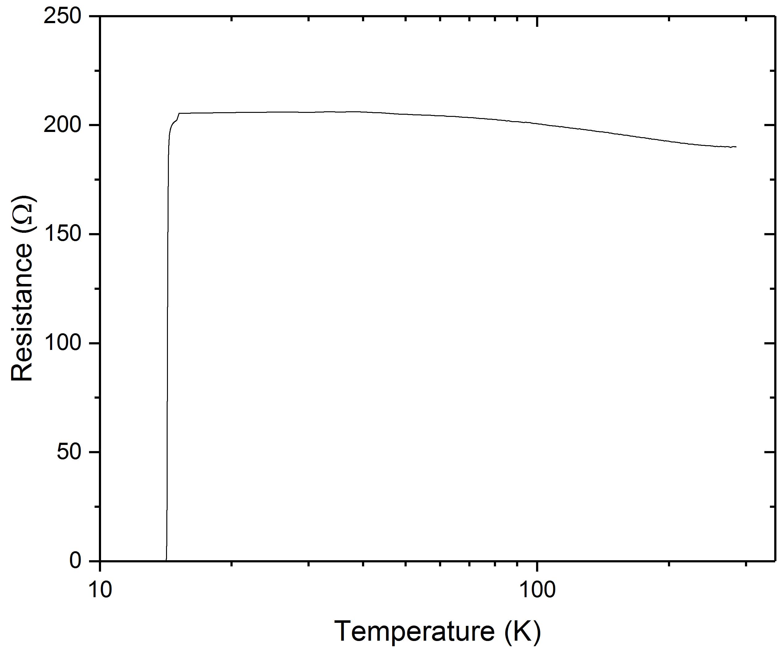
Figure CS1: Resistance versus temperature measured on a 50 nm thick and 6 squares long wire of the NbN film.

Appendix D Measurement setup

Our typical measurement setup is depicted in Fig. DS2. The current that is used to tune the resonator frequency is generated by a voltage source (waveform generator) and converted to a bias current through a 5 k$\Omega$ resistor. The current is fed to the sample through un-attenuated low-pass filtered coaxial lines and back to the 4 K stage of the fridge where it is dissipated in an attenuator terminated with a 50 $\Omega$ load. At 10 mK all the measurement and control lines are typically filtered through home-made eccosorb filters and commercial band- & low- pass filters as appropriate. We note that in some experiments (in particular those in the bore of the magnet) for technical reasons we did not use as elaborate filtering and sample shielding, however, this appears to have no significant impact on the device perofrmance or the TLS observed. During magnetic field measurements the cryogenic isolators on the microwave readout line were also thermalised on the 800 mK stage to avoid significant stray fields from the magnet, at the expense of poorer readout constrast due to an increased amount of thermal photons.

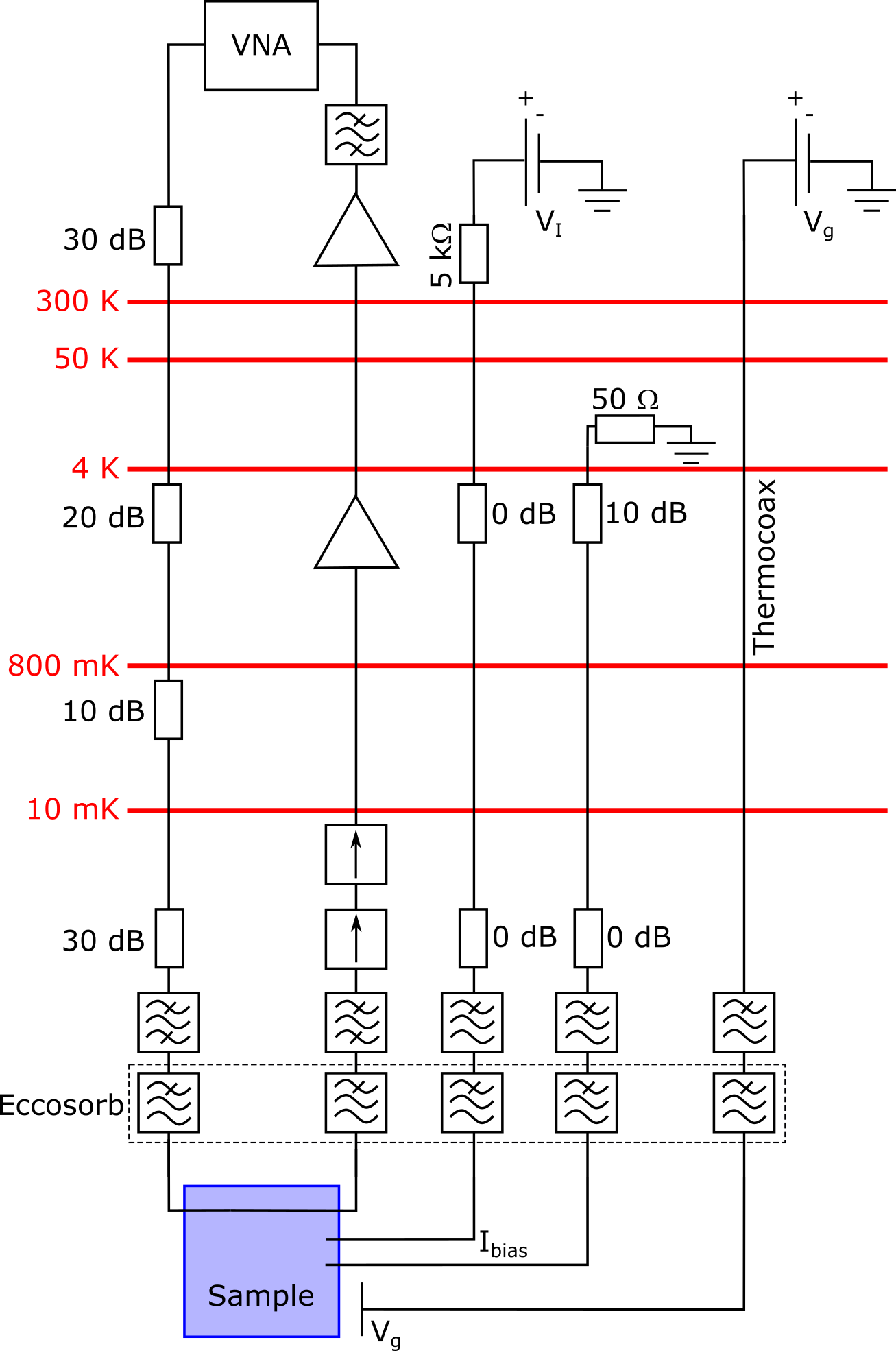
Figure DS2: Schematic showing the main components of the experimental setup.

Appendix E Loss tangent

We next verify the background loss in our resonators, originating from a large ensemble of weakly coupled TLS (the expected usual dielectric TLS material defects in addition to qTLS), by measuring the intrinsic dielectric loss tangent. The intrinsic loss tangent $F\tan\delta_{i}$ (at zero frequency detuning) of each resonator was determined on multiple cooldowns by sweeping the temperature of the cryostat and measuring the resonance frequency versus temperature using a VNA. The intrinsic loss tangent is given by

$$\frac{\delta f_{0}(T)}{f_{0}} = F\tan\delta_{i}\bigg{[}{\rm Re}\bigg{(}\Psi(\frac{1}{2}+\frac{f_{0}h}{2\pi ik_{B}T})+\Psi(\frac{1}{2}+\frac{f_{0}h}{2\pi ik_{B}T_{0}})-\ln\frac{T}{T_{0}}\bigg{)}\bigg{]}.$$ (S15)

Here $\delta f_{0}(T)=f_{0}-f(T)$, $\Psi$ is the di-gamma function, $F$ is a geometric filling factor and $T_{0}$ is a reference temperature. The measured data and fits to Eq. (S15) are shown in Fig. ES3a. For all resonators we find $F\tan\delta_{i}=0.7\pm 0.1\cdot 10^{-5}$, with no clear frequency dependence or variation between cool-downs (verified in three cool-downs). The fitted loss tangents are plotted in Fig. ES3b together with the expected scaling for a constant DOS ($\mu=0$) and a DOS with TLS interactions ($\mu=0.2$). The scatter of the data is within the expected weak dependence of the DOS on resonator frequency.

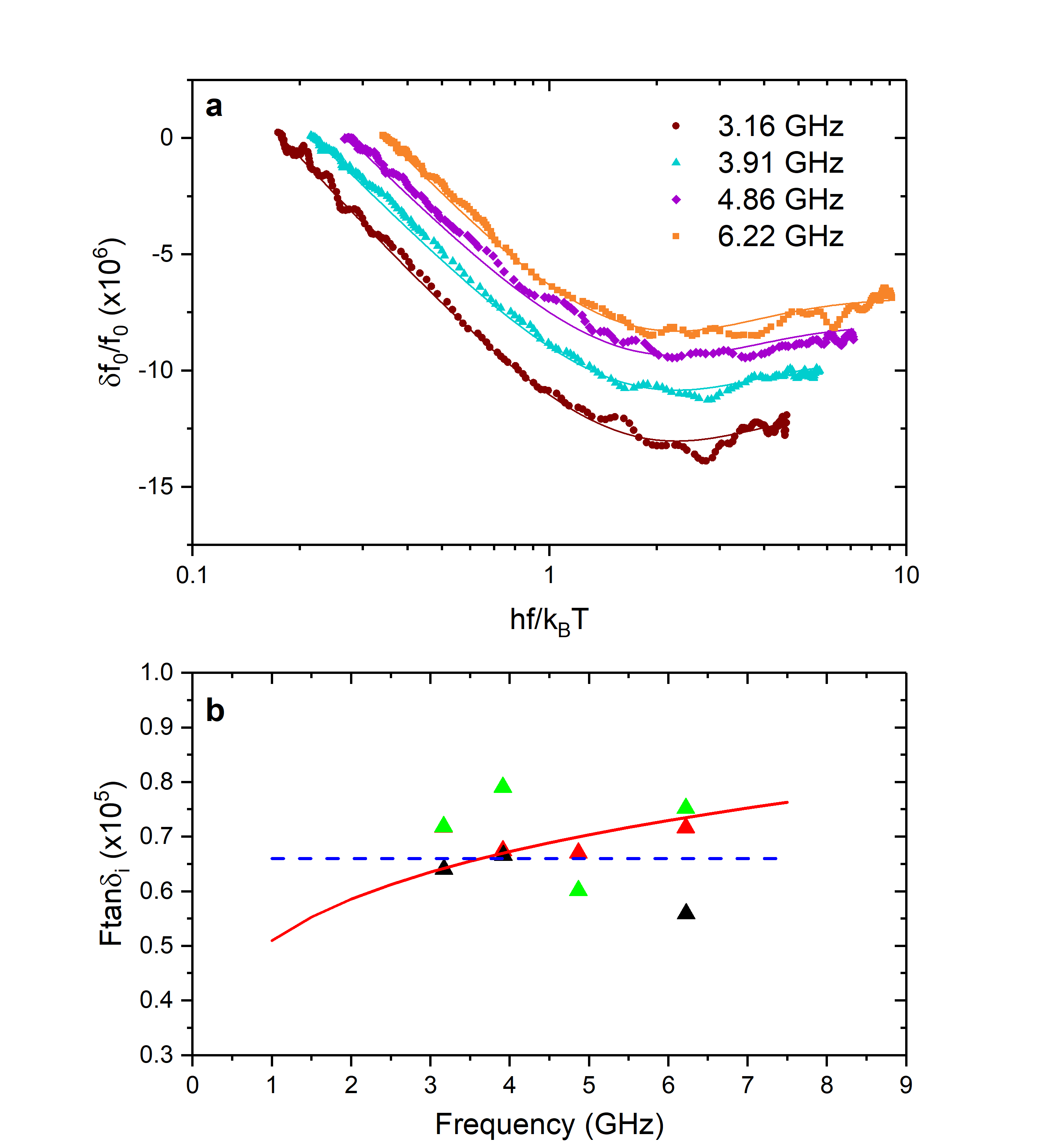
Figure ES3: a) Temperature dependent frequency shift of four resonators measured simultaneously upon cooling down the sample. Solid lines are fits to eq. (S15a) for one measurement cooldown. b) The fitted loss tangents across three cooldowns (different colours) toghether with the expected scaling due to interacting TLS (solid red line, $\mu=0.2$) and the standard tunneling model result (dashed blue line, $\mu=0$), see text for details. Error bars from fits are smaller than the symbols.

Appendix F $1/f$ frequency noise

We also measure the frequency noise of the resonator to ensure that the tuning capability does not induce additional frequency noise. We do this using our Pound frequency locked loop setup described in detail elsewhere tobiaspound ; degraaf2018 . We observe clear $1/f$ frequency noise for the KI tunable resonators of similar magnitude as observed for other resonators of similar capacitor size burnett2016 ; degraaf2018 ; degraafAPL2018 . We measure the frequency noise for a range of powers down to the single photon regime and extract the magnitude of the TLS induced $1/f$ frequency noise, $A_{0}$, by fitting the individual measurements in power to burnett2016

$$S_{y}(f)=\frac{A_{0}}{f\sqrt{1+\langle N\rangle/N_{c}}}.$$ (S16)

Again we find similar values for $A_{0}$ as in previous studies. We then repeat this measurement as a function of resonator frequency detuning and plot $A_{0}(\delta f_{0})$ in Fig. FS4. Indeed, the magnitude of the noise remains unaffected once the resonator is detuned from its base frequency, indicating that the kinetic inductance tuning does not affect the resonator properties in any noticeable way. I.e. no additional kinetic indictance noise nor current noise in the biasing circuitry is large enough to dominate over the intrinsic TLS-induced $1/f$ noise. The larger error bars found for certain detunings are due to strongly coupled TLS causing switching events and the noise deviates from the $1/f$-dependence of the background TLS, and the extraction of the $1/f$ noise level becomes challenging.

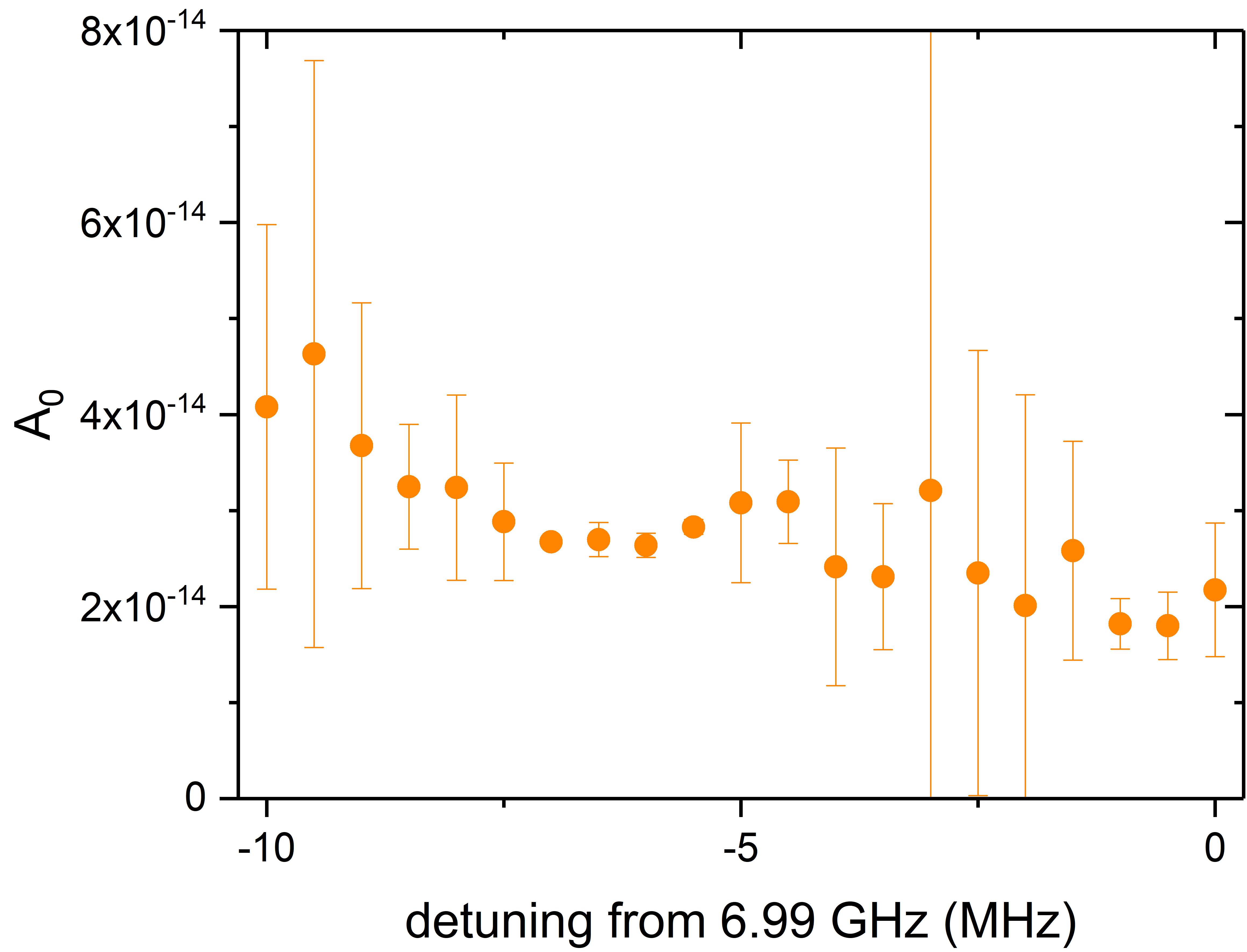
Figure FS4: The magnitude $A_{0}$ of the $1/f$ frequency noise obtained from the power dependence of the measured noise spectral density. Error bars are the standard deviation of the calculated Allan Deviation (ADEV) evaluated across timescales spanning two decades and propagated into the fit to eq. (S16). A small error means that the data is perfectly described by a $1/f$ power law whereas a large error indicates a different noise process coming into play, e.g. a Lorentzian fluctuator. All data obtained at 15 mK.

Appendix G qTLS density in the presence of an electrostatic field

We have also used a complementary technique to extract the qTLS density, by instead tuning the qTLS energies by an electrostatic gate. A gate voltage $V_{g}$ is applied to an electrode located in the sample enclosure, and separated about $z_{0}=2.6$ mm from the surface of the sample. The sample ground planes and resonator structures, PCB on which it is mounted, and the sample enclosure form the counter electrode (ground), similar to the setup in bilmes2019 . The electric field $E\sim V_{g}/z_{0}$ generated at the sample surface couple to the TLS through their dipole moment $p_{0}=qd_{0}$ and its projection angle $\theta$ along the direction of the electric field, such that the TLS energy can be effectively described by $E_{{\rm TLS}}=\sqrt{\epsilon_{0}^{2}+\gamma^{2}V_{g}^{2}}$, where $\gamma=p_{0}\sin\theta/z_{0}$, tracing out a hyperbola as a function of applied electric field. The static electric field distribution is expected to be the same for all resonators. Fig. GS5a shows a typical trace obtained when sweeping the applied gate voltage, here with the background loss subtracted, revealing several qTLS coming into resonance with the resonator. The data was obtained by keeping the resonator at zero frequency detuning, and recording $Q_{i}$ as a function of $V_{g}$. Fig. GS5b shows the number of qTLS found for different resonators when applying a gate voltage. Again, here we see a clear trend with much lower densities of qTLS at low frequencies. Similarly to Fig. 3c in the main manuscript, we have here not taken into account the additional scaling expected from the physical footprint of the resonators, which would require an assumption about the exact locations of the qTLS.

In Fig. GS6 we also show an example of a spectral map from a 3.9 GHz resonator. It is clear that at this frequency the number of TLS observed is much smaller, as compared to e.g. Fig. JS10 below.

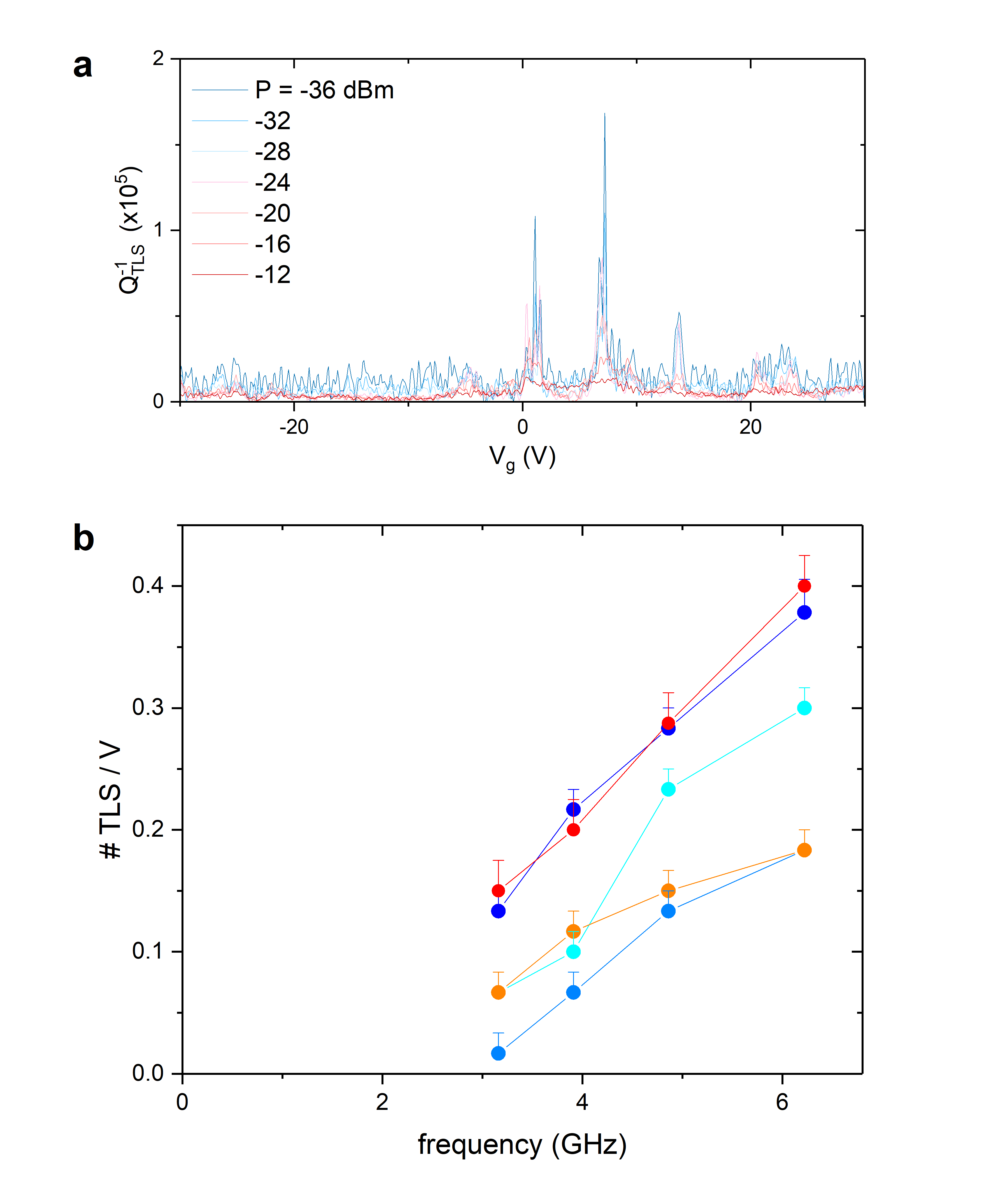
Figure GS5: a) Measured loss rate of individual qTLS brought into resonance with the resonator by an applied electric field ($V_{g}$). Each trace corresponds to a different measurement power, in increments of 4 dB. Here $f_{0}=3.16GHz$. The peaks are due to individual TLS coming into resonance with the resonator. b) Number of strongly coupled TLS as a function of frequency. The data points are obtained by counting the number of qTLS observed as a voltage is applied to a gate electrode located above the sample, tuning the TLS energy by electric field. Multiple data points for each resonator corresponds to separate cool-downs (different color). All data obtained at 15 mK and $\langle N\rangle<100$. Variations in numbers between cool-downs is most likely due to the random distribution of qTLS and the limited range of fields explored. Error bars indicate miscounting the number of qTLS by one, e.g. one is situated just ourside the measurement window.

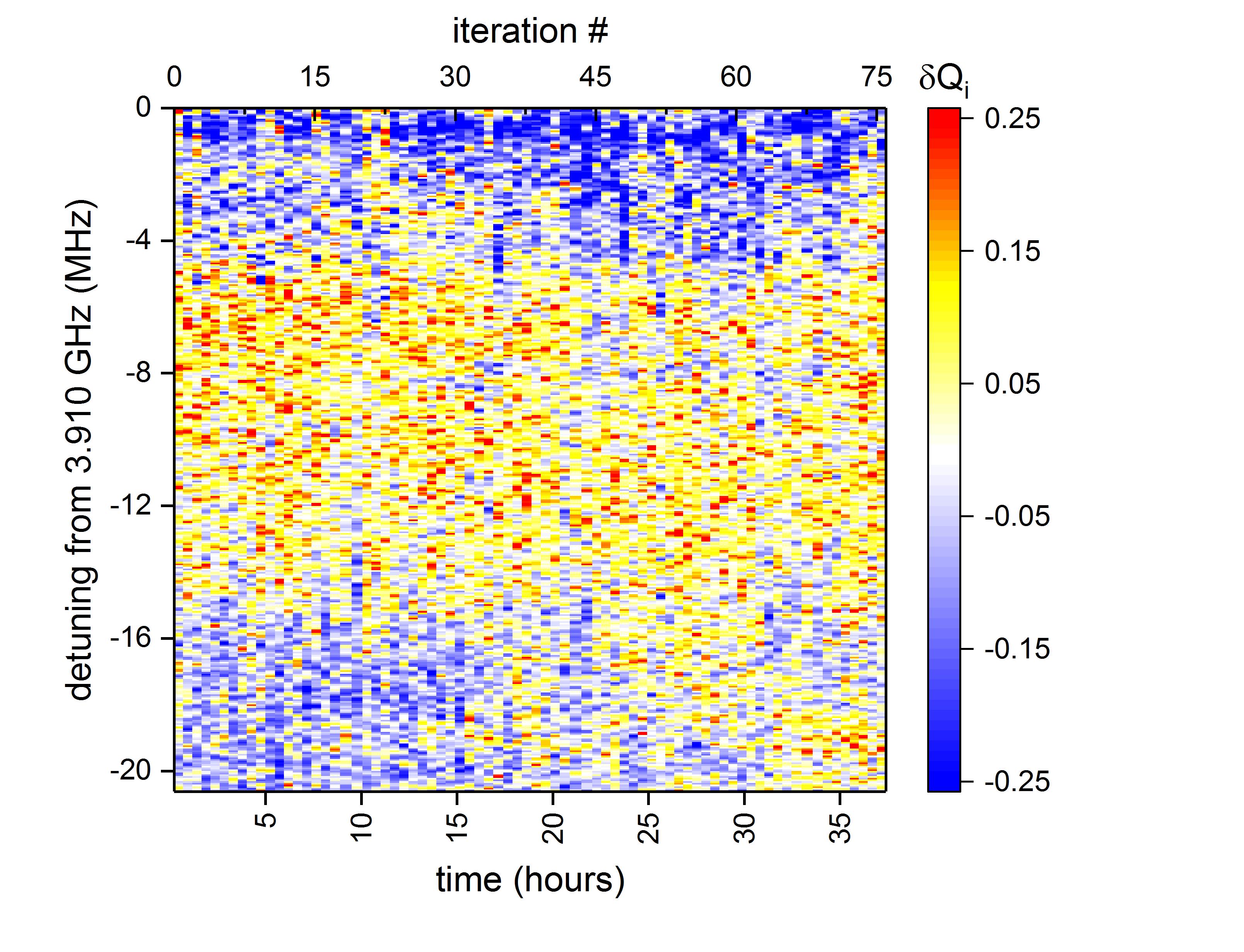
Figure GS6: Spectral & temporal fluctuations of the internal quality factor at 10 mK of a low frequency resonator. $\langle n\rangle\approx 10$. The color scale shows the variation in $Q_{i}$: $\delta Q_{i}=(Q_{i}-\langle Q_{i}\rangle)/\langle Q_{i}\rangle$, where the average is taken across the whole measured parameter space. The detuning is evaluated as the average fitted centre frequency across all times.

Appendix H Saturation of individual qTLS

We next show the saturation properties which further evidences the TLS nature of the observed fluctuations. Fig. HS7 shows the extracted power dependence for saturating individually observed qTLS. For each qTLS we detect as a function of applied gate voltage, we extract its power dependence. From the measured $Q_{i}(V_{g},P)$ we extract for each power the loss rate induced by each qTLS: $Q_{{\rm TLS}}^{-1}=Q_{i}^{-1}(V_{g})-Q_{i,{\rm max}}^{-1}(V_{g})$. We then fit the $Q_{{\rm TLS}}^{-1}(P)$ data to $Q_{{\rm TLS}}^{-1}(P)=Q_{{\rm TLS,0}}^{-1}P^{{\displaystyle\alpha_{{\rm TLS}}}}$ and plot the loss rate versus the power saturation exponent $\alpha_{{\rm TLS}}$ in Fig. HS7. The correlation between $\alpha_{{\rm TLS}}$ and $Q_{{\rm TLS}}$ is expected from the fact that qTLS with large dipole moments strongly affect the resonator and, at the same time also interact strongly with slow fluctuators. I.e. the more dissipative the TLS, the smaller is $\alpha_{{\rm TLS}}$.

Fig. HS8 also shows the measured temperature dependence of the (low power, unsaturated) loss rate of a single qTLS tuned into resonance using the electrostatic gate. The data fits well to $Q_{{\rm TLS}}^{-1}\propto\tanh{(hf_{0}/2k_{B}T)}$ (we ignore the low power saturation regime), which is the expected temperature dependence of a single two-level system.

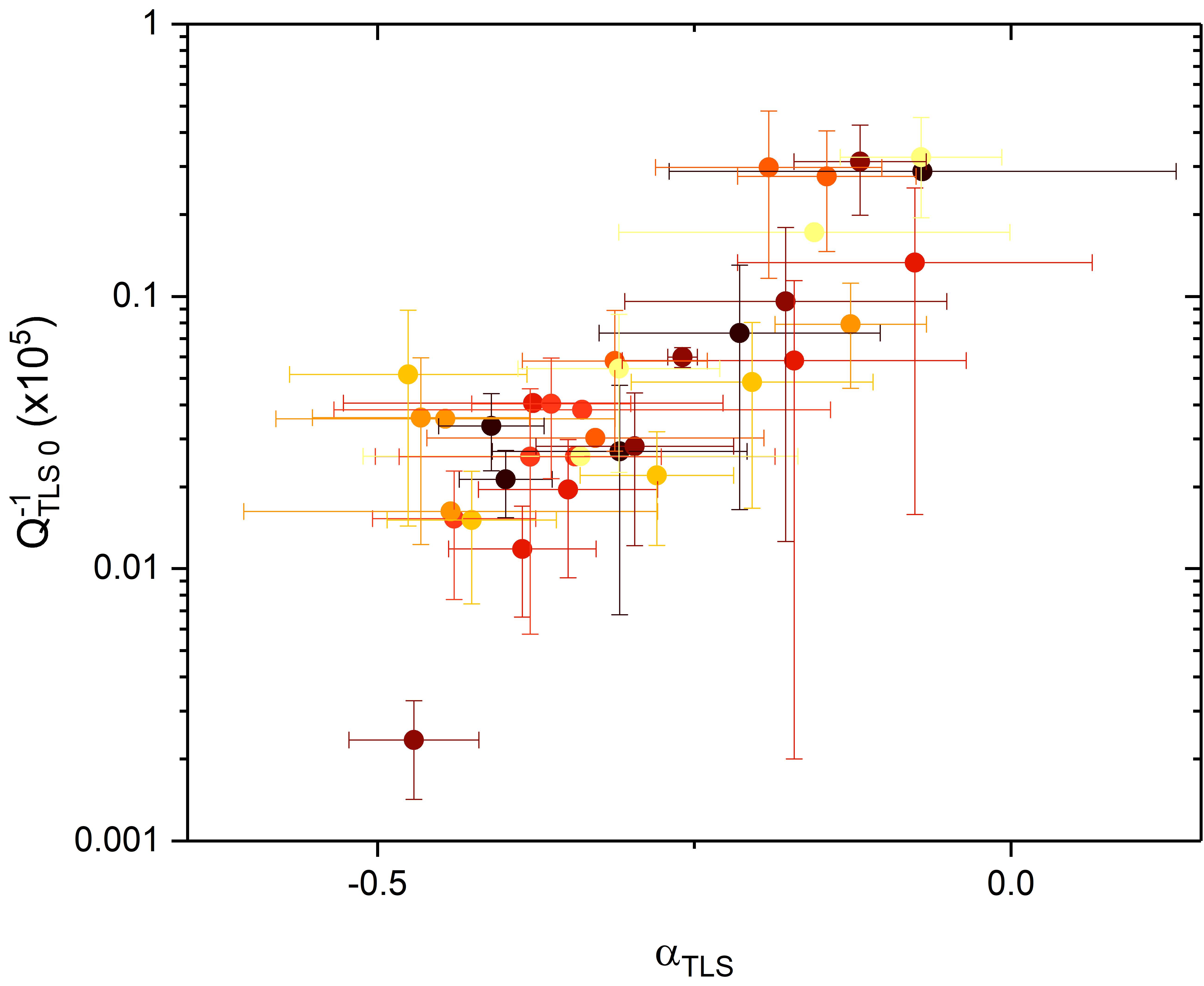
Figure HS7: Loss rate of individual TLS observed through gate tuning, plotted against the power dependence of the TLS. Colors correspond to different resonance frequencies: 6.22 GHz (yellow) through 3.16 GHz (black). Error bars are 95% confidence bounds from the fit to $Q_{{\rm TLS}}^{-1}(P)=Q_{{\rm TLS,0}}^{-1}P^{{\displaystyle\alpha_{{\rm TLS}}}}$. All measurements done at 15 mK.

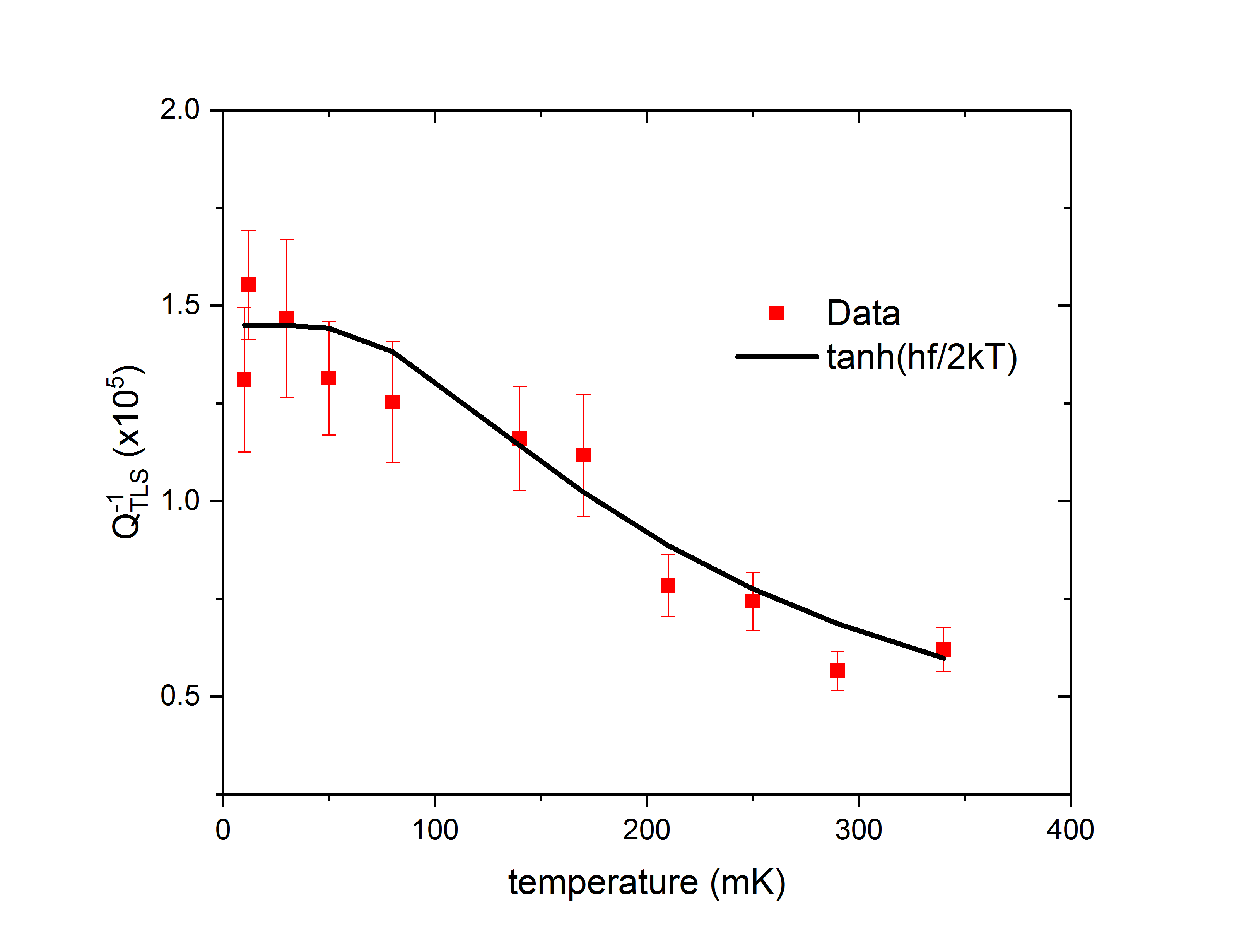
Figure HS8: Temperature dependence of a single qTLS. Each datapoint is obtained by tuning the qTLS through the resonance using an applied gate voltage. The resulting peak in dissipation is then fitted to a Lorentzian with the error bars indicating the 95% confidence bounds. $\langle n\rangle\approx 10$.

Appendix I Electron spin resonance spectrum

Here we show using our constant wave on-chip electron spin resonance (ESR) technique that the samples used here hold the same density and types of surface spins previously analysed in detail degraaf2017 . This amount of surface spins is a likely source of the order parameter fluctuations. The ESR spectrum is shown in fig IS9, where we plot the magnetic field induced loss $1/Q_{i}(B)-1/Q_{i}(B=0)$. While some features can be attributed to certain species degraaf2017 , there is still uncertanity in the broad background plateau starting at about 100 mT, and the nature of the central ’g=2’ peak could, partially, be due to unpaired electrons on the device surface, some of which are likely to be located on the surface of the superconductor. Further measurements will be required to elude any possible ESR signature associated with the qTLS.

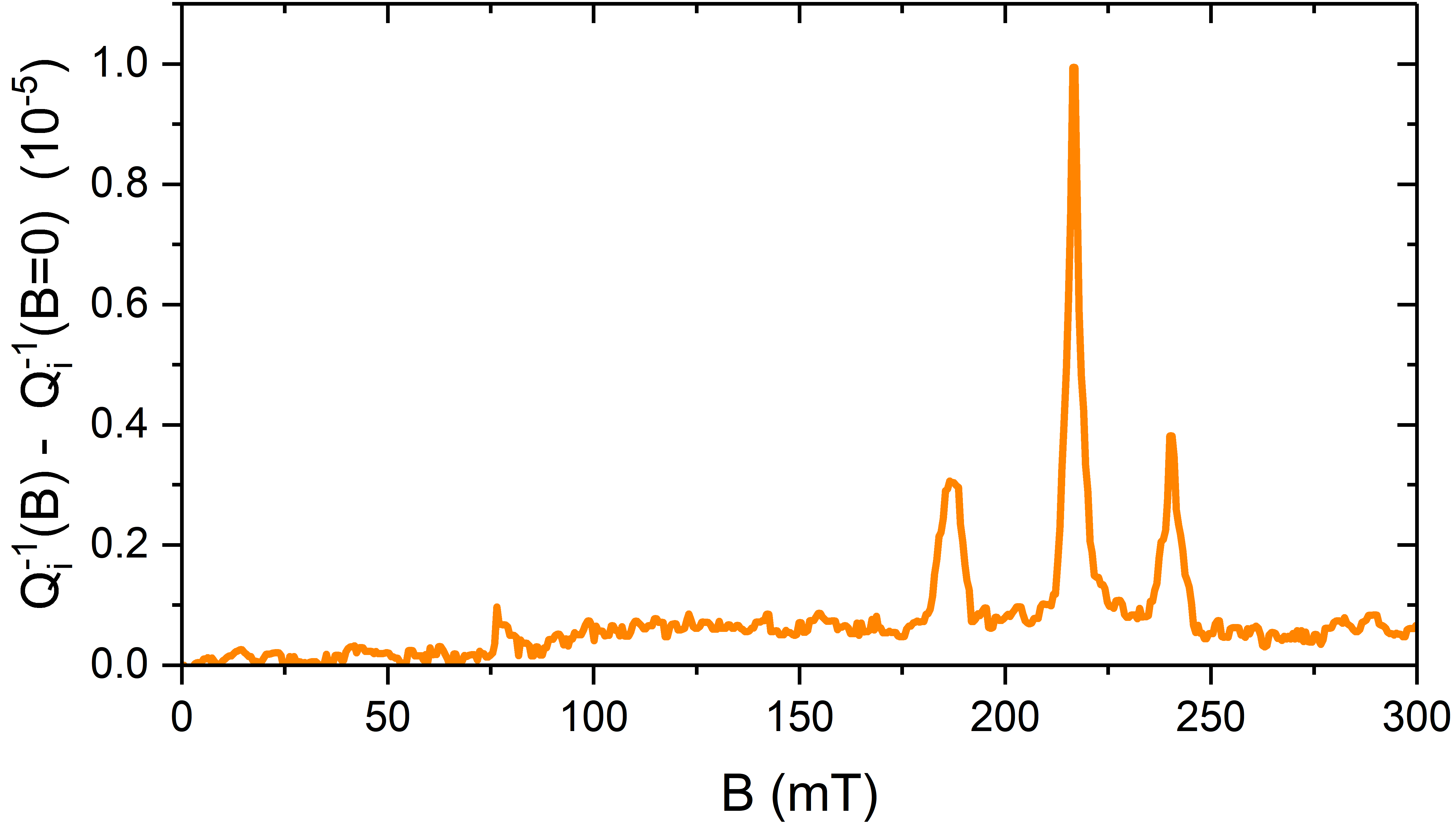
Figure IS9: Intrinsic device on-chip ESR spectrum taken at 10 mK for a 5.87 GHz resonator, showing several features due to surface spins. The plotted quantity is the internal loss rate with the zero field loss rate subtracted.

Appendix J Thermal reconfiguration of qTLS

Here we show additional data from repeated measurements of thermal cycling of the sample, experiments that all indicate a typical energy scale $\sim 300$ mK. Fig. JS10a shows the spectral and temporal dependence of the internal Quality factor of the same resonator that is shown in Fig. 2 in the main manuscript. The data in Fig. JS10a was acquired in a separate cool-down from room temperature, hence a very different TLS configuration. We first perform a measurement at 10 mK, we then raise the temperature to 120 mK for several hours (while acquiring another measurement, data not shown). Returning to 10 mK we record the second set of data. We then repeat this visiting 160, 240, and 320 mK. Again we only see a significant change in the TLS landscape after visiting the highest temperature, 320 mK. The same measurement was repeated for a nother resonator on another sample, and is shown in JS10b. Here, following the gradual increase in temperatures visited we also consecutively visited the highest temperature multiple times, shown in Fig. JS11. This shows moderate stability between thermal cyclings on the timescale of $\sim 24$ hours, after the initial thermal reconfiguration. This would suggest that some qTLS traps where the quasiparticle initially escaped have not been re-populated, but instead different traps are filled due to a non-vanishing flux of new quasiparticles, and these may again be affected by repeated cycling to elevated temperatures. New quasiparticles available for trapping could for instance be generated through high-energy cosmic events or by affecting quasiparticles trapped in different parts of the device.

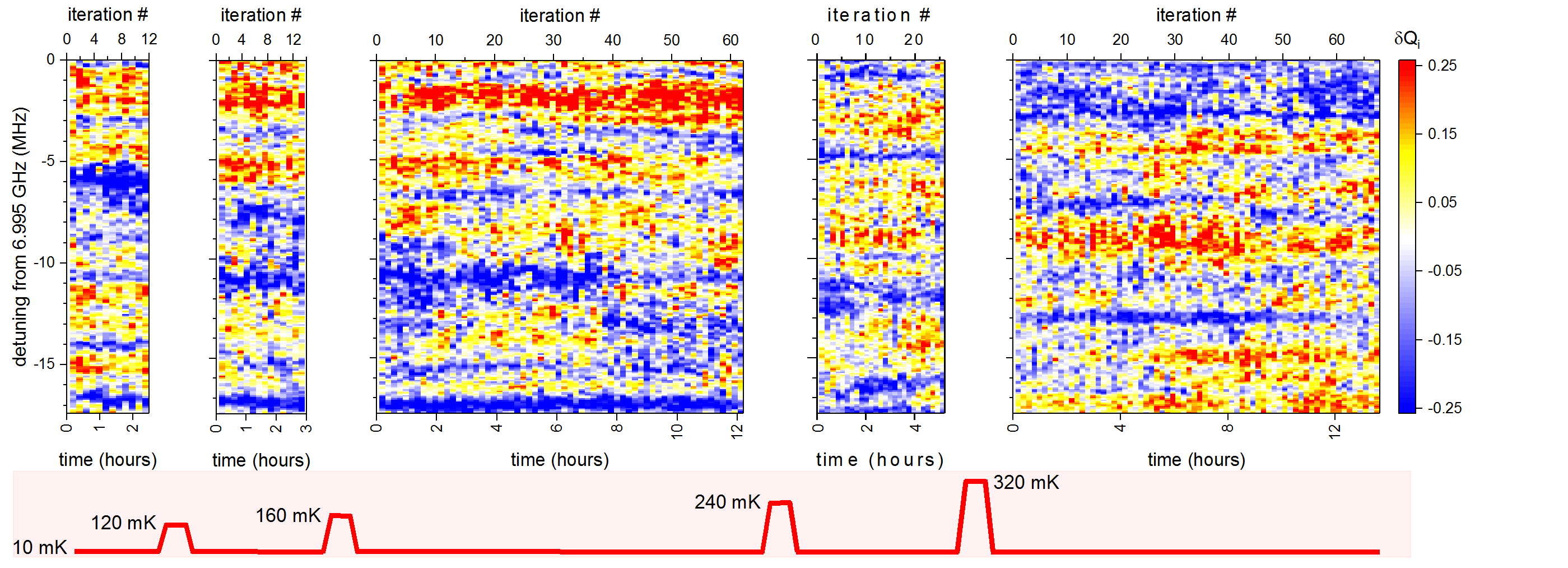
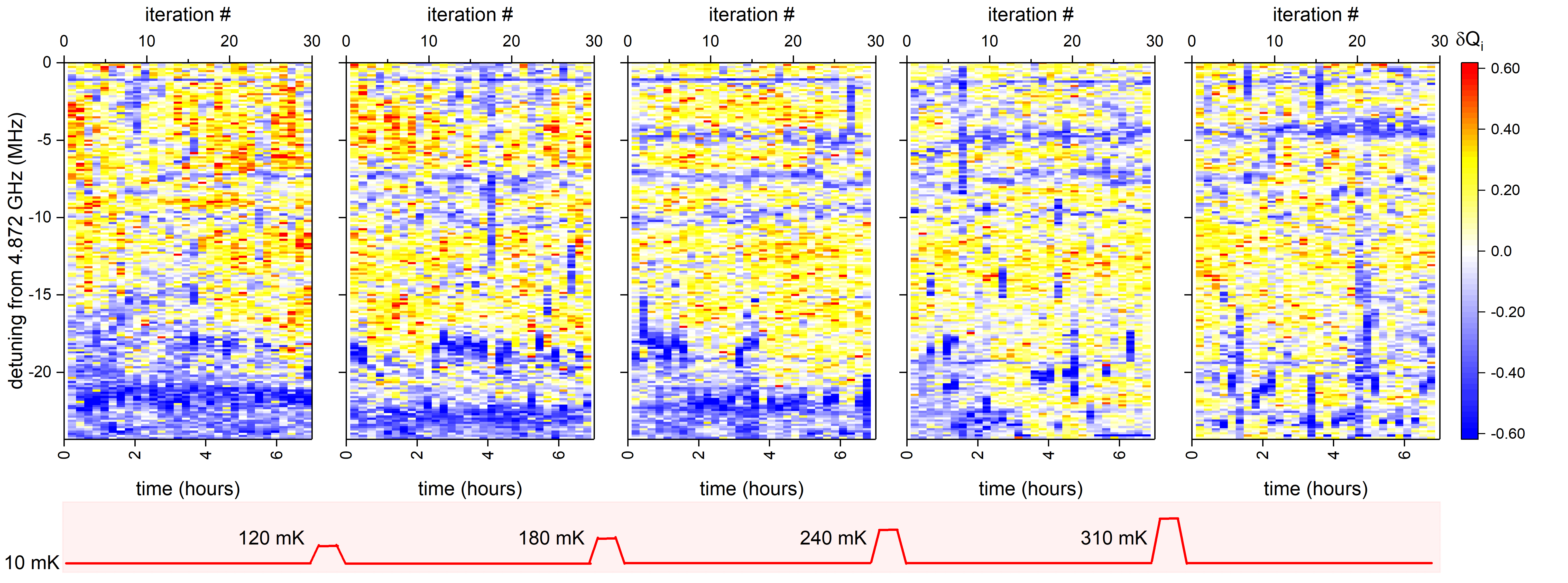
Figure JS10: Thermal reconfiguration of TLS. Spectral & temporal fluctuations of the internal quality factor at 10 mK after consecutive visits to elevated temperatures for two different samples in two different cooldowns. The data in the upper panels is from the same sample but a different cool-down as that in Fig. 2 in the main manuscript. All measurements taken at the same input power to the resonator, corresponding to $\langle n\rangle\approx 10$. The color scale shows the variation in $Q_{i}$: $\delta Q_{i}=(Q_{i}-\langle Q_{i}\rangle)/\langle Q_{i}\rangle$, where the average is taken across the whole measured parameter space. The detuning is evaluated as the average fitted centre frequency across all times.

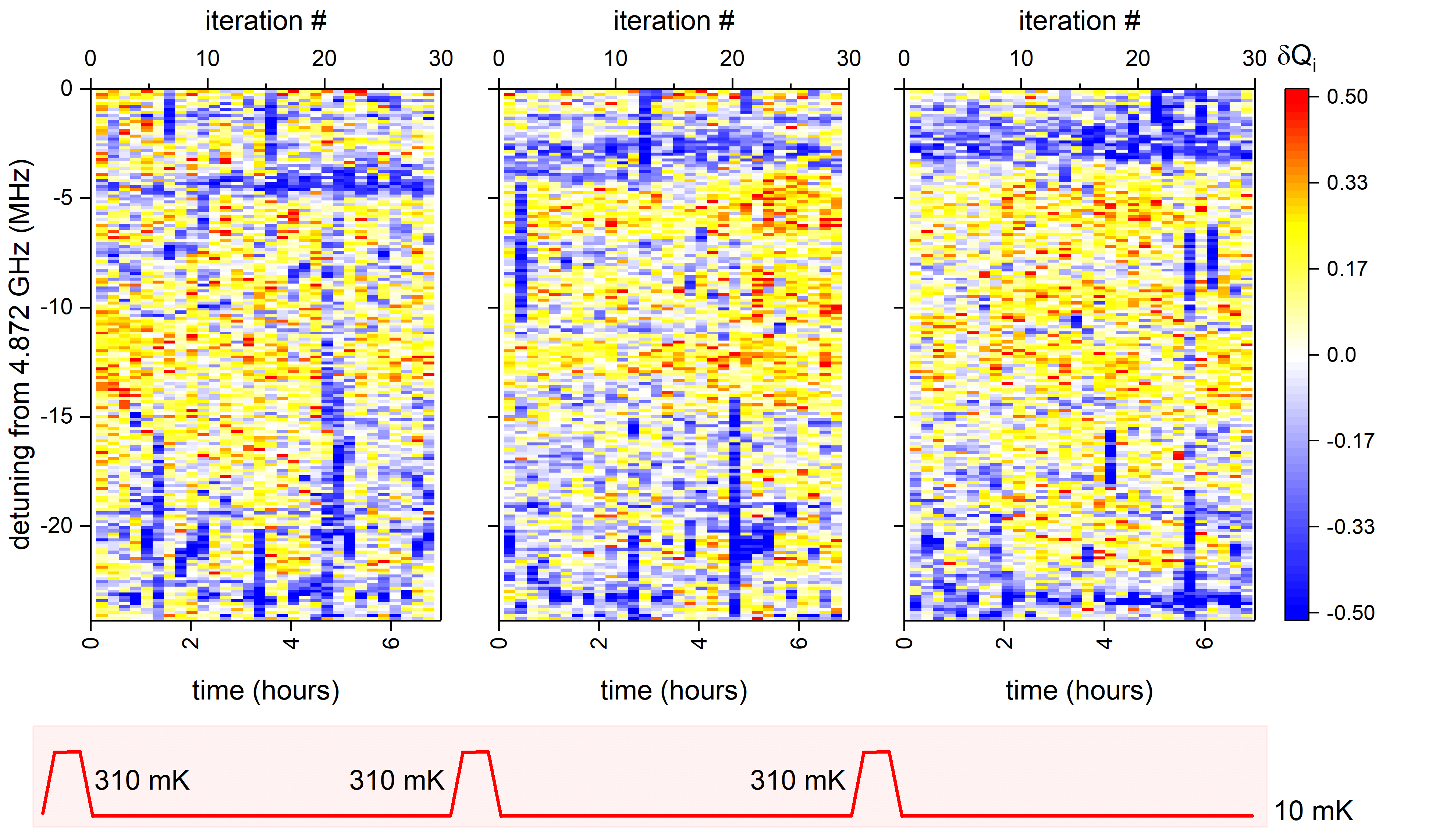
Figure JS11: Thermal reconfiguration of TLS. Spectral & temporal fluctuations of the internal quality factor at 10 mK after repeated visits to 310 mK. All measurements taken at the same input power to the resonator, corresponding to $\langle n\rangle\approx 10$. The color scale shows the variation in $Q_{i}$: $\delta Q_{i}=(Q_{i}-\langle Q_{i}\rangle)/\langle Q_{i}\rangle$, where the average is taken across the whole measured parameter space. The detuning is evaluated as the average fitted centre frequency across all times.

Appendix K Effect of tuning current on qTLS

Another aspect to consider is whether the applied tuning current has any impact on the observed qTLS. In Fig. KS12a we first verify the temporal stability of a few observed qTLS, similar to previous temporal plots shown. After this experiment we immediately start another one (Fig. KS12b) using the same parameters, except after each frequency sweep of the resonator we detune the resonator to a larger and larger frequency (for about 10 seconds), the tuning current approaching the critical current of the superconducting film. Naively one would expect the tuning current to have a similar effect as suppressing the gap, modifying locally the quasiparticle traps. The frequency to which the resonator was detuned is indicated in Fig. KS12c. Notably, we do not observe any major effect on the observed qTLS which could not be attributed to temporal instabilities in this experiment. This is, however, to be expected since superconductivity is only suppressed in the current-carrying parts of the resonator, whereas the qTLS that can be detected are situated in the regions of the resonator with large microwave electric fields, separated large distances from the regions where the DC tuning current flows and the qTLS traps are already occupied. Thus, the shape of the qTLS potentials that couple electrically is never altered, unless the critical current is exceeded and the resulting Joule heating leads to thermal reconfiguration.

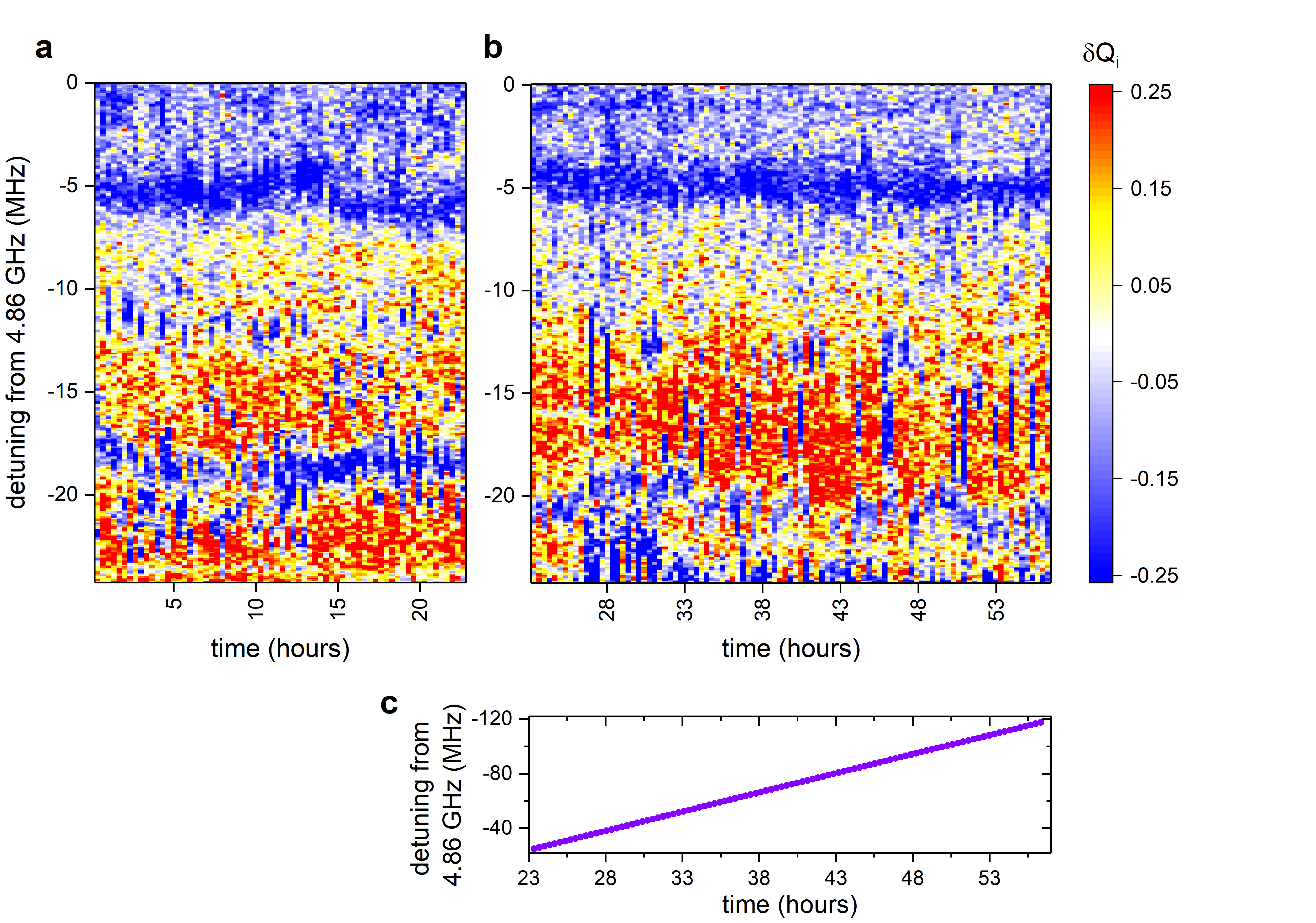
Figure KS12: Effect of a large tuning current on the qTLS. a) Spectral and temporal map of resonator quality factor fluctuations, similar to previous plots presented. The same measurement is simply repeated over and over for 24 hours to verify the temporal stability of observed qTLS. b) Just after the experiment in a) we continue the spectral mapping, but after each measured trace the resonator is detuned for 10 seconds to a higher frequency, as indicated in c), up to near the critical current of the resonator.

Appendix L Surface TLS density

We now turn to the evaluation of the E-field numerical simulations of our device for the evaluation of the conventional background TLS density using several different approaches.

First, following the method in burnett2016 we evaluate the density from the measured loss tangent. Assuming a dipole moment $p_{0}=0.8$ $\rm e\AA$ lisenfeld2019 and a dielectric constant $\varepsilon_{r}=10$ of the TLS hosting medium assumed to be within a surface layer of thickness 10 nm across the whole resonator modal area we find the total number of conventional resonant TLS coupling to the resonator $N_{{\rm TLS}}=\chi\Gamma_{2}V_{r}/U_{0}\approx 430$, where $V_{r}$ denotes the volume occupied by the TLS, $U_{0}=p_{0}^{2}/\varepsilon_{0}\varepsilon_{r}=10^{-2}$ eVnm³, $\chi=F\tan\delta_{i}$ and $\Gamma_{2}\approx 20\chi(k_{B}T)^{1+\mu}/(hf_{0})^{\mu}\approx 7$ MHz at $T=50$ mK, where we have used the Filling factor $F=0.015$ and $\mu=0.2$ burnett2014 . This translates to $\rho_{{\rm TLS}}\approx 60$ GHz^-1 ${\rm\mu}$m^-2, two orders of magnitude larger than the number of observed individual strongly coupled qTLS. This is similar to what is typically found for this type of resonator burnett2016 ; degraaf2018 .

To evaluate the TLS density and contribution to device loss the above and other approaches used so far are almost exclusively reliant on the evaluation of either a participation ratio or filling factor of the dielectric volume of interest. These approaches have two critical disadvantages when delaing with very thin (and often unknown) layers of TLS on surfaces in the form of thin native oxide layers or surface adsorbants. First, an assumption about the layer thickness has to be made, and chosing the correct thickness is not trivial, however, it can have a significant impact on the final result. Furthermore, the dielectric constant of the volume where the TLS are situated is required, and in particular for a monolayer of surface adsorbates this is not very well defined.

Here we instead derive a direct approach to obtaining the TLS density assuming all TLS of relevance reside on a surface. The only quantity that needs to be determined is the electric field strength generated by the device, at the surface of interest, and an assumption of the density of TLS (here assumed to be constant both in energy and spatially). This approach is valid for a distribution of TLS out of the plane of the surface (i.e. thin layers of finite thickness), as long as the electric field strength does not change significantly when the TLS is located outside the evaluated surface.

In the low power limit we can write the total TLS-limited loss as the sum of loss originating from a larger number of TLS.

$$\frac{1}{Q_{{\rm TLS,tot}}}=\sum_{n}\frac{1}{Q_{{\rm n}}}.$$

The absorption of a single TLS is given by its polarisation

$${im}\langle S_{1}^{+}\rangle=\frac{\frac{1}{2}\tanh{\frac{\omega}{2k_{B}T}}\Omega\Gamma_{2}}{(\omega-\varepsilon)^{2}+\Gamma_{2}^{2}+\Omega^{2}\Gamma_{2}/\Gamma_{1}},$$

where $\Omega={\frac{1}{2}{\bf p\cdot E}}/h$ is the Rabi frequency due to the coupling of the TLS dipole to the resonator RF electric field. In the low temperature, low drive regime we thus have

$$\frac{1}{Q_{{\rm TLS,tot}}}=\sum_{n}\frac{{\frac{1}{2}{\bf p_{n}\cdot E_{n}}}\Gamma_{2,n}/h}{\Delta_{n}^{2}+\Gamma_{2,n}^{2}}.$$

First, integrating over all possible detunings (assuming a uniform distribution in frequency of TLS) we get

$$\frac{1}{Q_{{\rm TLS,tot}}}=\frac{\pi}{2h}\rho_{\Delta}\sum_{n}{\bf p_{n}\cdot E_{n}},$$

where $\rho_{\Delta}$ is the energy density of TLS (in number of TLS per Hz). We then assume the ensemble average $p_{0}$ of dipole moments

$$\frac{1}{Q_{{\rm TLS,tot}}}=\frac{\pi p_{0}}{2h}\rho_{\Delta}\sum_{n}{|{\bf E}_{n}||\sin\theta_{n}|},$$

where $\theta_{n}$ is the angle between each TLS dipole and the local electric field. As the RF electric field is perpendicular to the metal surface, the averaging of $\theta$ goes over all possible angles of the TLS orientation only (an approximation that holds for the metal surface but not the substrate-air). The local electric field can be expressed as ${\bf E}=E(x,y)$. We can then convert the sum to an integral over the surface of the superconductor by assuming a uniform surface density (combined with the energy density) $\rho_{{\rm\Delta,A}}$ of TLS

$$\frac{1}{Q_{{\rm TLS,tot}}}=\frac{\pi p_{0}}{2h}\rho_{{\rm\Delta,A}}\int_{A}\int_{0}^{2\pi}E(x,y)|\sin\theta|dxdyd\theta.$$

We can decompose the electric field into a component running along the resonator and one component along the perimeter of the metal. Along the length $L$ of the resonator the field is decaying sinusodially ($\lambda/2$ or $3\lambda/2$ resonator), such that the integrand in $y$ becomes $L/2$.

$$\frac{1}{Q_{{\rm TLS,tot}}}=\frac{\pi p_{0}}{2\sqrt{2}h}\rho_{{\rm\Delta,A}}\frac{L}{2}\int E(x)dx.$$

The remaining integral is carried out in COMSOL by evaluating the electric field around the surface of the superconductor. Details of such simulation for our device is presented in Fig. LS13. For a single photon maximum RF field amplitude of $V_{ph}=\sqrt{4\pi hf_{0}^{2}Z}=3.5$ ${\rm\mu}$V the integral takes in our case the value $\int E(x)dx=2\cdot 10^{-5}$ V around the perimeter of the superconductor (cross-section), including both the M-A and S-M interfaces. Assuming $p_{0}=0.8$ eÅ, we get for $f_{0}=4.9$ GHz

$$\frac{1}{Q_{{\rm TLS,tot}}}=0.003\rho_{{\rm\Delta,A}}.$$

For the measured single photon $Q_{{\rm TLS,tot}}=10^{5}$ we get $\rho_{{\rm\Delta}}\approx 3.4\cdot 10^{6}$ GHz^-1 integrated over the area of the resonator, or $\sim 330$ resonant TLS (within the bandwidth of the resonator). Dividing out the area of the surface of the superconductor in our resonator we find $\rho_{{\rm\Delta,A}}\approx 50$ GHz^-1 ${\rm\mu}$m^-2. These resonant TLS are weakly coupled and each TLS do not contribute significantly to the total loss, for instance these could be the vast majority of TLS with a dipole moment mostly perpendicular to the electric field oriantation.

In the high power limit we instead get

$$\frac{1}{Q_{{\rm TLS,tot}}}=\frac{\pi}{2}\rho_{\Delta}\sum_{n}\frac{\Omega_{n}}{\sqrt{1+\Omega_{n}^{2}/\Gamma_{1,n}\Gamma_{2,n}}},$$

where we can identify a ’critical’ field strength for saturation of the TLS $E_{n,crit}=h\sqrt{\Gamma_{1,n}\Gamma_{2,n}}/p_{n}$.

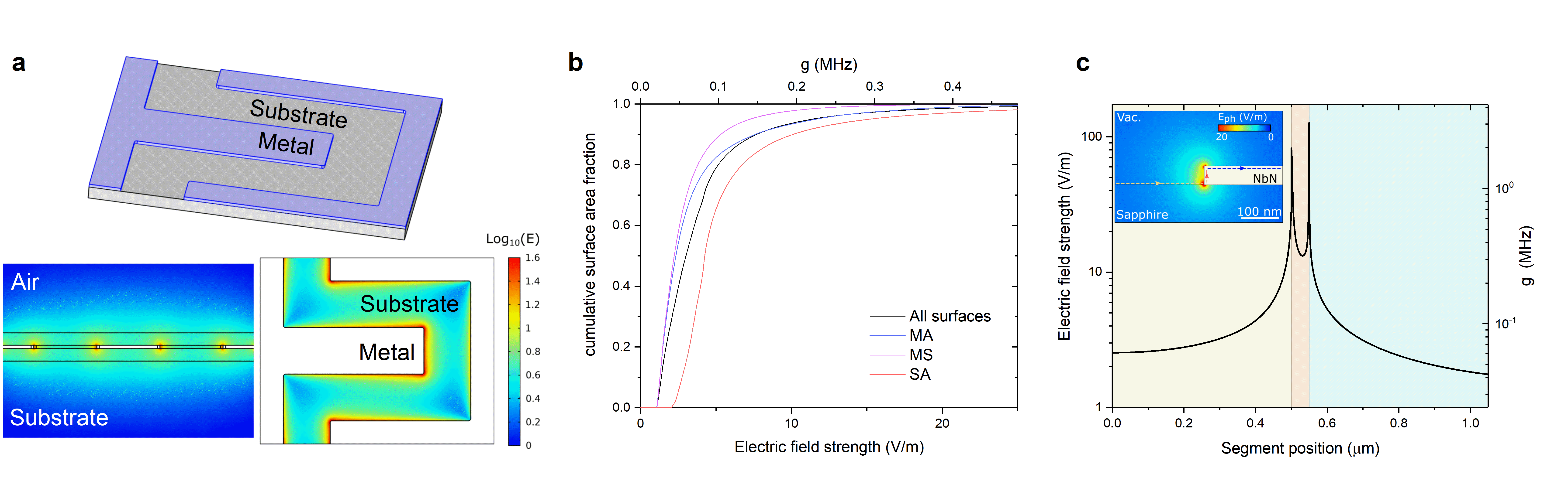
Figure LS13: Microwave electric field strength in the resonator. a) Single photon electric field strengths obtained through a COMSOL simulation for a segment of the resonator, assumed to be at the voltage antinode of the resonator. Top: 3D model of the simulated volume. Bottom left: vertical cross-section showing Electric field strengths. Bottom right: Cross section in the substrate surface plane. b) integrated probability distributions for elenctric field strengths and corresponding resonator-TLS coupling strengths (assuming dipole moment $p_{0}=0.8$ eÅ) for the different device interfaces; Metal-Substrate (MS), Metal-Air (MA) and Substrate-Air (SA). c) Cross-sectional evaluation of the electric field strength near a metal edge showing that significant coupling strengths ($>50$ kHz $\gtrsim f_{0}/Q$) can be obtained across the whole metal surface of the device.

Appendix M qTLS magnetic field measurements

Finally, we here outline the details of the qTLS measurement in mangetic field shown in Fig. 4 of the main manuscript. To measure a coherent qTLS in magnetic field we placed the sample in the bore of a 9/1/1 T vector magnet inside the dilution refrigerator. The resonators themselves are highly magnetic field resilient, retaining quality factors in excess of $10^{5}$ above $B=1$ T. To ensure optimal alignment of the magnetic field with the superconducting plane we applied a small field (5 mT), by rotating the field by a small amount (few degrees) and tracking the resonance frequency as a function of field angle we find the optimal orientation from the maximum in the resonance frequency.

The experiments presented in the main manuscript were carried out at zero current detuning, and we instead tune the TLS into resonance with the resonator using the electrostatic gate in the sample enclosure. The reason for this was purely technical, for larger tuning currents the resonator becomes more sensitive to current noise, and most likely due to mechanical resonances and eddy currents in the coaxial cables excited by the pulse tubes of the cryostat, we saw an increased instability of the resonator frequency at larger magnetic fields. By staying at zero current detuning we minimise this noise.

References

- (1) Klimov, P. V. et al., Fluctuations of energy-relaxation times in superconducting qubits. Phys. Rev. Lett. 121, 090502 (2018).
- (2) de Graaf, S. E. et al., Direct identification of dilute surface spins on Al2O3: origin of flux noise in quantum circuits. Phys. Rev. Lett. 118, 057703 (2017).
- (3) Burnett, J. et al., Evidence for interacting two-level systems from the 1/f noise of a superconducting resonator. Nature Communications 5, 4119 (2014).
- (4) Bilmes, A. et al., Resolving the positions of defects in superconducting quantum bits. Sci. Rep. 10, 3090 (2020).
- (5) Lisenfeld, J. et al., Electric field spectroscopy of material defects in transmon qubits. npj Quantum Information 5, 105 (2019).
- (6) Arute, F. et al., Quantum supremacy using a programmable superconducting processor. Nature 574, 505510 (2019).
- (7) Schlör, S. et al., Correlating decoherence in transmon qubits: low frequency noise by single fluctuators. Phys. Rev. Lett. 123, 190502 (2019).
- (8) Burnett, J. et al., Decoherence benchmarking of superconducting qubits. npj Quantum Information 5, 54 (2019).
- (9) de Graaf, S. E. et al., Suppression of low-frequency charge noise in superconducting resonators by surface spin desorption. Nature Communications 9, 1143 (2018).
- (10) Schneider, A. et al., Transmon qubit in a magnetic field: evolution of coherence and transition frequency. Phys. Rev. Research 1, 023003 (2019).
- (11) Grabovskij, G. J. , Peichl, T., Lisenfeld, J., Weiss, G., and Ustinov, A. V., Strain tuning of individual atomic tunneling systems detected by a superconducting qubit. Science, 338, 232 (2012).
- (12) Geaney, S. et al., Near-field scanning microwave microscopy in the single photon regime. Sci. Rep. 9, 12539 (2019).
- (13) de Graaf, S. E. , Danilov, A. V., and Kubatkin, S. E., Coherent interaction with two-level fluctuators using near field scanning microwave microscopy. Sci. Rep. 5, 17176 (2015).
- (14) Lisenfeld, J. et al., Observation of directly interacting coherent two-level systems in an amorphous material. Nature Communications 6, 6182 (2015).
- (15) Lisenfeld, J. et al., Decoherence spectroscopy with individual two-level tunneling defects. Sci. Rep. 6:23786 (2016).
- (16) Serniak, K. et al., Hot nonequilibrium quasiparticles in transmon qubits. Phys. Rev. Lett., 121, 157701 (2018).
- (17) Henriques, F. et al., Phonon traps reduce the quasiparticle density in superconducting circuits. Appl. Phys. Lett. 115, 212601 (2019).
- (18) Jin, X. Y. et al., Thermal and residual excited-state population in a 3d transmon qubit. Phys. Rev. Lett. 114, 240501 (2015).
- (19) de Visser, P. J. et al., Microwave-induced excess quasiparticles in superconducting resonators measured through correlated conductivity fluctuations. Appl. Phys. Lett. 100, 162601 (2012).
- (20) Moore, D. C. et al., Position and energy-resolved particle detection using phonon-mediated microwave kinetic inductance detectors. Appl. Phys. Lett. 100, 232601 (2012).
- (21) Carbillet, C. et al., Spectroscopic evidence for strong correlations between local resistance and superconducting gap in ultrathin NbN films. Arxiv preprint, 1903.01802 (2019).
- (22) Lemarié, G. et al., Universal scaling of the order-parameter distribution in strongly disordered superconductors. Phys. Rev. B, 87, 184509 (2013).
- (23) Liao, W.-T. et al., Scanning tunneling Andreev microscopy of titanium nitride thin films. Phys. Rev. B 100, 214505 (2019).
- (24) Saveskul, N. A. et al., Superconductivity behavior in epitaxial TiN films points to surface magnetic disorder. Phys. Rev. Appl. 12, 054001 (2019).
- (25) Anton, S. M. et al., Magnetic flux noise in DC SQUIDs: temperature and geometry dependence. Phys. Rev. Lett. 110, 147002 (2013).
- (26) Paladino, E., Galperin, Y. M., Falci G., and Altshhuler, B. L., 1/f noise: Implications for solid-state quantum information. Rev. Mod. Phys. 86, 361-418 (2014).
- (27) Quintana, C. M. et al., Observation of classical-quantum crossover of 1/f flux noise and its paramagnetic temperature dependence. Phys. Rev. Lett. 118, 057702 (2017).
- (28) Müller, C., Cole, J. H., and Lisenfeld, J., Towards understanding two-level-systems in amorphous solids - insights from quantum devices. Prog. Phys. 82, 124501 (2019).
- (29) Kumar, P. et al., Origin and suppression of 1/f magnetic flux noise. Phys. Rev. Appl. 6, 041001 (2016).
- (30) Altshuler, B. L., and Aronov, A. G., in Electron-electron interactions in disordered systems, edited by Efros, A. L., and Pollak, M. (North Holland, Amsterdam, 1985).
- (31) Ivry, Y. et al., Universal scaling of the critical temperature for thin films near the superconducting-to-insulating transition. Phys. Rev. B 90, 214515 (2014).
- (32) Chubov, P., Eremenko, V., and Pilipenko, Y. A., Dependence of the critical temperature and energy gap on the thickness of superconducting aluminum films. Sov. Phys. JETP 28 , 389 (1969).
- (33) Wong, C. H. et al., The role of the coherence length for the establishment of global phase coherence in arrays of ultra-thin superconducting nanowires. Supercond. Sci. Tech. 30, 105004 (2017).
- (34) Mahashabde, S. et al., Fast tunable high Q-factor superconducting microwave resonators. Arxiv preprint 2003.11068.
- (35) Phillips, W. A., Two-level states in glasses. Rep. Prog. Phys. 50, 1657-1708 (1987).
- (36) See Supplemental Material for additional data and methodology, including also references Fominov2011 ; proslier2008 ; huang2019 ; heinrich2017 ; tobiaspound ; burnett2016 .
- (37) Larkin, A. I., and Ovchinnikov, Yu. N., Density of states in inhomogeneous superconductors. Soviet Physics JETP 34, 1144 (1972).
- (38) Lamacraft, A., and Simons, B. D., Tail states in a superconductor with magnetic impurities. Phys. Rev. Lett. 85, 4783 (2000).
- (39) Silva, A., and Ioffe, L. B., Subgap states in dirty superconductors and their effect on dephasing in Josephson qubits. Phys. Rev. B 71, 104502 (2005).
- (40) Halperin, B. I., and Lax, M., Impurity-band tails in the high-density limit. I. minimum counting methods. Phys. Rev. 148, 722 (1966).
- (41) Cardy, J. L., Electron localisation in disordered systems and classical solutions in Ginzburg-Landau field theory. J. Phys. C11, L321 (1978).
- (42) Brown, N. C., Newman, M., and Brown, K. R., Handling leakage with subsystem codes. New J. Phys. 21 073055 (2019).
- (43) Faoro, L., and Ioffe, L. B., Interacting tunneling model for two-level systems in amorphous materials and its predictions for their dephasing and noise in superconducting microresonators. Phys. Rev. B 91, 014201 (2015).
- (44) Churkin, A., Matityahu, S., Maksymov, A. O., Burin, A. L., and Schechter, M., Anomalous low-energy properties in amorphous solids and the interplay of electric and elastic interactions of tunneling two-level systems. arxiv preprint 2002.02877.
- (45) Sarabi, B., Ramanayaka, A. N., Burin, A. L., Wellstood, F. C., and Osborn, K. D., Projected dipole moments of individual two-level defects extracted using circuit quantum electrodynamics. Phys. Rev. Lett. 116, 167002 (2016).
- (46) de Graaf, S. E., Tzalenchuk, A. Ya., and Lindström, T., 1/f frequency noise of superconducting resonators in large magnetic fields. Appl. Phys. Lett. 113, 142601 (2018).
- (47) Yan, F. et al., The flux qubit revisited to enhance coherence and reproducibility. Nature Communications 7, 12964 (2016).
- (48) Nguyen, L. B. et al., High-coherence fluxonium qubit. Phys. Rev. X, 9, 041041 (2019).
- (49) Quintana, C. M., Superconducting flux qubits for high-connectivity quantum annealing without lossy dielectrics, University of California Santa Barbara (2017).
- (50) McDermott, R. F. et al., to be published.
- (51) Karatsu, K. et al., Mitigation of cosmic ray effect on microwave kinetic inductance detector arrays. Appl. Phys. Lett. 114, 032601 (2019).
- (52) Fominov, Ya. V., Houzet, M., and Glazman, L. I., Surface impedance of superconductors with weak magnetic impurities. Phys. Rev. B 84, 224517 (2011).
- (53) Proslier, T. et al., Tunneling study of cavity grade Nb: Possible magnetic scattering at the surface. Appl. Phys. Lett. 92, 212505 (2008).
- (54) Huang, H., Tunneling dynamics between superconducting bound states at the atomic limit. arXiv preprint 1912.08901.
- (55) Heinrich, B. W., Pascual, J. I., and Franke, K. J., Single magnetic adsorbates on s-wave superconductors. Prog. Surf. Sci. 93, 1-19 (2018).
- (56) Lindström, T., Burnett, J., Oxborrow, M., and Tzalenchuk, A. Ya., Pound-locking for characterization of superconducting microresonators. Rev. Sci. Instrum. 82, 104706 (2011).
- (57) Burnett, J., Faoro, L., and Lindström, T., Analysis of high quality superconducting resonators: consequences for TLS properties in amorphous oxides. Supercond. Sci. Technol. 29, 044008 (2016).