Three-dimensional phase transitions in multiflavor lattice scalar SO($N_{c}$) gauge theories

Abstract

We investigate the phase diagram and finite-temperature transitions of three-dimensional scalar SO($N_{c}$) gauge theories with $N_{f}\geq 2$ scalar flavors. These models are constructed starting from a maximally O($N$)-symmetric multicomponent scalar model ($N=N_{c}N_{f}$), whose symmetry is partially gauged to obtain an SO($N_{c}$) gauge theory, with O($N_{f}$) or U($N_{f})$ global symmetry for $N_{c}\geq 3$ or $N_{c}=2$, respectively. These systems undergo finite-temperature transitions, where the global symmetry is broken. Their nature is discussed using the Landau-Ginzburg-Wilson (LGW) approach, based on a gauge-invariant order parameter, and the continuum scalar SO($N_{c}$) gauge theory. The LGW approach predicts that the transition is of first order for $N_{f}\geq 3$. For $N_{f}=2$ the transition is predicted to be continuous: it belongs to the O(3) vector universality class for $N_{c}=2$ and to the $XY$ universality class for any $N_{c}\geq 3$. We perform numerical simulations for $N_{c}=3$ and $N_{f}=2,3$. The numerical results are in agreement with the LGW predictions.

I Introduction

Global and local gauge symmetries play a crucial role in theories describing fundamental interactions Weinberg-book and emerging phenomena in condensed matter physics Sachdev-19 . Interacting scalar fields with local gauge symmetries provide paradigmatic examples for the Higgs mechanism at the basis of superconductivity Anderson-63 and of the Standard Model of the fundamental interactions SSBgauge . In condensed matter physics, they may be relevant for systems with emerging nonabelian gauge symmetries, see, e.g., Refs. GASVW-18 ; SSST-19 . The interplay between global and local gauge symmetries turns out to be crucial to determine their phase diagram, the nature and universality classes (if the transition is continuous) of their thermal and quantum transitions.

These issues have been recently investigated in multicomponent lattice Abelian-Higgs models PV-19-2 ; BPV-19-2d and in multiflavor lattice scalar models with SU($N_{c}$) gauge symmetry BPV-19 ; BPV-20-3d ; SPSS-20 ; BPV-20-2d . For three-dimensional (3D) systems, the nature of the phase transitions turns out to be effectively described by Landau-Ginzburg-Wilson (LGW) $\Phi^{4}$ theories based on a gauge-invariant order-parameter field, that have the same global symmetry as the lattice model. The LGW approach is expected to be effective when the gauge interactions are short-ranged at the transition and can therefore be neglected in the effective model that encodes the long-range modes. In the opposite case, when gauge correlations become critical as well, other theories may be more appropriate, such as continuum gauge theories in which gauge fields are explicitly present.

In this paper we return on this issue, to deepen our understanding of the role that global and local nonabelian symmetries play in determining the main features of the phase diagram and the nature of the phase transitions. For this purpose, we consider a multiflavor 3D lattice scalar model characterized by an SO($N_{c}$) gauge symmetry and an O($N_{f}$) global symmetry, using the standard Wilson formulation Wilson-74 . The model is defined starting from an O($N$)-symmetric scalar model with $N=N_{f}N_{c}$. The global O($N$) symmetry is partially gauged, obtaining a nonabelian gauge model, in which the fields belong to the coset $S^{N}$/SO($N_{c}$), where $S^{N}=\hbox{SO}(N)/\hbox{SO}(N-1)$ is the $N$-dimensional sphere.

In this paper, we shall show that the phase diagrams of multiflavor lattice SO($N_{c}$) gauge models present two phases, which can be characterized by using a rank-two real order parameter, whose condensation breaks the global symmetry. To identify the nature of the phase transition, which separates the two phases, we consider two different field-theoretical approaches: the effective LGW theory, based on a gauge-invariant order-parameter field, and the continuum multiflavor scalar SO($N_{c}$) gauge theory with explicit nonabelian gauge fields. Their predictions are compared with numerical Monte Carlo (MC) results. As it was the case for the multiflavor lattice scalar chromodynamics characterized by an SU($N_{c}$) gauge symmetry BPV-19 ; BPV-20-3d and for the multicomponent lattice Abelian-Higgs model with U(1) gauge symmetry PV-19-2 , a detailed finite-size scaling (FSS) analysis of the numerical results supports the LGW predictions. We recall that an analogous LGW approach was originally used to predict the nature of the finite-temperature phase transition of hadronic matter in the limit of massless quarks, implicitly assuming that the SU(3) gauge modes are not critical PW-84 ; BPV-03 ; PV-13 .

The paper is organized as follows. In Sec. II the lattice model is introduced, with a discussion of its global and local symmetry. In Sec. III we define the LGW $\Phi^{4}$ theory appropriate for the model and the continuum scalar SO($N_{c}$) gauge theory and discuss their predictions for the nature of the transitions. In Sec. IV we report MC results for $N_{c}=3$ and $N_{f}=2,3$, and the FSS analyses that we perform to ascertain the nature of the phase transitions. Finally, we summarize and draw our conclusions in Sec. V.

II The lattice model

We consider a 3D lattice model defined in terms of $N_{c}\times N_{f}$ real matrix variables $\varphi^{af}_{\bm{x}}$ associated with each site ${\bm{x}}$ of a cubic lattice. We start from a maximally symmetric model with action

$$S_{\rm inv}=-\sum_{{\bm{x}},\mu}{\rm Tr}\,\varphi_{\bm{x}}^{t}\varphi_{{\bm{x}}+\hat{\mu}}+\sum_{\bm{x}}V({\rm Tr}\varphi_{\bm{x}}^{t}\,\varphi_{\bm{x}})\,,$$ (1)

$$V(X)=r\,X+{1\over 2}u\,X^{2}\,,$$ (2)

where the first sum is over the lattice links, the second one is over the lattice sites, and $\hat{\mu}=\hat{1},\hat{2},\hat{3}$ are unit vectors along the three lattice directions. In this paper we consider unit-length variables satisfying

$${\rm Tr}\,\varphi_{\bm{x}}^{t}\varphi_{\bm{x}}=1\,,$$ (3)

so that the action is simply

$$S_{\rm inv}=-\sum_{{\bm{x}},\mu}{\rm Tr}\,\varphi_{\bm{x}}^{t}\varphi_{{\bm{x}}+\hat{\mu}}\,.$$ (4)

Formally, the model can be obtained setting $r=-u$, and taking the limit $u\to\infty$ of the potential (2). Models with actions (1) and (4) are invariant under O($N$) transformations with $N=N_{c}N_{f}$. This is immediately checked if we express the matrices $\varphi_{\bm{x}}$ in terms of $N$-component real vectors ${\bm{S}}_{\bm{x}}$. In the new variables we obtain the standard action of the O($N$) nonlinear $\sigma$-model

$$S_{N}=-\sum_{{\bm{x}},\mu}{\bm{S}}_{\bm{x}}\cdot{\bm{S}}_{{\bm{x}}+\hat{\mu}}\,,\qquad{\bm{S}}_{\bm{x}}\cdot{\bm{S}}_{\bm{x}}=1\,.$$ (5)

We now proceed by gauging some of the degrees of freedom: we associate an SO($N_{c}$) matrix $V_{{\bm{x}},\mu}$ with each lattice link and extend the action (4) to ensure SO($N_{c}$) gauge invariance. We also add a kinetic term for the gauge variables in the Wilson form Wilson-74 . We thus obtain the model with action

$$S_{g} =-N_{f}\sum_{{\bm{x}},\mu}{\rm Tr}\left[\varphi_{\bm{x}}^{t}\,V_{{\bm{x}},{\mu}}\,\varphi_{{\bm{x}}+\hat{\mu}}\right]$$ (6)

$$-{\gamma\over N_{c}}\sum_{{\bm{x}},\mu>\nu}{\rm Tr}\,\left[V_{{\bm{x}},{\mu}}\,V_{{\bm{x}}+\hat{\mu},{\nu}}\,V_{{\bm{x}}+\hat{\nu},{\mu}}^{t}\,V_{{\bm{x}},{\nu}}^{t}\right]\,,$$

and partition function

$$Z=\sum_{\{\varphi,V\}}e^{-\beta S_{g}}\,.$$ (7)

Note that, for $\gamma\to\infty$, the product of the gauge fields along a plaquette converges to one. This implies that $V_{{\bm{x}},\mu}=1$ modulo a gauge transformation. Therefore, in the $\gamma\to\infty$ limit we reobtain the O($N$) invariant theory (4) we started from. For any value of $N_{c}$ and $N_{f}$, $S_{g}$ is invariant under the local gauge transformation $\varphi_{\bm{x}}\to G_{\bm{x}}\varphi_{\bm{x}}$ and $V_{\bm{x},{\mu}}\to G_{\bm{x}}V_{\bm{x},{\mu}}G_{\bm{x}+\hat{\mu}}^{t}$ with $G_{\bm{x}}\in$ SO($N_{c}$), and under the global transformation $\varphi_{\bm{x}}\to\varphi_{\bm{x}}W$ and $V_{\bm{x},{\mu}}\to V_{\bm{x},{\mu}}$ with $W\in$ O($N_{f}$).

For $N_{c}=2$ the global symmetry is actually larger than O($N_{f}$). We write $V_{{\bm{x}},\mu}\in$ SO(2) as

$$V_{{\bm{x}},\mu}=\begin{pmatrix}\cos\theta_{{\bm{x}},\mu}&\sin\theta_{{\bm{x}},\mu}\\ -\sin\theta_{{\bm{x}},\mu}&\cos\theta_{{\bm{x}},\mu}\end{pmatrix}\,,$$ (8)

we define a complex $N_{f}$-dimensional vector

$${z}^{f}_{\bm{x}}=\varphi^{1f}_{\bm{x}}+i\varphi^{2f}_{\bm{x}}\,,$$ (9)

which satisfies $\bar{\bm{z}}_{\bm{x}}\cdot{\bm{z}}_{\bm{x}}=1$ because of Eq. (3), and the U(1) link variable $\lambda_{{\bm{x}},\mu}\equiv e^{i\theta_{{\bm{x}},\mu}}$. In terms of the new variables, the lattice action (6) becomes

$$S_{\rm AH}=-\,\sum_{{\bm{x}},\mu}{\rm Re}\,[\bar{\bm{z}}_{\bm{x}}\cdot\lambda_{{\bm{x}},\mu}\,{\bm{z}}_{{\bm{x}}+\hat{\mu}}]$$ (10)

$$\qquad-\gamma\sum_{{\bm{x}},\mu>\nu}{\rm Re}\,[\lambda_{{\bm{x}},{\mu}}\,\lambda_{{\bm{x}}+\hat{\mu},{\nu}}\,\bar{\lambda}_{{\bm{x}}+\hat{\nu},{\mu}}\,\bar{\lambda}_{{\bm{x}},{\nu}}]\,.$$

This is the action of the $N_{f}$-component lattice Abelian-Higgs model, which is invariant under local U(1) and global U$(N_{f})$ transformations. There is therefore an enlargement of the global symmetry of the model: the global symmetry group is U$(N_{f})$ instead of O($N_{f}$). The phase structure of the Abelian-Higgs model (10) has been studied in detail in Ref. PV-19-2 . Therefore, in this work we will focus on the behavior for $N_{c}\geq 3$.

It is interesting to note that one can consider more general Hamiltonians that have the same global and local invariance. Indeed, one can start from a Hamiltonian in which the potential is any O($N_{f}$)-invariant function of $\varphi^{t}\varphi$. For instance, if we only consider quartic potentials in $\varphi_{\bm{x}}$, we can take

$$V_{g}(\varphi)=V(X)+v\,\{{\rm Tr}[\varphi_{\bm{x}}^{t}\,\varphi_{\bm{x}}\,\varphi_{\bm{x}}^{t}\,\varphi_{\bm{x}}]-({\rm Tr}[\varphi_{\bm{x}}^{t}\,\varphi_{\bm{x}}])^{2}\}\,.$$ (11)

If we consider this class of more general Hamiltonians, there is no enlargement of the symmetry from O($N_{f}$) to O($N$) in the limit $\gamma\to\infty$, in which gauge degrees of freedom are frozen. Moreover, for $N_{c}=2$, the symmetry enlargement from O$(N_{f})$ to U($N_{f}$) does not occur.

Since the global symmetry group O($N_{f}$) corresponds to SO($N_{f})\times{\mathbb{Z}}_{2}$, there is the possibility of breaking separately the two different groups. In this work we will focus on the breaking of the SO($N_{f}$) subgroup, which, by analogy with our results for complex U($N_{f}$) invariant gauge models BPV-20-3d , is expected to be the only one occurring in the model with action (6). However, the ${\mathbb{Z}}_{2}$ symmetry may play a role in more general models, for instance in those with action (11), in which the breaking of both the ${\mathbb{Z}}_{2}$ and the SO($N_{f}$) subgroups may occur. Note that the presence of two possible symmetry breaking patterns is related to the fact that the gauge symmetry group is SO($N_{c}$). Had we considered an O($N_{c}$) gauge invariant model, we would have only an SO($N_{f}$) global invariance.

The natural order parameter for the breaking of the SO($N_{f}$) global symmetry group is the gauge-invariant real traceless and symmetric bilinear operator

$$Q^{fg}_{\bm{x}}=\sum_{a}\varphi^{af}_{\bm{x}}\varphi^{ag}_{\bm{x}}-{\delta^{fg}\over N_{f}}\,,$$ (12)

which is a rank-2 operator with respect to the global O($N_{f}$) symmetry group. As we shall show, the phase diagram of the model ($N_{c}\geq 3$) presents two different phases, separated by a phase-transition line associated with the condensation of the bilinear $Q$.

We finally mention that, for $N_{f}=1$, the phase diagram of the lattice scalar SO($N_{c}$) gauge model (6) is expected to show only one phase. This can be easily verified for $\gamma=0$. In this case the $N_{f}=1$ model is trivial and cannot have any phase transition.

III Effective field theories

III.1 The LGW field theory

To characterize the finite-temperature transitions of scalar SO($N_{c}$) gauge theories, we consider the LGW approach Landau-book ; WK-74 ; Fisher-75 ; ZJ-book . We start by considering an order parameter that breaks the global symmetry of the model. For $N_{c}\geq 3$, the global symmetry group is O($N_{f}$) and an appropriate order parameter is the bilinear tensor $Q_{\bm{x}}$ defined in Eq. (12). The corresponding LGW theory is obtained by considering a real symmetric traceless $N_{f}\times N_{f}$ matrix field $\Phi({\bm{x}})$, which represents a coarse-grained version of $Q_{\bm{x}}$. The Lagrangian is

$${\cal L}_{\rm LGW} = \hbox{Tr }\partial_{\mu}\Phi\partial_{\mu}\Phi+r\,\hbox{Tr }\Phi^{2}+\,u_{3}\,\hbox{Tr }\Phi^{3}\qquad$$ (13)

$$+\,u_{41}\,\hbox{Tr }\Phi^{4}+u_{42}\,(\hbox{Tr }\Phi^{2})^{2}\,,$$

where the potential is the most general O($N_{f}$)-invariant fourth-order polynomial in the field. The Lagrangian (13) is invariant under the global transformations

$$\Phi\to W\Phi W^{t}\,,\qquad W\in{\rm O}(N_{f})\,.$$ (14)

The renormalization-group (RG) flow of model (13) has been already discussed in Ref. PTV-18 . For $N_{f}=2$ the cubic term vanishes and the two quartic terms are proportional, so that we obtain the two-component vector $\Phi^{4}$ action. Therefore, for $N_{f}=2$ the system may undergo a continuous transition in the $XY$ universality class. For $N_{f}>2$ the cubic term is generically present. Assuming that the usual mean-field arguments, valid close to four dimensions, apply also to the three-dimensional case, only first-order transitions are expected. A continuous transition is only possible if the Hamiltonian parameters are tuned or an additional symmetry is present, so that the cubic term vanishes. If this occurs, we obtain the LGW model discussed in Ref. PTV-18 , in the context of the antiferromagnetic RP${}^{N_{f}-1}$ model. In particular, for $N_{f}=3$, the LGW theory is equivalent to that of the O(5) vector model PTV-18 ; FMSTV-05 , so that continuous transitions in the O(5) universality class may occur.

The previous conclusions also hold for $N_{c}=2$ for generic actions with SO($N_{f}$) global symmetry, for instance for the action (11). On the other hand, for our model (6) the previous results do not hold for $N_{c}=2$, because of the symmetry enlargement to U($N_{f}$). In this case the LGW field is a Hermitean traceless $N_{f}\times N_{f}$ matrix field DPV-15 ; PV-19 with a Lagrangian that is the analogue of the one considered here, Eq. (13). Its RG flow predicts that PV-19-2 the transition can be continuous for $N_{f}=2$, in the O(3) vector universality class, while it is of first order for $N_{f}\geq 3$.

The above-reported discussion applies to any model in which the global symmetry group is SO($N_{f}$) and the order parameter is a real operator that transforms as a rank-two tensor under SO($N_{f}$) transformations. Therefore, the results apply to other scalar models and, in particular, to scalar SU(2) gauge theories with scalar fields in the adjoint representation, which have been recently considered to describe the critical behavior of cuprate superconductors for optimal doping SSST-19 ; SPSS-20 . In these theories the fundamental fields are $N_{h}$ Higgs fields transforming under the adjoint representation of SU(2), i.e. $\hat{\phi}^{f}_{\bm{x}}\equiv\sum_{a=1}^{3}\phi_{\bm{x}}^{af}\tau^{a}$, where $\tau^{a}\equiv\sigma^{a}/2$, $\sigma^{a}$ are the Pauli matrices and $f=1,...,N_{h}$. In the fixed-length limit ${\rm Tr}[\phi_{\bm{x}}^{t}\phi_{\bm{x}}]=1$, the lattice action is Laine-95 ; SPSS-20

$$S_{h} =-\sum_{{\bm{x}},\mu,f}{\rm Tr}\left[\hat{\phi}^{f}_{\bm{x}}U_{{\bm{x}},{\mu}}\hat{\phi}^{f}_{{\bm{x}}+\hat{\mu}}U_{{\bm{x}},{\mu}}^{\dagger}\right]$$ (15)

$$-{\gamma\over 2}\sum_{{\bm{x}},\mu>\nu}{\rm Tr}\,\left[U_{{\bm{x}},{\mu}}\,U_{{\bm{x}}+\hat{\mu},{\nu}}\,U_{{\bm{x}}+\hat{\nu},{\mu}}^{t}\,U_{{\bm{x}},{\nu}}^{t}\right]$$

$$+u\sum_{\bm{x}}{\rm Tr}[\phi_{\bm{x}}^{t}\phi_{\bm{x}}\phi_{\bm{x}}^{t}\phi_{\bm{x}}]\,,$$

where $U_{{\bm{x}},{\mu}}$ are SU(2) link variables. For any $N_{h}$, the action $S_{h}$ is invariant under the local SU(2) gauge transformation $\hat{\phi}_{\bm{x}}^{f}\to G_{\bm{x}}\hat{\phi}_{\bm{x}}^{f}G_{\bm{x}}^{\dagger}$ and $U_{\bm{x},{\mu}}\to G_{\bm{x}}U_{\bm{x},{\mu}}G_{\bm{x}+\hat{\mu}}^{\dagger}$ with $G_{\bm{x}}\in$ SU(2), and under the global transformation $\phi_{\bm{x}}\to\phi_{\bm{x}}W$ with $W\in\,$O($N_{h}$). The appropriate order parameter is again a gauge-invariant operator which transforms as a rank-two traceless real tensor with respect to the global O($N_{h}$) symmetry,

$${\cal Q}^{fg}_{\bm{x}}=\sum_{a}\phi^{af}_{\bm{x}}\phi^{ag}_{\bm{x}}-{\delta^{fg}\over N_{h}}\,.$$ (16)

The corresponding LGW action is again Eq. (13). Therefore, for $N_{h}=2$ transitions associated with the breaking of the O($N_{h}$) symmetry may be continuous in the $XY$ universality class. For $N_{h}\geq 3$ only first-order transitions are possible.

III.2 The continuum scalar SO($N_{c}$) gauge theory

The continuum scalar SO($N_{c}$) gauge theory provides another effective theory for the lattice model (6). Its Lagrangian is obtained by considering all monomials up to dimension four, which can be constructed using the scalar field $\Phi_{af}$ (with $a=1,...,N_{c}$ and $f=1,...,N_{f}$). Gauge invariance is obtained as usual, by adding a gauge field $A_{\mu,ab}\equiv{\cal A}_{\mu}^{k}T_{ab}^{k}$, where the matrices $T^{k}$ are the generators of the SO($N_{c}$) gauge algebra. The Lagrangian reads Hikami-80 ; PRV-01

$${\cal L}={1\over 4}F_{\mu\nu}^{2}+{1\over 2}\sum_{af\mu}(\partial_{\mu}\Phi_{af}+g_{0}A_{\mu,ab}\Phi_{bf})^{2}$$ (17)

$$\quad+{1\over 2}r_{0}\sum_{af}\Phi_{af}^{2}+{1\over 4!}u_{0}(\sum_{af}\Phi_{af}^{2})^{2}$$

$$\quad+{1\over 4!}v_{0}\left[\sum_{abf}\Phi_{af}^{2}\Phi_{bf}^{2}-(\sum_{af}\Phi_{af}^{2})^{2}\right]\,,$$

where $F_{\mu\nu}$ is the non-Abelian field strength associated with the gauge field $A_{\mu,ab}$.

To determine the nature of the transitions described by the continuum SO($N_{c}$) gauge theory (17), one studies the RG flow determined by the $\beta$ functions of the model. In the $\epsilon$-expansion framework, the one-loop $\overline{\rm MS}$ $\beta$ functions control the RG flow close to four dimensions. Introducing the renormalized couplings $u$, $v$, and $\alpha=g^{2}$, the one-loop $\beta$ functions are (see Ref. Hikami-80 for the exact normalizations of the renormalized couplings)

$$\beta_{u}=-\epsilon u+{N_{f}N_{c}+8\over 6}u^{2}+{(N_{f}-1)(N_{c}-1)\over 6}(v^{2}-2uv)$$

$$\qquad-{3\over 2}(N_{c}-1)u\alpha+{9\over 8}(N_{c}-1)\alpha^{2}\,,$$ (18)

$$\beta_{v}=-\epsilon v+{N_{f}+N_{c}-8\over 6}v^{2}+2uv-{3\over 2}(N_{c}-1)v\alpha$$

$$\qquad+{9\over 4}(N_{c}-2)\alpha^{2}\,,$$

$$\beta_{\alpha}=-\epsilon\alpha+{N_{f}-22(N_{c}-2)\over 12}\alpha^{2}\,,$$

where $\epsilon\equiv 4-d$. Note that for $N_{c}=2$ the $\beta$ functions $\beta_{u}$ and $\beta_{\alpha}$ for $v=0$ map exactly onto those of the Abelian-Higgs model HLM-74 ; PV-19-2 , after an appropriate change of normalization of the couplings. We recall that the RG flow of the Abelian-Higgs theory has a stable fixed point only for large $N_{f}$, i.e. $N_{f}>90+24\sqrt{15}+O(\epsilon)$.

The RG flow described by the $\beta$ functions (18) generally predicts first-order transitions, unless the number of flavors is large. In particular, one can easily see that the RG flow described by the $\beta$ functions (18) cannot have stable fixed points for

$$N_{f}<22(N_{c}-2)\,,$$ (19)

for which the fixed points must necessarily have $\alpha=0$, at least sufficiently close to four dimensions. The fixed points with vanishing gauge coupling $\alpha=0$ are always unstable with respect to the gauge coupling, since their stability matrix $\Omega_{ij}=\partial\beta_{i}/\partial g_{j}$ has a a negative eigenvalue

$$\lambda_{\alpha}=\left.{\partial\beta_{\alpha}\over\partial\alpha}\right|_{\alpha=0}=-\epsilon+O(\epsilon^{2})\,.$$ (20)

A more careful analysis shows that, for any $N_{c}$, a nontrivial stable fixed point (with nonzero values of all couplings) exists only for sufficiently large $N_{f}$ Hikami-80 ; PRV-01 . This result is also confirmed by three-dimensional large-$N_{f}$ computations for fixed $N_{c}$  Hikami-80 . Therefore, continuous transitions are only possible for a large number of components.

The above results contradict the LGW predictions. For $N_{f}=2$ the continuum theory predicts a first-order transition, while, according to the LGW analysis, $XY$ continuous transitions are possible. Vice versa, for large $N_{f}$ continuous transitions are possible according to the continuum theory, but not on the basis of the LGW analysis. We note that analogously contradictory results were obtained for the Abelian-Higgs model PV-19-2 and the scalar chromodynamics BPV-19 .

Note that, unlike the LGW theory (13), the RG flow of the continuum scalar SO($N_{c}$) gauge theory (17) presents an unstable O($N$) fixed point with $N=N_{f}N_{c}$, which describes the critical behavior of the lattice model (6) in the $\gamma\to\infty$ limit. This is located at

$$u=\epsilon\,{6\over N_{f}N_{c}+8}+O(\epsilon^{2})\,,\quad v=0\,,\quad\alpha=0\,.$$ (21)

One can easily show that this fixed point is always unstable, even in the absence of gauge interactions. The perturbation associated with the coupling $v$ is a spin-four perturbation at the O($N$) fixed point, which is relevant for any $N\geq 3$ CPV-03 ; HV-11 . Moreover, also the gauge perturbation associated with the coupling $\alpha$ is relevant, as it is associated with a negative eigenvalue $\lambda_{\alpha}=-\epsilon+O(\epsilon^{2})$ of the stability matrix, see Eq. (20).

IV Numerical results

In this section we report numerical results for the lattice scalar SO(3) gauge theory with two and three flavors. We consider cubic lattices of linear size $L$ with periodic boundary conditions. To update the gauge fields we use an overrelaxation algorithm implemented à la Cabibbo-Marinari Cabibbo:1982zn , considering three SO(2) subgroups of SO(3). We use a combination of biased-Metropolis updates and microcanonical steps Creutz:1987xi in the ratio 1:5. For the update of the scalar fields a combination of Metropolis and microcanonical updates is used, with the Metropolis step tuned to have an acceptance rate of approximately 30%.

IV.1 Observables and analysis method

We consider the energy density and the specific heat, defined as

$$E=-\frac{1}{3N_{f}V}\langle S_{g}\rangle\,,\quad C_{V}=\frac{1}{9N_{f}^{2}V}\left(\langle S_{g}^{2}\rangle-\langle S_{g}\rangle^{2}\right)\,,\quad$$ (22)

where $V=L^{3}$. To study the breaking of the O($N_{f}$) flavor symmetry, we consider the order parameter $Q_{\bm{x}}$ defined in Eq. (12). Its two-point correlation function is defined by

$$G({\bm{x}}-{\bm{y}})=\langle{\rm Tr}\,Q_{\bm{x}}Q_{\bm{y}}\rangle\,,$$ (23)

where the translation invariance of the system has been explicitly taken into account. We define the corresponding susceptibility $\chi$ and correlation length $\xi$ as

$$\chi=\sum_{\bm{x}}G({\bm{x}}),\quad\xi^{2}=\frac{1}{4\sin^{2}(\pi/L)}\frac{\widetilde{G}({\bm{0}})-\widetilde{G}({\bm{p}}_{m})}{\widetilde{G}({\bm{p}}_{m})},\quad$$ (24)

where $\widetilde{G}({\bm{p}})=\sum_{{\bm{x}}}e^{i{\bm{p}}\cdot{\bm{x}}}G({\bm{x}})$ is the Fourier transform of $G({\bm{x}})$ and ${\bm{p}}_{m}=(2\pi/L,0,0)$.

At continuous transitions, RG-invariant quantities, such as the Binder parameter

$$U=\frac{\langle\mu_{2}^{2}\rangle}{\langle\mu_{2}\rangle^{2}}\,,\qquad\mu_{2}=\frac{1}{V^{2}}\sum_{{\bm{x}},{\bm{y}}}{\rm Tr}\,Q_{\bm{x}}Q_{\bm{y}}\,,$$ (25)

and

$$R_{\xi}=\xi/L\,,$$ (26)

(which we generically denote by $R$), are expected to scale as PV-02

$$R(\beta,L)=f_{R}(X)+L^{-\omega}g_{R}(X)+\ldots\,,$$ (27)

where $X=(\beta-\beta_{c})L^{1/\nu}$ and next-to-leading scaling corrections have been neglected. The function $f_{R}(X)$ is universal up to a multiplicative rescaling of its argument, $\nu$ is the critical exponent associated with the correlation length, and $\omega$ is the exponent associated with the leading irrelevant operator. In particular, $U^{*}\equiv f_{U}(0)$ and $R_{\xi}^{*}\equiv f_{R_{\xi}}(0)$ are universal, depending only on the boundary conditions and aspect ratio of the lattice. Since $R_{\xi}$ defined in Eq. (26) is an increasing function of $\beta$, we can write

$$U(\beta,L)=F_{U}(R_{\xi})+O(L^{-\omega})\,,$$ (28)

where $F_{U}$ now depends on the universality class, boundary conditions and lattice shape, without any nonuniversal multiplicative factor. The scaling (28) is particularly convenient to test universality-class predictions, since it permits easy comparisons between different models without requiring a tuning of nonuniversal parameters.

In the following we will show that the critical behavior along the phase transition line of two-flavor SO(3) gauge models belongs to the $XY$ universality class, by verifying that the asymptotic FSS behavior of $U$ versus $R_{\xi}$, see Eq. (28), matches that obtained for the $XY$ model. On the other hand, for $N_{f}=3$, we will show that Eq. (28) is not satisfied—the data of $U$ do not scale on a single curve when plotted versus $R_{\xi}$. This can be taken as evidence that the transition is of first order, a conclusion that will be also confirmed by the two-peak structure of the distributions of the energy.

IV.2 The two-flavor lattice SO(3) gauge model

We now present numerical results for the two-flavor SO(3) gauge model (6), showing that it undergoes continuous transitions in the 3D $XY$ universality class, as predicted by the corresponding LGW theory. Some accurate results for the universal quantities of the 3D $XY$ universality class are reported in Table 1.

Ref.	$\nu$	$\eta$	$\omega$	$R_{\xi}^{*}$	$U^{*}$
CHPV-06	0.6717(1)	0.0381(2)	0.785(20)	0.5924(4)	1.2432(2)
Hasenbusch-19	0.67169(7)	0.03810(8)	0.789(4)	0.59238(7)	1.24296(8)
CLLPSSV-19	0.67175(10)	0.038176(44)	0.794(8)

Table 1: Some estimates of the universal critical exponents for the 3D $XY$ universality class, obtained from the analysis of high-temperature expansions supplemented by MC simulations CHPV-06 , from MC simulations Hasenbusch-19 and the conformal-bootstrap approach CLLPSSV-19 . See Ref. PV-02 for earlier theoretical estimates and experimental results. We report the correlation-length exponent $\nu$, the order-parameter exponent $\eta$, the exponent $\omega$ (associated with the leading scaling corrections), and the universal quantities $R_{\xi}^{*}$ and $U^{*}$ (large-$L$ limits of $R_{\xi}$ and $U$ at the critical point, for cubic lattices with periodic boundary conditions).

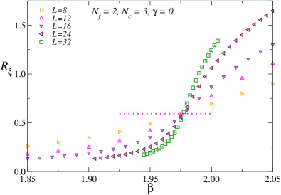
Figure 1: MC data of $R_{\xi}$ versus $\beta$ for the lattice SO(3) gauge model (6) with $N_{f}=2$ and $\gamma=0$. The dotted line corresponds to $R_{\xi}=0.5924$, which is the critical value for the $XY$ universality class, see Table 1.

To begin with, we present results for $\gamma=0$. In Fig. 1 we show the estimates of $R_{\xi}$ for different values of $L$ and $\beta$. The data sets for different values of $L$ clearly display a crossing point, which provides an estimate of the critical point. The data are consistent with the predicted $XY$ behavior. Indeed, the data close to the crossing point nicely fit the simple biased ansatz

$$R_{\xi}=R_{\xi}^{*}+a_{1}X,\quad X=(\beta-\beta_{c})L^{1/\nu},\quad\nu=0.6717,$$ (29)

where $\nu$ is the critical exponent of the $XY$ universality class, see Table 1. Using data within the self-consistent window $R_{\xi}(\beta,L)\in[R_{\xi}^{*}(1-\delta),R_{\xi}^{*}(1+\delta)]$ with $\delta=0.2$, we obtain the estimate $\beta_{c}=1.97690(7)$. The collapse of the data in Fig. 2, where we report the data of $R_{\xi}$ versus $X$, clearly shows the effectiveness of the $XY$ biased fit.

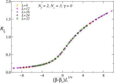
Figure 2: MC data of $R_{\xi}$ versus $(\beta-\beta_{c})L^{1/\nu}$ for the lattice SO(3) gauge model (6) with $N_{f}=2$ and $\gamma=0$. We use $\nu=0.6717$, the value for the $XY$ universality class, see Table 1.

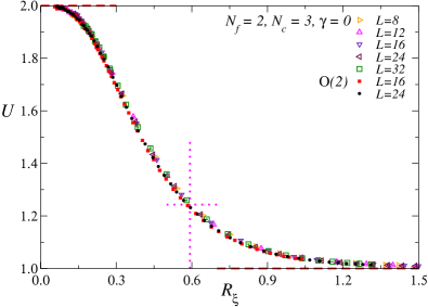
Figure 3: MC data of $U$ versus $R_{\xi}$ for the lattice SO(3) gauge model (6) with $N_{f}=2$ and $\gamma=0$ (data up to $L=32$) and for the $XY$ [O(2)] universality class (data up to $L=24$ for the standard nearest-neighbor $XY$ model). The dotted lines correspond to the universal values $R^{*}_{\xi}$ and $U^{*}$ for the $XY$ universality class, see Table 1.

In Fig. 3 we report results for the Binder parameter $U$ and the ratio $R_{\xi}=\xi/L$. The data of $U$ versus $R_{\xi}$ clearly approach a single curve. which matches the corresponding curve computed in the standard nearest-neighbor $XY$ model with action (5) (again we consider cubic lattices with periodic boundary conditions). This test, which does not require any tuning of free parameters, provides the strongest evidence that the phase transition in the gauge model belongs to the 3D $XY$ universality class. Note that scaling corrections are significantly smaller in the gauge theory than in the standard discretizaton of the $XY$ model, though they are hardly visible in Fig. 3.

We have also checked that $XY$ behavior is also observed for other values of $\gamma$; see Fig. 4, where we report results for $\gamma=3$ and $-3$. This proves the irrelevance of $\gamma$ along the transition line. Of course, a crossover is expected in the limit $\gamma\to\infty$, Indeed, in this limit we should observe an O($N$) critical behavior, with $N=N_{f}N_{c}=6$ (results for the O(6) universality class can be found in Ref. AS-95 ).

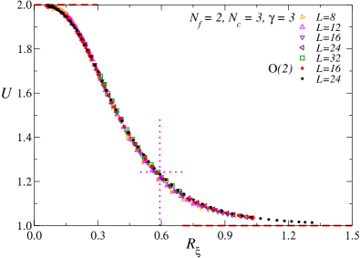
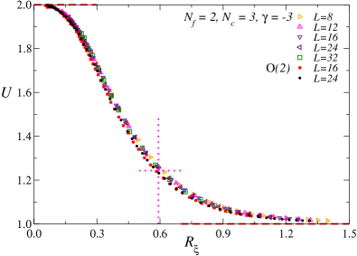
Figure 4: MC data of $U$ versus $R_{\xi}$ for the lattice SO(3) gauge model (6) with $N_{f}=2$ and $\gamma=\pm 3$ (up to $L=32$), and for the $XY$ [O(2)] universality class (data up to $L=24$ for the standard nearest-neighbor $XY$ model). The dotted lines correspond to the universal values $R^{*}_{\xi}$ and $U^{*}$ for the $XY$ universality class, see Table 1.

IV.3 The three-flavor lattice SO(3) gauge model

For $N_{f}=3$ the LGW effective field theory predicts a first-order phase transition for any number of colors. To verify the prediction, we perform simulations for $\gamma=0$.

Figure 5: MC data of $U$ versus $R_{\xi}$ for the lattice SO(3) gauge model (6) with $N_{f}=3$ and $\gamma=0$. The absence of scaling indicates that the transition is not continuous, thus first order.

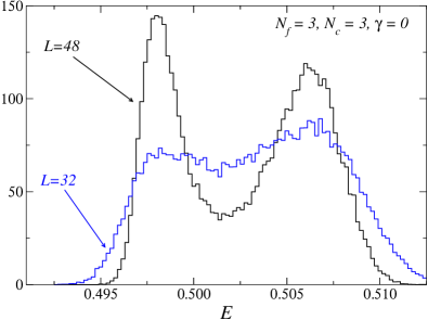
Figure 6: Energy distribution for the lattice SO(3) gauge model (6) with $N_{f}=3$ and $\gamma=0$. We report results for $L=32$ and $L=48$ for $\beta$ values close to the transition. The values of $\beta$ have been selected to obtain two maxima of approximately the same height.

Some evidence in favor of a first-order transition is provided by the analysis of the Binder parameter $U$. At a first-order transition, the maximum $U_{\rm max}$ of $U$ behaves as CLB-86 ; VRSB-93 $U_{\rm max}\sim V$. On the other hand, at a continuous phase transition, $U$ is bounded as $L\to\infty$ and the data of $U$ corresponding to different values of $R_{\xi}$ collapse onto a common scaling curve as the volume is increased. Therefore, $U$ has a qualitatively different scaling behavior for first-order and continuous transitions. In practice, a first-order transition can be identified by verifying that $U_{\rm max}$ increases with $L$, without the need of explicitly observing the linear behavior in the volume. A second indication of a first-order transition is provided by the plot of $U$ versus $R_{\xi}$. The absence of a data collapse is an early indication of the first-order nature of the transition, as already advocated in Ref. PV-19 . In Fig. 5 we plot the Binder parameter $U$ versus $R_{\xi}$. The data, that are obtained at values of $\beta$ close to the transition temperature $\beta_{c}\approx 1.7707$, do not show any scaling. Moreover, $U$ displays a pronounced peak, whose height increases with increasing volume. We take the absence of scaling as an evidence that the transition is of first order.

The first-order transition is also clearly supported by the emergence of a double peak structure in the distribution $P(E)$ of the energy with increasing the lattice size around $\beta_{c}\approx 1.7707$. This is shown in Fig. 6 where the energy histograms for $L=32$ and $L=48$ are compared. Correspondingly the specific heat $C_{V}$ defined in Eq. (22) shows more and more pronounced peaks with increasing $L$ (not shown). However, the expected asymptotic large-volume behaviors, such as $C_{V,{\rm max}}\sim V$ of the maximum value $C_{V,{\rm max}}$ of $C_{V}$, are not clearly observed yet, presumably requiring larger lattice sizes.

We have also considered the gauge-invariant two-point correlation function of the local operator ${\rm det}\,\varphi_{\bm{x}}$ (note that $\varphi^{af}_{\bm{x}}$ is the 3$\times$3 matrix), which may be taken as an order parameter for the ${\mathbb{Z}}_{2}$ global symmetry briefly discussed in Sec. II. The correlation function does not show any qualitative change across the transition. It is always short-ranged, confirming that the ${\mathbb{Z}}_{2}$ global symmetry is not broken and does not play any role at the transition.

In conclusion, the numerical results for $N_{f}=N_{c}=3$ provide a convincing evidence that the transition is of first order for $\gamma=0$. As it occurs for $N_{f}=2$, we conjecture that the nature of the transition does not change in a large interval of values of $\gamma$ around $\gamma=0$. In particular, we conjecture that the transition is of first order for all positive finite values of $\gamma$. Note that, for large $\gamma$, we expect significant crossover effects, since the transition is continuous for $\gamma=\infty$ in the universality class of the O(9) vector $\sigma$-model.

V Summary and conclusions

In this paper we investigate the phase diagram of 3D multiflavor lattice scalar theories in the presence of nonabelian SO($N_{c}$) gauge interactions. We consider the lattice scalar SO($N_{c}$) gauge theory (6) with $N_{f}$ flavors, defined starting from a maximally O($N$)-symmetric multicomponent scalar model ($N=N_{f}N_{c}$). The global O($N$) symmetry is partially gauged, obtaining a gauge model, in which the fields belong to the coset $S^{N}$/SO($N_{c}$), where $S^{N}$ is the $N$-dimensional sphere. Note that, for $N_{c}=2$, the action (6) exactly maps onto that of the $N_{f}$-component lattice Abelian-Higgs model characterized by a U(1) gauge symmetry, whose phase diagram has been studied in Refs. PV-19-2 ; PV-19 . We thus focus on models with $N_{c}\geq 3$.

Figure 7: Sketch of the phase diagram of the 3D lattice scalar SO($N_{c}$) gauge theory (6) with $N_{f}$ flavors and O($N_{f}$) global symmetry. The transition line is continuous for $N_{f}=2$—it belongs to the $XY$ universality class for $N_{c}\geq 3$ and to the O(3) universality class for $N_{c}=2$—and is of first order for $N_{f}\geq 3$. We conjecture that its nature is the same for any finite $\gamma$. The endpoint for $\gamma\to\infty$ is the O($N$) critical point ($N=N_{c}N_{f}$).

For $N_{f}\geq 2$ the phase diagram is characterized by two phases: a low-temperature phase in which the order parameter $Q_{\bm{x}}^{fg}$ defined in Eq. (12) condenses, and a high-temperature disordered phase. The two phases are separated by a transition line, where the SO$(N_{f})$ symmetry is broken, as sketched in Fig. 7. The line ends at the unstable O($N$) transition point with $N=N_{c}N_{f}$ for $\gamma\to\infty$. The gauge parameter $\gamma$, corresponding to the inverse gauge coupling, does not play any particular role: the nature of the transition is conjectured to be the same for any $\gamma$. We have numerically verified this conjecture for two values of $\gamma$. Along the transition line only the correlations of the gauge-invariant operator $Q_{\bm{x}}^{fg}$ are critical, while gauge modes are not critical and only represent a background that gives rise to crossover effects.

The nature of the finite-temperature transitions can be investigated using different field-theoretical approaches. On one side, one can use the effective LGW theory with Lagrangian (13). In this approach based on a gauge-invariant order parameter, only the global symmetry group SO($N_{f}$) and the nature of the order parameter (a rank-two symmetric real traceless tensor) play a role. The gauge degrees of freedom are absent in the effective model. A second approach is based on the continuum SO($N_{c}$) gauge theory, in which the gauge fields are explicitly present. As it occurs for the lattice scalar chromodynamics characterized by an SU($N_{c}$) gauge symmetry BPV-19 ; BPV-20-3d , the numerical results agree with the LGW predictions. The LGW framework provides the correct description of the large-scale behavior of these systems, predicting first-order transitions for $N_{f}=3$, and continuous transitions for $N_{f}=2$, which belong to the $XY$ universality class for any $N_{c}\geq 3$.

The results for $N_{f}=2$ are in contradiction with the predictions of the continuum gauge model (6): since no stable FP exists for $N_{f}=2$, one would expect a first-order transition. An analogous contradiction was also observed in the case of scalar chromodynamics BPV-19 . This apparent failure of the continuum scalar gauge theory may suggest that it does not encode the relevant modes at the transition. Alternatively, the failure may be traced back to the perturbative treatment around four dimensions, which does not provide the correct description of the 3D behavior. The 3D FP may not be related to a four-dimensional FP, and therefore it escapes any perturbative analysis in powers of $\varepsilon$. This has been also observed in other physical systems; see, e.g., Refs. MHS-02 ; CPPV-04 . We finally recall that the two field-theoretical approaches give different results also in the large-$N_{f}$ limit. The LGW theory predicts a first-order transition for any $N_{f}\geq 3$ due to the presence of the cubic term. On the other hand, continuous transitions are possible for large values of $N_{f}$ according to the continuum scalar SO($N_{c}$) gauge theory, because of the presence of a stable large-$N_{f}$ fixed point Hikami-80 ; PRV-01 .

References

- (1) S. Weinberg, The Quantum Theory of Fields, (Cambridge University Press, 2005).
- (2) S. Sachdev, Topological order, emergent gauge fields, and Fermi surface reconstruction, Rep. Prog. Phys. 82, 014001 (2019).
- (3) P. W. Anderson, Plasmons, Gauge Invariance, and Mass, Phys. Rev. 130, 439 (1963); Superconductivity: Higgs, Anderson and all that, Nat. Phys. 11, 93 (2015).
- (4) F. Englert and R. Brout, Broken Symmetry and the Mass of Gauge Vector Mesons, Phys. Rev. Lett. 13, 321 (1964); P. W. Higgs, Broken Symmetries and the Masses of Gauge Bosons, Phys. Rev. Lett. 13, 508 (1964); G. S. Guralnik, C. R. Hagen and T. W. B. Kibble, Global Conservation Laws and Massless Particles, Phys. Rev. Lett. 13, 585 (1964).
- (5) S. Gazit, F. F. Assaad, S. Sachdev, A. Vishwanath, and C. Wang, Confinement transition of gauge theories coupled to massless fermions: emergent QCD3 and SO(5) symmetry, Proc. Natl. Acad. Sci. 115, E6987 (2018).
- (6) S. Sachdev, H. D. Scammell, M. S. Scheurer, and G. Tarnopolsky, Gauge theory for the cuprates near optimal doping, Phys. Rev. B 99, 054516 (2019).
- (7) A. Pelissetto and E. Vicari, Multicomponent compact Abelian-Higgs lattice models, Phys. Rev. E 100, 042134 (2019).
- (8) C. Bonati, A. Pelissetto, and E. Vicari, Two-dimensional multicomponent Abelian-Higgs lattice models, Phys. Rev. D 101, 034511 (2020).
- (9) C. Bonati, A. Pelissetto, and E. Vicari, Phase diagram, symmetry breaking, and critical behavior of three-dimensional lattice multiflavor scalar chromodynamics, Phys. Rev. Lett. 123, 232002 (2019).
- (10) C. Bonati, A. Pelissetto, and E. Vicari, Three-dimensional lattice multiflavor scalar chromodynamics: interplay between global and gauge symmetries, Phys. Rev. D 101, 034505 (2020).
- (11) H. D. Scammell, K. Patekar, M. S. Scheurer, and S. Sachdev, Phases of SU(2) gauge theory with multiple adjoint Higgs fields in 21 dimensions, arXiv:1912.06108.
- (12) C. Bonati, A. Pelissetto, and E. Vicari, Universal low-temperature behavior of two-dimensional lattice scalar chromodynamics, Phys. Rev. D 101, 054503 (2020).
- (13) K.G. Wilson, Confinement of quarks, Phys. Rev. D 10, 2445 (1974).
- (14) R. D. Pisarski and F. Wilczek, Remarks on the chiral phase transition in chromodynamics, Phys. Rev. D 29, 338 (1984).
- (15) A. Butti, A. Pelissetto, and E. Vicari, On the nature of the finite-temperature transition in QCD, J. High Energy Phys. 08, 029 (2003).
- (16) A. Pelissetto and E. Vicari, Relevance of the axial anomaly at the finite-temperature chiral transition in QCD, Phys. Rev. D 88, 105018 (2013).
- (17) L. D. Landau and E. M. Lifshitz, Statistical Physics. Part I, 3rd edition (Elsevier Butterworth-Heinemann, Oxford, 1980).
- (18) K. G. Wilson and J. Kogut, The renormalization group and the expansion, Phys. Rep. 12, 75 (1974).
- (19) M. E. Fisher, The renormalization group in the theory of critical behavior, Rev. Mod. Phys. 47, 543 (1975).
- (20) J. Zinn Justin Quantum Field Theory and Critical Phenomena, (Oxford University Press, Oxford, 2002).
- (21) A. Pelissetto, A. Tripodo, and E. Vicari, Criticality of O() symmetric models in the presence of discrete gauge symmetries, Phys. Rev. E 97, 012123 (2018).
- (22) L. A. Fernández, V. Martín-Mayor, D. Sciretti, A. Tarancón, and J. L. Velasco, Numerical study of the enlarged O(5) symmetry of the 3-D antiferromagnetic RP2 spin model, Phys. Lett. B 628, 281 (2005).
- (23) F. Delfino, A. Pelissetto, and E. Vicari, Three-dimensional antiferromagnetic CPN-1 models, Phys. Rev. E 91, 052109 (2015).
- (24) A. Pelissetto and E. Vicari, Three-dimensional ferromagnetic CPN-1 models, Phys. Rev. E 100, 022122 (2019); Large- behavior of three-dimensional lattice CPN-1 models, J. Stat. Mech: Th. Expt. 033209 (2020).
- (25) M. Laine, Exact relation of lattice and continuum parameters in three-dimensional SU(2)Higgs theories, Nucl. Phys. B 451, 484 (1995).
- (26) S. Hikami, Non-Linear Model of Grassmann Manifold and Non-Abelian Gauge Field with Scalar Coupling, Prog. Theor. Phys. 64, 1425 (1980).
- (27) A. Pelissetto, P. Rossi, and E. Vicari, Large- critical behavior of O()O() spin models, Nucl. Phys. B 607, 605 (2001).
- (28) B. I. Halperin, T. C. Lubensky, and S. K. Ma, First-Order Phase Transitions in Superconductors and Smectic-A Liquid Crystals, Phys. Rev. Lett. 32, 292 (1974).
- (29) P. Calabrese, A. Pelissetto, and E. Vicari, Multicritical behavior of -symmetric systems, Phys. Rev. B 67, 054505 (2003).
- (30) M. Hasenbusch and E. Vicari, Anisotropic perturbations in 3D O() vector models, Phys. Rev. B 84, 125136 (2011).
- (31) N. Cabibbo and E. Marinari, A New Method for Updating SU(N) Matrices in Computer Simulations of Gauge Theories, Phys. Lett. 119B, 387 (1982).
- (32) N. Metropolis, A. W. Rosenbluth, M. N. Rosenbluth, A. H. Teller, and E. Teller, Equation of state calculations by fast computing machines, J. Chem. Phys. 21, 1087 (1953).
- (33) M. Creutz, Overrelaxation and Monte Carlo Simulation, Phys. Rev. D 36, 515 (1987).
- (34) A. Pelissetto and E. Vicari, Critical Phenomena and Renormalization Group Theory, Phys. Rep. 368, 549 (2002).
- (35) M. Campostrini, M. Hasenbusch, A. Pelissetto, and E. Vicari, Theoretical estimates of the critical exponents of the superfluid transition in 4He by lattice methods, Phys. Rev. B 74, 144506 (2006).
- (36) M. Hasenbusch, Monte Carlo study of an improved clock model in three dimensions, Phys. Rev. B 100, 224517 (2019).
- (37) S. M. Chester, W. Landry, J. Liu, D. Poland, D. Simmons-Duffin, N. Su, and A. Vichi, Carving out OPE space and precise O(2) model critical exponents, [arXiv:1912.03324].
- (38) S. A. Antonenko and A. I. Sokolov, Critical exponents for a three-dimensional O()-symmetric model with , Phys. Rev. E 51, 1894 (1995).
- (39) M. S. S. Challa, D. P. Landau, and K. Binder, Finite-size effects at temperature-driven first-order transitions, Phys. Rev. B 34, 1841 (1986).
- (40) K. Vollmayr, J. D. Reger, M. Scheucher, and K. Binder, Finite size effects at thermally-driven first order phase transitions: A phenomenological theory of the order parameter distribution, Z. Phys. B 91 113 (1993).
- (41) S. Mo, J. Hove, and A. Sudbø, Order of the metal-to-superconductor transition, Phys. Rev. B 65, 104501 (2002).
- (42) P. Calabrese, P. Parruccini, A. Pelissetto, and E. Vicari, Critical behavior of O(2)O()-symmetric models, Phys. Rev. B 70, 174439 (2004).