Chaos and information in two dimensional turbulence

Abstract

By performing a large number of fully resolved simulations of incompressible homogeneous and isotropic two dimensional turbulence, we study the scaling behavior of the maximal Lyapunov exponent, the Kolmogorov-Sinai entropy and attractor dimension. The scaling of the maximal Lyapunov exponent is found to be in good agreement with the dimensional predictions. For the cases of the Kolmogorov-Sinai entropy and attractor dimension, the simple dimensional predictions are found to be insufficient. A dependence on the system size and the forcing length scale is found, suggesting non-universal behavior. The applicability of these results to atmospheric predictability is also discussed.

I Introduction

Turbulent fluid flows exhibit complex and, at first glance, apparently random motions. Consequently, our ability to predict their behavior is limited. Given that such fluids are governed by deterministic equations of motion, for example the Navier-Stokes equations for non-conducting fluids, their lack of exact predictability appears paradoxical. This aspect of turbulent flows can be understood as a consequence of deterministic chaos ott2002chaos ; bohr2005dynamical and an extreme sensitivity to initial conditions. As a result any error in measuring the state of the system, no matter how small, will be amplified as the system evolves, resulting in a finite predictability time. Turbulent flows are ubiquitous in the universe, occurring across a massive range of length scales and as such, quantifying their predictability may have wide reaching applications. Furthermore, fluid turbulence is in many ways representative of extended dynamical systems in general, and therefore such results may also be of more broad interest.

The study of the chaotic properties of dynamical systems began with the pioneering work of Lorenz lorenz1963deterministic , exploring what is effectively a low dimensional model of the Navier-Stokes equations. These ideas were then employed by Ruelle and Takens ruelle1971nature to describe a mechanism by which turbulence can be generated in a fluid flow. In applying the methods of chaos theory to the study of turbulence, we consider the properties of individual trajectories through a suitably defined state space of the system. This is in contrast to the more common approach of studying the statistical properties of turbulence through averaging batchelor1953theory over time, space or numerous realizations of the system.

Starting with the pioneering studies of Leith and Kraichnan leith1971atmospheric ; leithkraich , a large body of work dedicated to the study of predictability in turbulent fluid flows has formed. These initial studies made use of turbulent closure models in order to render the problem computationally feasible. Unfortunately, these closure models have a number of shortcomings that may reduce their ability to correctly quantify predictability in turbulence. Perhaps most notably, as they are typically defined in terms of ensemble averaged quantities, they do not provide any information about the spatial structure of the flow which is likely to influence predictability. Additionally, while these models are well-known to give excellent agreement with the K41 theory of turbulence k41 , the validity, or lack thereof, of K41 itself is still unsettled frisch . As such, the applicability of the results of these models to true fluid turbulence may be limited.

As computing power increased, it became possible to perform predictability measurements in direct numerical simulations (DNS) of turbulence. Since such simulations fully resolve all the relevant scales of the system in both space and time, they provide far more reliable results when compared to closures. However, such simulations come with a large computational expense, so progress has been made at a moderate rate. This is especially true for predictability studies where the computational cost is at least twice that of a standard simulation.

Historically, the majority of work regarding the predictability of fluid turbulence has centered around the measurement of the maximal Lyapunov exponent of the system. This gives a measure of the rate at which nearby trajectories in the state space diverge, and thus also provides a measure of the predictability time of the system. Due to the aforementioned computational expense, these studies began by focusing on the less demanding case of two dimensional turbulence kida90 ; boffetta01 as well as moderate Reynolds number three dimensional turbulence kida92 . More recently, a number of studies at higher Reynolds number in three dimensions have been performed berera2018chaotic ; boffetta2017chaos ; mohan17 , as well as a study into predictability in magnetohydrodynamic turbulence ho2019chaotic . Each of these hydrodynamical studies independently found that the maximal Lyapunov exponent scaled faster with the Reynolds number than predicted by Ruelle ruelle1979microscopic using the K41 theory. This is of particular interest, as by using the multi-fractal model benzi1984multifractal , developed in an attempt to capture the effects of internal intermittency in turbulence, it can be shown that the maximal exponent should scale slower than predicted by Ruelle crisanti1993predictability , opposite to what was found in DNS.

It is also possible to study more than simply the behavior of the maximal Lyapunov exponent. There exist as many exponents as there are degrees of freedom in the system and these are said to form a Lyapunov spectrum. However, since the calculation of each additional exponent desired comes with further computational cost, the study of the Lyapunov spectrum in fluid turbulence is still at a comparatively early stage when compared to that of the maximal exponent, although seems to be following the same path of development. Initially, studies were restricted to shell models grappin1986computation ; yamada1987lyapunov ; yamada1988lyapunov but soon progressed to DNS studies in two grappin1987computation ; grappin1991lyapunov and three dimensional Poiseuille flow keefe1992dimension , as well as a highly symmetric homogeneous and isotropic turbulence (HIT) system van2006periodic . By measuring all of the positive Lyapunov exponents of a system, the Kolmogorov-Sinai (KS) entropy, which quantifies the rate of information production of the system and gives a more accurate quantification of predictability, can be estimated.

Such is the computational expense in measuring the KS entropy, that only very recently, and at moderate Reynolds number, has the scaling of the KS entropy in three dimensional HIT been measured berera2019info . Here it was found that the entropy scaled slower with the Reynolds number than predicted using dimensional arguments and K41, although only marginally, however, the related attractor dimension was found to scale faster. Both results should be interpreted with some caution given the relatively low Reynolds numbers obtained. Owing to the reduced computational effort required to study two dimensional turbulence, a small investigation into the attractor dimension scaling was performed in grappin1987computation . Computing power is now such that a systematic study of the chaotic properties of two dimensional turbulence can be performed and is the focus of this investigation. Features of two dimensional turbulence, although not truly realizable itself, can be seen across a wide range of fluid systems. For example, in systems where one dimension is constrained compared to the others, such that the fluid exists in a thin layer, two dimensional effects have been observed xia . Moreover, in atmospheric measurements here on Earth nastrom and elsewhere in the solar system young evidence of two dimensional phenomenology has been found. As such, understanding the predictability of two dimensional HIT may be of more relevance to atmospheric predictability than the three dimensional case in many situations.

This paper is organized as follows: in section II we introduce a number of scaling predictions for the maximal Lyapunov exponent, attractor dimension and KS entropy in two dimensional HIT. Next, in section III we discuss the numerical methods used in computing the chaotic properties we are interested in, focusing on the computation of the Lyapunov spectrum. We then present the results of our numerical study in section IV and compare them to the theoretical predictions. Here, we find unexpected corrections to the theoretical predictions which suggest an influence from the system size and forcing length scale, hinting at a lack of universality. Finally, in section V we discuss the implication of our results for two dimensional HIT as a whole as well as possible applications to less idealized fluid systems.

II Scaling predictions for two dimensional turbulence

For the case of three dimensional HIT, there exist a number of theoretical predictions for the scaling behavior of the maximal Lyapunov exponent, attractor dimension and KS entropy. The simplest of such predictions are all based on dimensional arguments and the K41 theory. These ideas can be applied in an analogous way to two dimensional HIT where the dual cascade picture kraich67 ; leith68 ; batch69 , caused by conservation of both energy and enstrophy, modifies the expected scaling behavior.

The scaling behavior of the maximal Lyapunov exponent, $\lambda_{1}$, in two dimensional HIT can be found by following the Ruelle argument ruelle1979microscopic that on dimensional grounds it should be proportional to the inverse of the fastest timescale in the flow. In three dimensional HIT this is the Kolmogorov timescale, corresponding to the small scales of the flow, which then suggests a scaling with the Reynolds number. On the other hand, for two dimensional HIT, assuming the energy spectrum is $E(k)\sim k^{-3}$ in the direct cascade and therefore neglecting, for now, any logarithmic corrections, there is only one timescale throughout the entire direct enstrophy cascade. This timescale, $\tau$ is determined solely by the enstrophy dissipation rate, $\eta$, and is given by $\tau\sim\eta^{-1/3}$. As such, we then have

$$\lambda_{1}\sim\frac{1}{\tau}\sim\eta^{\frac{1}{3}}.$$ (1)

Therefore, at odds with the three dimensional case, $\lambda_{1}$ scales independently of the Reynolds number. Furthermore, this suggests that in some sense the small scales of the flow retain information about the larger scales.

Turning to the KS entropy, once again on dimensional grounds alone we can estimate the scaling behavior. In this instance, the entropy should scale with the fastest timescale in the flow multiplied by the total number of excited modes, see for example shaw ; wang1992varepsilon for a description of this argument applied to three dimensional turbulence. To apply this method to two dimensional flows, we need to determine the scaling of the total number of excited modes, which is also the scaling of the attractor dimension, $\mathrm{dim}(A)$. We do so by considering the ratio of the largest scales in the flow, $L$, to the smallest given by the dissipation length scale, $\chi=(\nu^{3}/\eta)^{1/6}$ where $\nu$ is the viscosity. This gives us

$$\mathrm{dim}(A)\sim\left(\frac{L}{\chi}\right)^{2}\sim\mathrm{Re},$$ (2)

which in turn implies that the KS entropy, $h_{\mathrm{KS}}$, will scale as

$$h_{\mathrm{KS}}\sim\frac{1}{\tau}Re=\eta^{\frac{1}{3}}\mathrm{Re}.$$ (3)

It has been shown by Kraichnan that in order for a constant enstrophy flux in the direct cascade of two dimensional turbulence to exist there must be a logarithmic correction to the energy spectrum kraich71 . This correction will then affect the predicted scaling behavior of the various chaotic quantities we are interested in. This was considered by Ohkitani ohkitani and introduces an additional logarithmic dependence on the Reynolds number to each quantity as follows

$$\lambda_{1}\sim\left(\eta\log\mathrm{Re}\right)^{\frac{1}{3}},$$ (4)

$$\mathrm{dim}(A)\sim\mathrm{Re}\left(\log\mathrm{Re}\right)^{\frac{1}{3}},$$ (5)

and

$$h_{\mathrm{KS}}\sim\eta^{\frac{1}{3}}\mathrm{Re}\left(\log\mathrm{Re}\right)^{\frac{2}{3}}.$$ (6)

These differ from the previous predictions only by logarithmic factors and thus may be hard to distinguish in practice, as such we will not pursue these strongly here.

Finally, in ruelle1982large scaling predictions for the KS-entropy and attractor dimension were derived for three dimensional turbulence. These results were then extended to the two dimensional case by Lieb lieb . If the energy dissipation rate, $\varepsilon$, is taken to be constant throughout the fluid for the KS entropy, we have

$$h_{\mathrm{KS}}\sim\frac{\varepsilon}{\nu^{2}}V,$$ (7)

where V is the volume of the system. For the attractor dimension it is found that

$$\mathrm{dim}(A)\sim\sqrt{\frac{\varepsilon}{\nu^{3}}}V.$$ (8)

We note here that there also exist a number of more mathematically rigorous scaling laws for some of these quantities, see for example constan . These are typically expressed in terms of a generalized Grashof number which can be related to the Reynolds number. The dimensional scaling laws in Eqs. 1-8 are consistent with the rigorous upper bounds in constan , thus we will focus on these simpler dimensional predictions in this work.

III Numerical method

In order to complete a model-independent study of the chaotic properties of incompressible two-dimensional HIT, we perform DNS of the Navier-Stokes equations in two spatial dimensions with a large scale hypo-viscous dissipation term

$$\begin{split}\partial_{t}u_{i}+u_{j}\partial_{j}u_{i}=-\partial_{i}P&+\nu\nabla^{2}u_{i}+\mu\nabla^{-2}u_{i}+f_{i},\\ \partial_{i}u_{i}=0,&\quad i,j=1,2.\end{split}$$ (9)

Here, $\bm{u}(\bm{x},t)$ is the velocity field, $P(\bm{x},t)$ is the pressure field, $\mu$ is the hypo-viscosity and $\bm{f}(\bm{x},t)$ is an external force that we will specify and discuss later in this section. To obtain our results we have made use of the EddyBurgh code EddyBurgh , a modification of that described in yoffe2013investigation , and as such we make use of the pseudospectral method with full dealiasing using the two-thirds rule. In order to ensure the flow is well resolved, we ensure that $k_{\mathrm{max}}/k_{d}\gtrsim 1.25$ for all our simulations, where $k_{d}=1/l_{d}$. In keefe1992dimension it was found that insufficient resolution led to an underestimation of the attractor dimension, though, by following the criteria above in berera2019info we found such issues were avoided. In order to study the effect of the physical size of the domain on the chaotic properties of the system, we have performed simulations in periodic boxes of side lengths $\pi/2,\pi$ and $2\pi$. Details of all simulations performed can be found in Tables 1, 2 and 3.

To obtain a stationary state some form of large-scale dissipation is necessary, as otherwise the inverse cascade will eventually lead to the formation of a condensate on the scale of the system size kraich67 . In real world flows which show two dimensional behavior, the large scale dissipation is given by friction between the two dimensional flow and the three dimensional system it is contained within. As such, friction terms which depend on the fluid velocity either linearly or quadratically are often used boffettaecke . However, such terms have an effect on all scales of the flow, and given that our predictions in Eqs. 1-6 depend on the small-scale enstrophy dissipation rate, we opt for a large-scale dissipation that effectively does not act on the small-scales. As a consequence of the large computational cost of our simulations, we have not tested how our results would be affected by the use of friction as opposed to the inverse Laplacian used here. However, any difference should be small. This inverse Laplacian term makes more sense in Fourier space where it becomes $k^{-2}$, which highlights that it most strongly influences the large length scales of the flow. To quantify the effects of this term, we use the hypo-viscous Reynolds number, Re_μ, where

$$\textrm{Re}_{\mu}=\frac{u}{\mu L^{3}}.$$ (10)

This term is derived from the ratio of inertial to hypo-viscous forces. As such, when it is small, the hypo-viscous term is dominant at the large scales. This allows us to ensure no large scale condensate has formed,

Notably, we do not employ any form of hyper-viscosity, which is very often used in two dimensional HIT simulations to increase the enstrophy inertial range. It is arguable that the use of hyper-viscosity is akin to that of an effective viscosity employed in methods such as large-eddy simulation, and as such acts as a form of closure. Hence, we choose to avoid any ambiguity stemming from the use of hyper-viscosity in this study.

Throughout this work, when we refer to the Reynolds number, Re, we are considering the integral-scale Reynolds number. To define this we need to first define the integral length scale, $L$, which gives the rough size of the largest eddys in the flow. It can be shown DavidsonBook by considering the two point second order longitudinal velocity correlation function, that in two dimensions $L$ is given by

$$L=\frac{2}{E}\int_{0}^{\infty}dk\,E(k)k^{-1}.$$ (11)

The integral scale Reynolds number is then given by

$$\mathrm{Re}=\frac{UL}{\nu},$$ (12)

where $U$ is the RMS velocity.

$h_{\mathrm{KS}}$	$\sigma$	$N_{s}$	$N_{e}$	dim$(A)$	$\eta$	Re	$\nu$	$k_{f}$	$k_{\mathrm{max}}$	$\chi$	Reμ
0.97	0.14	1037	19	49.37	0.028	183	0.001	3	20	0.057	1
2.88	0.22	1042	35	75.33	0.196	39	0.003	5	20	0.072	3
1.14	0.11	1040	-	67.62	0.474	10	0.005	7	20	0.080	7
0.74	0.09	280	23	46.23	0.016	210	0.0008	3	20	0.056	1
1.23	0.13	513	28	62.63	0.023	380	0.0005	3	41	0.042	1
1.42	0.18	1900	24	57.58	0.029	281	0.001	3	41	0.057	3
1.82	0.25	1900	26	62.24	0.058	400	0.001	3	41	0.051	4
2.51	0.31	1900	30	72.98	0.090	492	0.001	3	41	0.047	4
2.21	0.31	1900	28	69.07	0.113	560	0.001	3	41	0.045	6
2.40	0.34	1900	31	74.34	0.137	632	0.001	3	41	0.044	6
2.66	0.38	1900	32	77.06	0.168	694	0.001	3	41	0.043	8
1.77	0.29	423	13	29.57	0.564	64	0.0085	3	41	0.101	2
4.03	0.30	1900	51	114.58	0.106	204	0.001	5	41	0.046	9
5.45	0.46	1900	56	128.30	0.213	298	0.001	5	41	0.041	11
6.01	0.55	1900	59	135.38	0.319	358	0.001	5	41	0.038	14
6.36	0.58	1900	60	139.35	0.424	406	0.001	5	41	0.036	19
7.21	0.68	1900	65	149.38	0.525	456	0.001	5	41	0.035	20
7.87	0.74	1900	68	158.04	0.635	496	0.001	5	41	0.034	23
8.07	0.35	1900	74	168.57	0.229	180	0.001	7	41	0.040	9
12.17	0.50	1900	84	199.31	0.458	276	0.001	7	41	0.036	9
14.94	0.61	1900	94	226.20	0.692	339	0.001	7	41	0.034	11
17.65	0.71	1900	99	250.44	0.910	403	0.001	7	41	0.032	11
20.06	0.79	1900	108	277.12	1.153	459	0.001	7	41	0.031	11
22.39	0.87	1900	109	302.59	1.381	501	0.001	7	41	0.030	13
16.02	0.51	1900	111	257.03	0.556	182	0.001	9	41	0.035	12
23.57	0.67	1900	129	320.14	1.100	296	0.001	9	41	0.031	10
18.07	0.41	1900	139	304.91	0.592	112	0.001	11	41	0.035	15
27.69	0.59	1900	157	375.80	1.184	191	0.001	11	41	0.031	14
1.38	0.17	1557	27	57.59	0.029	279	0.001	3	84	0.057	3
4.70	0.40	1123	53	122.08	0.210	281	0.001	5	84	0.041	15
4.10	0.30	1195	50	113.11	0.106	207	0.001	5	84	0.046	9
1.55	0.22	254	16	32.78	0.263	86	0.005	3	41	0.088	2
3.58	0.32	744	31	66.31	0.727	47	0.005	5	41	0.075	5
4.26	0.29	671	-	96.77	1.012	25	0.0045	7	41	0.067	11
2.32	0.26	332	21	51.18	0.220	252	0.002	3	41	0.058	2
9.08	0.35	164	82	211.24	0.144	433	0.0004	5	84	0.028	4
1.32	0.25	526	26	69.18	0.022	436	0.00044	3	41	0.040	1
14.29	0.74	446	120	-	0.417	999	0.0003	5	84	0.020	8
18.08	0.55	450	131	-	0.385	397	0.0004	7	84	0.023	6
24.87	1.05	418	177	-	0.696	1297	0.0003	5	84	0.018	9
29.89	0.69	399	179	-	0.698	354	0.0004	9	84	0.021	7
23.64	0.56	464	150	-	0.710	218	0.0006	9	84	0.026	6
14.89	0.49	125	189	470.54	0.110	2187	0.000085	5	169	0.013	7
4.18	0.19	132	89	218.96	0.018	2631	0.000075	3	169	0.017	2
36.01	0.91	212	334	848.38	0.320	2000	0.000085	7	169	0.011	8
20.86	0.67	130	232	-	0.146	5902	0.000075	3	169	0.012	2
22.46	0.51	145	127	313.20	2.486	58	0.002	11	41	0.038	16
2.99	0.26	577	75	-	2.770	9	0.004	11	41	0.053	56

Table 1: Simulation parameters for $k_{\textrm{min}}=1$ data: $\sigma$ is the standard deviation of the Kolmogorov-Sinai entropy, $N_{s}$ is the number of samples used in determining the entropy and attractor dimension, $N_{e}$ is the number of positive Lyapunov exponents and $\chi=(\nu^{3}/\eta)^{1/6}$ is the two dimensional analogue of the Komogorov length scale. For the attractor dimension a ‘-’ indicates insufficient exponents were obtained to compute the dimension.

$h_{\mathrm{KS}}$	$\sigma$	$N_{s}$	$N_{e}$	dim$(A)$	$\eta$	Re	$\nu$	$k_{f}$	$k_{\mathrm{max}}$	$\chi$	Reμ
0.89	0.20	886	11	23.78	0.084	217	0.001	4	40	0.048	2
4.93	0.47	231	61	161.52	0.066	3323	0.0001	4	83	0.016	3
14.01	1.05	232	141	-	0.252	2856	0.0001	6	83	0.013	9
3.69	0.51	232	33	83.73	0.322	771	0.0003	6	83	0.021	13
2.25	0.34	122	28	67.96	0.078	1284	0.0002	4	83	0.022	5
1.10	0.25	240	9	20.78	0.587	164	0.002	4	83	0.049	3
1.49	0.28	244	13	30.04	0.232	266	0.001	4	83	0.040	4
0.74	0.24	443	6	12.59	0.770	59	0.005	4	83	0.074	3
3.29	0.44	521	20	47.12	0.86	276	0.001	6	83	0.032	5
3.25	0.52	578	15	38.67	1.74	164	0.002	6	83	0.041	5

Table 2: Simulation parameters for $k_{\textrm{min}}=2$ data.

$h_{\mathrm{KS}}$	$\sigma$	$N_{s}$	$N_{e}$	dim$(A)$	$\eta$	Re	$\nu$	$k_{f}$	$k_{\mathrm{max}}$	$\chi$	Reμ
0.89	0.41	123	6	15.84	1.436	321	0.0006	8	167	0.023	34
0.92	0.37	305	8	20.45	0.484	300	0.0004	8	339	0.023	28
1.71	0.59	558	10	24	3.675	421	0.00075	8	167	0.022	35
1.23	0.39	590	15	26.6	2.148	635	0.00045	8	167	0.019	37
1.34	0.33	120	16	38.05	0.056	1653	0.00005	8	339	0.011	22
0.22	0.13	392	5	8.11	0.619	9	0.005	8	83	0.077	7
4.01	0.73	588	31	68.85	0.893	778	0.00015	12	167	0.012	57
3.93	0.45	118	28	65	0.177	1092	0.0001	12	167	0.013	9
1.68	0.33	210	11	29.15	0.546	256	0.0004	12	167	0.022	8
1.32	0.26	300	6	18.06	0.324	137	0.00075	8	167	0.033	7
1.9	0.52	580	9	23.52	0.438	336	0.0005	8	167	0.026	15

Table 3: Simulation parameters for $k_{\textrm{min}}=4$ data.

III.1 Forcing

Due to the presence of dissipative terms in the Navier-Stokes equations, energy must be injected into the system in order for a statistically stationary state to be achieved. To ensure our results are independent of the way this energy is injected, we have made use of two different forcing functions. Indeed, we find the choice of forcing does not affect our results. The first of these functions is defined as

$$\boldsymbol{f}(\boldsymbol{k},t)=\begin{cases}(\varepsilon/2E_{f})\boldsymbol{u}(\boldsymbol{k},t)\quad&\text{if }|\bm{k}|\approx k_{f},\\ 0\qquad&\text{else,}\end{cases}$$ (13)

where $E_{f}=E(k_{f})$ is the energy in the forcing band and $\varepsilon$ is the energy injection rate. More explicitly, the forcing acts on the ring of modes satisfying $k_{f}-1/2<|\bm{k}|\leq k_{f}+1/2$. This forcing has been widely used for studies of three dimensional turbulence and allows the rate of energy injection to be held constant in time.

The second forcing employed is a delta-correlated in time stochastic force with amplitude

$$f_{\mathrm{amp}}=\begin{cases}\sqrt{\frac{2\epsilon}{dt}}\quad&\text{if }|\bm{k}|\approx k_{f},\\ 0\qquad&\text{else,}\end{cases}$$ (14)

where $dt$ is the simulation time step. This choice then ensures that $\langle\bm{u}\cdot\bm{f}\rangle=\varepsilon$, i.e. on average the energy injection is given by $\varepsilon$. This method of forcing is used commonly in simulations of two dimensional turbulence. Once again the forcing function is active only on modes which satisfy $k_{f}-1/2<|\bm{k}|\leq k_{f}+1/2$.

III.2 Computation of the Lyapunov spectrum

In chaotic systems there exists a Lyapunov exponent for every degree of freedom. As such, it is possible to define a set of such exponents, arranged in descending order, known as the Lyapunov spectrum. This concept can be defined in more formal terms and a good account of this for the case of fluid turbulence is given in ruelle1982large . As is typical in the literature ott2002chaos , we take the KS entropy to be given by the sum of positive Lyapunov exponents

$$h_{KS}=\sum_{\lambda_{i}>0}\lambda_{i}.$$ (15)

Therefore, in each case we need to measure a number of exponents. Unfortunately, the method to compute these exponents comes with a number of computational challenges. Firstly, a priori we do not know in advance the number of positive exponents. Secondly, each exponent requires the simultaneous integration of another velocity field, and finally, many iterations are required to obtain averaged values for the exponents. Consequently, computing the KS entropy for fully resolved turbulent flows is computationally very expensive.

Here we breifly summerize the algorithm put forward by Benettin benettin1980lyapunov for measuring multiple Lyapunov exponents. We begin by evolving a reference velocity field, $\boldsymbol{u_{0}}$, until it reaches a staistically steady state. We then make $M$ copies of this field, labelled $\boldsymbol{u_{i}}$, $i=1\dots M$. A unique small perturbation field is then applied to each copy. This perturbation field has a Gaussian distribution with zero mean and a variance of size $\delta_{0}$, chosen such that the perturbation may be considered infinitesimal. For each field we use the finite time Lyapunov exponent (FTLE) method ott2002chaos and measure the growth of the difference fields $\boldsymbol{\delta_{i}}(t)=\boldsymbol{u_{i}}-\boldsymbol{u_{0}}$, rescaling the difference to its original size at time intervals of $\Delta t$

$$\boldsymbol{u_{i}}(\boldsymbol{k},\Delta t)=\boldsymbol{u_{0}}(\boldsymbol{k},\Delta t)+\frac{\boldsymbol{u_{i}}(\boldsymbol{k},\Delta t)-\boldsymbol{u_{0}}(\boldsymbol{k},\Delta t)}{\delta_{0}},$$ (16)

such that each perturbation continues to grow in the correct direction. The FTLEs are then given by

$$\gamma_{i}(\Delta t)=\frac{1}{\Delta t}\ln\left(\frac{|\boldsymbol{\delta_{i}}(\Delta t)|}{\delta_{0}}\right),$$ (17)

and the Lyapunov exponents $\lambda_{i}$ are found by averaging over many iterations. Currently, this algorithm simply measures the largest Lyapunov exponent $M$ times, as this growth in this direction of the phase space will dominate all others. To circumvent this issue, we orthogonalize the $\boldsymbol{\delta_{i}}$ after each measurement of the $\gamma_{i}$ using the modifed Gram-Schmidt algorithm. For details of how this algorithm is defined for DNS of HIT see grappin1991lyapunov ; deane . If an infinite number of iterations were performed, this algorithm would return exponents ordered such that $\lambda_{1}>\lambda_{2}>\dots>\lambda_{M}$. As a result of a finite number of iterations, our spectra are not monotonically decreasing, however, the ordering achieved is reasonable as it is in keefe1992dimension ; berera2019info . This ordering property allows us to be confident we have found all positive exponents by choosing $M$ large enough that a tail of negative exponents persist after averaging. This orthogonalization step scales with $M^{2}$ and thus becomes a major bottleneck in these calculations. Additionally, we note that, as in keefe1992dimension ; berera2019info , we perform this procedure in the state space of the system, as opposed to in the tangent space as utilized in grappin1991lyapunov . By ensuring our perturbation field is small enough, these two methods should give consistent results.

When using the stochastic forcing function, extra care must be taken in the implementation of this algorithm. If a new random force is generated for each of the $M$ copy fields, then the forcing acts as an effective perturbation every time-step and destroys the exponential divergence of the fields. Therefore, if a stochastic force is being used, the random force should be generated only once each time-step and then this force is applied to all fields.

III.3 Sampling errors

In the computation of the Lyapunov exponents using the algorithm described in the previous section, an average must be performed to find the value of each exponent. The mathematical definition of the Lyapunov exponent calls for an average over an infinite number of iterations of the FTLE algorithm. Of course, in practice this cannot be done and only a finite number of iterations are performed. As a consequence, sampling errors are introduced into the computed mean value of each exponent.

Such errors are further complicated in the case of turbulent fluid flow by the fact that, depending on the sampling frequency, the values obtained may be highly correlated. Typically, to avoid the complications these correlations cause, samples are taken at larger time intervals. However, given the massive numerical cost involved in the computation of many Lyapunov exponents, this is only viable for very low resolution cases.

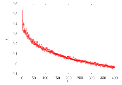
Figure 1: Partial Lyapunov spectrum from $512^{2}$ simulation, highlighting that the error is concentrated in a small number of the largest exponents.

A number of methods for computing the sampling error of correlated data have been developed for use in DNS hoyas ; oliver . They share a common feature in that they both make use of an extension of the central limit theorem to weakly dependant variables, see billingsley for details. We focus on the method detailed in oliver and use it to find the standard deviation in our measurments of the exponents, and thus the Kolmogorov-Sinai entropy. Importantly, this method lets us make use of all the possibly correlated samples we have and as such is an efficient use of our computational effort. For the case of the entropy, these errors are tabulated in Tables 1, 2 and 3. Also listed are the number of samples taken for each simulation.

In Fig. 1 we show a partial Lyapunov spectrum from a $512^{2}$ simulation. Here, it is clear that the largest exponents take the longest time to converge, as was reported in keefe1992dimension . For the lesser exponents, their error bars are smaller than the points themselves. Given that the Kolmogorov-Sinai entropy is determined by the sum of a large number of exponents, the influence of the largest exponents reuduced convergence is damped by the quick convergence of the remaining exponents. As such, the largest relative errors are found in cases with very few positive exponents.

IV Results

IV.1 Maximal Lyapunov exponent

As discussed in section II, depending on the form of the energy spectrum in the direct entrophy cascade region, there exist two possible scaling predictions for the maximal Lyapunov exponent, $\lambda_{1}$. The first of these predictions is valid if the energy spectrum takes the form $E(k)\sim k^{-3}$ and is given by Eq. 1, notably, this prediction has no Re dependence and is determined solely by the enstrophy dissipation rate, $\eta$. We note here that in our simulations, given the high computational demands imposed by the computation of a large number of Lyapunov exponents, we only achieve modest resolution. To illustrate this, in Fig. 2 we show the energy spectra from the highest resolution simulation in our data-set. It is clear that the spectrum in the enstrophy cascade region is steeper than $k^{-3}$. This is not surprising given the resolution achieved, and has been observed in previous studies legras ; Ohkitani91 . In Fig. 3 we show $\lambda_{1}$ against $\eta$ and we find our data is well fit by a power law of the form $\lambda_{1}=\alpha\eta^{1/3}$, with $\alpha=0.42\pm 0.01$. The calculation of the maximal exponent only requires the simultaneous integration of two velocity fields and is much less resource intesive when compared to the calculation of the entropy and attractor dimension. As such, by computing the maximal exponent in separate simulations, the number of samples is far larger, $N_{s}\approx 5,000$ in all cases, leading to small error.

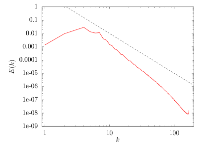
Figure 2: Energy spectrum from a $512^{2}$ simulation with $k_{f}=7$ and $k_{\mathrm{min}}=1$. Dashed line shows $k^{-3}$ scaling.

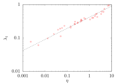
Figure 3: Plot of the enstrophy dissipation rate, $\eta$, against the largest Lyapunov exponent, $\lambda_{1}$. Dashed line shows the fit $0.42\eta^{1/3}$.

It was suggested by Kraichnan kraich71 that in order for the enstrophy flux to be constant in the direct cascade inertial range, then there should be a logarithmic correction to the energy spectrum. This alters the scaling prediction of Eq. 1 to that of Eq. 4 and introduces a dependence on Re. To test this we plot in Fig. 4 the product $\lambda_{1}\tau$, which, if Eq. 1 is correct, should be constant for all Re, against the Reynolds number. In doing so, we find $\lambda_{1}\tau$ slowly increases with $Re$, with the data being well fit by a power law of the form $\lambda_{1}\tau=\beta\mathrm{Re}^{\gamma}$, where $\beta=0.16\pm 0.02$ and $\gamma=0.16\pm 0.02$. Due to the the difficulties in accurate measurement, we choose not to test the logarithmic scaling with $Re$ predicted in Eq. 4, however, Fig. 4 does demonstrate that the maximal exponent does have a weak dependence on the Reynolds number. This weak dependence is in line with the logarithmic correction to the energy spectrum suggested by Kraichnan.

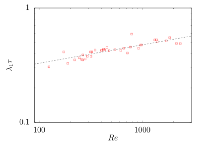
Figure 4: Plot of Re against the largest Lyapunov exponent multiplied by the enstrophy dissipation time $\eta^{-1/3}$. Dashed line shows a power law fit with $0.16\mathrm{Re}^{0.16}$.

IV.2 Kolmogorov-Sinai entropy

We turn now to the KS entropy for forced two dimensional turbulence. Once again, in Sec. II we presented two scaling predictions derived via dimensional arguments. The first Eq. 2 is derived for the case where there are no logarithmic corrections to the energy spectrum, whilst Eq. 5 is valid with these corrections. Both cases have a dependence on the enstrophy dissipation time and the Reynolds number, with the corrected prediction introducing an additional logarithmic dependence on Re. Due to the cost of computing the KS entropy scaling quickly with Re (see berera2019info for the three dimensional case which is more severe but illustrative), our results likely will not be able to quantify this logarithmic dependence, so we will focus on the prediction of Eq. 1.

Upon testing the prediction of Eq. 2 against our data we find there is no scaling behavior and the value of $h_{\mathrm{KS}}\tau$ varies by orders of magnitude for the same value of Re. Within this data-set there are a range of different values used for the forcing length scale $k_{f}$, as well as three different physical box side lengths. If we fix the box side length at $2\pi$, we find what has the appearance of three separate close to parallel lines, one corresponding to each value of $k_{f}$. This shows there is some form of scaling with the integral scale Reynolds number, but that this is not the full picture. In grappin1987computation the dimension of the attractor in two dimensional HIT was found to be dependent on $k_{f}$, however the exact dependence was not investigated. As such, the fact that our results for the entropy also show a $k_{f}$ dependence is not overly surprising, despite being at odds with Eq. 2.

In order to correct the prediction in Eq. 2 to account for this forcing scale dependence, we will consider what was found in grappin1991lyapunov , where it was observed that the attractor dimension grew at the same rate as the number of modes in the inverse energy cascade inertial range. Using this a reasonable ansatz for the correction factor, $C$, is

$$C\sim\left(\frac{k_{f}}{k_{\mathrm{min}}}\right)^{2},$$ (18)

where $k_{\mathrm{min}}$ is determined by the side length, $x$, of the box our fluid resides within using

$$k_{\mathrm{min}}=\frac{2\pi}{x}.$$ (19)

The typical choice in simulations is $x=2\pi$ restricting the allowed wavenumbers to integer values. By choosing $x=\pi$ and $x=\pi/2$ we have $k_{\mathrm{min}}=2$ and $k_{\mathrm{min}}=4$ respectively. Since energy is injected at $k_{f}$, then a natural lower bound for the inverse cascade is $k_{\mathrm{min}}$, and thus $C$ has the desired scaling behavior. We then consider a corrected scaling prediction for the KS entropy of the form

$$h_{\mathrm{KS}}\tau\left(\frac{k_{\mathrm{min}}}{k_{f}}\right)^{2}\sim\mathrm{Re}.$$ (20)

Using this new scaling prediction, our data is shown in Fig. 5. It can be seen that all points fall on a straight line, thus indicating a power law scaling. We find the data is well fit by a power law of the form $h_{\mathrm{KS}}\tau\left({k_{\mathrm{min}}}/k_{f}\right)^{2}=a\mathrm{Re}^{b}$, with $a=0.0018\pm 0.0005$ and $b=0.9\pm 0.03$. There is a notable spread in this data which we do not believe to be solely the result of sampling errors, which are reasonably small in general. Instead, this spread is likely explained by the use of the correction factor $C$ defined in Eq. 18. This factor does not contain any information regarding the structure of the underlying flow and is merely a ratio of length scales. However, without the use of such a term, no scaling at all is found for simulations with differing $k_{f}$ and $k_{min}$ values. It is likely a more flow specific correction can be found, but we do not pursue that here.

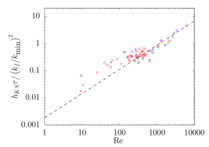
Figure 5: Plot of Re against the Kolmogorov-Sinai entropy $h_{\mathrm{KS}}$ scaled by the enstrophy dissipation time-scale and the ratio of $k_{f}$ to $k_{\mathrm{min}}$, fit corresponds to 0.0018Re^0.9. The values of ($k_{\mathrm{min}}$,$k_{f}$) are varied and displayed as $(1,3)$ red ($\times$), $(1,5)$ red ($\square$), $(1,7)$ red ($\circ$), $(1,9)$ red ($\bigtriangleup$), $(1,11)$ red ($\bigtriangledown$), $(2,4)$ blue ($\Diamond$), $(2,6)$ blue ($\pentagon$), $(4,8)$ black ($\square$) and $(4,12)$ black ($\circ$).

We now turn our attention to the scaling prediction given in Eq. 7. It is interesting that this prediction must also be corrected by $C$, or else the same issue of different scaling behaviors for each value of $k_{f}$ and $k_{\mathrm{min}}$ appears once more. We show this in Fig. 6 in which we have non-dimensionalized the entropy using $\sqrt{\nu/\varepsilon}$. The spread in the data here is more pronounced than for the simpler scaling of Eq. III; once more this is a combination of small sampling errors and the use of the correction factor $C$, the effect may be exacerbated in this case by the logarithmic scale and small values on the y-axis.

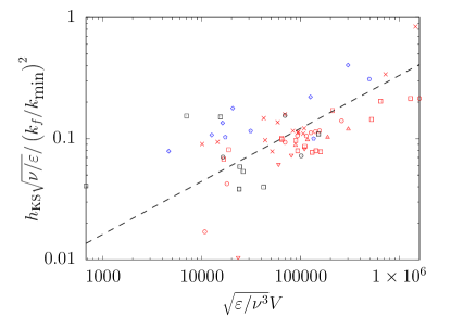
Figure 6: Plot of the scaling prediction for the Kolmogorov-Sinai entropy given by Ruelle and Lieb. The values of ($k_{\mathrm{min}}$,$k_{f}$) are varied and displayed as $(1,3)$ red ($\times$), $(1,5)$ red ($\square$), $(1,7)$ red ($\circ$), $(1,9)$ red ($\bigtriangleup$), $(1,11)$ red ($\bigtriangledown$), $(2,4)$ blue ($\Diamond$), $(2,6)$ blue ($\pentagon$), $(4,8)$ black ($\square$) and $(4,12)$ black ($\circ$).

Our data thus shows that the scaling of the Kolmogorov-Sinai entropy for two dimensional turbulence exhibits a dependence on both the forcing length scale and the system size. This is very much at odds with the picture in three dimensional turbulence, where we found the the scaling of the entropy is very close to that predicted in the K41 theory, depending only on small scale features of the flow berera2019info . This is perhaps best explained by considering the nature of the triadic interactions in two dimensional turbulence. In triad , it was shown that non-local triad interactions have an important effect on both the energy and enstrophy inertial ranges. When viewed in physical space this manifests itself in the appearance of long-lived coherent vortices, which then influence the small scales. As such, the fact that in two dimensions the large scales have a direct effect on the chaotic properties of the flow should not come as a surprise.

IV.3 Attractor dimension

By computing a large enough subset of the Lyapunov spectrum, it is also possible to make an estimate of the dimension of the attractor for forced two dimensional HIT. To do so, we make use of the Kaplan-Yorke conjecture kaplan1979chaotic , which suggests the attractor dimension can be found using

$$\mathrm{dim}(A)=j+\frac{\sum_{i=0}^{j}\lambda_{i}}{|\lambda_{j+1}|},$$ (21)

in which $j$ is the index of the Lyapunov exponent such that

$$\sum_{i=0}^{j}\lambda_{i}\geq 0,\quad\mbox{and}\quad\sum_{i=0}^{j+1}\lambda_{i}<0.$$ (22)

From this definition, it is clear that the computation of the attractor dimension will require more exponents than needed for the Kolmogorov-Sinai entropy. This definition makes quantifying the effect of the error in the Lyapunov exponents on the attractor dimension difficult. Any fluctuation in values of the exponents will effect the value of $j$ in a complex manner. As such, we do not include the standard deviation of the attractor dimension in either Table 1, 2 or 3, but it is likely to be of the order of the error in the Kolmogorov-Sinai entropy as both quantities are derived from the same data.

Naturally, the numerical computation of the attractor dimension comes at a severe computational cost. However, as with the entropy, when compared to the three dimensional case, the calculation for the attractor dimension is more favorable and a reasonable measurement of the scaling behavior can be made. The results of this measurement are displayed in Fig. 7 in which we have plotted against Re the scaling prediction of Eq. 2 corrected by the scaling factor $C$ described previously. Upon doing so, we find the data is well fit by a power law of the form $\mathrm{dim}(A)\left({k_{\mathrm{min}}}/k_{f}\right)^{2}=c\mathrm{Re}^{d}$ with $c=0.055\pm 0.02$ and $d=0.78\pm 0.04$. As with the entropy, we also find that when considering the Ruelle-Lieb prediction of Eq. 8, the correction factor is once again necessary and this is demonstrated in Fig. 8. Although the scatter is less in these figures, it is still present. This is again a result of a combination of sampling error and the use of the corrective term $C$. Notably, it is clear that data points with either low Re or higher $k_{\mathrm{min}}$, which have the fewest postive exponents, show the largest spead.

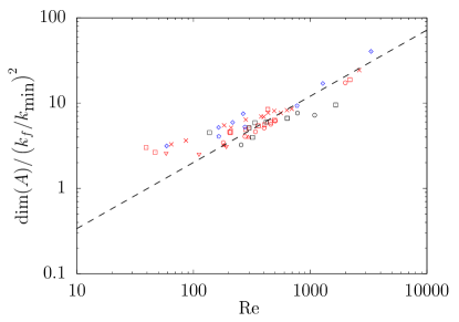
Figure 7: Plot of Re against the attractor dimension, $\mathrm{dim}(A)$ scaled by the ratio of $k_{f}$ to $k_{\mathrm{min}}$, fit corresponds to 0.055Re^0.78. The values of ($k_{\mathrm{min}}$,$k_{f}$) are varied and displayed as $(1,3)$ red ($\times$), $(1,5)$ red ($\square$), $(1,7)$ red ($\circ$), $(1,9)$ red ($\bigtriangleup$), $(1,11)$ red ($\bigtriangledown$), $(2,4)$ blue ($\Diamond$), $(2,6)$ blue ($\pentagon$), $(4,8)$ black ($\square$) and $(4,12)$ black ($\circ$).

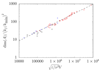
Figure 8: Plot of the attractor dimension scaling prediction given by Ruelle and Lieb. The values of ($k_{\mathrm{min}}$,$k_{f}$) are varied and displayed as $(1,3)$ red ($\times$), $(1,5)$ red ($\square$), $(1,7)$ red ($\circ$), $(1,9)$ red ($\bigtriangleup$), $(1,11)$ red ($\bigtriangledown$), $(2,4)$ blue ($\Diamond$), $(2,6)$ blue ($\pentagon$), $(4,8)$ black ($\square$) and $(4,12)$ black ($\circ$).

.

The attractor dimension gives a measure of the total number of active degrees of freedom in the flow. In grappin1991lyapunov , the attractor dimension was found to grow with the width of the energy inertial range. Our results are in agreement with this finding, although we also find a contribution from the enstrophy inertial range due to the dependence on the ratio of large to small scales in the flow measured by Re.

IV.4 Lyapunov spectrum

It is also of interest to investigate the shape of the Lyapunov spectrum, in particular, the distribution of exponents about $\lambda\approx 0$. It was suggested by Ruelle ruelle1982large ; ruelle1983five that it may be possible for the distribution of exponents to become singular about this point. Using the GOY shell model yamada1987lyapunov ; yamada1988lyapunov it was found that in both two and three dimensions the distribution of exponents did indeed become singular. However, it was later suggested that this divergence was caused by the numerical discretization employed in these works yamada1998asymptotic .

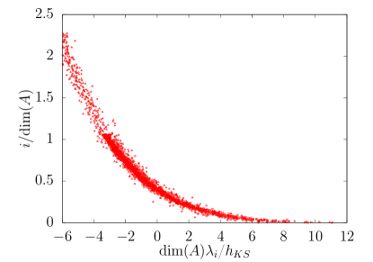
Figure 9: Lyapunov spectra normalized by $h_{KS}$ and dim$(A)$. The results of a number of simulations are shown here to highlight the similarity property of the spectra.

In Fig. 9, we show the Lyapunov spectra from a number of our simulations scaled by both their Kolmogorov-Sinai entropies and the attractor dimensions, such that the spectra collapse onto a single curve. From this figure, it is clear there is no divergence around $\lambda\approx 0$ in our simulations. This is consistent with what was found in three dimensional turbulence keefe1992dimension ; berera2019info ; spec , although it should be noted that in spec a ‘knee’-like structure was found around $\lambda\approx 0$, which is also seen in simulations of Rayleigh-Bénard convection xu . This structure does not, however, appear to be a true divergence.

V Conclusion

This work has been focused on the calculation of a number of standard measures of chaos in two dimensional forced incompressible HIT using pseudospectral DNS. A number of scaling predictions for these quantities have been made in the literature and, using our numerical results, we have tested a subset of them. It was found that the maximal exponent displays a weak dependence on the Reynolds number of the flow, consistent with the logarithmic correction to the energy spectrum suggested by Kraichnan. However, it was seen that for the Kolmogorov-Sinai entropy and attractor dimension, the predictions made on dimensional arguments were not sufficient. Corrections relating to the forcing length scale and system size were then found to be required. It is suggested that these corrections are required due to non-local effects in two dimensional turbulence as a result of coherent vortices.

When comparing these results to three dimensional turbulence, it is found that these chaotic properties scale with Re far more slowly in two dimensional turbulence. Futhermore, since these chaotic properties depend on large scale details of the flow in two dimensions, as opposed to only on small scale features in three dimensions, they provide further evidence of non-universality danilov in two dimensional turbulence. Given the two dimensional phenomenology seen in the atmospheres of the Earth and Jupiter nastrom ; young , this may have important implications for atmospheric predictability. In reality, this two dimensional phenomenology is not the entire story, as such systems are likely more accurately described by thin layer turbulence benav ; split . In thin layer turbulence, it is found that there are a number of critical points where the system transitions from purely three dimensional behavior to coexisting two and three dimensional phenomenology, and then from this state to purely two dimensional turbulence benav . It is in fact not just thin layer systems in which this kind of behavior is seen. Indeed, in systems undergoing rotation, as well as stratification and influence from an external magnetic field, a similar transition from three dimensional to two dimensional behavior is seen smith ; sozza ; alexak . The predictability of such would be of interest to study and compare with the idealized cases of pure HIT in two and three dimensions.

Such is the complexity of atmospheric systems, that even all of the variants discussed above only begin to scratch the surface. As such, simplified models which approximate the true dynamics of the atmosphere are often used. These models also exhibit sensitivity to initial conditions and, in some cases, Lyapunov spectra have been measured atmos . In one such case in a coupled atmosphere-ocean model atmos1 , a large number of near zero Lyapunov exponents are found, suggesting a possible divergence in the spectra. Whether this divergence is simply a feature of the simplified model or of the true dynamics is an interesting question, however, given the computation cost of even the simple case studied in this work, its answer is likely some way off.

- (1) E. Ott, Chaos in dynamical systems (Cambridge University Press, 2002).
- (2) T. Bohr, M. H. Jensen, G. Paladin, and A. Vulpiani, Dynamical systems approach to turbulence (Cambridge University Press, 2005).
- (3) E. N. Lorenz, Deterministic nonperiodic flow, J. Atmos. Sci. 20, 130 (1963).
- (4) D. Ruelle and F. Takens, On the nature of turbulence, Commun. Math. Phys. 20, 167 (1971).
- (5) G. K. Batchelor, The theory of homogeneous turbulence (Cambridge University Press, 1953).
- (6) C. E. Leith, Atmospheric predictability and two dimensional turbulence, J. Atmos. Sci. 28, 145 (1971).
- (7) C. E. Leith and R. H. Kraichnan, Predictability of turbulent flows, J. Atmos. Sci. 29, 1041 (1972).
- (8) A. N. Kolmogorov, The local structure of turbulence in incompressible viscous fluid for very large Reynolds numbers, Cr Acad. Sci. URSS 30, 301 (1941).
- (9) U. Frisch, Turbulence: The Legacy of A. N. Kolmogorov (Cambridge university press, 1995)
- (10) S. Kida, M. Yamada, and K. Ohkitani, Error growth in a decaying two-dimensional turbulence, J. Phys. Soc. Japan 59, 90 (1990).
- (11) G. Boffetta and S. Musacchio, Predictability of the inverse energy cascade in 2D turbulence, Phys. Fluids 13, 1060 (2001).
- (12) S. Kida and K. Ohkitani, Spatiotemporal intermittency and instability of a forced turbulence, Phys. Fluids A 4, 1018 (1992).
- (13) A. Berera and R. D. J. G. Ho, Chaotic properties of a turbulent isotropic fluid, Phys. Rev. Lett. 120, 024101 (2018).
- (14) G. Boffetta and S. Musacchio, Chaos and predictability of homogeneous-isotropic turbulence, Phys. Rev. Lett. 119, 054102 (2017).
- (15) P. Mohan, N. Fitzsimmons, and R. D. Moser, Scaling of Lyapunov exponents in homogeneous isotropic turbulence, Phys. Rev. Fluids 2, 114606 (2017).
- (16) R. D. J. G. Ho, A. Berera, and D. Clark, Chaotic behavior of Eulerian magnetohydrodynamic turbulence, Phys. Plasmas 26, 042303 (2019).
- (17) D. Ruelle, Microscopic fluctuations and turbulence, Phys. Lett. A 72, 81 (1979).
- (18) R. Benzi, G. Paladin, G. Parisi, and A. Vulpiani, On the multifractal nature of fully developed turbulence and chaotic systems, J. Phys. A 17, 3521 (1984).
- (19) A. Crisanti, M. H. Jensen, G. Paladin, and A. Vulpiani, Predictability of velocity and temperature fields in intermittent turbulence, J. Phys. A 26, 6943 (1993).
- (20) R. Grappin, J. Leorat, and A. Pouquet, Computation of the dimension of a model of fully developed turbulence, J. Phys. (Paris) 47, 1127 (1986).
- (21) M. Yamada and K. Ohkitani, Lyapunov spectrum of a chaotic model of three-dimensional turbulence, J. Phys. Soc. Jpn. 56, 4210 (1987).
- (22) M. Yamada and K. Ohkitani, Lyapunov spectrum of a model of two-dimensional turbulence, Phys. Rev. Lett. 60, 983 (1988).
- (23) R. Grappin and J. Leorat, Computation of the dimension of two-dimensional turbulence, Phys. Rev. Lett. 59, 1100 (1987).
- (24) R. Grappin and J. Leorat, Lyapunov exponents and the dimension of periodic incompressible Navier—Stokes flows: numerical measurements,J. Fluid Mech. 222, 61 (1991).
- (25) L. Keefe, P. Moin, and J. Kim, The dimension of attractors underlying periodic turbulent Poiseuille flow, J. Fluid Mech. 242, 1 (1992).
- (26) L. Van Veen, S. Kida, and G. Kawahara, Periodic motion representing isotropic turbulence, Fluid Dyn. Res. 38, 19 (2006).
- (27) A. Berera and D. Clark, Information production in homogeneous isotropic turbulence, Phys. Rev. E 100, 041101(R) (2019).
- (28) H. Xia, D. Byrne, G. Falkovich and M. Shats, Upscale energy transfer in thick turbulent fluid layers, Nat. Phys. 7, 321 (2011).
- (29) G. Nastrom, K. Gage and W. Jasperson, Kinetic energy spectrum of large-and mesoscale atmospheric processes, Nature 310, 36–38 (1984).
- (30) R. Young, P. Read, Forward and inverse kinetic energy cascades in Jupiter’s turbulent weather layer, Nat. Phys. 13, 1135–1140 (2017).
- (31) R. H. Kraichnan, Inertial ranges in two‐dimensional turbulence, Phys. Fluids 10, 1417–1423 (1967).
- (32) C. E. Leith, Diffusion approximation for two‐dimensional turbulence, Phys. Fluids 11, 671–673 (1968).
- (33) G. K. Batchelor, Computation of the energy spectrum in homogeneous two‐dimensional turbulence, Phys. Fluids Suppl. 12 (II), 233–239 (1969).
- (34) R. Shaw, Strange attractors, chaotic behavior, and information flow, Z. Naturforsch. Teil A 36(1), 80-112 (1981).
- (35) X. J. Wang and P. Gaspard, entropy for a time series of thermal turbulence, Phys. Rev. A 46, R3000 (1992).
- (36) R. H. Kraichnan, Inertial-range transfer in two-and three-dimensional turbulence, J. Fluid Mech. 47, 525 (1971).
- (37) K. Ohkitani, Log‐corrected energy spectrum and dimension of attractor in two‐dimensional turbulence, Phys. Fluids A 1, 451 (1989).
- (38) P. Constantin, C. Foias, and R. Temam, On the dimension of the attractors in two-dimensional turbulence, Physica (Amsterdam) 30D, 284 (1988)
- (39) D. Ruelle, Large volume limit of the distribution of characteristic exponents in turbulence, Commun. Math. Phys. 87, 287 (1982).
- (40) E. H. Lieb, On characteristic exponents in turbulence, Commun. Math. Phys. 92(4), 473-480 (1984).
- (41) R. Ho, et al., EddyBurgh code documentation (2018).
- (42) S. R. Yoffe, Investigation of the transfer and dissipation of energy in isotropic turbulence, Ph.D. thesis, University of Edinburgh, 2012, arXiv:1306.3408.
- (43) G. Boffetta and R. E. Ecke, Two-dimensional turbulence, Annu. Rev. Fluid Mech. 44, 427 (2012).
- (44) P. A. Davidson, Turbulence: An Introduction for Scientists and Engineers (Oxford University Press, New York, 2015)
- (45) G. Benettin, L. Galgani, A. Giorgilli, and J. Strelcyn, Lyapunov characteristic exponents for smooth dynamical systems and for Hamiltonian systems; a method for computing all of them. Part 1: Theory, Meccanica 15, 9 (1980).
- (46) L. Sirovich, and A. E. Deane, 1991. A computational study of Rayleigh-Bénard convection. Part 2. Dimension considerations. J. Fluid Mech. 222, 251-265 (1991).
- (47) S. Hoyas and J. Jiménez, Reynolds number effects on the Reynolds-stress budgets in turbulent channels, Phys. FLuids, 20(10), 101511 (2008).
- (48) T. A. Oliver, N. Malaya, R .Ulerich and R. D. Moser, Estimating uncertainties in statistics computed from direct numerical simulation, Phys. Fluids 26, 035101 (2014).
- (49) P. Billingsley, Probability and measure (John Wiley & Sons, 2008).
- (50) B. Legras, P. Santangelo, and R. Benzi, High-resolution numerical experiments for forced two-dimensional turbulence, Europhys. Lett. 5, 37 (1988)
- (51) K. Ohkitani, Wave number space dynamics of enstrophy cascade in a forced two‐dimensional turbulence, Phys. Fluids A3, 1598 (1991).
- (52) J. L. Kaplan and J. A. Yorke, in Functional Differential equations and approximation of fixed points (Springer, 1979) pp. 204–227.
- (53) M. E. Maltrud, G. K. Vallis, Energy and enstrophy transfer in numerical simulations of two‐dimensional turbulence, Phys. Fluids A 5 1760 (1993).
- (54) D. Ruelle, Five turbulent problems, Physica D 7, 40 (1983).
- (55) M. Yamada and K. Ohkitani, Asymptotic formulas for the Lyapunov spectrum of fully developed shell model turbulence, Phys. Rev. E 57, R6257 (1998).
- (56) M. Hassanaly and V. Raman, Lyapunov spectrum of forced homogeneous isotropic turbulent flows, Phys. Rev. Fluids 4, 114608 (2019).
- (57) M. Xu and M. R. Paul, Covariant Lyapunov vectors of chaotic Rayleigh-Bénard convection, Phys. Rev. E 93, 062208 (2016).
- (58) S. D. Danilov and D. Gurarie, Quasi-two-dimensional turbulence, Usp. Fiz. Nauk, 43(9), 863 (2000).
- (59) S.J. Benavides and A. Alexakis, Critical transitions in thin layer turbulence, J. Fluid Mech. 822, 364 (2017).
- (60) S. Musacchio and G. Boffetta, Split energy cascade in turbulent thin fluid layers, Phys. Fluids, 29(11), 111106 (2017).
- (61) L. M. Smith, J. R. Chasnov and F. Waleffe, Crossover from two-to three-dimensional turbulence, Phys. Rev. Lett. 77(12), 2467 (1996).
- (62) A. Sozza, G. Boffetta, P. Muratore-Ginanneschi and S. Musacchio, Dimensional transition of energy cascades in stably stratified forced thin fluid layers, Phys. Fluids 27(3), 035112 (2015).
- (63) K. Seshasayanan, and A. Alexakis, Critical behavior in the inverse to forward energy transition in two-dimensional magnetohydrodynamic flow, Phys. Rev. E 93(1), 013104 (2016)
- (64) S. Vannitsem, Predictability of large-scale atmospheric motions: Lyapunov exponents and error dynamics, Chaos 27(3), 032101 (2017).
- (65) S. Vannitsem and V. Lucarini, Statistical and dynamical properties of covariant lyapunov vectors in a coupled atmosphere-ocean model—multiscale effects, geometric degeneracy, and error dynamics, J. of Phys. A, 49(22), 224001 (2016).
- (66) Cirrus, http://www.cirrus.ac.uk.