Hydrodynamic limit for a 2D interlaced particle process

Abstract.

The Markov dynamics of interlaced particle arrays, introduced by A. Borodin and P. Ferrari in [3], is a classical example of $(2+1)$-dimensional random growth model belonging to the so-called Anisotropic KPZ universality class. In [9], a hydrodynamic limit – the convergence of the height profile, after space/time rescaling, to the solution of a deterministic Hamilton-Jacobi PDE with non-convex Hamiltonian – was proven when either the initial profile is convex, or for small times, before the solution develops shocks. In the present work, we give a simpler proof, that works for all times and for all initial profiles for which the limit equation makes sense. In particular, the convexity assumption is dropped. The main new idea is a new viewpoint about "finite speed of propagation" that allows to bypass the need of a-priori control of the interface gradients, or equivalently of inter-particle distances.

1. Introduction

In this work, we study a $(2+1)$-dimensional stochastic growth model, or equivalently an irreversible Markov process for a two-dimensional system of interlaced particles which perform totally asymmetric, unbounded jumps. This model was originally introduced by A. Borodin and P. Ferrari in [3] (we will refer to it as Borodin-Ferrari dynamics) together with a larger class of growth models that belong to the so-called Anisotropic KPZ universality class [18]; we refer to [9, 16, 3] for a discussion of this topic and for further references. Our focus here is not on interface fluctuations but on the hydrodynamic limit (i.e. the law of large numbers for the height profile $H(x,t)$). For models in the AKPZ class, the rescaled height profile is conjectured to converge to the viscosity solution of a non-linear Hamilton-Jacobi PDE [2]

$$\partial_{t}u+v(\nabla u)=0,$$ (1.1)

with non-convex Hamiltonian $v$. In fact, the feature that distinguishes the AKPZ class from the usual KPZ class is that the Hessian $D^{2}v$ has negative determinant [18]. The absence of convexity has an important consequence on the hydrodynamic behavior. First of all, there is no Hopf-Lax formula for the solution of (1.1). Moreover, there is no hope that the subadditivity arguments developed in [14, 13] apply, since they would automatically yield a convex Hamiltonian. Let us recall that the methods of [14, 13] require (at the microscopic level) the so-called “envelope property”, which is a strong version of monotonicity and which gives a microscopic analog of Hopf-Lax formula. For AKPZ models, the envelope property simply fails to hold.

In the previous work [9], the convergence (in probability) of the height profile to the viscosity solution of (1.1) was proven, under the important restriction that either the initial profile $u_{0}$ is convex, or that time is smaller than the time when shocks (discontinuities of $\nabla u$) appear. In the present article, instead, we prove the result for all initial profiles and for all times (and convergence holds almost surely). Our proof is strongly inspired by the method developed by F. Rezakhanlou in [12]; in few words, it consists in showing that the Markov semigroup that encodes the dynamics is tight in a certain topology and that all of its limit points satisfy a set of properties that are sufficient to identify them with the unique semi-group associated to the PDE (1.1). These ideas have been recently employed in [19, 10] to obtain a full hydrodynamic limit for other $(2+1)$-dimensional growth models in the AKPZ class, namely the “domino shuffling algorithm” and the Gates-Westcott model [11]. The reason why Rezakhanlou’s method was not employed in [9] is that it requires a strong (i.e. uniform with respect to the initial condition) form of locality or of “finite speed of propagation” for the dynamics. Such property is easy to check for the “domino shuffling” or the Gates-Westcott dynamic, but it fails for the Borodin-Ferrari dynamics. The reason for this is that particle jumps are not bounded; the larger the typical inter-particle distance in the initial condition, the faster information propagates through the system.

The main new idea of the present work, that allows to overcome the limitations of [9], is the following. The usual locality property would say that the height function $H(x,t)$, for fixed $x$ and $t\leq T$, is with high probability not influenced (for $T$ large and uniformly in the initial condition) by the value of the initial profile $H(\cdot,0)$ outside a ball of radius $O(T)$ centered at $x$. This fails for the Borodin-Ferrari dynamics: locality holds but not uniformly, due to the lack of any a-priori control of typical inter-particle distances at times $t>0$. In contrast, our Proposition 3.5 shows that the height $H(x,t)$ is entirely determined by the height $H$ on a certain deterministic, compact subset of space-time, depending on $(x,t)$ but independent of the initial condition. As explained in Section 3.2, underlying this property is a bijection between the Borodin-Ferrari dynamics and a discretized version of the Gates-Westcott growth model. This bijection is the analogue of the well-known mapping between the Hammersley process and the Polynuclear growh (PNG) growth model [7].

As a side remark, with respect to the method of [12], we avoid studying directly the convergence of the Markov semi-group; this streamlines somewhat the argument.

Organization of the article. This work is organized as follows. The model and its height function are defined in Section 2.1 and 2.2, while the main theorem is given in Section 2.4. Section 3 proves a few general properties of the process, including the new locality statement. Compactness of sequences of rescaled height profiles is proven in Section 4 and the identification of limit points with the solution of the PDE is obtained in Section 5.

2. The model and the main result

2.1. The Borodin-Ferrari dynamics

We start by recalling the definition of the Borodin-Ferrari dynamics, as a Markov evolution of a two-dimensional array of interlaced particles. In the original reference [3], particles perform jumps of length 1 to the right and can “push” a number $n\geq 0$ of other particles; we rather follow the equivalent representation used in [17, 9], where particles jump a distance $k\geq 1$ to the left, and no particles are pushed. The lattice where particles live consists of an infinite collection of discrete horizontal lines, labeled by an index $\ell\in\mathbb{Z}$. Each line contains an infinite collection of particles, each with a label $(p,\ell)$, $p\in\mathbb{Z}$. See Figure 1. Horizontal particle positions $z_{(p,\ell)}$ are discrete:

$$z_{(p,\ell)}\in\mathbb{Z}+(\ell\!\!\!\!\mod 2)/2$$

(note that adjacent horizontal lines are displaced by a half interger).

Definition 1.

We let $\Omega$ be the set of particle configurations $\eta$ satisfying the following properties:

1. no two particles in the same line $\ell$ share the same position $z_{(p,\ell)}$. We label particles in each line in such a way that $z_{(p,\ell)}<z_{(p+1,\ell)}$. Labels are attached to particles, and they do not change along the dynamics.

2. particles are interlaced: for every $\ell$ and $p$, there exists a unique $p^{\prime}\in\mathbb{Z}$ such that $z_{(p,\ell)}<z_{(p^{\prime},\ell+1)}<z_{(p+1,\ell)}$ (and, as a consequence, also a unique $p^{\prime\prime}\in\mathbb{Z}$ such that $z_{(p,\ell)}<z_{(p^{\prime\prime},\ell-1)}<z_{(p+1,\ell)}$). Without loss of generality, we assume that $p^{\prime}=p$ (and therefore $p^{\prime\prime}=p+1$). This can always be achieved by deciding which particle is labeled $0$ on each line. Also, by convention, we establish that the particle labeled $(0,0)$ is the left-most one on line $\ell=0$, with non-negative horizontal coordinate.

3. for $\ell=0$ (and therefore for every $\ell$, because of the interlacement condition) one has

   $$\lim_{p\to-\infty}\frac{z_{(p,\ell)}}{p^{2}}=0.$$ (2.1)

Here we give an informal description of the dynamics; a rigorous (graphical) definition was given in [9, Sec. 2.3]. We will not recall the details of this construction here and we will use it only implicitly: we will work with the informal definition of the dynamics, and the existence of the graphical construction guarantees that the arguments are actually rigorous.

Given the particle label $(p,\ell)$, we denote $I_{(p,\ell)}=\{(p-1,\ell+1),(p,\ell-1)\}$, see Fig. 1: these are the labels of the two particles directly to the left of $(p,\ell)$ on lines $\ell+1$ and $\ell-1$.

Figure 1. The set $I_{(p,\ell)}$ comprises the particle labels of the two particles in the dotted region. The particle $(p,\ell)$ can jump to the position marked by the cross (and does so with rate $1$) but cannot jump to the position marked by a square.

To every pair $(\ell,z)$ with $\ell\in\mathbb{Z}$ and $z\in\mathbb{Z}+(\ell\!\!\mod 2)/2$ we associate an i.i.d. Poisson clock of rate $1$ (we will denote $W$ the realization of all the Poisson processes). When the clock labeled $(\ell,z)$ rings, then:

• if position $(\ell,z)$ is occupied, i.e. if there is a particle on line $\ell$ with horizontal position $z$, then nothing happens;

• if position $(\ell,z)$ is empty, let $(p,\ell)$ denote the label of the left-most particle on line $\ell$, with $z_{(p,\ell)}>z$. If both particles with label in $I_{(p,\ell)}$ have horizontal position smaller than $z$, then particle $(p,\ell)$ is moved to position $(\ell,z)$; otherwise, nothing happens.

In words: is position $(\ell,z)$ is empty, then particle $(p,\ell)$ is moved to position $(\ell,z)$ if and only if the new configuration is still in $\Omega$, i.e. if the interlacement constraints are still satisfied. Despite the fact that particle jumps are unbounded, the dynamics is well defined for almost every realization $W$ of the Poisson clocks, thanks to the condition (2.1) on particle spacings. A proof via the graphical representation is given in [9].

As observed in [9, Remark 2.2], the evolution of the particles on each line $\ell$ follows the one-dimensional (discrete) Hammersley-Aldous-Diaconis (HAD) process [6], except that particle jumps can be prevented by the interlacing constraints with particles in lines $\ell\pm 1$. This induces very strong correlations between the processes on different lines. As proven in [17], the translation invariant, stationary measures of the Borodin-Ferrari dynamics correspond (via the tiling-to-interlacing particle bijection recalled in Section 2.2.1) to the the translation invariant, ergodic Gibbs measures of rhombus tilings of the triangular lattice. In particular, the restriction of the stationary measures to any line $\ell$ is very different from the (i.i.d. Bernoulli) invariant measures of the HAD process: while for the latter the particle occupation variables are i.i.d., for the former they have power-law correlations.

2.2. Height function

To each configuration $\eta\in\Omega$ we associate an integer-valued height function $h_{\eta}$. The relation with the height function of rhombus tilings of the plane is recalled in Section 2.2.1.

The graph $G$ whose vertices are all the possible particle positions $(\ell,z),\ell\in\mathbb{Z},z\in\mathbb{Z}+(\ell\!\!\mod 2)/2$ and where the neighbors of $(\ell,z)$ are the four vertices $(\ell\pm 1,z\pm 1/2)$ can be identified with $\mathbb{Z}^{2}$, rotated by $\pi/4$ and suitably rescaled, see Figure 2. The height function $h_{\eta}$ is defined on the dual graph $G^{*}$, obtained by shifting $G$ horizontally by $1/2$, see Figure 2.

Figure 2. The lattice $G$ (dotted, with black vertices that are possible particle positions $(\ell,z)$, with $z\in\mathbb{Z}+(\ell\!\!\mod 2)/2$), the lattice $G^{*}$ (bold, with white vertices) and the two coordinate vectors $e_{1},e_{2}$. The origin of $G^{*}$ (encircled) is the point of horizontal coordinate $z=-1/2$ on line $\ell=0$.

We make the following choice of coordinates on $G^{*}$:

Definition 2 (Coordinates on $G^{*}$).

The point of $G^{*}$ of horizontal coordinate $-1/2$ of the line labeled $\ell=0$ is assigned the coordinates $(x_{1},x_{2})=(0,0)$. The unit vector $e_{1}$ (resp. $e_{2}$) is the vector from $(0,0)$ to the point of horizontal coordinate $0$ on the line labeled $\ell=-1$ (resp. $\ell=+1$), see Figure 2. With this convention, the vertex of $G^{*}$ labeled $(x_{1},x_{2})$ is on line

$$\bar{\ell}(x)=x_{2}-x_{1}$$ (2.2)

and has horizontal coordinate

$$\bar{z}(x)=(x_{1}+x_{2}-1)/2.$$ (2.3)

We can now define the height function $h_{\eta}$:

Definition 3 (Height function).

Given a configuration $\eta\in\Omega$, its height function $h_{\eta}$ is an integer-valued function defined on $G^{*}$. We fix $h_{\eta}(0,0)$ to any constant (for instance, zero). The gradients $h_{\eta}(x_{1}+1,x_{2})-h_{\eta}(x_{1},x_{2})$ and $h_{\eta}(x_{2},x_{2}+1)-h_{\eta}(x_{1},x_{2})$ are defined as follows. Given $(x_{1},x_{2})\in G^{*}$, let $p$ (resp. $p+1$) be the index of the rightmost (resp. leftmost) particle on line $\ell=x_{2}-x_{1}$ that is to the left (resp. to the right) of $(x_{1},x_{2})$. Recall that particle $p$ of line $\ell+1$ satisfies $z_{p,\ell}<z_{p,\ell+1}<z_{p+1,\ell}$. We establish that

$$\Delta_{2}h_{\eta}(x_{1},x_{2}):=h_{\eta}(x_{1},x_{2}+1)-h_{\eta}(x_{1},x_{2})\\ =\left\{\begin{array}[]{ccc}0&\text{if}&(x_{1},x_{2}+1)\text{ is to the right of particle }(p,\ell+1)\\ 1&\text{if}&(x_{1},x_{2}+1)\text{ is to the left of particle }(p,\ell+1)\end{array}\right.$$ (2.4)

and similarly

$$\Delta_{1}h_{\eta}(x_{1},x_{2}):=h_{\eta}(x_{1}+1,x_{2})-h_{\eta}(x_{1},x_{2})\\ =\left\{\begin{array}[]{ccc}0&\text{if}&(x_{1}+1,x_{2})\text{ is to the right of particle }(p+1,\ell-1)\\ 1&\text{if}&(x_{1}+1,x_{2})\text{ is to the left of particle }(p+1,\ell-1).\end{array}\right.$$ (2.5)

See Figure 3.

It is immediately checked that

$$\Delta_{1}h_{\eta}(x_{1},x_{2})+\Delta_{2}h_{\eta}(x_{1}+1,x_{2})=\Delta_{2}h_{\eta}(x_{1},x_{2})+\Delta_{1}h_{\eta}(x_{1},x_{2}+1)\\ =h_{\eta}(x_{1}+1,x_{2}+1)-h_{\eta}(x_{1},x_{2})\\ =\left\{\begin{array}[]{ll}0&\text{if $\exists$ particle between }(x_{1},x_{2})\text{ and }(x_{1}+1,x_{2}+1)\\ 1&\text{if $\nexists$ particle between }(x_{1},x_{2})\text{ and }(x_{1}+1,x_{2}+1).\end{array}\right.$$ (2.6)

The first equality in (2.6) implies that the sum of gradients of $h_{\eta}$ along any closed circuit is zero, so that the definition of $h_{\eta}$ is well-posed.

Figure 3. A portion of particle configuration and the corresponding height function. Particles (black dots) are on vertices of $G$ and the height is defined on vertices of $G^{*}$.

Let $\Gamma$ be the set of admissible height functions:

$$\Gamma:=\{h_{\eta},\>\eta\in\Omega\},$$ (2.7)

where it is understood that we allow the value $h_{\eta}(0)$ to be any integer. We also recall from [9] the definition

$$\Omega_{M}:=\{\eta\in\Omega,\>z_{(p,\ell)}-z_{(p-1,\ell)}\leq M\text{ for every }\ell,p\}$$ (2.8)

and we introduce the corresponding set of height functions

$$\Gamma_{M}:=\{h_{\eta},\>\eta\in\Omega_{M}\}.$$ (2.9)

Given an initial height function $h\in\Gamma$, the height at time $t$ is defined as

$$H(x,t)=h(x)-J_{x}(t),$$ (2.10)

where $J_{x}(t)\geq 0$ denotes the number of particles, on the line labelled $\bar{\ell}(x)=x_{2}-x_{1}$, that crossed (from right to left) the horizontal position $\bar{z}(x)=(x_{1}+x_{2}-1)/2$ in the time interval $[0,t]$.

To emphasize the dependence of $H$ on the initial height configuration $h$ and on the realization $W$ of the Poisson Point Process of intensity $1$ on $G\times\mathbb{R}_{+}$, we write more explicitly

$$H(x,t;h,W).$$

2.2.1. Height function and mapping to rhombus tilings

For a better intuition on the height function, let us recall that there is a bijection between interlaced particle configurations satisfying properties (1)-(2) of Definition 1 and rhombus tilings of the plane, as in Figure 4.

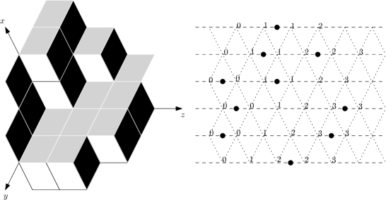
Figure 4. The bijection between rhombus tiling (or stepped interface) and particle configuration: vertical (black) rhombi correspond to particles (dots). It is easily checked that the height function in the right figure corresponds to the height in the $z$ direction, that is w.r.t. the $(x,y)$ plane, of the pile of cubes in the left figure.

Particles correspond to vertical rhombi: the vertical coordinate of the centre of a vertical rhombus defines the line the particle is on, and its horizontal coordinate corresponds to the $z_{(p,\ell)}$ coordinate of the particle. If lengths are rescaled in such a way that rhombi have sides of length $1$, then horizontal positions are shifted by half-integers between neighboring lines (as is the case for particles). It is well known (and easy to understand from the picture) that horizontal positions of rhombi in neighboring lines satisfy the same interlacing conditions as particle positions $z_{(p,\ell)}$, and that the tiling-to-particle configuration mapping is a bijection.

Given a rhombus tiling as in Figure 4 and viewing it as the boundary of a stacking of unit cubes in $\mathbb{R}^{3}$, a natural definition of height function is to assign to each vertex of a rhombus the height (i.e. the $z$ coordinate) w.r.t. the $(x,y)$ plane of the point (in $\mathbb{R}^{3}$) in the corresponding unit cube. As a consequence, height is integer-valued and defined on points that are horizontally shifted $1/2$ w.r.t. centers of rhombi, i.e. on points of $G^{*}$. The height function defined in the previous section equals the height of the stack of cubes w.r.t. the $(x,y)$ plane.

2.3. Slopes and speed

Here we define the set of continuous height functions that are possible scaling limits of the discrete height profile $H$, and the speed of growth function $v$ (or “Hamiltonian”) that appears in the limit PDE. Given an integer $M$, define $\bar{\Gamma}_{M}$ to be the set of functions $f:\mathbb{R}^{2}\rightarrow\mathbb{R}$ that are non-decreasing in both coordinates and such that

$$\frac{f(x+\lambda(1,1))-f(x)}{\lambda}\leq 1-\frac{1}{M}\text{ for every }x\in\mathbb{R}^{2},\,\lambda\in\mathbb{R}.$$

If $f$ is differentiable, this means that $\nabla f$ belongs to the triangle $\mathbb{T}_{M}$ defined by

$$\mathbb{T}_{M}:=\{\rho\in\mathbb{R}^{2}:\rho_{1},\rho_{2}\geq 0,\,\rho_{1}+\rho_{2}\leq 1-M^{-1}\}.$$ (2.11)

Define also

$$\bar{\Gamma}:=\bigcup_{M\in\mathbb{N}}\bar{\Gamma}_{M}\quad\text{and}\quad\mathbb{T}:=\{\rho\in\mathbb{R}^{2}:\rho_{1},\rho_{2}\geq 0,\,\rho_{1}+\rho_{2}<1\}=\bigcup_{M\in\mathbb{N}}\mathbb{T}_{M}.$$ (2.12)

We define the speed function $v(\cdot)$ as follows:

$$v(\rho)=\frac{1}{\pi}\frac{\sin(\pi\rho_{1})\sin(\pi\rho_{2})}{\sin(\pi(\rho_{1}+\rho_{2}))}\geq 0,\quad\rho\in\mathbb{T}$$ (2.13)

with the convention that $v(0)=0$. Note that $v(\cdot)$ vanishes if $\rho\in\mathbb{T}$ with $\min(\rho_{1},\rho_{2})=0$. Also, $v(\cdot)$ tends to $+\infty$ if $\rho\to(\bar{\rho}_{1},1-\bar{\rho}_{1})$ with $\bar{\rho}_{1}\in(0,1)$. On the other hand, $v(\cdot)$ does not admit a unique limit for $\rho\to(0,1)$ or $\rho\to(1,0)$ (any value in $[0,+\infty]$ can be obtained as limit point).

Remark 1.

The speed function $v$ is non-decreasing in both coordinates and is Lipschitz on every $\mathbb{T}_{M}$ since $\nabla v(\rho)=\left(\frac{\sin^{2}(\pi\rho_{2})}{\sin^{2}(\pi(\rho_{1}+\rho_{2}))},\frac{\sin^{2}(\pi\rho_{1})}{\sin^{2}(\pi(\rho_{1}+\rho_{2}))}\right)$ is bounded on $\mathbb{T}_{M}$. One can also check that the determinant of the Hessian of $v$ is negative (strictly negative in the interior of $\mathbb{T}$) and thus the model belongs to the AKPZ universality class [18].

2.4. The hydrodynamic limit

Theorem 2.1.

Given an integer $M$, let $f\in\bar{\Gamma}_{M}$ and let $(h_{L})_{L\in\mathbb{N}}\in\Gamma_{M}^{\mathbb{N}}$ be a sequence of height functions approaching $f$ in the following sense:

$$\forall R>0\qquad\sup_{\|x\|\leq R}\left|\frac{1}{L}h_{L}(\lfloor Lx\rfloor)-f(x)\right|\underset{L\to\infty}{\longrightarrow}0.$$ (2.14)

Then, for almost every realization $W$, the following hydrodynamic limit holds:

$$\forall T>0\quad\forall R>0\qquad\sup_{\|x\|\leq R,t\in[0,T]}\left|\frac{1}{L}H(\lfloor Lx\rfloor,Lt;h_{L},W)-u(x,t)\right|\underset{L\to\infty}{\longrightarrow}0\ ,$$ (2.15)

where $u$ is the unique viscosity solution of the Hamilton-Jacobi equation:

$$\left\{\begin{aligned} \partial_{t}u+{v}(\nabla u)&=0\\ u(\cdot,0)&=f.\end{aligned}\right.$$ (2.16)

Remark 2.

The condition $h_{L}\in\Gamma_{M}$ for some integer $M$ makes sure that the dynamics is well defined and satisfies the "finite speed of propagation" property (see Proposition 3.3); this condition could be somewhat weakened. On the other hand, the requirement that $f\in\bar{\Gamma}_{M_{0}}$ for some integer $M_{0}$ (we take for simplicity $M_{0}=M$) ensures that the slopes remain uniformly away from the the side $\rho_{1}+\rho_{2}=1$ of the triangle $\mathbb{T}$ where the speed $v$ is ill-defined. This condition is in a sense optimal: in fact, if $f$ is for instance the affine function of slope $\rho$ with $\rho_{1}+\rho_{2}=1$ and $h_{L}$ approaches $f$ as in (2.14), then the limit height profile will be either $+\infty$ for all positive times (if $\rho_{1}\in(0,1)$) or the limit is not necessarily unique (if $\rho_{1}\in\{0,1\}$), i.e. it may depend on the microscopic details of the initial condition $h_{L}$.

Remark 3.

As observed above, the function $v(\cdot)$ cannot be extented continuously to the whole boundary of $\mathbb{T}$, so Eq. (2.16) requires some care. What is really meant in the theorem is that $u$ is the unique viscosity solution of the PDE where $v(\cdot)$ is replaced by $\tilde{v}(\cdot)$, which is any Lipschitz extension of $v(\cdot)$ to the whole $\mathbb{R}^{2}$ that coincides with $v$ on $\mathbb{T}_{M}$. Since in this case the Hamiltonian is Lipschitz and depends only on the gradient, the standard theory of viscosity solutions implies that the solution $u$ exists and is unique, and the comparison principle shows that if $f\in\bar{\Gamma}_{M}$, then $u(\cdot,t)\in\bar{\Gamma}_{M}$ for all times, so that $u$ does not depend on the way $\tilde{v}$ is defined outside $\mathbb{T}_{M}$. For a reference on Hamilton-Jacobi equations, see e.g [2, Sections 5 and 7].

3. Properties of the microscopic dynamic

In this section, we recall some basic properties of the dynamics following [9]. In addition, we prove in Section 3.2 a new locality property that is crucial in the proof of Theorem 2.1.

3.1. Translation invariance, monotonicity and speed of propagation

We begin with a couple of easy facts:

Proposition 3.1.

The dynamics satisfies the following properties:

1. Vertical translation invariance: $H(x,t;h+c,W)=H(x,t;h,W)+c$ for all $c\in\mathbb{Z}$

2. Monotonicity: $h\leq h^{\prime}\Rightarrow H(x,t;h,W)\leq H(x,t;h^{\prime},W)$.

The former statement is trivial and the latter follows from [9, Th. 5.7].

Next, we recall a locality property established in [9] and we improve it to an almost sure statement (but the really new locality result will come in next section). Informally, Proposition 5.12 in [9] tells that if we fix a lattice site $x$ and an initial height function $h\in\Gamma_{M}$, then with probability $1-O(\exp(-c(M)n)$ the height function at $x$ up to time $n$ only depends on the Poisson clocks at positions within distance $\mathrm{O}(n)$ from $x$. Without much extra effort (we leave details to the reader), it is possible to show the following slightly stronger statement (the difference with respect to [9, Prop. 5.12] is that the claim (3.1) holds simultaneously for every $h\in\Gamma_{M}$):

Lemma 3.2.

Fix $x\in\mathbb{Z}^{2}$. For every integer $M$, there exist $c=c(M)>0$ and $\Delta=\Delta(M)>0$ such that for every integer $n$, for a set of realizations $W$ of probability $1-ce^{-n/c}$ of the Poisson process, the following happens for any $h\in\Gamma_{M}$:

$$H(x,t;h,W)=H(x,t;h,\tilde{W})\text{ for every }t\leq\Delta n,$$ (3.1)

for every $\tilde{W}$ that coincides with $W$ on

$$R_{n}(x):=B(x,2n)\times[0,\Delta n],$$

with $B(x,r)$ the ball of radius $r$ centered at $x$.

In the proof of Theorem 2.1, we need instead an almost sure result:

Proposition 3.3 (Finite speed of propagation).

For almost every $W$ the following holds: for every integer $M$ there exists $\alpha=\alpha(M)$ such that for every time $T>0$, every $x_{0}\in\mathbb{R}^{2}$ and every $R\geq 0$, we have for $L$ large enough

$$H(x,t;h,W)=H(x,t;h,\tilde{W})\text{ for every }t\leq LT,\,x\in B(Lx_{0},LR),\,h\in\Gamma_{M}$$ (3.2)

for every $\tilde{W}$ that coincides with $W$ on

$$B(Lx_{0},L(R+\alpha T))\times[0,LT].$$ (3.3)

Proof.

If we apply Lemma 3.2 with $n:=\lceil LT/\Delta\rceil$, use an union bound for all $x$ in $B(0,L^{2})$ (so that it includes all $x$ in $B(Lx_{0},LR)$ for any fixed $x_{0}\in\mathbb{R}^{2}$ and all $L$ large enough) and apply Borel-Cantelli Lemma, we get the following. For almost every $W$, every integer $M$, every rational $T>0$, every $x_{0}\in\mathbb{R}^{2}$ and every $R\geq 0$, (3.2) holds all $L$ large enough and for every $\tilde{W}$ that coincides with $W$ on the domain $B(Lx_{0},L(R+\alpha T))\times[0,LT]$ with $\alpha$ chosen large enough ($\alpha=2\Delta^{-1}$ suffices) such that this domain contains every $R_{\lceil LT/\Delta\rceil}(x)$ with $x\in B(Lx_{0},LR)$. The rest of the proof follows from rational approximation of $T$. ∎

Corollary 3.4 (Weak Locality).

For almost every $W$ the following holds: for every integer $M$ there exists $\alpha=\alpha(M)>0$ such that for every $T>0$, every $R\geq 0$, for $L$ large enough

$$\sup_{\begin{subarray}{c}x\in B(0,LR)\\ t\leq LT\end{subarray}}|H(x,t;h,W)-H(x,t;h^{\prime},W)|\leq\sup_{x\in B(0,L(R+\alpha T))}|h(x)-h^{\prime}(x)|$$ (3.4)

for every $h,h^{\prime}\in\Gamma_{M}$.

Proof.

We fix $W$ in the event of probability $1$ of Proposition 3.3. Let $M\in\mathbb{N},T>0,R\geq 0$ and let $h,h^{\prime}\in\Gamma_{M}$. We define $m$ as the supremum in the r.h.s of (3.4) and we set $h^{\prime\prime}:=h^{\prime}+m$. Since $h\leq h^{\prime\prime}$ on $B(0,L(R+\alpha T))$, the local version of monotonicity stated in [9, Theorem 5.10] implies that for all $L\geq 1$

$$H(x,t;h,\tilde{W})\leq H(x,t;h^{\prime\prime},\tilde{W})\text{ for every }x\in B(0,LR),\,t\leq LT$$

where $\tilde{W}$ is the restriction of $W$ to $B(0,L(R+\alpha T))\times[0,LT]$. By finite speed of propagation (Proposition 3.3) and by vertical translation invariance (Proposition 3.1), for all $L$ large enough, we have for all $t\leq LT$ and $x\in B(0,LR)$,

$$H(x,t;h,W) =H(x,t;h,\tilde{W})\leq H(x,t;h^{\prime\prime},\tilde{W})$$

$$=H(x,t;h^{\prime}+m,W)=H(x,t;h^{\prime},W)+m.$$

Similarly, we can show that for all $L$ large enough, for all $t\leq LT$ and $x\in B(0,LR)$, $H(x,t;h^{\prime},W)\leq H(x,t;h,W)+m,$ which concludes the proof of Corollary 3.4. ∎

We point out that the speed of propagation $\alpha(M)$ is not uniform in $M$. This is a problem, since later we would need to apply the propagation of information result from time $s>0$ to time $t>s$ but, while we know by construction that the initial condition belongs to $\Gamma_{M}$, the same does not hold at the later times $s>0$ (and we do not see how to obtain an apriori control on $M(s)$ such that $\eta(s)\in\Gamma_{M(s)}$). This is the main difficulty that prevented a proof of a full hydrodynamic limit in [9] and this is why we call a result like Corollary 3.4 “weak locality” (it is much weaker than the locality statements used e.g. in [10, 12, 19] to prove full hydrodynamic limits). One of the novelties of this article is a smarter locality property that we state and prove in the next section.

3.2. A new version of locality

In this section, we prove a very useful result of locality that says informally that if any height function $H$ is smaller than a height function $H^{\prime}$ in a specific bounded space-time domain, then we also have that $H(x,t)\leq H^{\prime}(x,t)$.

Let us start by introducing some notations. For any $\ell\in\mathbb{N}$, we note $T_{\ell}\subseteq\mathbb{Z}^{2}$ the following triangle of size $\ell$ (see Figure 5)

$$T_{\ell}=\{y=(y_{1},y_{2})\in\mathbb{Z}^{2},\>-2\ell<y_{1}\leq 0,\,-2\ell<y_{2}\leq 0,\,-2\ell\leq y_{1}+y_{2}\leq 0\}$$ (3.5)

and for all $t\geq 0$,

$$E_{\ell}=(0,0,-\ell)\cup\bigcup_{y\in T_{\ell}\setminus\{(0,0)\}}\{y\}\times[-\ell-\lfloor(y_{1}+y_{2})/2\rfloor-1,-\ell-\lfloor(y_{1}+y_{2})/2\rfloor]\subseteq\mathbb{Z}^{2}\times\mathbb{R}.$$ (3.6)

Finally, for $x\in\mathbb{Z}^{2}$ and $t\geq\ell$, we define the space-time translated set

$$E_{x,t,\ell}:=(x,t)+E_{\ell}\subseteq\mathbb{Z}^{2}\times\mathbb{R}_{+}.$$ (3.7)

Figure 5. The triangle $T_{\ell}$ for $\ell=5$.

Proposition 3.5 (Space-time locality).

Let $(x,t)\in\mathbb{Z}^{2}\times\mathbb{R}_{+}$ and $l\in\mathbb{N}$ such that $t\geq\ell$. Also, let $h,h^{\prime}\in\Gamma$. Then, we have

$$H(\cdot,\cdot;h,W)\leq H(\cdot,\cdot;h^{\prime},W)\text{ on }E_{x,t,\ell}\Rightarrow H(x,\cdot;h,W)\leq H(x,\cdot;h^{\prime},W)\text{ on }[t-\ell,t].$$ (3.8)

We emphasize that the main difference between a statement like Corollary 3.4 and Proposition 3.5 is that, while in both cases the difference between $H$ and $H^{\prime}$ at some $(x,t)$ is estimated in terms of the difference in some domain, in the former case the size of the domain depends on the bound $M$ on the inter-particle distances, while in the latter it is independent of it.

Before proving Proposition 3.5, let us explain briefly where it comes from. This is best understood in the easier case of the one-dimensional Hammersley (or Hammersley-Aldous-Diaconis) process [1], whose definition we recall informally. The state space consists of locally finite sets of points (or “particles”) that lie on $\mathbb{R}$. Particles jump to the left and jumps are determined by a Poisson Point Process on $\mathbb{R}\times\mathbb{R}_{+}$ of intensity $1$: when a clock rings at $(x,t)$, the leftmost particle to the right of $x$ jumps to $x$. The space-time trajectories of the particles can be represented by a sequence of up-left paths as shown in Figure 6.

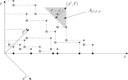
Figure 6. Black dots indicate the position of particles at time zero for the Hammersley process, and dashed lines are their space-time trajectories. Poisson clock rings are marked with squares. Squares (resp. crosses) correspond to creations (resp. annihilations) of kink-antikink pairs for the PNG.The height at the point $(x^{\prime},t^{\prime})$ is determined by the height on the diagonal side of $A_{x^{\prime},t^{\prime},s^{\prime}}$ and by the Poisson points inside the triangle.

Rotating the picture by $45$ degrees, one obtains the graphical representation of the so-called Polynuclear Growth Model [7]. In fact, it is well know that the Hammersley process and the PNG are in bijection. Note however that the initial condition at $t=0$ for the Hammersley process translates into a condition on the line $t^{\prime}=x^{\prime}$ for the PNG (the coordinates $x^{\prime},t^{\prime}$ are as in Figure 6). For the PNG, a deterministic locality property holds, because “kinks” and “anti-kinks” travel at deterministic speed $1$. In other words, the PNG height function at $(x^{\prime},t^{\prime})$ is entirely determined by the Poisson points in the triangular region $A_{x^{\prime},t^{\prime},s^{\prime}}$ of Fig. 6 (with $s^{\prime}<t^{\prime}$) together with the height at time $s^{\prime}$ on a segment $[x^{\prime}-(t^{\prime}-s^{\prime}),x^{\prime}+(t^{\prime}-s^{\prime})]$ (i.e. on the diagonal side of the triangle). By the bijection, we obtain the same property for the Hammersley process and the diagonal side of $A_{x^{\prime},t^{\prime},s^{\prime}}$ is the analog of the set $E_{x,t,\ell}$ of Proposition 3.5. The reason why Proposition 3.5 holds is that, also for the Borodin-Ferrari dynamics, one can establish a bijection with a discretized version of the Gates-Westcott growth model, for which information travels ballistically. The bijection with the Borodin Ferrari dynamics is not discussed explicitly in the literature and we do not describe it here either, as we need only its consequence, Proposition 3.5, of which we give a self-contained proof.

Proof of Proposition 3.5.

We proceed by induction and we assume without loss of generality that $x=0$. Let us start with the case $\ell=1$ (see Figure 7).

For the sake of simplicity, let us write $H(\cdot,t)$ for $H(\cdot,t;h,W)$ and $H^{\prime}(\cdot,t)$ for $H(\cdot,t;h^{\prime},W)$. We want to show:

$$H(\cdot,\cdot)\leq H^{\prime}(\cdot,\cdot)\text{ on }E_{0,t,1}\Rightarrow H(0,\cdot)\leq H^{\prime}(0,\cdot)\text{ on }[t-1,t]\>.$$ (3.9)

Figure 7. Case $\ell=1$ of Proposition 3.5. If $H\leq H^{\prime}$ on the bold lines and points (corresponding to $E_{0,t,1}$), then $H\leq H^{\prime}$ also on the dash line (corresponding to $\{0\}\times(t-1,t]$).

Since height functions are almost surely right-continuous with $-1$ jumps (when a particle jumps), it is enough to show that if at time $t_{0}\in[t-1,t]$, $H(0,t_{0}^{-})=H^{\prime}(0,t_{0}^{-})$ and $H^{\prime}$ decreases by $1$ at $0$, then it is also the case for $H$. By definition of the height function, it means that the left-most particle to the right of $0$ on line $0$ has crossed $0$ at time $t_{0}$ for $H^{\prime}$. We have to show that the same happens for $H$. Two cases can occur:

1. The particle landed at the rightmost position on the left of $x=0$, i.e. at horizontal position $z=-1$ (corresponding to position $(-1/2,-1/2)$ in the coordinates chosen on $G^{*}$). By definition of the height function and of the dynamics, it is easily checked that the left-most particle to the right of $0$ can jump at position $z=-1$ (at time $t_{0}$, for the configuration with height function $H^{\prime}$) if and only if

   $$\left\{\begin{aligned} H^{\prime}((0,-1),t_{0}^{-})-H^{\prime}((-1,-1),t_{0}^{-})&=0\\ H^{\prime}((-1,0),t_{0}^{-})-H^{\prime}((-1,-1),t_{0}^{-})&=0\\ H^{\prime}(0,t_{0}^{-})-H^{\prime}((-1,-1),t_{0}^{-})&=1.\end{aligned}\right.$$

   Since $H(0,t_{0}^{-})=H^{\prime}(0,t_{0}^{-})$ and by assumption $H((-1,-1),t_{0}^{-})\leq H^{\prime}((-1,-1),t_{0}^{-})$, we deduce that

   $$H(0,t_{0}^{-})-H((-1,-1),t_{0}^{-})=1$$

   (recall that from (2.4)-(2.5) that discrete height gradients take values in $\{0,1\}$) and also $H((-1,-1),t_{0}^{-})=H^{\prime}((-1,-1),t_{0}^{-})$. Moreover, since $H((-1,0),t_{0}^{-})\leq H^{\prime}((-1,0),t_{0}^{-})$ and $H((0,-1),t_{0}^{-})\leq H^{\prime}((0,-1),t_{0}^{-})$, we have that

   $$H((-1,0),t_{0}^{-})-H((-1,-1),t_{0}^{-})=H((0,-1),t_{0}^{-})-H((-1,-1),t_{0}^{-})=0$$

   and thus the left-most particle to the right of $0$ for $H$ is also free to jump to position $z=-1$ at time $t_{0}$ and thus $H$ also decreases by $1$ at $0$.

2. The particle landed further to the left than $z=-1$. In this case, the height function $H^{\prime}$ decreases by $1$ at time $t_{0}$ at $0$ but also at $(-1,-1)$. Besides, this implies that there was no particle at position $z=-1$ at time $t_{0}^{-}$. Therefore, we have

   $$H(0,t_{0}) \leq H((-1,-1),t_{0})+1$$

   $$\leq H^{\prime}((-1,-1),t_{0})+1 H\leq H^{\prime} E_{0,t,1}$$ since on

   $$=H^{\prime}((-1,-1),t_{0}^{-}) H^{\prime} 1 (-1,-1) t_{0}$$ decreases by at at time

   $$=H^{\prime}(0,t_{0}^{-})-1 z=-1$$ there was no particle at

   $$=H(0,t_{0}^{-})-1.$$

   Consequently, $H$ also decreased by $1$ at $0$ at time $t_{0}$.

Now let us show the inductive step, as illustrated in Fig. 8: we assume that the result holds for some integer $\ell\geq 1$ and we show that it holds also for $\ell+1$. Let us assume that $H(.,.)\leq H^{\prime}(.,.)\text{ on }E_{0,t,\ell+1}$. All we have to show is that this inequality is also true on $E_{0,t,\ell}$ and conclude by the induction hypothesis.

To show this, we can apply the result (3.9) for $\ell=1$ to all $(y,t-\ell-\frac{y_{1}+y_{2}}{2})$ with $y\in T_{\ell}$ such that $y_{1}+y_{2}$ is even and deduce that $H(y,\cdot)\leq H^{\prime}(y,\cdot)$ on $[t-\ell-\frac{y_{1}+y_{2}}{2}-1,t-\ell-\frac{y_{1}+y_{2}}{2}]$. Next, we apply once more (3.9) to all $(y,t-\ell-\lfloor\frac{y_{1}+y_{2}}{2}\rfloor)$ with $y\in T_{\ell}$ such that $y_{1}+y_{2}$ is odd and deduce that $H(y,\cdot)\leq H^{\prime}(y,\cdot)$ on $[t-\ell-\lfloor\frac{y_{1}+y_{2}}{2}\rfloor-1,t-\ell-\lfloor\frac{y_{1}+y_{2}}{2}\rfloor]$. We get that $H\leq H^{\prime}$ on $E_{0,t,\ell}$ which concludes the proof.

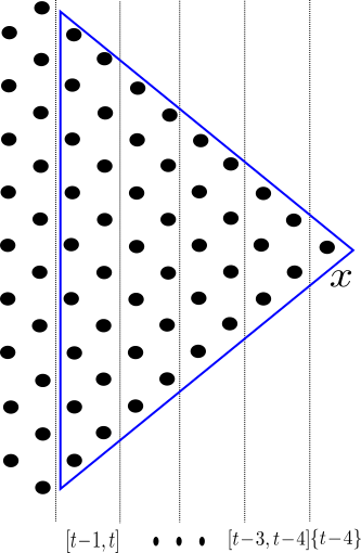
Figure 8. The induction step from $\ell$ to $\ell+1$. At the bottom, we write the time interval on which $H\leq H^{\prime}$ for the positions between the two corresponding vertical lines. The inequalities in the intervals of the left figure are equivalent to $H\leq H^{\prime}$ on $E_{0,t,\ell+1}$ (here with $\ell+1=5$). We begin with applying the case $\ell=1$ in each unit square in the left figure and we deduce the new time intervals on which $H\leq H^{\prime}$ (shown in the figure in the middle). Next, we apply the statement with $\ell=1$ in each unit square of the middle figure and, as suggested on the right figure, we conclude that $H\leq H^{\prime}$ on $E_{0,t,\ell}$.

∎

4. Compactness

4.1. Reducing to a simpler initial condition

From [9, Lemma 2.5] we have that, given $f\in\bar{\Gamma}_{M}$ for some integer $M$ as in the statement of Theorem 2.1 and any $L\in\mathbb{N}$, there exists a natural discrete height function $h_{L}^{f}(x)$ that satisfies (a stronger version of) (2.14): it suffices to set $h_{L}^{f}(x):=\lfloor Lf(x/L)\rfloor$. Then, $h_{L}^{f}\in\Gamma_{M}$ and moreover one has

$$\left|\frac{1}{L}h_{L}^{f}(\lfloor xL\rfloor)-f(x)\right|\leq\frac{1}{L}\qquad\forall x\in\mathbb{R}^{2},$$ (4.1)

which is stronger than (2.14).

A simple consequence of Corollary 3.4 is that it is sufficient to prove Theorem 2.1 for the initial condition $h_{L}^{f}$. Indeed, if $(h_{L})_{L\in\mathbb{N}}\in\Gamma_{M}^{\mathbb{N}}$ converges to $f$ in the sense of (2.14), then by an immediate consequence of Corollary 3.4, for all $T,R\geq 0$,

$$\limsup_{L\to\infty}\sup_{x\in B(0,R),\,t\in[0,T]}\left|\frac{1}{L}H(\lfloor Lx\rfloor,Lt,h_{L},W)-\frac{1}{L}H(\lfloor Lx\rfloor,Lt,h_{L}^{f},W)\right|$$

$$\leq\limsup_{L\to\infty}\sup_{x\in B(0,R+\alpha T)}\left|\frac{1}{L}h_{L}(\lfloor Lx\rfloor)-\frac{1}{L}h_{L}^{f}(\lfloor Lx\rfloor)\right|$$

$$\leq\limsup_{L\to\infty}\sup_{B(0,R+\alpha T)}\left|\frac{1}{L}h_{L}(\lfloor Lx\rfloor)-f(x)\right|+\sup_{B(0,R+\alpha T)}\left|\frac{1}{L}h_{L}^{f}(\lfloor xL\rfloor)-f(x)\right|=0,$$

because of (2.14) and (4.1). Therefore, from now on we will assume that $h_{L}=h_{L}^{f}$.

Definition 4.

For every $f\in\bar{\Gamma}$, every realisation of the Poisson process $W$ and any scaling parameter $L\in\mathbb{N}$, we define the rescaled height function

$$H_{L}(x,t;f,W):=\frac{1}{L}H(\lfloor Lx\rfloor,Lt;h_{L}^{f},W).$$ (4.2)

4.2. Bound on temporal height differences

The goal of this section is to obtain a control on the temporal height differences that will be useful for showing compactness of the sequence $(H_{L}(\cdot,\cdot;f,W))_{L\in\mathbb{N}}$.

Proposition 4.1.

For almost every $W$, for every integer $M$, there exists a constant $C=C(M)$ such that for all $x\in\mathbb{R}^{2}$, $t\geq 0$, $\delta>0$ and all $f\in\bar{\Gamma}_{M}$,

$$\limsup_{L\to\infty}\sup_{s\in[t-\delta,t+\delta]}\left|H_{L}(x,t;f,W)-H_{L}(x,s;f,W)\right|\leq C\sqrt{t+\delta}\,\sqrt{\delta}.$$ (4.3)

Proof.

Let $x\in\mathbb{R}^{2}$, $t\geq 0$, $\delta>0$, $f\in\bar{\Gamma}_{M}$. Since the height functions are non-increasing with time, it is enough to get an upper bound on

$$H_{L}(x,t-\delta;f,W)-H_{L}(x,t+\delta;f,W).$$

The next Lemma relates the height differences to increasing subsequences of Poisson points.

Lemma 4.2.

Let $x\in\mathbb{Z}^{2}$, $s,\tau\geq 0$, $k\in\mathbb{N}$. If $H(x,s;h,W)-H(x,s+\tau;h,W)\geq k$ for some $h\in\Gamma$ and $W$, then there exist increasing subsequences $z_{0}<\cdots<z_{k-1}\leq\bar{z}(x)$, and $s\leq t_{0}<\cdots<t_{k-1}\leq s+\tau$ such that $(z_{i},\bar{\ell}(x),t_{i})\in W$ for all $i$.

For all $n\geq k$, the probability that there exists an increasing sequence in $W$ as above with $z_{0}>\bar{z}(x)-n$ is upper bounded by $\frac{(\tau n)^{k}}{(k!)^{2}}\leq\left(\frac{e^{2}\tau n}{k^{2}}\right)^{k}$.

The proof is easy and is postponed to the end of the section.

With Lemma 4.2, Borel-Cantelli Lemma, and a rational approximation argument it is possible to show that for almost every $W$, for all $M,x,t,\delta$ as in Proposition 4.1, for all $L$ large enough, for all $h\in\Gamma_{M}$,

$$H(\lfloor Lx\rfloor,L(t-\delta);h,\tilde{W})-H(\lfloor Lx\rfloor,L(t+\delta);h,\tilde{W})\leq 2e\sqrt{L2\delta\times L\alpha(t+\delta)},$$ (4.4)

with $\tilde{W}$ the restriction of $W$ to $B(\lfloor Lx\rfloor,L\alpha(t+\delta))\times[0,(t+\delta)L]$ (cf. (3.3)). The rest of the proof follows from Proposition 3.3 and by setting $C(M)=2e\sqrt{2\alpha(M)}$.

∎

Proof of Lemma 4.2.

By definition, if $H(x,s;h,W)-H(x,t;h,W)\geq k$, then $k$ particles crossed $x$ between time $s$ and $t$. We denote by $(p,\ell)$ the label of the left-most particle to the right of $x$ at time $s$ (i.e $\ell=\bar{\ell}(x)$ and $p=\min\{p,\,z_{(p,\ell)}(s)>\bar{z}(x)\}$). Since $k$ particles crossed $x$ in the time interval $[s,t]$, there exist some time $t_{k-1}\in[s,t]$ where particle $(p+k-1,l)$ crossed $x$ and landed at some position $z_{k-1}<\bar{z}(x)$. Necessarily, $(z_{k-1},\ell,t_{k-1})\in W$ (since it corresponds to a jump) and particle $(p+k-2,\ell)$ was strictly on the left of $z_{k-1}$ at time $t_{k-1}$ (otherwise, the jump could not have occurred). This proves the case $k=1$. If $k\geq 2$, since particle $(p+k-2,\ell)$ was on the right of $\bar{z}(x)$ (and $z_{k-1}$) at time $s$, there exists some $t_{k-2}\in[s,t_{k-1}]$ when it jumped strictly on the left of $z_{k-1}$ and landed at some $z_{k-2}<z_{k-1}$ with $(z_{k-2},\ell,t_{k-2})\in W$. The proof proceeds by induction.

The upper bound on the probability that such a sequence exists is standard (see e.g [15, Lemma 4.1]), so we omit it. ∎

4.3. Compactness for almost every realisation of the Poisson process $W$

The goal is to show the following:

Proposition 4.3.

For almost every realisation of $W$ the following holds: every subsequence $(L_{k})_{k\in\mathbb{N}}$ contains a sub-subsequence $(L_{k_{m}})_{m\in\mathbb{N}}$ such that for all function $f\in\bar{\Gamma}$ one has

$$\forall T,R>0\qquad\sup_{\|x\|\leq R,t\in[0,T]}\left|H_{L_{k_{m}}}(x,t;f,W)-H_{\infty}(x,t;f,W)\right|\underset{m\to\infty}{\longrightarrow}0,$$ (4.5)

for some continuous function $H_{\infty}(\cdot,\cdot;f,W)\in\mathcal{C}(\mathbb{R}^{2}\times\mathbb{R}_{+})$.

Proof.

Let us fix $W$ in the event of probability one on which Proposition 4.1 and Corollary 3.4 hold simultaneously. Since ${\bar{\Gamma}}$ is the countable union of the $\bar{\Gamma}_{M}$ and since $\mathbb{R}^{2}\times\mathbb{R}_{+}$ can be written as a countable union of $[-R,R]^{2}\times[0,T]$, modulo a standard diagonal extraction procedure, we can restrict ourselves to the case of $\bar{\Gamma}_{M}$ for a fixed $M$ and of a fixed compact set $[-R,R]^{2}\times[0,T]$.

Let us start by showing the following Lemma where the function $f$ is fixed.

Lemma 4.4.

Let $R,T>0$ and $f\in\bar{\Gamma}_{M}$. For almost every realisation of $W$, the following holds: every subsequence $(L_{k})_{k\in\mathbb{N}}$ contains a sub-subsequence $(L_{k_{m}})_{m\in\mathbb{N}}$ such that

$$\sup_{\|x\|\leq R,t\in[0,T]}\left|H_{L_{k_{m}}}(x,t;f,W)-H_{\infty}(x,t;f,W)\right|\underset{m\to\infty}{\longrightarrow}0,$$ (4.6)

for certain a function $H_{\infty}(\cdot,\cdot;f,W)\in\mathcal{C}([-R,R]^{2}\times[0,T])$.

Proof.

Keeping in mind the ideas of the Arzelà-Ascoli Theorem, we will first show pointwise boundedness and asymptotic equi-continuity with respect to $(x,t)$.

1. Pointwise boundedness: By Proposition 4.1 (with $\delta=t$), the height function grows at most linearly i.e there exists $C^{\prime}>0$ such that

   $$\forall x,t\in\mathbb{R}^{2}\times\mathbb{R}_{+},\qquad\limsup_{L\to\infty}|H_{L}(x,t;f,W)-\underbrace{H_{L}(x,0;f,W)}_{\to f(x)}|\leq C^{\prime}\,t.$$ (4.7)

2. Asymptotic equi-continuity with respect to $x,t$: Equi-continuity in $x$ is automatic because the spatial discrete gradients of the interface are bounded by 1. Thus,

   $$\forall x,y,s\in\mathbb{R}^{2}\times\mathbb{R}^{2}\times\mathbb{R}_{+}\quad\left|H_{L}(x,s;f,W)-H_{L}(y,s;f,W)\right|\leq\|x-y\|+\frac{1}{L}.$$

   Moreover, asymptotic equi-continuity with respect to $t$ is a direct consequence of Proposition 4.1 and thus for all $x,t$, and $\delta>0$,

   $$\limsup_{L\to\infty}\sup_{\begin{subarray}{c}y,\|y-x\|\leq\delta\\ s\in[t-\delta,t+\delta]\end{subarray}}\left|H_{L}(y,s;f,W)-H_{L}(x,t;f,W)\right|\leq\delta+C\sqrt{t+\delta}\sqrt{\delta}.$$ (4.8)

Now, let $(L_{k})_{k\in\mathbb{N}}$ be a subsequence. By pointwise boundedness and by diagonal extraction, we can find a sub-subsequence $(L_{k_{m}})_{m\in\mathbb{N}}$ such that for all $x,t\in\mathcal{S}$, with $\mathcal{S}$ a countable dense countable subset of $[-R,R]^{2}\times[0,T]$, the sequence of real numbers $(H_{L_{k_{m}}}(x,t;f,W))_{m\in\mathbb{N}}$ converges to some limit to some $H_{\infty}(x,t;f,W)$.

Let us extend this limit to the whole $[-R,R]^{2}\times[0,T]$. By asymptotic equi-continuity (4.8) and by density of $\mathcal{S}$, it is not hard to show that for any $(x,t)\in[-R,R]^{2}\times[0,T]$, the sequence of real numbers $(H_{L_{k_{m}}}(x,t;f,W))_{m\in\mathbb{N}}$ is a Cauchy sequence and thus also converges. Consequently, $(H_{L_{k_{m}}}(\cdot,\cdot;f,W))_{m\in\mathbb{N}}$ converges pointwise on $[-R,R]^{2}\times[0,T]$ to some $H_{\infty}(\cdot,\cdot;f,W)$ which is automatically continuous by taking the limit in (4.8).

It remains to show that the convergence is uniform. This is easily done by using compactness of $[-R,R]^{2}\times[0,T]$ and asymptotic equi-continuity (4.8) so we omit the proof.

∎

Let us finish the proof of Proposition 4.3. Since $\bar{\Gamma}_{M}$ is separable for the topology of convergence on all compact sets, we can find a countable dense subset that we call $\mathcal{S}^{\prime}$. By Lemma 4.4 and diagonal extraction, from any subsequence $(L_{k})_{k\in\mathbb{N}}$, we can extract a sub-subsequence $(L_{k_{m}})_{m\in\mathbb{N}}$ such that for any function $g\in\mathcal{S}^{\prime}$, $(H_{L_{k_{m}}}(\cdot,\cdot;g,W))_{m\in\mathbb{N}}$ converges uniformly on $[-R,R]^{2}\times[0,T]$ to a continuous function $H_{\infty}(\cdot,\cdot;g,W)\in\mathcal{C}([-R,R]^{2}\times[0,T])$.

We are going to extend this limit to any $f\in\bar{\Gamma}_{M}$ by showing that $(H_{L_{k_{m}}}(\cdot,\cdot;f,W))_{m\in\mathbb{N}}$ is a Cauchy sequence in the space of functions from $[-R,R]^{2}\times[0,T]$ into $\mathbb{R}$ endowed with the uniform convergence which makes it complete. For this, we will need to use some equi-continuity with respect to $f$. It follows from Corollary 3.4 and from (4.1) that for all $r\geq 0$ and all $f,g\in\bar{\Gamma}_{M}$,

$$\limsup_{L\to\infty}\sup_{\begin{subarray}{c}x\in B(0,r)\\ t\in[0,T]\end{subarray}}\left|H_{L}(x,t;f,W)-H_{L}(x,t;g,W)\right|\leq\sup_{x\in B(0,r+\alpha T)}|f(x)-g(x)|.$$ (4.9)

Fix $r$ large enough such that $B(0,r)$ contains $[-R,R]^{2}$ and fix $f\in\bar{\Gamma}_{M}$. Since the r.h.s of (4.9) can be taken arbitrarily small by choosing $g\in\mathcal{S}^{\prime}$ close enough to $f$ and since $(H_{L_{k_{m}}}(\cdot,\cdot;g,W))_{m\in\mathbb{N}}$ is a Cauchy sequence for the uniform convergence on $[-R,R]^{2}\times[0,T]$, this is also the case for $(H_{L_{k_{m}}}(\cdot,\cdot;f,W))_{m\in\mathbb{N}}$. In conclusion, for any $f\in\bar{\Gamma}_{M}$, $(H_{L_{k_{m}}}(\cdot,\cdot;f,W))_{m\in\mathbb{N}}$ converges uniformly on $[-R,R]^{2}\times[0,T]$ to a continuous function $H_{\infty}(\cdot,\cdot;f,W)\in\mathcal{C}([-R,R]^{2}\times[0,T])$. This concludes the proof of Proposition 4.3. ∎

5. Identification of the limit

All along this section, we will denote by $H_{\infty}$ any continuous limit obtained by extraction of the sequence of rescaled height functions $(H_{L})_{L\in\mathbb{N}}$ as in Proposition 4.3. In order to finish the proof of Theorem 2.1, we need to show that there is only one possible limit $H_{\infty}(\cdot,\cdot;f,W)$that coincides almost surely with the unique viscosity solution of (2.16).

5.1. Properties of limit points

First of all, let us show some properties of $H_{\infty}$, inherited from those of the the microscopic dynamics.

Proposition 5.1 (Vertical translation invariance).

For almost every $W$, every $f\in\bar{\Gamma}$ and $c\in\mathbb{R}$,

$$H_{\infty}(\cdot,\cdot;f+c,W)=H_{\infty}(\cdot,\cdot;f,W)+c.$$

Proof.

From the definition of $h_{L}^{f}=\lfloor Lf(x/L)\rfloor$, we observe that $h_{L}^{f}+\lfloor Lc\rfloor\leq h_{L}^{f+c}\leq h_{L}^{f}+\lfloor Lc\rfloor+1$. By Proposition 3.1, we deduce that

$$H_{L}(\cdot,\cdot;f,W)+\frac{\lfloor Lc\rfloor}{L}\leq H_{L}(\cdot,\cdot;f+c,W)\leq H_{L}(\cdot,\cdot;f,W)+\frac{\lfloor Lc\rfloor+1}{L},$$

which concludes the proof by taking the limit when $L$ goes to infinity. ∎

Proposition 5.2 (Weak locality).

For almost all $W$, all $R,T>0$, all integer $M$ and all $f,g\in\bar{\Gamma}_{M}$,

$$\sup_{{x\in B(0,R)},t\in[0,T]}\left|H_{\infty}(x,t;f,W)-H_{\infty}(x,t;g,W)\right|\leq\sup_{x\in B(0,R+\alpha T)}|f(x)-g(x)|.$$ (5.1)

Proof.

It suffices to take the limit when $L$ goes to infinity of (4.9). ∎

Now, we are going to show a continuous version of Proposition 3.5. We first have to introduce some notations. For all $x\in\mathbb{R}^{2}$ and $t>\delta>0$, we define $\bar{T}_{\delta},\bar{E}_{\delta}$ and $\bar{E}_{x,t,\delta}$ the continuous versions of $T_{\ell}$, $E_{\ell}$ et $E_{x,t,\ell}$ by

$$\bar{T}_{\delta} :=\{y\in\mathbb{R}^{2},\quad y_{1}\leq 0,\>y_{2}\leq 0,\>-2\delta\leq y_{1}+y_{2}\leq 0\}\subseteq\mathbb{R}^{2}$$ (5.2)

$$\bar{E}_{\delta} :=\{(y_{1},y_{2},-\delta-(y_{1}+y_{2})/2),\quad y\in\bar{T}_{\delta}\}\subseteq\mathbb{R}^{2}\times\mathbb{R}$$

$$\bar{E}_{x,t,\delta} :=(x,t)+\bar{E}_{\delta}\subseteq\mathbb{R}^{2}\times\mathbb{R}_{+}.$$

Proposition 5.3 (Space-time locality).

For almost every $W$, every $x\in\mathbb{R}^{2}$, every $t>\delta>0$ and every $f,g\in\bar{\Gamma}$,

$$\left(H_{\infty}(\cdot,\cdot;f,W)\leq H_{\infty}(\cdot,\cdot;g,W)\>\text{on }\bar{E}_{x,t,\delta}\right)\Rightarrow H_{\infty}(x,t;f,W)\leq H_{\infty}(x,t;g,W)$$

Proof.

The proof relies on Proposition 3.5 and a continuity argument. Assume that $H_{\infty}(\cdot,\cdot;f,W)\leq H_{\infty}(\cdot,\cdot;g,W)$ on $\bar{E}_{x,t,\delta}$. Fix $\varepsilon>0$. By continuity of these functions and by compactness of $\bar{E}_{x,t,\delta}$, there exists $\eta>0$ such that

$$H_{\infty}(\cdot,\cdot;f,W)\leq H_{\infty}(\cdot,\cdot;g,W)+\varepsilon\>\text{on $\bar{E}_{x,t,\delta}^{\eta}$},$$

where $\bar{E}_{x,t,\delta}^{\eta}$ is the set of points a distance less than $\eta$ from $\bar{E}_{x,t,\delta}$. By compactness of $\bar{E}_{x,t,\delta}^{\eta}$ and by uniform convergence on all compact sets of the sequences $H_{L}(\cdot,\cdot;f,W)$ and $H_{L}(\cdot,\cdot;g+3\varepsilon,W)$, for all $L$ large enough, the following inequalities hold on $\bar{E}_{x,t,\delta}^{\eta}$:

$$H_{L}(\cdot,\cdot;f,W) \leq H_{\infty}(\cdot,\cdot;f,W)+\varepsilon\leq H_{\infty}(\cdot,\cdot;g,W)+2\varepsilon$$

$$=H_{\infty}(\cdot,\cdot;g+3\varepsilon,W)-\varepsilon\leq H_{L}(\cdot,\cdot;g+3\varepsilon,W),$$

where we used Proposition 5.1 in the equality in the second line. Then, since we enlarged $\bar{E}_{x,t,\delta}$ by $\eta>0$, it is not hard to check that, for all $L$ large enough,

$$E_{\lfloor Lx\rfloor,Lt,\lfloor L\delta\rfloor}\subseteq\{(\lfloor Ly\rfloor,Ls),\,(y,s)\in\bar{E}_{x,t,\delta}^{\eta}\},$$

and thus $H_{L}(\cdot,\cdot;h_{L}^{f},W)\leq H_{L}(\cdot,\cdot;h_{L}^{g+3\varepsilon},W)$ on $E_{\lfloor Lx\rfloor,Lt,\lfloor L\delta\rfloor}$. By Proposition 3.5, for all $\varepsilon>0$, for all $L$ large enough, we have

$$H(\lfloor Lx\rfloor,Lt;h_{L}^{f},W)\leq H(\lfloor Lx\rfloor,Lt;h_{L}^{g+3\varepsilon},W).$$

Dividing by $L$ and taking the limit when $L\to\infty$ yields that for all $\varepsilon>0$,

$$H_{\infty}(x,t;f,W)\leq H_{\infty}(x,t;g+3\varepsilon,W),$$

and the proof follows by letting $\varepsilon$ go to $0$ and using Proposition 5.1 again. ∎

Finally, we need to need the hydrodynamic limit in the easy case where the initial profile is linear.

Proposition 5.4 (Hydrodynamic limit for linear profiles).

For $\rho\in\mathbb{T}$, we let $f_{\rho}(x):=\rho\cdot x$. For almost every $W$,

$$H_{\infty}(\cdot,t;f_{\rho},W)=f_{\rho}-v(\rho)\,t\qquad\forall t\geq 0,\>\forall\rho\in\mathbb{T}.$$ (5.3)

Proof.

Consider first $\rho$ in the interior of $\mathbb{T}$ and let

$$H^{+}_{\infty}(x,t;f_{\rho},W):=\limsup_{L\to\infty}H_{L}(x,t;f_{\rho},W)$$

and analogously with the liminf for $H^{-}_{\infty}(x,t;f_{\rho},W)$. We will prove that, for any given $x,t$, one has $W$-a.s.

$$H^{+}_{\infty}(x,t;f_{\rho},W)\leq f_{\rho}(x)-v(\rho)t,$$ (5.4)

(an analogous statement holds for $H^{-}_{\infty}(x,t;f_{\rho},W)$). Given this, it is then easy to deduce that (5.3) holds, $W$-a.s., simultaneously for all $x$ and for all $t$, using the continuity of $(x,t)\mapsto H_{\infty}(x,t;f_{\rho},W)$. Moreover, by continuity of $\rho\mapsto v(\rho)$ and $\rho\mapsto H_{\infty}(x,t;f_{\rho},W)$ on $\mathbb{T}$ (thanks to Proposition 5.2), we can also deduce that (5.3) holds simultaneously for all $\rho\in\mathbb{T}$.

Let us fix $\rho\in\overset{\circ}{\mathbb{T}}$ and $x,t$ (we assume without loss of generality that $x=0$) and let us prove that (5.4) holds $W$-as. First of all, we replace the initial condition $h_{L}^{f_{\rho}}$ by a (random) initial condition, that we call $h^{stat}$ (“stat” for “stationary”), sampled from the stationary measure $\pi_{\rho}$ with average slope $\rho$, with height fixed to $\delta L/2$ at position $x=0$. We recall from [17] that $\pi_{\rho}$ corresponds to the translation invariant Gibbs measure on rhombus tilings of the plane with average slope $\rho$ [8] and that it is a time-stationary measure for the interface gradients. Note that the $L$-dependence of $h^{stat}$ is trivial: only the height offset is $L$-dependent. We call $H^{stat}_{L}(\cdot,t;\rho,W)$ the corresponding (space-time rescaled) height function at (macroscopic) time $t$, in analogy with (4.2). It is well known that, for any $R>0$, one has $\pi_{\rho}$-a.s. that

$$h^{stat}\geq h^{f_{\rho}}_{L}=\lfloor\rho\cdot x\rfloor\;\text{ on }\;B(0,LR),\;\text{for $L$ large enough}.$$ (5.5)

Given a positive constant $C$, let us consider the localised dynamics where the Poisson clocks outside the ball $B(0,LC)$ are turned off in the time interval $[0,Lt]$, i.e., where $W$ is replaced by $\tilde{W}:=W\cap\left(B(0,LC)\times[0,Lt]\right)$. By local monotonicity (more precisely, apply [9, Th. 5.10]) and by (5.5), we deduce that

$$H^{stat}_{L}(0,t;\rho,\tilde{W})\geq H_{L}(0,t;f_{\rho},\tilde{W}),\;\text{for $L$ large enough}.$$

Now, from Proposition 3.3 we have that $W$-a.s.,

$$H_{L}(0,t;f_{\rho},\tilde{W})=H_{L}(0,t;f_{\rho},W),\;\text{for $L$ large enough},$$

if $C$ is chosen large enough. Similarly, one has almost surely with respect to the joint law of $W$ and of the initial condition $h^{stat}$,

$$H^{stat}_{L}(0,t;\rho,\tilde{W})=H^{stat}_{L}(0,t;\rho,W),\;\text{for $L$ large enough}.$$

This follows (again, for $C$ large enough) from [9, Prop. 5.13]. In conclusion, we get that almost surely with respect to the joint law of $W$ and of $h^{stat}$,

$$H^{stat}_{L}(0,t;\rho,W)\geq H_{L}(0,t;f_{\rho},W),\;\text{for $L$ large enough}$$ (5.6)

and therefore it is enough to show (5.4) for $H^{stat}$ instead of $H$.

By Borel-Cantelli Lemma, it is enough to prove the summability in $L$ of

$$\mathbb{P}(H^{stat}_{L}(0,t;\rho,W)\geq-v(\rho)t+\delta)$$ (5.7)

$$=\mathbb{P}(H^{stat}_{L}(0,t;\rho,W)-H^{stat}_{L}(0,0;\rho,W)\geq-v(\rho)t+\delta/2),$$

for any $\delta>0$ where now $\mathbb{P}$ is the joint law of the process and of the initial condition. On the one hand, it follows from [17, 4] that $-v(\rho)t$ is nothing but the average growth:

$$\mathbb{E}\left[H^{stat}_{L}(0,t;\rho,W)-H^{stat}_{L}(0,0;\rho,W)\right]=-v(\rho)t.$$ (5.8)

On the other hand, [5, Th. 2.2] showed that $\mathrm{Var}\left(H^{stat}(0,t,\rho)-H^{stat}(0,0,\rho)\right)=\mathrm{O}(\log t)$ which implies that

$$\mathrm{Var}\left(H^{stat}_{L}(0,t;\rho,W)-H^{stat}_{L}(0,0;\rho,W)\right)=\underset{L\to\infty}{\mathrm{O}}\left(L^{-2}\log L\right)$$ (5.9)

which is summable in $L$. The rest of the proof follows from Chebyshev’s inequality. ∎

5.2. Viscosity solution

Let us show the following:

Proposition 5.5.

For almost every $W$, the following holds: for every $f\in\bar{\Gamma}$, every $(x,t)\in\mathbb{R}^{2}\times\mathbb{R}_{>0}$ and every smooth function $\varphi$ of space and time such that $H_{\infty}(x,t;f,W)=\varphi(x,t)$ and $H_{\infty}(\cdot,\cdot;f,W)\leq\varphi$ (resp. $\geq\varphi$) in a neighborhood of $(x,t)$,

$$\text{if }\nabla\varphi(x,t)\in\mathbb{T},\text{ then }\partial_{t}\varphi(x,t)+v(\nabla\varphi(x,t))\leq 0\quad(\text{resp.}\geq 0).$$ (5.10)

Remark 4.

Observe that, because of the restriction $\nabla\varphi(x,t)\in\mathbb{T}$, the statement is a priori weaker than saying that $H_{\infty}$ is a viscosity solution in the usual sense.

Proof.

Suppose that $H_{\infty}(x,t;f,W)=\varphi(x,t)$, $H_{\infty}(\cdot,\cdot;f,W)\leq\varphi$ in a neighbourhood of $(x,t)$ (the case $H_{\infty}(\cdot,\cdot;f,W)\geq\varphi$ is similar, so we will not treat it) and $\nabla\varphi(x,t)\in\mathbb{T}$. Let us start by replacing $\varphi$ by an affine function $\psi$ by setting for all $y\in\mathbb{R}^{2}$ et $s\geq-t$

$$\psi(x+y,t+s):=\varphi\left(x,t\right)+y_{1}\,\partial_{x_{1}}\varphi(x,t)+y_{2}\,\partial_{x_{2}}\varphi(x,t)+s\,\partial_{t}\varphi(x,t).$$ (5.11)

By Taylor expansion at order $2$, there exists some $C>0$ such that for all small enough $\delta$ and all $\|y\|\leq\delta$, $|s|\leq\delta$,

$$\left|\psi(x+y,t+s)-\varphi(x+y,t+s)\right|\leq C\delta^{2}.$$ (5.12)

From this inequality, we deduce that for all small enough $\delta$,

$$H_{\infty}(\cdot,\cdot;f,W)\leq\psi+C\delta^{2}\quad\text{ on }\bar{E}_{x,t,\delta}.$$ (5.13)

Now, we need the following Lemma in order to apply Proposition 5.3 afterwards.

Lemma 5.6.

There exists $\rho=\rho(x,t)\in\mathbb{T}$ and, for every $\delta>0$ small enough, there exists $c_{\delta}=c_{\delta}(x,t)\in\mathbb{R}$ such that

$$H_{\infty}(\cdot,\cdot;f_{\rho}+c_{\delta},W)=\psi+C\delta^{2}\quad\text{ on }\bar{E}_{x,t,\delta}.$$ (5.14)

The values of $\rho$ and $c_{\delta}$ are uniquely determined by the conditions

$$\left\{\begin{aligned} \rho_{1}-\rho_{2}&=\partial_{x_{1}}\varphi(x,t)-\partial_{x_{2}}\varphi(x,t)\\ \rho_{1}+\rho_{2}+v(\rho)&=\partial_{x_{1}}\varphi(x,t)+\partial_{x_{2}}\varphi(x,t)-\partial_{t}\varphi(x,t)\\ c_{\delta}&=\varphi(x,t)-\delta\,\partial_{t}\varphi(x,t)-f_{\rho}(x)+v(\rho)(t-\delta)+C\delta^{2}.\end{aligned}\right.$$ (5.15)

Let us first admit this Lemma and conclude the proof of Proposition 5.5. By Proposition 5.3, inequality (5.13) and Lemma 5.6,

$$\varphi(x,t) =H_{\infty}(x,t;f,W)\leq H_{\infty}(x,t;f_{\rho}+c_{\delta},W)$$

$$=f_{\rho}(x)+c_{\delta}-v(\rho)t$$ by Proposition 5.4

$$=\varphi(x,t)-\delta\,\partial_{t}\varphi(x,t)-\delta\,v(\rho)+C\delta^{2}$$ by (5.15).

Since this holds for all small enough $\delta>0$, we finally get that

$$\partial_{t}\varphi(x,t)+v(\rho)\leq 0.$$ (5.16)

Now, combining (5.16) and the second equality in (5.15),

$$\partial_{x_{1}}\varphi(x,t)+\partial_{x_{2}}\varphi(x,t)\leq\rho_{1}+\rho_{2}.$$ (5.17)

Then, since $v$ is increasing with respect to $\rho_{1}+\rho_{2}$ (see Remark 1) and since $\rho_{1}-\rho_{2}=\partial_{x_{1}}\varphi(x,t)-\partial_{x_{2}}\varphi(x,t)$, we deduce that

$$v(\nabla\varphi(x,t))\leq v(\rho).$$ (5.18)

Finally, from (5.16), we get what we wanted:

$$\partial_{t}\varphi(x,t)+v(\nabla\varphi(x,t))\leq 0.$$ (5.19)

∎

Proof of Lemma 5.6.

Let us look for a condition on $\rho$ and $c_{\delta}$ such that (5.14) is satisfied. On the one hand,

$$\psi\left(x+y,t-\delta-\frac{y_{1}+y_{2}}{2}\right)=\varphi(x,t)+y_{1}\partial_{x_{1}}\varphi(x,t)+y_{2}\partial_{x_{2}}\varphi(x,t)-\left(\frac{y_{1}+y_{2}}{2}+\delta\right)\partial_{t}\varphi(x,t),$$ (5.20)

and on the other hand, by Propositions 5.4 and 5.1,

$$H_{\infty}\left(x+y,t-\delta-\frac{y_{1}+y_{2}}{2};f_{\rho}+c_{\delta},W\right)=\rho\cdot(x+y)+c_{\delta}-v(\rho)\left(t-\delta-\frac{y_{1}+y_{2}}{2}\right).$$ (5.21)

Therefore, it is necessary and sufficient to find $\rho\in\mathbb{T}$ and $c_{\delta}\in\mathbb{R}$ such that

$$\left\{\begin{aligned} \rho_{1}+\frac{1}{2}v(\rho)&=\partial_{x_{1}}\varphi(x,t)-\frac{1}{2}\partial_{t}\varphi(x,t)\\ \rho_{2}+\frac{1}{2}v(\rho)&=\partial_{x_{2}}\varphi(x,t)-\frac{1}{2}\partial_{t}\varphi(x,t)\\ \rho\cdot x+c_{\delta}-v(\rho)(t-\delta)&=\varphi(x,t)-\delta\,\partial_{t}\varphi(x,t)+C\delta^{2}.\end{aligned}\right.$$ (5.22)

Notice that this system is equivalent to (5.15). We are going to show that this system has a unique solution $(\rho,c_{\rho})$ with $\rho\in\mathbb{T}$ and $c_{\delta}\in\mathbb{R}$. With the change of coordinate $\rho_{h}=\rho_{1}+\rho_{2}$, $\rho_{v}=\rho_{1}-\rho_{2}$ and $\hat{v}(\rho_{h},\rho_{v}):=v((\rho_{h}+\rho_{v})/2,(\rho_{h}-\rho_{v})/2)$, it is equivalent to looking for $(\rho_{h},\rho_{v})$ such that $|\rho_{v}|\leq\rho_{h}<1$ and

$$\left\{\begin{aligned} \rho_{v}&=\partial_{x_{1}}\varphi(x,t)-\partial_{x_{2}}\varphi(x,t)\\ \rho_{h}+\hat{v}(\rho_{h},\rho_{v})&=\partial_{x_{1}}\varphi(x,t)+\partial_{x_{2}}\varphi(x,t)-\partial_{t}\varphi(x,t).\end{aligned}\right.$$ (5.23)

The first equation fixes the value of $\rho_{v}=\partial_{x_{1}}\varphi(x,t)-\partial_{x_{2}}\varphi(x,t)$ which belongs to $]-1,1[$ (since $\nabla\varphi(x,t)\in\mathbb{T}$ by assumption). Now, by Remark 1, for fixed $\rho_{v}$, the function $\rho_{h}\mapsto\rho_{h}+\hat{v}(\rho_{h},\rho_{v})$ is strictly increasing and thus is a bijection from $[|\rho_{v}|,1)$ to $[|\rho_{v}|,+\infty)$. (The reason behind this fact can be traced back to the bijection between the Borodin-Ferrari dynamics and the (discretized) Gates-Westcott one, mentioned in Section 3.2). Besides, since $H_{\infty}(\cdot,\cdot;f,W)\leq\varphi$ on a neighbourhood of $(x,t)$ with equality at $(x,t)$ and since $H_{\infty}(\cdot,\cdot;f,W)$ is non-increasing w.r.t time, we deduce that necessarily $\partial_{t}\varphi(x,t)\leq 0$. Moreover, $\partial_{x_{1}}\varphi(x,t),\partial_{x_{2}}\varphi(x,t)\geq 0$ (since $\nabla\varphi(x,t)\in\mathbb{T}$ by assumption) and thus $\partial_{x_{1}}\varphi(x,t)+\partial_{x_{2}}\varphi(x,t)\geq|\partial_{x_{1}}\varphi(x,t)-\partial_{x_{2}}\varphi(x,t)|$. Consequently, we have

$$\partial_{x_{1}}\varphi(x,t)+\partial_{x_{2}}\varphi(x,t)-\partial_{t}\varphi(x,t)\in[|\rho_{v}|,+\infty[$$

and thus there exists (a unique) $\rho_{h}\in[|\rho_{v}|,1)$ satisfying the second equation in (5.23). This finally imposes the value of $\rho$ and of $c_{\delta}$ (by the third equation in  (5.15)). ∎

5.3. Uniqueness and conclusion

To conclude this section, we need to show that there is at most one viscosity solution in the sense of Proposition 5.5.

Proposition 5.7.

There exists a most one continuous function $u^{\prime}$ on $\mathbb{R}^{2}\times\mathbb{R}_{+}$ with initial condition $f\in\bar{\Gamma}$ which is a viscosity solution of (2.16) in the sense of (5.10), which satisfies the following gradient bounds:

$$0\leq\frac{u^{\prime}(x+\lambda\,e,t)-u^{\prime}(x,t)}{\lambda}\leq 1\text{ for any }e\in\{(1,0),(0,1),(1,1)\},x\in\mathbb{R}^{2},\lambda\geq 0,$$ (5.24)

and which grows at most linearly in time, i.e there exists a finite $S>0$ such that

$$0\leq f(x)-u^{\prime}(x,t)\leq St\text{ for every }x\in\mathbb{R}^{2},t\geq 0.$$ (5.25)

Moreover, $u^{\prime}$ coincides with $u$, the unique viscosity solution of (2.16).

The proof of this Proposition is postponed to the Appendix. Since any limit $H_{\infty}(\cdot,\cdot;f,W)$ satisfies (5.24) (by taking the limit in the gradient bounds (2.4) (2.5) and (2.6) satisfied by discrete height functions) and (5.25) (by taking the limit in (4.7) and by monotonicity w.r.t time), we deduce the following Corollary.

Corollary 5.8.

For almost every $W$ and for any limit $H_{\infty}$ as in Proposition 4.3 we have that for every $f\in\bar{\Gamma}$, $(x,t)\mapsto H_{\infty}(x,t;f,W)$ is the unique viscosity solution of (2.16).

To complete the proof of Theorem 2.1 it is sufficient to put together what we have obtained so far.

Proof of Theorem 2.1.

Let us fix $W$ in an event of probability one such that Proposition 4.3 and Corollaries 3.4 and 5.8 hold simultaneously. Let $f\in\bar{\Gamma}_{M}$. By the discussion in Section 4.1, without loss of generality, we can replace the sequence of initial height profiles $h_{L}$ approaching $f$ as in Theorem 2.1 by $h_{L}^{f}$. Assume that for some $T,R>0$, the limit (2.15) does not hold, i.e, there exists $\varepsilon>0$ and a subsequence $(L_{k})_{k\in\mathbb{N}}$ such that

$$\forall k\in\mathbb{N},\>\sup_{\|x\|\leq R,t\in[0,T]}\left|H_{L_{k}}(x,t;f,W)-u(x,t)\right|\geq\varepsilon,$$ (5.26)

where $u$ is the unique viscosity solution of (2.16). Then, by Proposition 4.3, we can extract a sub-subsequence $(L_{k_{m}})_{m\in\mathbb{N}}$ such that for all $g\in\bar{\Gamma}$, the sequence of rescaled height functions $(H_{L_{k_{m}}}(\cdot,\cdot;g,W))_{m\in\mathbb{N}}$ converges uniformly on all compact sets to some continuous function $H_{\infty}(\cdot,\cdot;g,W)$. By Corollary 5.8, $(x,t)\mapsto H_{\infty}(x,t;f,W)$ has to be equal to $u$. This is in contradiction with (5.26). ∎

Appendix A Proof of Proposition 5.7

The proof relies on an adaptation of a standard doubling of variables argument (see e.g [2, p.64-72]).

Let $u^{\prime}$ be a continuous function initially equal to $f\in\bar{\Gamma}_{M}$ for some integer $M$ and which is a solution in the sense of Eq. (5.10) satisfying (5.24) and (5.25). Let $u$ be the unique viscosity solution of (2.16). As explained in Remark 3, $u(\cdot,t)$ stays in $\bar{\Gamma}_{M}$ for all $t$ so in particular, it satisfies (5.24) and by the comparison principle (and since $v$ is positive on $\mathbb{T}_{M}$), it satisfies (5.25) with $S_{M}:=\max_{\rho\in\mathbb{T}_{M}}v(\rho)$.

Let us start by showing that $u\leq u^{\prime}$. Suppose the contrary i.e $u(x,t)>u^{\prime}(x,t)$ for some $x,t$. Therefore, we can fix $T\geq t$ and arbitrary small $\eta,\beta>0$ such that the supremum

$$M:=\sup_{x,t\in\mathbb{R}^{2}\times[0,T]}(u(x,t)-u^{\prime}(x,t)-\eta\,t-2\beta\,\|x\|^{2})$$ (A.1)

is positive. Now, we introduce the function

$$\psi(x,t,y,s):=(x,t,y,s)\mapsto u(x,t)-u^{\prime}(y,s)-\frac{\|x-y\|^{2}}{\varepsilon^{2}}-\frac{|t-s|^{2}}{\alpha^{2}}-\eta\,t-\beta\,(\|x\|^{2}+\|y\|^{2}),$$

where $\varepsilon,\alpha$ are penalisation parameters that make the supremum of $\psi$ looks like $M$ for small $\varepsilon,\alpha$.

Lemma A.1.

Let us fix positive $T,\eta,\beta$ such that $M>0$. For any $\varepsilon,\alpha\in[0,1]$, $\psi$ attains its maximum $\bar{M}$ on a point $(\bar{x},\bar{t},\bar{y},\bar{s})\in\mathbb{R}^{2}\times[0,T]\times\mathbb{R}^{2}\times[0,T]$. Moreover,

1. $0<M\leq\bar{M}$

2. $\|\bar{x}-\bar{y}\|^{2}\leq C\varepsilon^{2}$, $|\bar{t}-\bar{s}|^{2}\leq C\alpha^{2}$ and $\|\bar{x}\|^{2}+\|\bar{y}\|^{2}\leq C\,\beta^{-1}$ with $C=2(ST+1)$

3. $\bar{M}\underset{\varepsilon,\alpha\to 0}{\longrightarrow}M$

4. $\bar{t},\bar{s}>0$ for all $\varepsilon,\alpha$ small enough.

Let us admit this Lemma first and conclude the proof of Proposition 5.7. The function defined on $\mathbb{R}^{2}\times[0,T]$ by

$$(x,t)\mapsto u(x,t)-\varphi^{(1)}(x,t)$$

has a local maximum at $(\bar{x},\bar{t})$ where

$$\varphi^{(1)}(x,t):=u^{\prime}(\bar{y},\bar{s})+\frac{\|x-\bar{y}\|^{2}}{\varepsilon^{2}}+\frac{|t-\bar{s}|^{2}}{\alpha^{2}}+\eta\,t+\beta(\|x\|^{2}+\|\bar{y}\|^{2}).$$

Therefore, since $u$ is solution of viscosity of (2.16), and by point $(4)$ of Lemma A.1, we have for all $\varepsilon,\alpha$ small enough,

$$\partial_{t}\varphi^{(1)}(\bar{x},\bar{t})+v(\nabla\varphi^{(1)}(\bar{x},\bar{t}))\leq 0.$$ (A.2)

Remark 5.

To be precise, we need to ensure that the viscosity inequality satisfied by $u$ is still valid if the local optimum on $\mathbb{R}^{2}\times[0,T]$ is attained at the border $\bar{t}=T$. This is proven for example in [2, Lemma 5.1] and the same proof can be easily adapted to the case of $u^{\prime}$.

Now, the function defined on $\mathbb{R}^{2}\times[0,T]$ by

$$(y,s)\mapsto u^{\prime}(y,s)-\varphi^{(2)}(y,s)$$

has a local minimum at $(\bar{y},\bar{s})$ where

$$\varphi^{(2)}(y,s):=u(\bar{x},\bar{t})-\frac{\|\bar{x}-y\|^{2}}{\varepsilon^{2}}-\frac{|\bar{t}-s|^{2}}{\alpha^{2}}-\eta\,\bar{t}-\beta(\|\bar{x}\|^{2}+\|y\|^{2}).$$

In order to use the viscosity inequality (5.10) satisfied by $u^{\prime}$, we first have to make sure that $\nabla\varphi^{(2)}(\bar{y},\bar{s})\in\mathbb{T}$. From (5.24) and since $u^{\prime}-\varphi^{(2)}$ has a local minimum at $(\bar{y},\bar{s})$, it is easy to see that $\nabla\varphi^{(2)}(\bar{y},\bar{s})$ is necessarily in the closure of $\mathbb{T}$. We still have to make sure that it stays away from the diagonal $\{\rho_{1}+\rho_{2}=1\}$.

The idea is to show that $\nabla\varphi^{(2)}(\bar{y},\bar{s})$ is close to $\nabla\varphi^{(1)}(\bar{x},\bar{t})$ which is in $\mathbb{T}_{M}$ (because $u(\cdot,t)\in\bar{\Gamma}_{M}$ for all $t$ as said in Remark 3 and because $u-\varphi^{(1)}$ has a local maximum at $(\bar{x},\bar{t})$). By computing the gradients, we find that

$$\|\nabla\varphi^{(1)}(\bar{x},\bar{t})-\nabla\varphi^{(2)}(\bar{y},\bar{s})\|=2\beta\left\|\bar{x}-\bar{y}\right\|\leq 4\sqrt{C\beta}$$ (A.3)

where the last inequality is due to point $(2)$ of Lemma A.1. This shows that if $\beta$ is chosen small enough, we have that for all $\varepsilon,\alpha$ small enough,

$$\nabla\varphi^{(2)}(\bar{y},\bar{s})\in\mathbb{T}_{M+1}\subseteq\mathbb{T}.$$ (A.4)

Therefore, by (5.10),

$$\partial_{s}\varphi^{(2)}(\bar{y},\bar{s})+v(\nabla\varphi^{(2)}(\bar{y},\bar{s}))\geq 0.$$ (A.5)

Combining (A.2) and (A.5), we get that for all $\varepsilon,\alpha$ small enough,

$$\eta+v(\nabla\varphi^{(1)}(\bar{x},\bar{t}))-v(\nabla\varphi^{(2)}(\bar{y},\bar{s}))\leq 0.$$ (A.6)

Finally, as noticed in Remark 1, $v$ is Lipschitz on $\mathbb{T}_{M+1}$. Therefore, there exists a constant $K>0$ such that for all $\varepsilon,\alpha$ small enough,

$$\left|v(\nabla\varphi^{(1)}(\bar{x},\bar{t}))-v(\nabla\varphi^{(2)}(\bar{y},\bar{s}))\right|\leq K\,\|\nabla\varphi^{(1)}(\bar{x},\bar{t})-\nabla\varphi^{(2)}(\bar{y},\bar{s})\|\leq K4\sqrt{C\beta},$$

because of (A.3). By (A.6), we get that

$$\eta-4K\sqrt{C\beta}\leq 0$$

which is a contradiction for $\beta$ small, since $\eta$ is strictly positive and $C,K$ are independent of $\eta,\beta$. We conclude that $u\leq u^{\prime}$ on $\mathbb{R}^{2}\times\mathbb{R}_{+}$.

Although $u$ and $u^{\prime}$ don’t play symmetric roles, we omit the proof that $u^{\prime}\leq u$ on $\mathbb{R}^{2}\times\mathbb{R}_{+}$ since it is very similar.

Proof of Lemma A.1.

Let us first show that the maximum of $\psi$ is attained. We have for all $x,y\in\mathbb{R}^{2}$ and all $t,s\in[0,T]$,

$$u(x,t)-u^{\prime}(y,s) \leq|u(x,t)-u(y,t)|+u(y,t)-u^{\prime}(y,s)$$ (A.7)

$$\leq\|x-y\|+u(y,0)+S\,T-u^{\prime}(y,0)=\|x-y\|+S\,T$$

where in the second inequality we used that $u$ satisfies (5.24) hence is $1$-Lipschitz and is non-increasing w.r.t time and that $u^{\prime}$ satisfies (5.25). We also used $u(y,0)=u^{\prime}(y,0)=f(y)$ in the last step. As a consequence,

$$\psi(x,t,y,s)\leq\|x-y\|+ST-\beta\,(\|x\|^{2}+\|y\|^{2})$$

which tends to $-\infty$ when $\|x\|,\|y\|\to+\infty$. By continuity of $\psi$, its maximum is attained at some $(\bar{x},\bar{t},\bar{y},\bar{s})$. Now, for any $x,t$,

$$\psi(\bar{x},\bar{t},\bar{y},\bar{s})\geq\psi(x,t,x,t)=u(x,t)-u^{\prime}(x,t)-\eta t-2\beta\|x\|^{2},$$

which shows the first point of Lemma A.1 by taking the supremum with respect to $x,t$.

Then, from the positivity of $\bar{M}$, we deduce that

$$\frac{\|\bar{x}-\bar{y}\|^{2}}{2\varepsilon^{2}}+\frac{|\bar{t}-\bar{s}|^{2}}{\alpha^{2}}+\beta\,(\|\bar{x}\|^{2}+\|\bar{y}\|^{2}) \leq u(\bar{x},\bar{t})-u^{\prime}(\bar{y},\bar{s})-\frac{\|\bar{x}-\bar{y}\|^{2}}{2\varepsilon^{2}}$$

$$\stackrel{{\scriptstyle\text{by \eqref{eq:boundu-u'}}}}{{\leq}}\|\bar{x}-\bar{y}\|+ST-\frac{\|\bar{x}-\bar{y}\|^{2}}{2\varepsilon^{2}}\leq ST+1=:\frac{C}{2}$$

where the last inequality hold for all $\varepsilon\leq 1$. This shows point $(2)$.

From point $(2)$, we know that for fixed $\beta$ and for any $\varepsilon,\alpha\in[0,1]$, $(\bar{x},\bar{t}),(\bar{y},\bar{s})$ stay in a compact set so, modulo sub-sequences, we can assume that they converge to the same point $(x_{0},t_{0})$ as $\alpha,\varepsilon\to 0$, since $\|\bar{x}-\bar{y}\|$ and $|\bar{t}-\bar{s}|$ tend to $0$. By continuity of $u$ and $u^{\prime}$, we have

$$M\leq\bar{M} \leq u(\bar{x},\bar{t})-u^{\prime}(\bar{y},\bar{s})-\eta\,\bar{t}-\beta\,(\|\bar{x}\|^{2}+\|\bar{y}\|^{2})$$

$$\underset{\varepsilon,\alpha\to 0}{\longrightarrow}u(x_{0},t_{0})-u^{\prime}(x_{0},t_{0})-\eta\,t_{0}-2\beta\,\|x_{0}\|^{2}\leq M$$

which proves point $(3)$.

Finally, if $(x_{0},t_{0})$ is a common limit point of $(\bar{x},\bar{t}),(\bar{y},\bar{s})$, then $u(x_{0},t_{0})-u^{\prime}(x_{0},t_{0})-\eta\,t_{0}-2\beta\,\|x_{0}\|^{2}=M$ by the previous inequality and thus $t_{0}\neq 0$ otherwise we would have $M\leq 0$ (since $u(x_{0},0)=u^{\prime}(x_{0},0)$) which is a contradiction. This proves point $(4)$.

∎

Acknowledgements This work was partially funded by ANR-15-CE40-0020-03 Grant LSD. We are grateful to Guy Barles and Vincent Calvez for help on the literature about Hamilton-Jacobi equations.

References

- [1] D. Aldous and P. Diaconis. Hammersley’s interacting particle process and longest increasing subsequences. Probab. Theory Related Fields, 103(2):199–213, 1995.
- [2] Guy Barles. An introduction to the theory of viscosity solutions for first-order Hamilton–Jacobi equations and applications. In Hamilton-Jacobi equations: approximations, numerical analysis and applications, pages 49–109. Springer, 2013.
- [3] Alexei Borodin and Patrik L Ferrari. Anisotropic growth of random surfaces in dimensions. Communications in Mathematical Physics, 325(2):603–684, 2014.
- [4] Sunil Chhita and Patrik Ferrari. A combinatorial identity for the speed of growth in an anisotropic KPZ model. Ann. Inst. Henri Poincaré D, 4(4):453–477, 2017.
- [5] Sunil Chhita, Patrik L. Ferrari, and Fabio L. Toninelli. Speed and fluctuations for some driven dimer models. Ann. Inst. Henri Poincaré D, 6(4):489–532, 2019.
- [6] Pablo Ferrari and James Martin. Multi-class processes, dual points and M/M/1 queues. Markov Processes and Related Fields, 12:175–201, 2006.
- [7] Patrik L. Ferrari and M. Prähofer. One-dimensional stochastic growth and Gaussian ensembles of random matrices. Markov Process. Related Fields, 12(2):203–234, 2006.
- [8] Richard Kenyon. Lectures on dimers. arXiv preprint arXiv:0910.3129, 2009.
- [9] Martin Legras and Fabio Lucio Toninelli. Hydrodynamic Limit and Viscosity Solutions for a Two-Dimensional Growth Process in the Anisotropic KPZ Class. Communications on Pure and Applied Mathematics, 72(3):620–666, 2018.
- [10] Vincent Lerouvillois. Hydrodynamic limit of a (2+ 1)-dimensional crystal growth model in the anisotropic KPZ class. arXiv preprint arXiv:1910.01015, 2019.
- [11] M. Prähofer and H. Spohn. An exactly solved model of three-dimensional surface growth in the anisotropic KPZ regime. J. Statist. Phys., 88(5-6):999–1012, 1997.
- [12] Fraydoun Rezakhanlou. Continuum limit for some growth models II. Annals of Probability, pages 1329–1372, 2001.
- [13] Fraydoun Rezakhanlou. Continuum limit for some growth models. Stochastic Process. Appl., 101(1):1–41, 2002.
- [14] Timo Seppäläinen. Strong law of large numbers for the interface in ballistic deposition. Ann. Inst. H. Poincaré Probab. Statist., 36(6):691–736, 2000.
- [15] Timo Seppäläinen. A microscopic model for the Burgers equation and longest increasing subsequences. Electron. J. Probab., 1:51 pp., 1996.
- [16] Fabio Toninelli. -dimensional interface dynamics: mixing time, hydrodynamic limit and anisotropic KPZ growth. In Proceedings of the International Congress of Mathematicians—Rio de Janeiro 2018. Vol. III. Invited lectures, pages 2733–2758. World Sci. Publ., Hackensack, NJ, 2018.
- [17] Fabio Lucio Toninelli. A -dimensional growth process with explicit stationary measures. The Annals of Probability, 45(5):2899–2940, 2017.
- [18] Dietrich E Wolf. Kinetic roughening of vicinal surfaces. Physical review letters, 67(13):1783, 1991.
- [19] Xufan Zhang. Domino shuffling height process and its hydrodynamic limit. arXiv preprint arXiv:1808.07409, 2018.