Cooperative Output Feedback Tracking Control of Stochastic Linear Heterogeneous Multi-Agent Systems

Abstract

We study cooperative output feedback tracking control of stochastic linear heterogeneous leader-following multi-agent systems. Each agent has a continuous-time linear heterogeneous dynamics with incompletely measurable state, and there are additive and multiplicative noises along with information exchange among agents. We propose a set of admissible distributed observation strategies for estimating the leader’s and the followers’ states, and a set of admissible cooperative output feedback control strategies based on the certainty equivalence principle. By output regulation theory and stochastic analysis, we show that for observable leader’s dynamics and stabilizable and detectable followers’ dynamics, if the intensity coefficient of multiplicative noises multiplied by the sum of real parts of the leader’ s unstable modes is less than $1/4$ of the minimum non-zero eigenvalue of graph Laplacian, then there exist admissible distributed observation and cooperative control strategies to ensure mean square bounded output tracking, provided the associated output regulation equations are solvable. Finally, the effectiveness of our control strategies is demonstrated by a numerical simulation.

I Introduction

In recent years, distributed cooperative control of multi-agent systems has attracted much attention by the system and control community and the research on the case with homogeneous dynamics has reached a reasonable degree of maturity ([Olfati-Saber, Ren213, Salehi, SuSZ2, ZhiyongYu]).

In practical applications, agents may have different dynamics. For example, the differences in mass and orbits of satellites ([Brouwer]), velocities and mass of unmanned aerial vehicles ([Murray2]), and generators and loads of micro-grids ([Bevrani]) all lead to dynamics of agents with different structures and parameters. Nowadays, many scholars have studied distributed cooperative control problems of heterogeneous multi-agent systems (HMASs). As the dynamics of each agent is heterogeneous and even the dimension of each agent’s state is different, the cooperative output feedback control problem is more meaningful. Wieland and Allg${\rm\ddot{o}}$wer ([Wieland]) showed that the existence of a common internal model is necessary for output consensus under fixed topologies. By the internal model principle ([Francis]), Wieland and Allg${\rm\ddot{o}}$wer ([Wieland1]) further studied output consensus under time-varying topologies and showed that the existence of a common internal model is necessary and sufficient for output consensus if the dynamics of each agent is stabilizable and detectable. Assuming that only output information can be transmitted among agents, Lunze ([Lunze]) proved that the existence of a common internal model is necessary for output consensus. By designing distributed observers and decentralized laws, Grip et al. ([Grip]) investigated output consensus of HMASs with unmeasurable state. By dividing the output regulator equations into observable and unobservable parts, Lewis et al. ([LewisF.L.66]) constructed a reduced-order synchronizer to achieve output consensus. Inspired by classical output regulation theory ([Francis1, Huang]), Su and Huang ([Su]) considered cooperative output regulation of linear HMASs by designing a distributed dynamic feedback control law. By exploiting properties of positive real transfer matrices, Alvergue et al. ([Alvergue]) proposed a output feedback control law to achieve output consensus. Based on the solution of the output regulation equation, Yan et al. ([Yan43]) presented a distributed full information control law to achieve output consensus. Huang et al. ([Huang74]) suggested an $H_{\infty}$ approach for cooperative output regulation of HMASs. Yaghmaie et al. ([Yaghmaie74]) gave a linear matrix inequality condition for cooperative output regulation of HMASs. By a high-gain approach, Meng et al. ([Meng74]) studied the output regulation of HMASs under deterministic switching topologies. Based on the internal model principle and output regulation theory, Kim et al. [Kim] and Su et al. [Su1] investigated the robust output regulation of linear HMASs with parameter uncertainties. Ding et al. [DingZT42] and Wang et al. [WangXH420] studied the output regulation of nonlinear HMASs.

Most of the above literature assumed that each agent can get its neighbors’ information precisely. However, when each agent interacts with its neighbors through the communication network, communication processes are inevitably interfered by random noises due to uncertain communication environment. For example, in yaw control of multiple unmanned aerial vehicles, the yaw angles obtained from the preceding vehicles through a communication network are usually interfered by random noises. For multi-agent systems with additive noises, sufficient conditions for mean square and almost sure consensus were given for discrete-time systems ([Huang88, Aysal10, Kar0, Li11, Huang11, Huang55]) and continuous-time systems ([Mac12, Hu59, ZhengYS23, LiW.Q.22, Liu22, Cheng22, LiuX.1, LiW.Q., WuZ.H., Cheng32]), respectively. Compared with additive noises, multiplicative noises may play a stabilizing role in almost sure stability ([Huang213]). First-order continuous-time multi-agent systems with multiplicative noises were studied in [Ni22, Djaidja22, Li1, Zong2, Zong33]. By the stochastic stability theorem and the generalized algebraic Riccati equation, Zong et al. ([Zong586]) studied stochastic consensus of continuous-time linear homogeneous multi-agent systems. Then the results were generalized to the case with time delays in [Zong5869].

In this paper, we investigate cooperative output feedback tracking control of stochastic linear heterogeneous leader-following multi-agent systems. Each agent has a continuous-time linear heterogeneous dynamics with incompletely measurable state, and there are additive and multiplicative noises along with information exchange among agents. We propose a set of admissible distributed observation strategies for estimating each follower’s own state and the leader’s state, and a set of admissible cooperative output feedback control strategies based on the certainty equivalence principle. By output regulation theory and stochastic analysis, we give sufficient conditions on the dynamics of agents, the network graph and the noises for the existence of admissible distributed observation and cooperative control strategies to ensure mean square bounded output tracking. The effectiveness of our control strategies is then demonstrated by a numerical simulation. The main contributions are summarized as follows.

(i) Compared with the existing literature on HMASs, we assume that there are both additive and multiplicative noises along with information exchange among agents. Multiplicative noises make the estimate of the leader’s state and the noises coupled together in a distributed information structure. This leads to an additional diffusion term with coupled estimates of the leader’s state and network graphs in the estimate error equation of the leader’s state. To address this, firstly, based on the duality principle and Lemma 3.1 in [Zong586], we give a sufficient condition for the existence of positive define solution of the generalized Riccati equation related to the leader’s dynamics. Then, we construct an appropriate stochastic Lyapunov function by the inverse of this solution. Secondly, by proving the negative definiteness of the quadratic form in the differential of this Lyapunov function multiplied by an exponential function, we get the mean square upper bound of the estimate error for the leader’s state. Compared with homogenous multi-agent systems with multiplicative measurement noises ([Ni22, Djaidja22, Li1, Zong2, Zong33, Zong586]), as the dimensions of the followers’ and leader’s state are different, the method for analyzing the tracking error equation for homogenous systems is not applicable. To address this, we introduce an intermediate variable relying on the output regulation equation. By estimating the solution of the intermediate variable and norm inequalities, we solve the mean square bounded output tracking of HMASs.

(ii) We show that for an observable leader’s dynamics and stabilizable and detectable followers’ dynamics, if the intensity coefficient of multiplicative noises multiplied by the sum of real parts of unstable eigenvalues of the leader’s dynamics is less than $1/4$ of the minimum non-zero eigenvalue of graph Laplacian, then there exist admissible distributed observation and cooperative control strategies to ensure mean square bounded output tracking, provided the associated output regulation equations are solvable. Especially, if there are no additive measurement noises, then there exist admissible distributed observation and cooperative control strategies to ensure mean square output tracking.

(iii) For the case with one-dimensional leader’s and followers’ dynamics, we give a necessary and sufficient for the existence of admissible distributed observation and cooperative control strategies without additive measurement noises to achieve mean square output tracking under the star topology.

The rest of this paper is arranged as follows. Section II formulates the problem. Section III gives the main results. Section IV gives a numerical simulation to demonstrate the effectiveness of our control laws. Section V concludes the paper.

Notation: The symbol $\mathbb{R}$ and $\mathbb{R}_{+}$ denote real and nonnegative numbers, respectively; $\mathbb{R}^{n}$ denotes the set of $n$-dimensional real column vectors; $\mathbb{R}^{m\times n}$ denotes the set of $m\times n$ dimensional real matrices; $\mathbf{0}_{N}$ represents the $N$-dimensional column vector with all zeros; $\mathbf{1}_{N}$ denotes the $N$-dimensional column vector with all ones; $I_{m}$ denotes the $m\times m$ dimensional identity matrix; $\mathrm{diag}\{A_{1},\ldots,A_{N}\}$ represents the block diagonal matrix with entries being $A_{1},\ldots,A_{N}$. For a given vector or matrix $X$, $X^{\rm{T}}$ denotes its transpose, $\rm{Tr}(X)$ denotes its trace, and $\|X\|$ represents its $2$-norm. For a given real matrix $A\in\mathbb{R}^{n\times n}$, $\sigma(A)$ represents the spectrum of $A$, and $\lambda_{i}(A)(i=1,\ldots,n)$ represents the $i$th eigenvalue of $A$ arranged in order of ascending real part. For a given complex number $Z$, $\mathbb{R}\mathbbm{e}(Z)$ represents its real part. For a given real symmetric matrix $B\in\mathbb{R}^{n\times n}$, $\lambda_{\min}(B)$ is the minimum eigenvalue of $B$, and $\lambda_{\max}(B)$ is the maximum eigenvalue of $B$. $A>0$ (or $A\geqslant 0$) denotes that $A$ is positive definite (or positive semi-definite) and $A<0$ (or $A\leqslant 0$) denotes that $A$ is negative definite (or negative semi-definite). For two real symmetric matrices $A$ and $B$, $A>B$ (or $A\geqslant B$) denotes that $A-B$ is positive definite (or $A-B$ is positive semi-definite), and $A<B$(or $A\leqslant B$) denotes that $A-B$ is negative definite ( or $A-B$ is negative semi-definite). For two matrices $C$ and $D$, $C\otimes D$ denotes their Kronecker product. Let $(\Omega,\mathcal{F},\{\mathcal{F}_{t}\}_{t\geqslant t_{0}},\mathbb{P})$ a complete probability space with a filtration $\{\mathcal{F}_{t}\}_{t\geqslant t_{0}}$ satisfying the usual conditions, namely, it is right continuous and increasing while $\mathcal{F}_{0}$ contains all $\mathbb{P}$-null sets; $w(t)=\left(w_{1}(t),\ldots,w_{m}(t)\right)^{T}$ denotes a $m$-dimensional standard Brownian motion defined in $\left(\Omega,\mathcal{F},\left\{\mathcal{F}_{t}\right\}_{t\geqslant t_{0}},\mathbb{P}\right)$. For a given random variable $X$, the mathematical expectation of $X$ is denoted by $\mathbb{E}[X]$. The symbol $L^{p}\left([a,b];\mathbb{R}^{d}\right)$ denotes the family of $\mathbb{R}^{d}$-valued $\mathcal{F}_{t}$-adapted processes $\{f(t)\}_{a\leqslant t\leqslant b}$ such that $\int_{a}^{b}|f(t)|^{p}\textrm{d}t<\infty$ a.s.; $\mathcal{L}^{p}(\mathbb{R}_{+};\mathbb{R}^{d})$ denotes the family of processes $\{f(t)\}_{t\geq 0}$ such that for every $T>0$, $\{f(t)\}_{0\leqslant t\leqslant T}\in L^{p}\left([0,T];\mathbb{R}^{d}\right)$; $\mathcal{C}^{2,1}(\mathbb{R}^{d}\times\mathbb{R}_{+};\mathbb{R})$ denotes the family of all real valued functions $V(x,t)$ defined on $\mathbb{R}^{d}\times\mathbb{R}_{+}$, which are continuously twice differentiable in $x\in\mathbb{R}^{d}$ and once differentiable in $t\in\mathbb{R}_{+}$.

II Problem Formulations

Consider a leader-following multi-agent system consisting of a leader and $N$ followers, where the leader is indexed by 0 and the $N$ followers are indexed by $1,\ldots,N$, respectively. The dynamics of the leader is given by

$$\left\{\begin{array}[]{l}{{\dot{x}}_{0}}(t)={A_{0}}x_{0}(t),\\[5.0pt] y_{0}(t)=C_{0}x_{0}(t),\\ \end{array}\right.$$ (1)

where $x_{0}(t)\in\mathbb{R}^{n}$ is the state and $y_{0}(t)\in\mathbb{R}^{p}$ is the output of the leader, respectively; $A_{0}\in\mathbb{R}^{n\times n}$ and $C_{0}\in\mathbb{R}^{p\times n}$.

The dynamics of the $i$th follower is given by

$$\left\{\begin{array}[]{l}{{\dot{x}}_{i}}(t)={A_{i}}x_{i}(t)+B_{i}u_{i}(t),\\[5.0pt] y_{i}(t)=C_{i}x_{i}(t),\\ \end{array}\right.$$ (2)

where $x_{i}(t)\in\mathbb{R}^{n_{i}}$ is the state, $u_{i}(t)\in\mathbb{R}^{m_{i}}$ is the input, and $y_{i}(t)\in\mathbb{R}^{p}$ is the output of the $i$th follower, respectively; $A_{i}\in\mathbb{R}^{n_{i}\times n_{i}}$, $B_{i}\in\mathbb{R}^{n_{i}\times m_{i}}$, $C_{i}\in\mathbb{R}^{p\times n_{i}}$ and $p\leqslant m_{i}$.

We use $\mathcal{\overline{G}}=(\mathcal{\overline{V}},\mathcal{\overline{E}},\mathcal{\overline{A}})$ to represent a weighted graph formed by the leader and $N$ followers, and use $\mathcal{G}=(\mathcal{V},\mathcal{E},\mathcal{A})$ to represent a subgraph formed by $N$ followers, where the set of nodes $\mathcal{\overline{V}}=\left\{0,1,2\ldots,N\right\}$ and $\mathcal{V}=\mathcal{\overline{V}}\backslash\{0\}$, and the set of edges $\mathcal{\overline{E}}\subseteq\mathcal{\overline{V}}\times\mathcal{\overline{V}}$ and $\mathcal{E}\subseteq\mathcal{V}\times\mathcal{V}$. Denote the neighbors of the $i$th follower by $\mathcal{N}_{i}$. The adjacency matrix $\mathcal{A}=\left[a_{ij}\right]\in\mathbb{R}^{N\times N}$, $\mathcal{\overline{A}}=\begin{bmatrix}0&\mathbf{0}_{N}^{\rm T}\\ a_{0}&\mathcal{A}\end{bmatrix}\in\mathbb{R}^{(N+1)\times(N+1)}$, and if $j\in\mathcal{N}_{i}$, then $a_{ij}=1$, otherwise $a_{ij}=0$; $a=\left[a_{10},a_{20},\ldots,a_{N0}\right]^{\rm T}$ and if $0\in\mathcal{N}_{i}$, then $a_{i0}=1$, otherwise $a_{i0}=0$. The Laplacian matrix of $\mathcal{\overline{G}}$ is given by $\mathcal{\overline{L}}=\begin{bmatrix}0&\mathbf{0}_{N}^{\rm T}\\ -a&\mathcal{L}+F\end{bmatrix}\in\mathbb{R}^{(N+1)\times(N+1)}$, where $\mathcal{L}$ is the Laplacian matrix of $\mathcal{G}$ and $F=diag\left(a_{10},a_{20},\ldots,a_{N0}\right)$.

II-A Admissible distributed observation and cooperative control strategies

Since each agent has a dynamics with incompletely measurable state, we consider the following set of admissible observation strategies to estimate agents’ states. Denote

$$\mathcal{J}=\left\{J=\left\{(\Theta_{i},\Xi_{i}),i=1,\ldots,N\right\}\right\},$$

where $\Theta_{i}$ represents an observer of the $i$th follower to observe its own state, and $\Xi_{i}$ represents a distributed observer of the $i$th follower to observe the leader’s state. Here,

$$\Theta_{i}:\dot{\hat{x}}_{i}(t)={A_{i}}\hat{x}_{i}(t)+B_{i}u_{i}(t)+H_{i}\left(y_{i}(t)-C_{i}\hat{x}_{i}(t)\right),$$ (3)

where $x_{i}(t)$ is the state of the $i$th follower, $\hat{x}_{i}(t)$ is the estimate of $x_{i}(t)$, and $H_{i}$ is the gain matrices to be designed.

$$\Xi_{i}:\textrm{d}\hat{x}_{i0}(t)= A_{0}\hat{x}_{i0}(t)\textrm{d}t+G_{1i}\sum\limits_{j\in\mathcal{N}_{i}}a_{ij}\big{[}C_{0}\left(\hat{x}_{j0}(t)-\hat{x}_{i0}(t)\right)\textrm{d}t+\Upsilon_{ij}\textrm{d}w_{1ij}(t)$$ (4)

$$+\sigma_{ij}C_{0}\left(\hat{x}_{j0}(t)-\hat{x}_{i0}(t)\right)\textrm{d}w_{2ij}(t)\big{]}+G_{2i}a_{i0}\big{[}\left(y_{0}(t)-C_{0}\hat{x}_{i0}(t)\right)\textrm{d}t$$

$$+\Upsilon_{i0}\textrm{d}w_{1i0}(t)+\sigma_{i0}\left(y_{0}(t)-C_{0}\hat{x}_{i0}(t)\right)\textrm{d}w_{2i0}(t)\big{]},$$

where $\hat{x}_{i0}(t)$ is the estimate of $x_{0}(t)$ by the $i$th follower; $\{w_{lij}(t),l=1,2,i=1,2,\ldots,N,j\in\mathcal{N}_{i}\}$ are are one dimensional standard Brownian motions, $\{\Upsilon_{ij}\in\mathbb{R}^{p},i=1,\ldots,N,j\in\mathcal{N}_{i}\}$ and $\{\sigma_{ij}\in\mathbb{R},i=1,\ldots,N,j\in\mathcal{N}_{i}\}$ represent the intensity coefficient of additive and multiplicative measurement noises, respectively; $G_{1i}$ and $G_{2i}$ are the gain matrices to be designed.

Remark 1

For additive noises, noise intensities are independent of the system’s state and for multiplicative noises, noise intensities depend on the system’s state. Distributed consensus problems with additive and multiplicative noises for continuous-time multi-agent systems have been studied in [Zong2, Wangt22, Wangt23]. Additive and multiplicative noises co-exist in many real systems. For example, the measurements by multiple sensors are often disturbed by both additive and multiplicative noises in multi-sensor multi-rate systems ([Fourati12]). Here, the terms $\{\Upsilon_{ij}\textrm{d}w_{1ij}(t),i=1,\ldots,N,j\in\mathcal{N}_{i}\}$ and $\{\sigma_{ij}C_{0}\left(\hat{x}_{j0}(t)-\hat{x}_{i0}(t)\right)\textrm{d}w_{2ij}(t),i=1,\ldots,N,j\in\mathcal{N}_{i}\}$ in $(\ref{b4})$ represent additive and multiplicative measurement noises, respectively. Compared with additive noises, multiplicative noises make the estimate of the leader’s state and the noises coupled together in a distributed information structure. This leads to an additional diffusion term with coupled estimates of the leader’s state and network graphs in the estimate error equation of the leader’s state. To address this, firstly, based on the duality principle and Lemma 3.1 in [Zong586], we give a sufficient condition for the existence of positive define solution $P$ of the generalized Riccati equation related to the leader’s dynamics $(A_{0},C_{0})$ in Lemma 1. Then by $P^{-1}$, we construct an appropriate stochastic Lyapunov function. Secondly, by proving that the quadratic form in the differential of the Lyapunov function multiplied by an exponential function is negative definite, we get the mean square upper bound of the estimate error for the leader’s state.

Remark 2

As a preliminary study, we assume that the measurement noises are Gaussian white noises. In many real systems, noises can be considered as Gaussian white noises, and this assumption has been widely used in existing literature ([Li11, Huang11, Hu59, Cheng22, LiW.Q., Ni22]). For example, the measurement noises by multiple sensors are often modeled by Gaussian white noises in multi-sensor multi-rate systems ([Fourati12]). It would be interesting and challenging to investigate the case with non-Gaussian Lévy noises ([KSchertzer, Bco2, KGaoi42]) in future.

Remark 3

We assume that the leader’s state matrix is known to all followers. This assumption has been widely used in the output regulation of HMASs ([Su, Alvergue, Kim, Karimi2]). In fact, the assumption holds for many real systems, such as the position tracking of multiple wheeled mobile robots ([Karimi2]).

For the output regulation problem of linear time-invariant systems, Huang [Huang12] proposed a state feedback control law

$$u(t)=K_{1}x(t)+K_{2}\upsilon(t),$$ (5)

where $x(t)$ is the state of the system, $\upsilon(t)$ is the state of the external system, and $K_{1}$ and $K_{2}$ are the gain matrices to be designed.

We consider the following set of admissible distributed cooperative control strategies based on the control law $(\ref{hjddc1})$ and the certainty equivalence principle

$$\mathcal{U}=\big{\{}U=\big{\{}u_{i}(t)=K_{1i}\hat{x}_{i}(t)+K_{2i}\hat{x}_{i0}(t),t\geqslant 0,i=1,2,\ldots,N\big{\}}\big{\}}$$

and the distributed control law of the $i$th follower is given by

$$u_{i}(t)=K_{1i}\hat{x}_{i}(t)+K_{2i}\hat{x}_{i0}(t),$$ (6)

where $\hat{x}_{i}(t)$ and $\hat{x}_{i0}(t)$ are given by $(\ref{b3})$ and $(\ref{b4})$, respectively, and $K_{1i}\in\mathbb{R}^{m_{i}\times n_{i}}$ and $K_{2i}\in\mathbb{R}^{m_{i}\times n}$ are the gain matrices to be designed.

Remark 4

Most of literature on HMASs assumes that the state of each agent is known. However, in practical applications, due to cost constraints and other factors, the state of the system usually can’t be obtained directly. Compared with [Huang12], we use the state estimate $\hat{x}_{i}(t)$ and $\hat{x}_{i0}(t)$ instead of their true values in $(\ref{1})$ to design the distributed control law. For the observers to estimate the state of leader, the follower who is not adjacent to the leader doesn’t use the leader’s output $y_{0}(t)$, but uses the relative estimate of the leader’s state between the follower and its neighbor $\hat{x}_{j0}(t)-\hat{x}_{i0}(t)$, $j\in\mathcal{N}_{i}$. Therefore, the information structure of the observers are distributed.

II-B Assumptions

In this section, we formulate the assumptions on the agent’s dynamics, the communication graph and the noises for the existence of admissible distributed observation and cooperative control strategies to achieve mean square bounded output tracking.

For the dynamics of the leader and followers, we have the following assumptions.

Assumption 1

The pair $(A_{i},B_{i})$ is stabilizable, $i=1,2,\ldots,N$.

Assumption 2

The pair $(A_{i},C_{i})$ is detectable, $i=1,2,\ldots,N$.

Assumption 3

The pair $(A_{0},C_{0})$ is observable.

Assumption 4

The linear matrix equation

$$\begin{cases}\Pi_{i}A_{0}=A_{i}\Pi_{i}+B_{i}\Gamma_{i}\\ C_{i}\Pi_{i}=C_{0}\end{cases}$$ (7)

has a solution $(\Pi_{i},\Gamma_{i})$ for each $i=1,2,\ldots,N$.

Remark 5

Note that there exists a solution $(\Pi_{i},\Gamma_{i})$ of matrix equation $(\ref{a1})$ if and only if for all $\lambda\in\sigma(A_{0})$,

$$\textrm{rank}\begin{bmatrix}\lambda-A_{i}&B_{i}\\ C_{i}&0\end{bmatrix}=n_{i}+p,\quad i=1,2,\ldots,N.$$

For more details, the readers may refer to Theorem 1.9 in [Huang12].

For the noises and the communication graph, we have the following assumptions.

Assumption 5

The Brownian motions $\{w_{lij}(t),l=1,2,i=1,2,\ldots,N,j\in\mathcal{N}_{i}\}$ are independent.

Assumption 6

The diagraph $\mathcal{\overline{G}}$ contains a spanning tree and the graph $\mathcal{G}$ is undirected.

III Main results

Compared with [Zong586], we leave out $\mathbb{R}\mathbbm{e}(\lambda_{n}(A_{0}))\geqslant 0$ and develop the existence and uniqueness of positive define solution of the generalized Riccati equation related to the leader’s dynamics in the following lemma.

Lemma 1

Suppose that Assumption 3 holds. For any $\alpha\in\left[\lambda_{0}^{u}(A_{0}),\infty\right)$, where $\lambda_{0}^{u}(A_{0})=\sum\limits_{i=1}^{n}\max\{\mathbb{R}\mathbbm{e}(\lambda_{i}(A_{0})),0\}$, the generalized algebraic Riccati equation

$$A_{0}P+PA_{0}^{\rm T}-2\alpha PC_{0}^{\rm T}\left(I_{p}+C_{0}PC_{0}^{\rm T}\right)^{-1}C_{0}P+I_{n}=0$$ (8)

has a unique positive solution $P$.

The proof is given in Appendix A.

Definition 1

The leader-following HMASs $(\ref{b2})$$-$$(\ref{b1})$ under the distributed control law $(\ref{b3})$, $(\ref{b4})$ and $(\ref{1})$ is said to achieve mean square bounded output tracking, if for any given initial values $x_{0}(0)$, $x_{i}(0)$, $\hat{x}_{i}(0)$ and $\hat{x}_{i0}(0)$, $i=1,\ldots,N,$ there exists a constant $C>0$ such that

$$\limsup\limits_{t\rightarrow\infty}\mathbb{E}\left[\left\|y_{i}(t)-y_{0}(t)\right\|^{2}\right]\leqslant C,\quad i=1,2,\ldots,N.$$

Especially, if $C=0$, then the leader-following HMASs $(\ref{b2})$$-$$(\ref{b1})$ achieves mean square output tracking.

Next, we will give conditions for the existence of admissible distributed observation and cooperative control strategies to achieve mean square bounded output tracking. Firstly, we define the mean square output tracking time for any given tracking precision. Denote $t_{\varepsilon}=\inf\Big{\{}t:\sup_{s\geqslant t}\mathbb{E}\Big{[}\|y_{i}(s)-y_{0}(s)\|^{2}\Big{]}\leqslant\varepsilon,i=1,\ldots,N\Big{\}}$ for any given $\varepsilon>0$. Denote $\sigma^{2}=\max\bigg{\{}\max\limits_{1\leqslant i,j\leqslant N}\sigma_{ij}^{2}$, $\max\limits_{1\leqslant i\leqslant N}\sigma_{i0}^{2}\bigg{\}}$.

Theorem 1

(I) Suppose that Assumptions 1$-$6 hold and $\sigma^{2}\lambda_{0}^{u}(A_{0})<\frac{\lambda_{1}(\mathcal{L}+F)}{4}$. Then there exists an admissible observation strategy $J\in\mathcal{J}$ and an admissible cooperative control strategy $U\in\mathcal{U}$ such that the HMASs $(\ref{b2})$$-$$(\ref{b1})$ achieve mean square bounded output tracking.

(II) Suppose that Assumptions 1$-$6 hold and $\sigma^{2}\lambda_{0}^{u}(A_{0})<\frac{\lambda_{1}(\mathcal{L}+F)}{4}$. Choose $K_{1i}$ and $H_{i},i=1,2,\ldots,N$ such that $A_{i}+B_{i}K_{1i}$ and $A_{i}-H_{i}C_{i}$ are Hurwitz, and choose $K_{2i}=\Gamma_{i}-K_{1i}\Pi_{i}$, $G_{11}=\ldots=G_{1N}=k_{1}PC_{0}^{\rm T}$ $\left(I_{p}+C_{0}PC_{0}^{\rm T}\right)^{-1}$, and $G_{21}=\ldots=G_{2N}=k_{2}PC_{0}^{\rm T}\left(I_{p}+C_{0}PC_{0}^{\rm T}\right)^{-1}$, where $k_{1}$, $k_{2}\in(\underline{k},\overline{k})$, $\underline{k}=\Big{(}\lambda_{1}(\mathcal{L}+F)-\sqrt{\lambda^{2}_{1}(\mathcal{L}+F)-4\alpha\lambda_{1}(\mathcal{L}+F)\sigma^{2}}\Big{)}/2\lambda_{1}(\mathcal{L}+F)\sigma^{2}$, $\overline{k}=\Big{(}\lambda_{1}(\mathcal{L}+F)+\sqrt{\lambda^{2}_{1}(\mathcal{L}+F)-4\alpha\lambda_{1}(\mathcal{L}+F)\sigma^{2}}\Big{)}/2\lambda_{1}(\mathcal{L}+F)\sigma^{2}$, $\alpha\in\big{[}\lambda_{0}^{u}(A_{0}),\lambda_{0}^{u}(A_{0})+\varepsilon\big{)}$, $\varepsilon\in\Big{(}0,$
$\big{(}\lambda_{1}(\mathcal{L}+F)-4\sigma^{2}\lambda_{0}^{u}(A_{0})\big{)}/4\sigma^{2}\Big{)}$, then under the distributed control law $(\ref{b3})$, $(\ref{b4})$ and $(\ref{1})$, the HMASs $(\ref{b2})$$-$$(\ref{b1})$ achieve mean square bounded output tracking and satisfy that

$$\limsup\limits_{t\rightarrow\infty}\mathbb{E}\left[\left\|y_{i}(t)-y_{0}(t)\right\|^{2}\right]\leqslant\frac{6\rho_{1}^{2}\lambda^{2}_{\max}(P)\varpi_{1}^{2}\|P\|^{2}}{\rho_{2}^{2}}\left\|C_{i}\right\|^{2}\left\|B_{i}K_{2i}\right\|^{2},i=1,\ldots,N,$$

where $\varpi_{1}=\sum\limits_{j=1}^{N}\Upsilon^{\rm T}_{j}\big{[}I_{N}\otimes G_{1}^{\rm T}P^{-1}G_{1}\big{]}\Upsilon_{j}+\Upsilon^{\rm T}_{0}\big{[}I_{N}\otimes G_{2}^{\rm T}P^{-1}G_{2}\big{]}\Upsilon_{0}$, $\Upsilon_{j}=(\Upsilon^{\rm{T}}_{1j},\Upsilon^{\rm{T}}_{2j},\ldots,\Upsilon^{\rm{T}}_{Nj})^{\rm{T}}$, $\Upsilon_{0}=(\Upsilon^{\rm{T}}_{10},\Upsilon^{\rm{T}}_{20},\ldots,\Upsilon^{\rm{T}}_{N0})^{\rm{T}}$, $(\Pi_{i},\Gamma_{i})$ is the solution of matrix equation $(\ref{a1})$, $P$ is the unique positive solution of equation $(\ref{a0})$, $\rho_{1}$ and $\rho_{2}$ are positive constants satisfying $\left\|e^{(A_{i}+B_{i}K_{1i})t}\right\|\leqslant\rho_{1}e^{-\rho_{2}t}$.

The proof is given in Appendix B.

We have the following theorem without additive measurement noises.

Theorem 2

Suppose that Assumptions 1$-$6 hold and $\sigma^{2}\lambda_{0}^{u}(A_{0})<\frac{\lambda_{1}(\mathcal{L}+F)}{4}$. Then there exists an admissible observation strategy $J\in\mathcal{J}$ and an admissible cooperative control strategy $U\in\mathcal{U}$ such that the HMASs $(\ref{b2})$$-$$(\ref{b1})$ achieve mean square output tracking. Especially, choose the same $K_{1i}$, $H_{i}$, $K_{2i}$, $G_{1i}$ and $G_{2i}$, $i=1,\ldots,N$ as in Theorem 1-II, then under the distributed control law $(\ref{b3})$, $(\ref{b4})$ and $(\ref{1})$, the leader-following HMASs $(\ref{b2})$$-$$(\ref{b1})$ achieve mean square output tracking. The mean square output tracking time satisfies

$$\left\{\begin{array}[]{l}t_{\varepsilon}\leqslant\max\left\{\frac{2}{\min\{\rho_{2}^{2},\rho_{4}^{2},\frac{1}{4\|P\|^{2}}\}},\frac{\ln\left(\frac{\varpi_{2}}{\varepsilon}\right)}{2\min\left\{\rho_{2},\rho_{4},\frac{1}{2\|P\|}\right\}}\right\},0<\varepsilon<\varpi_{2},\\[5.0pt] t_{\varepsilon}=0,\quad\varepsilon\geqslant\varpi_{2},\end{array}\right.$$ (11)

where

$$\varpi_{2}= \Bigg{\{}2\rho_{3}^{2}\left\|C_{i}\right\|^{2}\mathbb{E}\left[\left\|x_{i}(0)-\hat{x}_{i}(0)\right\|^{2}\right]+6\rho_{1}^{2}\left\|C_{i}\right\|^{2}\mathbb{E}\Big{[}\big{\|}\hat{x}_{i}(0)-\Pi_{i}x_{0}(0)\big{\|}^{2}\Big{]}$$

$$+\frac{6\rho_{1}^{2}\left\|C_{i}\right\|^{2}\left\|B_{i}K_{2i}\right\|^{2}\lambda_{\max}(P)}{\lambda_{\min}(P)}\mathbb{E}\left[\left\|x_{i}(0)-\hat{x}_{i}(0)\right\|^{2}\right]$$

$$+6\rho_{1}^{2}\rho_{3}^{2}\left\|C_{i}\right\|^{2}\left\|H_{i}C_{i}\right\|^{2}\mathbb{E}\left[\left\|x_{i}(0)-\hat{x}_{i}(0)\right\|^{2}\right]\Bigg{\}},$$

$(\Pi_{i},\Gamma_{i})$ is the solution of matrix equation $(\ref{a1})$, $P$ is the unique positive solution of equation $(\ref{a0})$, $\rho_{1}$, $\rho_{2}$, $\rho_{3}$ and $\rho_{4}$ are positive constants satisfying $\left\|e^{(A_{i}+B_{i}K_{1i})t}\right\|\leqslant\rho_{1}e^{-\rho_{2}t}$ and $\left\|e^{(A_{i}-H_{i}C_{i})t}\right\|\leqslant\rho_{3}e^{-\rho_{4}t}$, $i=1,\ldots N$.

The proof is given in Appendix B. In the previous Theorem 1$-$(II), we have given an upper bound of the mean square output tracking error. Next, for scalar systems, we give a lower bound of the mean square output tracking error under the star topology. We have the following assumptions.

Assumption 7

The diagraph $\mathcal{\overline{G}}$ is a star topology, i.e. $a_{i0}=1$, $i=1,2,\ldots,N$; $a_{ij}=0$, $i,j=1,2,\ldots,N$.

Assumption 8

The Brownian motion $w_{2ij}(t),i=1,2,\ldots,N,j\in\mathcal{N}_{i}$ and the initial states of the leader and its observer $x_{0}(0)$, $\hat{x}_{i0}(0),i=1,2,\ldots,N,$ are independent.

Theorem 3

Consider the leader-following HMASs $(\ref{b2})$$-$$(\ref{b1})$, where $A_{0}=a_{0}\in\mathbb{R}$, $A_{i}=a_{i}\in\mathbb{R}$, $B_{i}=b_{i}\in\mathbb{R}$ and $C_{i}=c_{i}\in\mathbb{R},i=1,\ldots,N$. Suppose that $b_{i}\neq 0,$ $i=1,\ldots N$, $c_{i}\neq 0,$ $i=0,\ldots N$, Assumption 7 and Assumption 8 hold. Choose $k$, $k_{1i}$ and $h_{i},i=1,2,\ldots,N$ such that $a_{0}-kc_{0}<0$, $a_{i}+b_{i}k_{1i}<0$ and $a_{i}-h_{i}c_{i}<0$, and choose $k_{2i}=\gamma_{i}-k_{1i}\pi_{i}$, $G_{11}=\ldots=G_{1N}=0$, and $G_{21}=\ldots=G_{2N}=k$, then under the distributed control law $(\ref{b3})$, $(\ref{b4})$ and $(\ref{1})$, the closed-loop system satisfies that

$$\liminf\limits_{t\rightarrow\infty}\mathbb{E}\left[\left|y_{i}(t)-y_{0}(t)\right|^{2}\right]\geqslant\frac{c_{i}^{2}b_{i}^{2}k_{2i}^{2}k^{4}\sigma_{i0}^{2}\Upsilon^{2}_{i0}c^{2}_{0}}{(a_{0}-kc_{0})^{2}(a_{i}+b_{i}k_{1i})^{2}},$$

where $\pi_{i}=\frac{c_{0}}{c_{i}}$ and $\gamma_{i}=\frac{a_{0}c_{0}-a_{i}c_{0}}{b_{i}c_{i}}$.

The proof is given in Appendix B.

In Theorem 2, we have given the sufficient condition $\sigma^{2}\lambda_{0}^{u}(A_{0})<\frac{\lambda_{1}(\mathcal{L}+F)}{4}$ for the existence of admissible distributed observation and cooperative control strategies to achieve mean square output tracking. Next, for scalar systems, we give the necessary and sufficient condition under the star topology.

Theorem 4

Consider the same scalar systems as in Theorem 3. Suppose that $b_{i}\neq 0,$ $i=1,\ldots N$, $c_{i}\neq 0,$ $i=0,\ldots N$, and Assumptions 7$-$8 hold. Then there exists an admissible observation strategy $J\in\mathcal{J}$ and an admissible cooperative control strategy $U\in\mathcal{U}$ such that the HMASs $(\ref{b2})$$-$$(\ref{b1})$ achieve mean square output tracking if and only if $\sigma^{2}a_{0}<\frac{1}{2}$, where $\sigma^{2}=\max\limits_{1\leqslant i\leqslant N}\sigma_{i0}^{2}$.

The proof is given in Appendix B.

Remark 6

Theorem 4 shows that if the multiplicative noises are sufficiently strong or the dynamics of leader is sufficiently unstable, i.e. $\sigma^{2}a_{0}\geqslant\frac{1}{2}$, then the followers can’t achieve mean square output tracking for any distributed observation and cooperative control strategies. In fact, $\lambda_{0}^{u}(A_{0})=a_{0}$ and $\lambda_{1}(\mathcal{L}+F)=a_{i0}=1$ under Assumption 7 in Theorem 4. The condition $\sigma^{2}\lambda_{0}^{u}(A_{0})<\frac{\lambda_{1}(\mathcal{L}+F)}{4}$ in Theorem 2 degenerates to $\sigma^{2}a_{0}<\frac{1}{4}$ for the case in Theorem 4. Here, the gap between $\sigma^{2}a_{0}<\frac{1}{2}$ and $\sigma^{2}a_{0}<\frac{1}{4}$ shows the conservativeness of the condition $\sigma^{2}\lambda_{0}^{u}(A_{0})<\frac{\lambda_{1}(\mathcal{L}+F)}{4}$.

Remark 7

The condition $\sigma^{2}\lambda_{0}^{u}(A_{0})<\frac{\lambda_{1}(\mathcal{L}+F)}{4}$ in Theorem 2 together with the condition $\sigma^{2}a_{0}<\frac{1}{2}$ in Theorem 4 shows the influence of multiplicative noises, the leader’s dynamics and the communication graph on the existence of admissible distributed observation and cooperative control strategies to achieve mean square output tracking. It is shown that smaller multiplicative noises, more stable leader’s dynamics and more connected communication graphs are all more helpful for the cooperatability of the system. This is consistent with intuition. Theorem 4 shows that if the noise intensity coefficient $\sigma^{2}$ is sufficiently large, then the mean square output tracking can’t be achieved, even if the communication graph has a spanning tree, i.e. $\lambda_{1}(\mathcal{L}+F)>0$. This is totally different from the noise-free case, which implies that multiplicative noises indeed have an essential impact on the cooperatability of stochastic multi-agent systems.

IV Numerical simulation

In this section, we will use a numerical example to demonstrate the effectiveness of our control laws.

Example 4.1. We consider a heterogeneous fleet consisting of a leader aircraft and three follower aircrafts, and demonstrate that the sideslip angle of followers can track that of the leader under the distributed control law $(\ref{b3})$, $(\ref{b4})$ and $(\ref{1})$.

The leader is a Lockheed L-1011, the first follower is a Boeing-767, the second follower and the third follower are McDonnell Douglas F/A-18/HARV fighters. Referring to [Tomashevich], the dynamics of the leader is given by $(\ref{b2})$, where $x_{0}(t)\in\mathbb{R}^{3}$ and $y_{0}(t)\in\mathbb{R}$; the components of $x_{0}(t)$ are sideslip angle, roll angle, roll rate, respectively; $A_{0}=\begin{bmatrix}-0.1170&0.0386&-0.0003\\ 0&0&1\\ -5.200&0&-1\end{bmatrix}$ and $C_{0}=\begin{bmatrix}1&0&0\end{bmatrix}$. The dynamics of the $i$th follower is given by $(\ref{b1})$, where $x_{i}(t)\in\mathbb{R}^{4}$ and $y_{i}(t)\in\mathbb{R}$, $i=1,2,3$; the components of $x_{i}(t)$ are sideslip angle, roll angle, roll rate and yaw rate, respectively; $A_{1}=\begin{bmatrix}-0.1245&0.0414&0.0350&-0.9962\\ 0&0&1&0.0357\\ -15.2138&0.0032&-2.0587&0.6458\\ 1.6447&-0.0022&-0.0447&-0.1416\end{bmatrix}$,

$A_{2}=A_{3}=\begin{bmatrix}-0.1703&0.0440&0.0490&0.9980\\ 0&0&1&0.0491\\ -15.5763&0&-2.3142&0.5305\\ 3.0081&0&-0.0160&-0.1287\end{bmatrix}$, $B_{1}=\begin{bmatrix}-0.0049&0.0237\\ 0&0\\ -4.0379&0.9613\\ -0.0568&-1.2168\end{bmatrix}$, $B_{2}=B_{3}=\begin{bmatrix}-0.0069&-0.0153&0.0380\\ 0&0&0\\ 23.3987&21.4133&3.2993\\ -0.1644&0.3313&-1.9836\end{bmatrix}$, $C_{1}=C_{2}=C_{3}=\begin{bmatrix}1&0&0&0\end{bmatrix}$.

The communication topology $\mathcal{\overline{G}}=(\mathcal{\overline{V}},\mathcal{\overline{E}},\mathcal{\overline{A}})$ is shown in Fig. 1, where $\mathcal{\overline{A}}=\begin{bmatrix}0&0&0&0\\ 1&0&0&0\\ 1&0&0&1\\ 0&0&1&0\end{bmatrix}$. By Fig. 1, we get $\lambda_{2}(\mathcal{\overline{L}})$$=\lambda_{1}(\mathcal{L}+F)=\frac{3-\sqrt{5}}{2}$. The additive measurement noises in $(\ref{b4})$ are given by $0.9\textrm{d}w_{1ij}(t),i=1,2,3,j\in\mathcal{N}_{i}$. The multiplicative measurement noises in $(\ref{b4})$ are given by $1.2C_{0}\left(\hat{x}_{j0}(t)-\hat{x}_{i0}(t)\right)\textrm{d}w_{2ij}(t),i=1,2,3,j\in\mathcal{N}_{i}$. The initial states of agents are given by $x_{0}(0)=\begin{bmatrix}0.2&0.1&0.2\end{bmatrix}^{\rm T}$, $x_{1}(0)=\begin{bmatrix}-0.5&0.1&0.2&0.1\end{bmatrix}^{\rm T}$, $\hat{x}_{1}(0)=\big{[}0.1\quad 0.3\quad 0.1\quad 0.2\big{]}^{\rm T}$, $\hat{x}_{10}(0)=\begin{bmatrix}-0.5&0.1&-0.1\end{bmatrix}^{\rm T}$, $x_{2}(0)=\begin{bmatrix}-0.1&0.1&0.2&0.1\end{bmatrix}^{\rm T}$ $\hat{x}_{2}(0)=\begin{bmatrix}-0.2&0.2&0.1&0.3\end{bmatrix}^{\rm T}$, $\hat{x}_{20}(0)=\begin{bmatrix}-0.2&0.1&0.2\end{bmatrix}^{\rm T}$, $x_{3}(0)=\begin{bmatrix}0.4&-0.2&0.1&0.3\end{bmatrix}^{\rm T}$, $\hat{x}_{3}(0)=\begin{bmatrix}0.1&0.2&0.1&0.1\end{bmatrix}^{\rm T}$ and $\hat{x}_{30}(0)=\begin{bmatrix}0.3&0.2&0.2\end{bmatrix}^{\rm T}$.

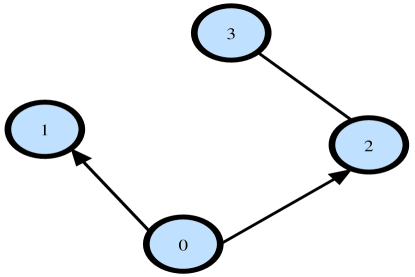
Figure 1: The communication topology graph.

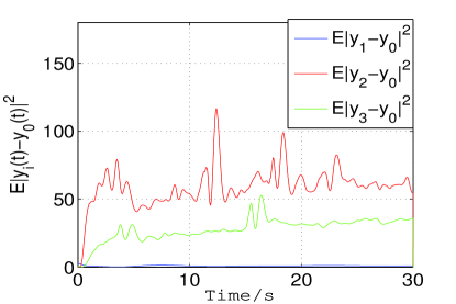
Figure 2: Mean square output tracking errors.

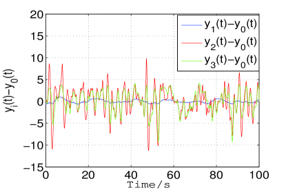
Figure 3: Sample paths of output tracking errors.

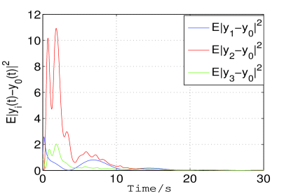
Figure 4: Mean square output tracking errors without
additive noises.

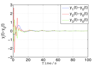
Figure 5: Sample paths of output tracking errors without additive noises.

It can be verified that the pair $(A_{i},B_{i})$ is controllable for $i=1,2,3$, and the pair $(C_{i},A_{i})$ is observable for $i=0,1,2,3$.

Choose $K_{11}=\begin{bmatrix}-10&8&6&12\\ -10&-3&-6&-3\end{bmatrix}$, $K_{12}=K_{13}=\begin{bmatrix}-12&-10&-2&-3\\ 1&-2&-1&-1\\ 5&-1&0&1\end{bmatrix}$, $H_{1}=\begin{bmatrix}-2\\ -1\\ 2\\ 1\end{bmatrix}$, $H_{2}=H_{3}=\begin{bmatrix}-5\\ -3\\ -4\\ -3\end{bmatrix}$ such that $A_{i}+B_{i}K_{1i}$ and $A_{i}+H_{i}C_{i}$ are Hurwitz for $i=1,2,3$. By $(\ref{a1})$, we have

$\Pi_{1}=\begin{bmatrix}1&0&0\\ 2.8072&-1.4746&-2.2583\\ 11.3945&0.1118&0.7853\\ 0.5721&-0.0952&-0.0668\end{bmatrix}$, $\Pi_{2}=\Pi_{3}=\begin{bmatrix}1&0&0\\ 36.6879&14.2062&10.8173\\ -60.6086&1.4485&3.4095\\ 1.3468&-0.6584&-0.6428\end{bmatrix}$, $\Gamma_{1}=\begin{bmatrix}-7.9039&-0.1823&0.1666\\ 1&0&0\end{bmatrix}$, $\Gamma_{2}=\Gamma_{3}=\begin{bmatrix}-6.0891&0.0582&0.2688\\ 1&0&0\\ 1&0&0\end{bmatrix}$. Since $\lambda_{0}^{u}(A_{0})=$
$\sum\limits_{i=1}^{3}\max\{\mathbb{R}\mathbbm{e}(\lambda_{i}(A_{0})),$ $0\}=0.0486$, we select $\alpha=0.65$, $k_{1}=0.38$ and $k_{2}=0.3$.

The mean square errors of sideslip angle and sample paths of sideslip angle errors under the distributed control law $(\ref{b3})$, $(\ref{b4})$ and $(\ref{1})$ are shown in Fig. 2 and Fig. 3. If there are no additive measurement noises, i.e. $\Upsilon_{01}=\Upsilon_{02}=\Upsilon_{23}=\Upsilon_{32}=0$, then mean square errors of sideslip angle and sample paths of sideslip angle errors are shown in Fig. 4 and Fig. 5.

Fig. 2 together with Fig. 4 shows that additive measurement noises lead to a non-zero mean square tracking error while multiplicative measurement noises have no impact on the mean square tracking error. Fig. 5 shows that multiplicative measurement noises make the sample paths of sideslip angle errors fluctuate greatly at the beginning and then vanish. Fig. 3 shows that additive measurement noises make the sample paths of sideslip angle errors fluctuate during the entire process.

V Conclusion

In this paper, we have studied cooperative output feedback tracking control of stochastic linear heterogeneous leader-following multi-agent systems. By output regulation theory and stochastic analysis, we have shown that for observable leader’s dynamics and stabilizable and detectable followers’ dynamics, if (i) the associated output regulation equations are solvable, (ii) the intensity coefficient of multiplicative noises multiplied by the sum of real parts of unstable eigenvalues of the leader’s dynamics is less than $1/4$ of the minimum non-zero eigenvalue of graph Laplacian, then there exist admissible distributed observation and cooperative control strategies based on the certainty equivalent principle to ensure mean square bounded output tracking. Especially, if there are no additive measurement noises, then there exist admissible distributed observation and cooperative control strategies to achieve mean square output tracking. There are still many other interesting topics to be studied in future. Efforts can be made to investigate the consensus problem of HMASs under Markovian switching topologies and HMASs with delays.

Appendix A Definitions and Lemmas

Definition 2

([Mao33], Itô’s formula) Let $x(t)$ be a $d$-dimensional Itô process on $t\geq 0$ with the stochastic differential

$$dx(t)=f(t)dt+g(t)\textrm{d}w(t),$$

where $f\in\mathcal{L}^{1}(\mathbb{R}_{+};\mathbb{R}^{d})$ and $g\in\mathcal{L}^{2}(\mathbb{R}_{+};\mathbb{R}^{d\times m})$. Let $V\in C^{2,1}(\mathbb{R}^{d}\times\mathbb{R}_{+};\mathbb{R})$. Then $V(x(t),t)$ is also an Itô process with the stochastic differential given by

$$\textrm{d}V(x(t),t)= \left[V_{t}(x(t),t)+V_{x}(x(t),t)f(t)+\frac{1}{2}Tr(g^{\rm T}(t)V_{xx}(x(t),t)g(t))\right]\textrm{d}t+V_{x}(x(t),t)g(t)\textrm{d}w(t).$$

Proof of Lemma 1: By Assumption 3, we know that $\left(A_{0}^{\rm T},C_{0}^{\rm T}\right)$ is controllable. If $\mathbb{R}\mathbbm{e}(\lambda_{n}(A_{0}))\geqslant 0$ holds, we choose $\alpha>\lambda_{0}^{u}(A_{0})$. By Lemma 3.1 in [Zong586], we know that $A^{\rm T}P+PA-2\alpha PB\left(I_{p}+B^{\rm T}PB\right)^{-1}$
$B^{\rm T}P+I_{n}=0$ has a unique positive solution $P$, where $A=A_{0}^{\rm T}$ and $B=C_{0}^{\rm T}$. If $\mathbb{R}\mathbbm{e}(\lambda_{n}(A_{0}))<0$ holds, we choose $\alpha=\lambda_{0}^{u}(A_{0})=0$. Therefore, we know that the equation $(\ref{a0})$ is a Lyapunov equation and it has a unique positive solution $P$. $\hfill\square$

Lemma 2

([LiW.Q.]) If $A$ is Hurwtiz, then the solution of the system

$$\textrm{d}x(t)=Ax(t)\textrm{d}t+B\textrm{d}w(t)$$

satisfies

$$\lim_{t\rightarrow\infty}\mathbb{E}\left[\left\|x(t)\right\|^{2}\right]={\rm{Tr}}\left\{\int_{0}^{\infty}e^{As}BB^{T}e^{A^{T}s}\textrm{d}s\right\}.$$

Lemma 3

Denote the matrix $S_{2ij}=[s_{kl}]_{N\times N}$ satisfying

$$\left\{\begin{array}[]{l}s_{kl}=-a_{ij},\quad k=i,l=i,\\[5.0pt] s_{kl}=a_{ij},\quad k=i,l=j,\\[5.0pt] s_{kl}=0,\quad otherwise,\end{array}\right.$$ (15)

then $\sum\limits_{i,j=1}^{N}\left({S_{2ij}^{\rm T}}S_{2ij}\right)=2\mathcal{L}$, where $\mathcal{L}$ is the Laplacian matrix of $\mathcal{G}$, $\mathcal{A}$ is the adjacency matrix of $\mathcal{G}$ and $a_{ij}$ is the element of $\mathcal{A}$.

Proof : By the definition of $S_{2ij}$, $1\leqslant i\leqslant j\leqslant N$, we have

$$S_{2ij}=\bordermatrix{&1&\quad&i&\quad&j&\quad\cr 1&0&\cdots&0&\cdots&0&\cdots\cr\quad&\vdots&\cdots&\vdots&\cdots&\vdots&\cdots\cr i&0&\cdots&-a_{ij}&\cdots&a_{ij}&\cdots\cr&\vdots&\cdots&\vdots&\cdots&\vdots&\cdots\cr j&0&\cdots&0&\cdots&0&\cdots\cr&\vdots&\cdots&\vdots&\cdots&\vdots&\cdots\cr}_{N\times N},$$

where the omitted elements are zero.

By the above equation, we obtain

$$S_{2ij}^{\rm T}S_{2ij}=\bordermatrix{&1&\quad&i&\quad&j&\quad\cr 1&0&\cdots&0&\cdots&0&\cdots\cr\quad&\vdots&\cdots&\vdots&\cdots&\vdots&\cdots\cr i&0&\cdots&a_{ij}^{2}&\cdots&-a_{ij}^{2}&\cdots\cr&\vdots&\cdots&\vdots&\cdots&\vdots&\cdots\cr j&0&\cdots&-a_{ij}^{2}&\cdots&a_{ij}^{2}&\cdots\cr&\vdots&\cdots&\vdots&\cdots&\vdots&\cdots\cr}_{N\times N}.$$

By $a_{ij}=0$ or $a_{ij}=1$, we have $a_{ij}^{2}=a_{ij}$, which together with the above equation gives

$$S_{2ij}^{\rm T}S_{2ij}=\bordermatrix{&1&\quad&i&\quad&j&\quad\cr 1&0&\cdots&0&\cdots&0&\cdots\cr\quad&\vdots&\cdots&\vdots&\cdots&\vdots&\cdots\cr i&0&\cdots&a_{ij}&\cdots&-a_{ij}&\cdots\cr&\vdots&\cdots&\vdots&\cdots&\vdots&\cdots\cr j&0&\cdots&-a_{ij}&\cdots&a_{ij}&\cdots\cr&\vdots&\cdots&\vdots&\cdots&\vdots&\cdots\cr}_{N\times N}.$$

Correspondingly, for $1\leqslant j\leqslant i\leqslant N$, we get