Posterior asymptotics in Wasserstein metrics on the real line

Abstract

In this paper, we use the class of Wasserstein metrics to study asymptotic properties of posterior distributions. Our first goal is to provide sufficient conditions for posterior consistency. In addition to the well-known Schwartz’s Kullback–Leibler condition on the prior, the true distribution and most probability measures in the support of the prior are required to possess moments up to an order which is determined by the order of the Wasserstein metric. We further investigate convergence rates of the posterior distributions for which we need stronger moment conditions. The required tail conditions are sharp in the sense that the posterior distribution may be inconsistent or contract slowly to the true distribution without these conditions. Our study involves techniques that build on recent advances on Wasserstein convergence of empirical measures. We apply the results to some examples including a Dirichlet process mixture prior and conduct a simulation study for further illustration.

and

1 Introduction

The Wasserstein distance originally arose in the problem of optimal transportation [43] and is often called the Kantorovich or transportation distance. We refer to [42] for the history about this metric. For two Borel probability measures $P$ and $Q$ on the real line, the Wasserstein metric of order $p$, $p\in[1,\infty)$, is defined as

$$W_{p}(P,Q)=\inf_{\pi\in{\mathscr{C}}(P,Q)}\left(\int_{{\mathbb{R}}^{2}}|x-y|^{p}d\pi(x,y)\right)^{1/p},$$

where ${\mathscr{C}}(P,Q)$ is the set of every coupling $\pi$ of $P$ and $Q$, that is, a Borel probability measure on ${\mathbb{R}}^{2}$ with marginals $P$ and $Q$, respectively.

There are a wide number of applications of Wasserstein metrics, e.g. Wasserstein generative adversarial networks (GAN; [1, 25]), approximate Markov chain Monte Carlo (MCMC; [38]), distributionally robust optimization (DRO; [31]) and clustering ([4, 32]). However, exhaustive study on statistical properties such as the convergence behavior of the empirical measure with respect to $W_{p}$ have been conducted only recently, see [7, 18, 46, 15]. In particular, the great success of Wasserstein GAN in machine learning society accelerated the study of Wasserstein metrics in statistics community as a discrepancy measure between probabilities; [41, 34, 5]. Recently, [3] proposed the use of the Wasserstein distance in the implementation of Approximate Bayesian Computation (ABC) to approximate the posterior distribution. In nonparametric Bayesian inference, [36, 12] used Wasserstein metrics to study asymptotic properties of posterior distributions, but $W_{p}$ was considered as a distance between mixing distributions rather than a distance between mixture densities themselves. As a result, the Wasserstein metrics in these papers yielded a stronger topology than the total variation distance on the space of density functions. In general, $W_{p}$, $1\leq p<\infty$, metrizes the weak convergence of probability measures in a bounded metric space. Specifically, if the diameter of the underlying metric space is bounded by 1, one has the relationship $d_{P}^{2}\leq W_{1}\leq 2d_{P}\leq d_{V}$, where $d_{P}$ and $d_{V}$ are Lévy-Prokhorov and total variation distances, see [23]. In an unbounded metric space, the second and third inequalities do not hold because $W_{1}$ is not a bounded metric.

In this article, we utilize the Wasserstein distances to study asymptotic behavior of posterior distributions under the assumption that data are generated from a fixed true distribution and we focus on nonparametric Bayesian density estimation on the real line. To set the stage, let $X_{1},\ldots,X_{n}$ be the observations which are independent and identically distributed random variables from the true distribution $P_{0}$ possessing a density $p_{0}$. Let $\mathcal{F}$ be a collection of probability densities in ${\mathbb{R}}$ equipped with the weak topology, and $\Pi$ be a prior distribution on $\mathcal{F}$. Then the posterior probability of a measurable set $A\subset\mathcal{F}$ is given as

$$\Pi(p\in A\mid X_{1},\ldots,X_{n})=\frac{\int_{A}\prod_{i=1}^{n}p(X_{i})/p_{0}(X_{i})d\Pi(p)}{\int\prod_{i=1}^{n}p(X_{i})/p_{0}(X_{i})d\Pi(p)}$$ (1.1)

by the Bayes formula. Throughout the paper, we allow the prior $\Pi$ to depend on the sample size $n$, but often abbreviate this dependency in the notation of both prior and posterior distributions. If clarification is necessary, the prior and posterior will be denoted $\Pi_{n}$ and $\Pi_{n}(\cdot\mid X_{1},\ldots,X_{n})$, respectively. The posterior distribution is said to be consistent with respect to a (pseudo-)metric $d$ if

$$\Pi\Big{(}d(p,p_{0})>\epsilon\mid X_{1},\ldots,X_{n}\Big{)}\rightarrow 0~{}\text{in probability for every $\epsilon>0$},$$

where the convergence in probability is taken with respect to the true distribution $P_{0}$. If $\epsilon$ is replaced by $\epsilon_{n}$ for some sequence $\epsilon_{n}\rightarrow 0$, the convergence rate of the posterior distributions is said to be at least $\epsilon_{n}$. There is a huge amount of research articles concerning asymptotic properties of the posterior distribution. We refer to the monograph [22] for the history and details about this topic.

Of key importance is the Kullback–Leibler (KL) support condition developed by [39]. A fixed prior $\Pi$ is said to satisfy the KL support condition if

$$\Pi\Big{(}p:K(p_{0},p)<\epsilon\Big{)}>0\quad\text{for every $\epsilon>0$},$$ (1.2)

where $K(p_{0},p)=\int\log[p_{0}(x)/p(x)]dP_{0}(x)$ is the KL divergence. If the prior depends on the sample size, the KL condition (1.2) can be replaced by

$$\liminf_{n\rightarrow\infty}\Pi_{n}\Big{(}p:K(p_{0},p)<\epsilon\Big{)}>0\quad\text{for every $\epsilon>0$}.$$ (1.3)

Conditions (1.2) and (1.3) became standard for proving posterior consistency. In particular, it gives a suitable lower bound of the denominator in (1.1) and it implies posterior consistency in the weak topology, that is with respect to the Lévy-Prokhorov distance, see [39] and Section 6.4 of [22]. A variation of the KL support condition to obtain a convergence rate is developed by [20]. It is formally expressed as

$$\Pi(\mathcal{K}_{n})\geq e^{-n\epsilon_{n}^{2}}\quad\text{for all large enough $n$,}$$ (1.4)

where

$$\mathcal{K}_{n}=\left\{p\in\mathcal{F}:\int\log\frac{p_{0}}{p}dP_{0}\leq\epsilon_{n}^{2},\int\Big{(}\log\frac{p_{0}}{p}\Big{)}^{2}dP_{0}\leq\epsilon_{n}^{2}\right\}.$$

In literature, studies on posterior asymptotics have focused on strong metrics such as the total variation, Hellinger and uniform metrics. For those purposes, some non-trivial conditions such as the bounded entropy or prior summability are assumed in addition to the KL conditions, see [19, 45, 2, 11] for example. On the other hand, it is surprising that careful analysis of the convergence rates with respect to a weak metric such as the Lévy-Prokhorov and Kolmogorov has not been studied in literature, considering that the KL support condition is sufficient for the consistency in those metrics. [11] studied the convergence rate of the posterior distribution with respect to the Lévy-Prokhorov metric, but their rate $n^{-1/4}$ have a lot of room for improvement. Furthermore, they used the Lévy-Prokhorov rate as a tool for proving the consistency in total variation, and did not focus on the convergence rate itself.

Wasserstein metrics $W_{p}$, $1\leq p<\infty$ metrize weak convergence in a bounded space, but it generates a stronger topology in general. Indeed, neither the KL support condition (1.2) nor (1.4) are sufficient for posterior consistency with respect to $W_{p}$. If $P_{0}$ is a standard Cauchy density, for example, $W_{p}(P,P_{0})=\infty$ for any $P$ and $p\geq 1$. Therefore, for any prior except the one putting all its mass on $P_{0}$, the posterior distribution is inconsistent with respect to $W_{p}$. This simple example shows that tails or moments of probability measures play an important role for handling $W_{p}$.

For a sequence $P_{n}$ of probability measures, it is well-known that $W_{p}(P_{n},P)\rightarrow 0$ if and only if $P_{n}$ converges to $P$ weakly and $M_{p}(P_{n})\rightarrow M_{p}(P)$, see [43], p.212, where $M_{p}(P)=\int|x|^{p}dP(x)$. Therefore, for the Wasserstein consistency to hold, the posterior moment should converge to the true moment, see Theorem 2.1. However, while the moment consistency of frequentist’s nonparametric estimators such as the the empirical distribution is straightforward, it is non-trivial to show that the posterior moment converges to the true moment even with a very popular prior such as a Dirichlet process mixture. This is mainly because tails of probability measures in the support of the prior should be considered simultaneously.

To prove posterior consistency, we will leverage on the KL condition. We provide two different approaches which are of independent interest; see the proof of Theorem 2.2. The first one targets directly posterior moment consistency and relies on a result from [45]. The second one has less stringent conditions but the proof is more complicated. Specifically, we construct uniformly consistent tests based on the empirical distribution by exploiting suitable upper bounds of Wasserstein metrics. We then show that, to achieve posterior consistency with respect to $W_{p}$, moments of densities must be suitably bounded. In particular, the posterior needs to put most of its mass on distributions that possess moments up to an order determined by that of the Wasserstein metric. In practice, the posterior moment condition can be worked out by means of exponentially small prior probability on the complement set, cf. Lemma 8.2. In Section 5.2 we provide an illustration in the specific example of Dirichlet process mixture prior.

Both approaches for posterior consistency can be extended to obtain suitable convergence rates with the KL condition (1.4). While the first approach gives the convergence rate for the moment, the second approach gives the rate with respect to $W_{p}^{p}$ relying on slightly stronger moment conditions, see Theorems 3.1 and 3.2. For convergence rates with the second approach, we rely on new upper bounds on Wasserstein metrics that can be of independent interest, cf. Lemma 8.7. Interestingly, the posterior moment conditions for consistency and convergence rates are nearly necessary, that is the posterior distribution may be inconsistent or contract slowly to the true distribution when they are not satisfied. Finally, we obtain convergence rates for the case $p=\infty$ in Theorem 4.1, for which we need to restrict to probability measures on a bounded space.

To the best of our knowledge, this paper is the first result on posterior asymptotics with the Wasserstein metric. The remainder of this paper is organized as follows. Results on posterior consistency and its convergence rate with respect to $W_{p}$, for $1\leq p<\infty$, are considered in Sections 2 and 3, respectively. Posterior asymptotics with respect to $W_{\infty}$ is studied in Section 4. Section 5 considers more details with specific examples. Some numerical results complementing our theory are provided in Section 6. Concluding remarks and proofs are given in Sections 7 and 8, respectively.

Notation

Before proceeding, we introduce some further notation; for two real numbers $a$ and $b$, their minimum and maximum are denoted by $a\wedge b$ and $a\vee b$, respectively. Inequality $a\lesssim b$ means that $a$ is less than a constant multiple of $b$, where the constant is universal unless specified. Upper cases such as $P$ and $Q$ refer to probability measures corresponding to the densities denoted by lower cases and vise versa. The empirical measure based on $X_{1},\ldots,X_{n}$ is denoted ${\mathbb{P}}_{n}$. For a real-valued function $f$, its expectation with respect to $P$ is denoted $Pf$. The expectation with respect to the true distribution is often denoted $\mathrm{E}f(X)$. The restriction of $P$ onto a set $A$ is denoted $P|_{A}$.

2 Consistency with respect to $W_{p}$

Recall that $W_{p}(P_{n},P)\rightarrow 0$ if and only if $P_{n}$ converges weakly to $P$ and $M_{p}(P_{n})\rightarrow M_{p}(P)$, see Theorem 7.12 of [43]. Also, the KL support condition (1.2), or (1.3), guarantees posterior consistency with respect to the Lévy-Prokhorov metric which induces the weak convergence. Therefore, it is natural under the KL support condition to guess that posterior consistency with respect to $W_{p}$ is equivalent to the consistency of the $p$th moment, that is,

$$\Pi\Big{(}\big{|}M_{p}(P)-M_{p}(P_{0})\big{|}>\epsilon\mid X_{1},\ldots,X_{n}\Big{)}\rightarrow 0\quad\text{in probability for every $\epsilon>0$.}$$ (2.1)

If (2.1) holds, we say that the posterior moment of order $p$ is consistent. For $p=1$, the moment consistency can be easily implied by $W_{1}$-consistency by the help of the duality theorem by [30], see also [17, 14, 44], which asserts that

$$W_{1}(P,Q)=\sup_{f\in{\mathscr{L}}}\left|\int f(x)dP(x)-\int f(x)dQ(x)\right|,$$

where ${\mathscr{L}}$ is the class of every Lipschitz function whose Lipschitz constant is bounded by 1. Since the map $x\mapsto|x|$ belongs to ${\mathscr{L}}$, we have that $\left|M_{1}(P)-M_{1}(Q)\right|\leq W_{1}(P,Q).$ Although such an explicit bound does not exist for $p>1$, one can show that posterior consistency with respect to the Wasserstein distance is equivalent to the moment consistency under the KL support condition.

Theorem 2.1.

For a prior $\Pi$, suppose that the KL condition (1.3) holds. Then, the consistency of the $p$-th moment (2.1) is equivalent to that

$$\Pi\Big{(}W_{p}(P,P_{0})\geq\epsilon\mid X_{1},\ldots,X_{n}\Big{)}\longrightarrow 0\quad\text{in probability for every $\epsilon>0$}.$$ (2.2)

We provide two different approaches for proving posterior consistency with respect to $W_{p}$ which are of independent interests. The first approach relies on a result from [45]; namely that if $\mathcal{C}$ is a convex set of probability measures and $\inf_{P\in\mathcal{C}}H(P_{0},P)>0$ then $\Pi(\mathcal{C}|X_{1},\ldots,X_{n})\to 0$ in probability, where $H(P,Q)$ denotes the Hellinger distance between $P$ and $Q$. This approach directly uses Theorem 2.1 by establishing the consistency of the $p$th moment (2.1). The proof based on this approach is very simple as it only needs a single application of the Cauchy–Schwarz inequality. However, it requires the moment of order $2p$ to be bounded a posteriori.

The second approach constructs a uniformly consistent sequence of tests based on the convergence of empirical distribution. The uniformity does not make any problem for the compact support case, i.e. $P_{0}([-1,1])=1$ and $P([-1,1])=1$ for every $P$ in the support of the prior $\Pi$. If probability measures in the support of the prior have unbounded support, however, problems may happen due to probability measures with large moments. This problem can be avoided if the moments are suitably bounded a posteriori, as expressed through condition (2.3) below. The second approach relies on a rather complicated proof, but it only needs the moment of order $p+\delta$, for some $\delta>0$, to be bounded.

Theorem 2.2.

Assume that the prior $\Pi$ satisfies the KL condition (1.3). Furthermore, assume that there exist positive constants $K$ and $\delta$ such that $M_{p+\delta}(P_{0})<\infty$ and

$$\Pi\Big{(}M_{p+\delta}(P)\leq K\mid X_{1},\ldots,X_{n}\Big{)}\rightarrow 1~{}\text{in probability.}$$ (2.3)

Then for every $\epsilon>0$,

$$\Pi\Big{(}W_{p}(P,P_{0})>\epsilon\mid X_{1},\ldots,X_{n}\Big{)}\longrightarrow 0~{}\text{in probability}.$$

It should be emphasized that assumptions in Theorem 2.2 are nearly necessary. Certainly, $M_{p}(P_{0})<\infty$ is necessary. Since the consistency with respect to $W_{p}$ entails the consistency of the $p$th moment by Theorem 2.1, it is also necessary that

$$\Pi\Big{(}M_{p}(P)\leq K\mid X_{1},\ldots,X_{n}\Big{)}\rightarrow 1\quad\text{in probability for some constant $K$.}$$ (2.4)

On the other hand, $M_{p}(P_{0})<\infty$ and (2.4) are not sufficient for the posterior distribution to be consistent with respect to $W_{p}$, as shown in the following example.

Example.

Let $P_{0}=\delta_{0}$, $P_{n}=(1-n^{-1})\delta_{0}+n^{-1}\delta_{x_{n}}$ and $\Pi(\{P_{0}\})=\Pi(\{P_{n}\})=1/2$, where $\delta_{x}$ is the Dirac measure at $x$ and $x_{n}=n^{1/p}$. Obviously, the KL condition (1.3) holds. Furthermore, $W_{p}^{p}(P_{0},P_{n})=M_{p}(P_{n})=1<\infty$ and $M_{p+\delta}(P_{n})=n^{\delta/p}\rightarrow\infty$ for every $\delta>0$. Since $P_{0}(X_{1}=0,\ldots,X_{n}=0)=1$ and $P_{n}(X_{1}=0,\ldots,X_{n}=0)=(1-n^{-1})^{n}\rightarrow e^{-1}>0$, the posterior distribution is inconsistent with respect to $W_{p}$. Here, condition (2.4) holds, but (2.3) is violated for any $\delta>0$.

By Theorem 2.2, the proof of the Wasserstein consistency boils down to

$$\Pi\Big{(}M_{p}(P)\leq K\mid X_{1},\ldots,X_{n}\Big{)}\longrightarrow 1\quad\text{in probability}$$ (2.5)

for a constant $K$, a condition that seems easy to prove at first sight. However, the proof is not simple even with a well-known prior which puts all of its mass on the space of light-tailed distributions, that is, distribution with large or infinite tail index. Here, if a distribution function $F$ satisfies $1-F(x)=x^{-\alpha}L(x)$ for large enough $x$, where $L(\cdot)$ is a slowly varying function satisfying $\lim_{y\rightarrow\infty}L(xy)/L(y)=1$ for any $x>0$, the positive constant $\alpha$ is called the (right) tail index of $F$, see [33] for a Bayesian consistency of the tail index. It should be noted that a light-tail, i.e. large tail index, does not guarantee a small value of moment, which makes the proof of posterior consistency in $W_{p}$ difficult. This is in stark contrast to that the moment of the empirical distribution can be trivially shown to be consistent. In Section 5.2, we are able to work out the case of Dirichlet process mixture prior by using Lemma 8.2, that is by establishing that the prior puts exponentially small mass to probability measures $P$ with $M_{p}(P)>K$. See Theorem 5.1.

3 Convergence rates with respect to $W_{p}$

For a given rate sequence $\epsilon_{n}$, suppose that $\Pi(\mathcal{K}_{n})\geq e^{-n\epsilon_{n}^{2}}$ for every large enough $n$. Based on this condition, which is used to find a lower bound of the integrated likelihood, the denominator in the expression (1.1), we will extend the results of Section 2 to obtain a convergence rate. The main task in this section is to find additional assumptions required to achieve the convergence rate $\epsilon_{n}$. An extension of the first proof for Theorem 2.2 requires the moment of order $2p$ as follows.

Theorem 3.1.

Assume that the prior $\Pi$ satisfies the KL condition (1.4) for a sequence $\epsilon_{n}$ with $\epsilon_{n}\to 0$ and $n\epsilon_{n}^{2}\to\infty$. Furthermore, assume that there exists a constant $K$ such that $M_{2p}(P_{0})\leq K$ and

$$\Pi\Big{(}P:\,M_{2p}(P)>K\mid X_{1},\ldots,X_{n}\Big{)}\to 0\quad\text{in probability.}$$

Then

$$\Pi\Big{(}|M_{p}(P)-M_{p}(P_{0})|>K^{\prime}\epsilon_{n}\mid X_{1},\ldots,X_{n}\Big{)}\to 0\quad\text{in probability}$$

for some constant $K^{\prime}>0$.

Note that $M_{p}(P)$ is a linear functional of $P$ for which the semi-parametric Bernstein–von Mises (BvM) theorem may hold, see [9, 37]. In this case, the convergence rate of the marginal posterior distribution of $M_{p}(P)$ would be the parametric rate $n^{-1/2}$ even though the global posterior convergence rate $\epsilon_{n}$ may be slower. However, while Theorem 3.1 is very general, the semi-parametric BvM theorem holds under rather strong conditions. For example, the above mentioned papers consider only specific priors and relied on the assumption that $p_{0}$ is compactly supported and bounded away from zero. It is sometimes possible to obtain the parametric convergence rate for the finite-dimensional parameter of interests without the semi-parametric BvM theorem. However, the proof typically relies on the LAN (locally asymptotically normal) expansion of the log-likelihood, see [6, 10].

Next, we consider an extension of the testing approach. To achieve the convergence rate $\epsilon_{n}$, we will construct a sequence of consistent test

$$P_{0}\phi_{n}\rightarrow 0\quad{\rm and}\quad\sup_{P\in\mathcal{F}_{n}^{c}}P(1-\phi_{n})\leq e^{-3n\epsilon_{n}^{2}},$$

where $\mathcal{F}_{n}=\{P:W_{p}^{p}(P,P_{0})\leq K\epsilon_{n}\}\cap\mathcal{F}_{0}$. Here, $\mathcal{F}_{0}$ will be defined as a collection of probability measures whose tails and moments are suitably bounded. Then, it will suffices for the desired result to show that $\Pi(\mathcal{F}_{0}^{c}\mid X_{1},\ldots,X_{n})\rightarrow 0$ in probability.

A consistent sequence of tests will be constructed based on the convergence of the empirical distribution to the true distribution. Note that there are well-known concentration inequalities of the form $P(W_{p}^{p}({\mathbb{P}}_{n},P)>\epsilon_{n})\leq\delta_{n},$ where $\delta_{n}$ is a decaying sequence, and those inequalities might be directly used to define tests as

$$\phi_{n} = \left\{\begin{array}[]{ll}1&~{}~{}\text{if $W_{p}^{p}({\mathbb{P}}_{n},P_{0})>\epsilon_{n}$}\\ 0&~{}~{}\text{otherwise.}\end{array}\right.$$

However, such a simple approach does not give sharp convergence rates of the posterior distribution. For example, if we apply the concentration inequality by [18], for any $P$ with $W_{p}^{p}(P,P_{0})>2^{p}\epsilon_{n}$ and $M_{2p+\delta}(P)<\infty$, we have

$$\begin{split}&P(1-\phi_{n})=P\Big{(}W_{p}^{p}({\mathbb{P}}_{n},P_{0})\leq\epsilon_{n}\Big{)}\leq P\Big{(}W_{p}^{p}({\mathbb{P}}_{n},P)\geq 2^{-(p-1)}W_{p}^{p}(P,P_{0})-\epsilon_{n}\Big{)}\\ &\leq P\Big{(}W_{p}^{p}({\mathbb{P}}_{n},P)\geq\epsilon_{n}\Big{)}\leq c_{1}\bigg{(}e^{-c_{2}n\epsilon_{n}^{2}}+\frac{1}{n\epsilon_{n}^{2}}\frac{1}{(n\epsilon_{n})^{\delta/2p}}\bigg{)}\end{split}$$ (3.2)

where $c_{1}$ and $c_{2}$ are constants. Here, the constants $c_{1}$ and $c_{2}$ depends on the moments of $P$, so it is not easy to bound (LABEL:eq:concentration-ineq) uniformly. Furthermore, the second term in the right hand side of (LABEL:eq:concentration-ineq) is of polynomial order in $n\epsilon_{n}^{2}$ which decays too slowly compared to $e^{-n\epsilon_{n}^{2}}$. In turn, the use of $\phi_{n}$ would give a much slower convergence rate than $\epsilon_{n}$.

Theorem 3.2 below is our main results concerning convergence rates of the posterior distribution. Proof of Theorem 3.2 relies on the set-up in [18]. In particular, Lemmas 8.3 and 8.5 can be easily deduced from the results in [18]. We build on these two lemmas to develop some techniques whose details are different from [18]. As mentioned above, we need to construct a sequence of tests decaying with an exponential rate. As far as we know, this is not possible with the proof technique used in [18]. Given a bounded moment condition, we achieve this by the help of Lemma 8.7. The condition $\epsilon_{n}\geq\sqrt{(\log n)/n}$ in Theorem 3.2 is assumed only for technical reason. Although we could not succeed to eliminate this condition, we believe the result is valid for any $\epsilon_{n}\downarrow 0$ with $n\epsilon_{n}^{2}\rightarrow\infty$.

Theorem 3.2.

Assume that the prior $\Pi$ satisfies the KL condition (1.4) for a sequence $\epsilon_{n}$ with $\epsilon_{n}\downarrow 0$ and $\epsilon_{n}\geq\sqrt{(\log n)/n}$. Furthermore, assume that there exist positive constants $K$ and $\delta$ such that $M_{2p+\delta}(P_{0})<\infty$ and $\Pi(M_{2p+\delta}(P)\leq K\mid X_{1},\ldots,X_{n})\rightarrow 1$ in probability. Then, for some constant $K^{\prime}>0$,

$$\Pi\Big{(}W_{p}^{p}(P,P_{0})\geq K^{\prime}\big{\{}\epsilon_{n}+I(p=1)\log\epsilon_{n}^{-1}\big{\}}\mid X_{1},\ldots,X_{n}\Big{)}\longrightarrow 0\quad\text{in probability}.$$

Assumptions in Theorems 3.2 should be understood as sufficient conditions so that $\Pi(\mathcal{K}_{n})\geq e^{-n\epsilon_{n}^{2}}$ guarantees $\epsilon_{n}$ as the posterior convergence rate for any $\epsilon_{n}\gg n^{-1/2}$. For the empirical measure to achieve the rate $n^{-1/2}$ with respect to $W_{p}^{p}$, the same moment condition $M_{2p+\delta}(P_{0})<\infty$ is considered in [18]. They provided an example showing that this moment condition cannot be weakened in general. As illustrated in the example at the end of this section, the posterior moment condition $\Pi(M_{2p+\delta}(P)\leq K\mid X_{1},\ldots,X_{n})\rightarrow 1$ cannot also be weakened.

When $p>1$, Theorem 3.2 gives a rate $\epsilon_{n}$ with respect to $W_{p}^{p}$ rather than $W_{p}$. This result is more relevant to [18] than [7]. In particular, condition $M_{2p+\delta}(P_{0})<\infty$ is the same to Eq. (3) of [18], and much weaker than

$$\int\frac{[F_{0}(x)(1-F_{0}(x))]^{p/2}}{p_{0}(x)^{p-1}}dx<\infty$$ (3.3)

which is a necessary and sufficient condition in [7] for that $\mathrm{E}[W_{p}({\mathbb{P}}_{n},P_{0})]\asymp n^{-1/2}$. When $p=1$, $M_{2p+\delta}(P_{0})<\infty$ is only slightly stronger than (3.3), which is reduced to $\int\sqrt{F_{0}(x)(1-F_{0}(x))}dx<\infty$, where $F_{0}$ is the cumulative distribution function of $P_{0}$. If $p>1$, however, $M_{2p+\delta}(P_{0})<\infty$ is much weaker than (3.3) which may not be satisfied even when $P_{0}$ is compactly supported. Note that if $P_{0}$ is standard normal, (3.3) is satisfied if and only if $1\leq p<2$. As mentioned in [7], the rate $\mathrm{E}[W_{p}({\mathbb{P}}_{n},P_{0})]\asymp n^{-1/2}$ cannot be obtained under moment-type conditions considered in Theorem 3.2. Therefore, we would need a stronger assumption such as (3.3) to replace $W_{p}^{p}$ by $W_{p}$ in Theorem 3.2. Since we are focusing on the moment-type condition in the present paper, we do not address more detail about condition (3.3). Instead, we consider the metric $W_{\infty}$ in Section 4 with a stronger assumption. Specifically, $P_{0}$ will be assumed to be supported on a bounded interval. This is necessary to obtain the consistency with respect to $W_{\infty}$. The result in Section 4 guarantees the rate $\epsilon_{n}$ with respect to $W_{p}$, not $W_{p}^{p}$, at least when probabilities are compactly supported.

Note that our approach does not guarantee the rate $n^{-1/2}$ which is minimax optimal and achieved by the empirical measure under some general conditions, e.g. [47, 18, 7]. Our approach gives the rate $n^{-1/2}$ only if the prior puts sufficiently large mass around the KL neighborhood of $p_{0}$. This is mainly because our approach relies on the general approach of [20] for which the KL condition $\Pi(\mathcal{K}_{n})\gtrsim e^{-n\epsilon_{n}^{2}}$ plays an important role to determine the rate. Also, note that the testing approach only gives sharp rates when the distance is compatible with the natural statistical distance of the model, the Hellinger distance in our case, see [27] for extensive discussion on this point. In this regards, it might not be possible to obtain sharp rates based on the testing approach. Hence, a different approach would be necessary to achieve the rate $n^{-1/2}$, e.g. the approach in [27, 48]. Another possible approach would be to utilize the functional Bernstein–von Mises theorem. Specifically, the approach given in [8], combining with the Kantorovich-Rubinstein representation, might give the rate $n^{-1/2}$ at least for $W_{1}$, and further limiting distribution of the posterior distribution. Note that the above papers are limited to specific priors and probability measures on a bounded set, while the present paper focuses on the moment condition for the posterior convergence rate. With these approaches, it would be highly interesting to investigate sufficient conditions to achieve the rate $n^{-1/2}$.

For $p=1$, an additional logarithmic term in Theorem 3.2 can be eliminated if we assume a slightly stronger condition, which is satisfied if $p_{0}(x)\leq K|x|^{-(3+\delta)}$ and $\Pi(p(x)\leq K|x|^{-(3+\delta)}~{}\forall x\mid X_{1},\ldots,X_{n})\rightarrow 1$ in probability for some positive constants $K$ and $\delta$, see Theorem 8.9 for details. Since Theorem 8.9 relies on some technical assumptions, we defer its statement to Section 8, and provide here a simpler statement, Theorem 3.2. Proofs of these theorems are quite similar.

Finally, we note that moment conditions in Theorem 3.2 cannot be weakened to $\delta<0$ as shown in the following example.

Example.

Let $P_{0}=\delta_{0}$, $P_{n}=(1-n^{-1})\delta_{0}+n^{-1}\delta_{x_{n}}$ and $\Pi(\{P_{0}\})=\Pi(\{P_{n}\})=1/2$. Certainly, the KL condition (1.4) holds for any $\epsilon_{n}\gg n^{-1/2}$. Note that the likelihood given $P_{n}$ equals to $(1-n^{-1})^{n}$ $P_{0}$-almost-surely, which converges to $e^{-1}>0$. If $x_{n}=n^{1/(2p)+\delta}$ for small enough $\delta>0$, then $W_{p}^{p}(P_{0},P_{n})=n^{-(1/2-p\delta)}$. Therefore, the posterior distribution is consistent with respect to $W_{p}^{p}$, but the rate of convergence is strictly slower than $\sqrt{(\log n)/n}$. In this example, note that $\int|x|^{2p}dP_{n}(x)=n^{2\delta p}\rightarrow\infty$, so the posterior moment condition in Theorem 3.2 is not satisfied.

4 Convergence rates with respect to $W_{\infty}$

Since $W_{p}(P,Q)$ monotonically increases in $p$, one may define $W_{\infty}(P,Q)=\lim_{p\rightarrow\infty}W_{p}(P,Q)$ which, according to [24], corresponds to

$$W_{\infty}(P,Q)=\inf\Big{\{}\epsilon>0:P(A)\leq Q(A^{\epsilon}),\;\forall A\in\mathcal{R}\Big{\}},$$

where $A^{\epsilon}=\{x:|x-y|<\epsilon~{}\text{for some}~{}y\in A\}$ is the $\epsilon$-enlargement of $A$ and $\mathcal{R}$ is the set of all Borel subsets of ${\mathbb{R}}$. This representation of $W_{\infty}$ bears similarities with the Lévy-Prokhorov metric

$$d_{P}(P,Q)=\inf\Big{\{}\epsilon>0:P(A)\leq Q(A^{\epsilon})+\epsilon,\;\forall A\in\mathcal{R}\Big{\}}$$

which metrizes the weak convergence.

The metric $W_{\infty}$ induces a much stronger topology than the weak topology even in a bounded metric space. In an unbounded space, if the tail index of two probability measures $P$ and $Q$ are different, then $W_{\infty}(P,Q)$ is typically infinity. For example, if $P$ and $Q$ are Student’s $t$-distributions with $\nu_{1}$ and $\nu_{2}$ degrees of freedom with $\nu_{1}\neq\nu_{2}$, then $W_{\infty}(P,Q)=\infty$. Therefore, it is meaningless to study asymptotics with $W_{\infty}$ in an unbounded space.

In this section, we assume that $P_{0}$ is supported in the unit interval $[0,1]$, and so are all probability measures in the support of the prior. Our benchmarking assumption is $\inf_{x\in[0,1]}p_{0}(x)\geq c_{0}$ for some constant $c_{0}>0$, which is a necessary and sufficient condition for that $P_{0}[W_{\infty}({\mathbb{P}}_{n},P_{0})]\asymp n^{-1/2}$, see [7].

Theorem 4.1.

Suppose that $p_{0}$ is a density on $[0,1]$ and $\inf_{x\in[0,1]}p_{0}(x)\geq c_{0}$ for some constant $c_{0}>0$. Also, assume that the prior $\Pi$ satisfies the KL condition (1.4) for a sequence $\epsilon_{n}$ with $\epsilon_{n}\downarrow 0$ and $\epsilon_{n}\geq\sqrt{(\log n)/n}$ and $\Pi(P([0,1])=1)=1$. Then, for some constant $K>0$,

$$\Pi\bigg{(}W_{\infty}(P,P_{0})>K\epsilon_{n}~{}\Big{|}~{}X_{1},\ldots,X_{n}\bigg{)}\longrightarrow 0\quad\text{in probability}.$$ (4.1)

5 Examples

In this section, we consider the posterior moment condition (2.5) with two examples. In the first example, we illustrate the idea of a novel approach handling the second moment condition without full technical details. The approach relies on a special property of gamma distributions. The second example considers higher order moments, and concrete posterior convergence rates are derived.

Note that (2.5) holds trivially if the prior satisfies

$$\Pi\Big{(}p:p(x)\leq K^{\prime}t_{p}(x)~{}\forall x\Big{)}=1$$ (5.1)

for some $K^{\prime}$, where $t_{p}$ is the density of the Student’s $t$ distribution with $p$ degrees of freedom. Such a prior can be easily constructed by conditioning well-known priors by the event in the left hand side of (5.1). Although the prior probability for this event would be close to 1 with most priors and large enough $K$, this conditioning might be unnatural in practice.

5.1 Mixture of gamma distributions

Suppose it is required to establish weak consistency alongside a functional constraint; such as

$$\Pi\left(p:\int x^{2}p(x)\,dx>K\mid X_{1},\ldots,X_{n}\right)\to 0$$

in probability, for some finite $K>0$, with the prior $\Pi$ on density functions on $(0,\infty)$. This would be for establishing $W_{1}$ consistency.

With the usual Kullback–Leibler support condition, we write the posterior as

$$d\Pi(p\mid X_{1},\ldots,X_{n})=\frac{\prod_{i=1}^{n}\alpha(x_{i})\frac{p(x_{i})}{p_{0}(x_{i})}d\Pi(p)}{\int\prod_{i=1}^{n}\alpha(x_{i})\frac{p(x_{i})}{p_{0}(x_{i})}d\Pi(p)},$$

for some function $\alpha$. Using standard arguments, the $P_{0}$-expectation of the numerator over the set $A$ is

$$\int_{A}\left(\int\alpha dP\right)^{n}\,d\Pi(p)$$

and the reciprocal of the denominator is upper bounded, i.e.

$$e^{nd}\,e^{n\int\log(1/\alpha)\,dP_{0}}\quad\mbox{a.s.}$$

for all large $n$, for any $d>0$; see [39] for details about this argument. Also note

$$\exp\left\{n\int\log(1/\alpha)\,dP_{0}\right\}\leq\left(\int\alpha^{-1}\,dP_{0}\right)^{n}.$$

Hence, if $A=\{p:\int\alpha^{-1}\,dP>K\}$ and we construct the prior $\Pi$ so that

$$\int\alpha^{-1}\,dP>K\Longrightarrow\int\alpha\,dP<\epsilon<\left(\int\alpha^{-1}\,dP_{0}\right)^{-1},$$

then, a.s. for all large $n$, using the Markov inequality and the Borel–Cantelli lemma,

$$\Pi(A\mid X_{1},\ldots,X_{n})\leq e^{nd}\,\epsilon^{n}\left(\int\alpha^{-1}\,dP_{0}\right)^{n}\to 0\quad\mbox{a.s.}$$

We obtain the second moment result by taking $\alpha(x)=1/x^{2}$ and so we need to ensure for the prior, for any $\epsilon>0$, there exists a $K<\infty$ such that $\int x^{2}\,dP>K$ implies $\int x^{-2}\,dP<\epsilon$.

Let $\kappa_{0}$ be the true second moment and assume we can construct the model $p(x)$ such that for any $\epsilon>0$ there exists a $K>0$ such that

$$\int x^{2}p(x)\,dx>K\Longrightarrow\int x^{-2}p(x)\,dx<\epsilon<1/\kappa_{0}.$$

This also implies $K>\kappa_{0}$. Such an example arises with the gamma distribution, so consider $p(x)=\Gamma(a)^{-1\,}x^{a-1}e^{-x},$ where we have $\mathrm{E}\,X^{2}=a(a+1)$ and $\mathrm{E}\,X^{-2}=[(a-1)(a-2)]^{-1}$. Hence, $\mathrm{E}\,X^{2}>K$ implies $\mathrm{E}\,X^{-2}<\epsilon$ for some suitably large $K$, for $a>2$.

For a more general nonparametric model, consider

$$p(x)=\sum_{j=1}^{M}w_{j}\Gamma(x\mid a_{j},b),$$

a mixture of gamma distributions. We can assign priors to $M$ and $w$ but to describe the prior for $a=(a_{1},\ldots,a_{M})$ and $b$ there is no loss in generality in fixing them. Now

$$\mathrm{E}\,X^{2}=\sum_{j=1}^{M}w_{j}\,\frac{a_{j}(1+a_{j})}{b^{2}}$$

and, if, as assumed, $a_{j}>2+\delta$, then

$$\,\mathrm{E}\,X^{-2}=\sum_{j=1}^{M}w_{j}\frac{b^{2}}{(a_{j}-1)(a_{j}-2)}.$$

To obtain our required condition, we take the prior so that if a single $a_{j}(1+a_{j})/b^{2}>K$ then it is true for all $j$. This ensures that if $\mathrm{E}\,X^{2}>K$ then $a_{j}(1+a_{j})/b^{2}>K$ for all $j$ and then it is also true that $b^{2}/((a_{j}-1)(a_{j}-2))<\xi/K$, for all $j$, for some $\xi<\infty$, which is fixed. Indeed, $\xi=(2+\delta)(3+\delta)/(\delta(1+\delta))$, so $\mathrm{E}\,X^{-2}<\xi/K$.

Hence, we take the prior for $(a,b)$ as

$$\pi(a,b)=\pi(b)\left[(1-q)\prod_{j=1}^{M}g_{c-}(a_{j}|b)+q\prod_{j=1}^{M}g_{c+}(a_{j}|b)\right],$$

where $g_{c-}$ is a density on $(0,c)$ and $g_{c+}$ a density on $(c,\infty)$ for some $c$. Here, $g_{c-}(a_{j}|b)$ puts all the mass on $a_{j}(1+a_{j})<cb^{2}$ and $g_{c+}(a_{j}|b)$ puts all the mass on $a_{j}(1+a_{j})>cb^{2}$. In practice, we can take $c$ so large that the part of the prior which contributes to the posterior will only be the $g_{c-}$ component.

5.2 Dirichlet process mixture

Consider a Dirichlet process mixture prior

$$p(x)=\int\phi_{\sigma}(x-z)dG(z),\quad G\sim{\rm DP}(\alpha H),$$ (5.2)

where DP$(\alpha H)$ denotes the Dirichlet process with base measure $\alpha H$, $\phi_{\sigma}(x)=\sigma^{-1}\phi(x/\sigma)$ and $\phi$ is the standard normal density. In practice, an inverse gamma prior is usually imposed for $\sigma^{2}$, but we consider a fixed sequence $\sigma=\sigma_{n}\rightarrow 0$ for technical convenience. Note that the sequence $\sigma_{n}$ controls the convergence rate. Specifically, with a suitable sequence $\sigma_{n}$, one can prove that $\Pi(\mathcal{K}_{n})\geq e^{-n\epsilon_{n}^{2}}$, see [21, 40]. While these papers extensively studied posterior convergence rates with respect to the Hellinger metric, posterior moments have not been studied thoroughly. Only Section 8 of [21] slightly touched the tail mass of the posterior distribution. However, their result relies on the assumption that $P_{0}$ is compactly supported, and cannot be directly used to bound the posterior moments.

Note that the posterior moment condition (2.5) is similar to

$$\Pi\Big{(}P(B_{m})\leq K2^{-pm}~{}\forall m\geq 0\mid X_{1},\ldots,X_{n}\Big{)}\longrightarrow 1~{}\text{in probability},$$ (5.3)

where $B_{0}=(-1,1]$ and $B_{m}=(-2^{m},2^{m}]\backslash(-2^{m-1},2^{m-1}]$ for $m\geq 1$. Since

$$\frac{1}{2^{p}}\sum_{m\geq 1}2^{pm}P(B_{m})\leq M_{p}(P)\leq\sum_{m\geq 0}2^{pm}P(B_{m})$$ (5.4)

for any probability measure $P$ and $p\geq 1$, (2.5) is implied by

$$\Pi\Big{(}P(B_{m})\leq K^{\prime}2^{-(p+\delta)m}~{}\forall m\geq 0\mid X_{1},\ldots,X_{n}\Big{)}\longrightarrow 1~{}\text{in probability}$$

for some positive constants $K^{\prime}$ and $\delta$.

Suppose that $P_{0}(B_{m})\lesssim 2^{-pm}$ for every $m\geq 0$. Under the assumption that $\Pi(\mathcal{K}_{n})\geq e^{-n\epsilon_{n}^{2}}$, it is not difficult to show that

$$\Pi\Big{(}|P(B_{m})-P_{0}(B_{m})|\gtrsim\epsilon_{n}\mid X_{1},\ldots,X_{n}\Big{)}\rightarrow 0~{}\text{in probability}$$

for every $m\geq 0$. If $2^{-pm}\geq\epsilon_{n}$, or equivalently $m\leq p^{-1}\log_{2}\epsilon_{n}^{-1}$, then the posterior probability

$$\Pi\Big{(}P(B_{m})\lesssim 2^{-pm}\mid X_{1},\ldots,X_{n}\Big{)}$$

will be close to 1 for large enough $n$ with high $P_{0}$-probability. More generally, one can show that

$$\Pi\Big{(}P(B_{m})\lesssim 2^{-pm}~{}\forall m\leq p^{-1}\log_{2}\epsilon_{n}^{-1}\mid X_{1},\ldots,X_{n}\Big{)}\rightarrow 1~{}~{}\text{in probability}.$$

If $m>p^{-1}\log_{2}\epsilon_{n}^{-1}$, however, one cannot bound $P(B_{m})$ by $2^{-pm}$ because the convergence rate $\epsilon_{n}$ is larger than $2^{-pm}$. In this case, the prior must play a role, that is, the prior probability that $P(B_{m})\gtrsim 2^{-pm}$ should be small. In fact, this prior probability should be exponentially small, with an order $e^{-cn\epsilon_{n}^{2}}$ for some constant $c>0$, to guarantee that the posterior probability also decays, cf. Lemma 8.2. To this aim we will make use of

$$G(B_{m})\sim{\rm Beta}\Big{(}\alpha H(B_{m}),\alpha\big{(}1-H(B_{m})\big{)}\Big{)}$$

for every $m\geq 0$, which in particular implies that the prior expectation of $G(B_{m})$ equals $H(B_{m})$. If $H$ is a normal distribution (any $H$ with sub-Gaussian tail would actually work), the prior expectation of $G(B_{m})$ is much smaller than $2^{-pm}$ for every large enough $m$.

Theorem 5.1.

Let $H$ be the normal distribution with mean $\mu_{H}$ and variance $\sigma^{2}_{H}$. Let $\Pi$ be a Dirichlet process mixture prior (5.2) with $\alpha>1$ and $\sigma=\sigma_{n}=n^{-1/5}$. Also, suppose that $p_{0}$ is twice continuously differentiable with a sub-Gaussian tail, and satisfies $\int(p_{0}^{\prime\prime}/p_{0})^{2}+(p_{0}^{\prime}/p_{0})^{4}dP_{0}<\infty$. Then, for any $p<4$, there exists a constant $K$ such that

$$\Pi\Big{(}M_{p}(P)\leq K\mid X_{1},\ldots,X_{n}\Big{)}\rightarrow 1\quad\text{in probability.}$$

If the prior and $P_{0}$ satisfy conditions in Theorem 5.1, the posterior distribution is consistent with the rate $n^{-2/5}$ with respect to $W_{p}^{p}$ for $p<2$, up to a logarithmic factor. Once $P_{0}$ possesses a smoother density, it is possible to prove the consistency of higher order moments, see Lemma 8.13 for more details.

If we impose a prior on $\sigma^{2}$, it can be deduced from the proof that the assertion of Lemma 8.13 is still valid provided that $\sigma^{2}$ is bounded a posteriori, that is, $\Pi(\sigma^{2}>K\mid X_{1},\ldots,X_{n})\rightarrow 0$ for some constant $K>0$. Under mild assumptions, the posterior distribution of $\sigma^{2}$ will be concentrated around 0 unless $P_{0}$ itself is a location mixture of normal distributions. If $P_{0}$ is a location mixture of normal distributions, the posterior probability that $\sigma^{2}>\sigma^{2}_{0}+\epsilon$ vanishes, where $\sigma_{0}^{2}$ is the true parameter.

6 Numerical study

Although theoretical results given in previous sections provide reasonable sufficient conditions for the Wasserstein consistency, those conditions are not easy to verify in practice. With a DP mixture prior, for example, the rate $\epsilon_{n}$ determined by $\Pi(\mathcal{K}_{n})\geq e^{-n\epsilon_{n}^{2}}$ plays an important role for the consistency with respect to $W_{p}$. However, it is very difficult to find exact rate $\epsilon_{n}$ satisfying $\Pi(\mathcal{K}_{n})\asymp e^{-n\epsilon_{n}^{2}}$. Note also that if $P_{0}$ has an unbounded support, the posterior distribution is typically inconsistent with respect to $W_{\infty}$. Since $W_{p}\uparrow W_{\infty}$ as $p\uparrow\infty$, the posterior distribution will be consistent with respect to $W_{p}$ only for small values of $p$, where the threshold value depends on $\epsilon_{n}$. Perhaps the most interesting cases would be $p=1$ or $p=2$, so in this section, we empirically show that the posterior distribution tends to be consistent with respect to $W_{1}$ and $W_{2}$ with popularly used priors.

We consider DP mixtures of Gaussian priors described in Section 5.2. Instead of a decaying sequence $\sigma_{n}$, we put an inverse gamma prior on $\sigma^{2}$ as usual in practice. Specifically, we used $H=N(\mu_{H},\sigma_{H})$, $\sigma^{2}\sim\Gamma^{-1}(\beta,\lambda)$ and $\alpha\sim\Gamma(\beta_{\alpha},\lambda_{\alpha})$ with $\sigma_{H}=\beta=\lambda=\beta_{\alpha}=\lambda_{\alpha}=1$ and $\mu_{H}=0$, where $\beta$ and $\lambda$ denotes the shape and rate parameters of the gamma distribution. In addition to the location mixture, we also consider a location-scale mixture

$$p(x)=\int\phi_{\sigma}(x-z)dG(z,\sigma),\quad G\sim{\rm DP}(\alpha H),$$

where $H$ is the normal-inverse gamma distribution. In this case, we used $H=\text{N-}\Gamma^{-1}(\mu_{H},\sigma_{H},\beta,\lambda)$ and $\alpha\sim\Gamma(\beta_{\alpha},\lambda_{\alpha})$ with $\sigma_{H}=\beta=\lambda=\beta_{\alpha}=\lambda_{\alpha}=1$ and $\mu_{H}=0$, where $(X,Y)\sim\text{N-}\Gamma^{-1}(\mu,\sigma,\beta,\lambda)$ means that $X\mid Y\sim N(\mu,Y/\sigma)$ and $Y\sim\Gamma^{-1}(\beta,\lambda)$. Note that an inverse gamma distribution has a tail of polynomial order, so with a location-scale mixture, the prior probability that $P(B_{m})\geq 2^{-pm}$ may not be too small.

There are several computational algorithms sampling from a posterior distribution based on a Dirichlet process mixture prior, see [35, 29] and references therein. Unfortunately, given a posterior sample $P$, it is very difficult to compute the Wasserstein distance $W_{p}(P,P_{0})$, see Theorem 3 of [31]. Instead of directly calculating $W_{p}(P,P_{0})$, we can easily generate a Markov chain sample $Y_{1},\ldots,Y_{N}$ from the posterior predictive distribution $\int p(x)d\Pi(p\mid X_{1},\ldots,X_{n})$. Then, the corresponding empirical distribution $\widetilde{\mathbb{P}}_{N}$ can be used as a proxy of the posterior predictive distribution. Note that the empirical distribution from an ergodic Markov chain, as well as the one from an iid sample, contracts to the stationary distribution with respect to the Wasserstein metrics, see [18]. However, it is still not easy to compute $W_{p}(\widetilde{\mathbb{P}}_{N},P_{0})$. To evaluate $W_{p}(\widetilde{\mathbb{P}}_{N},P_{0})$, we first approximate $P_{0}$ by a discrete measure ${\mathbb{Q}}_{M}$ and find $W_{p}(\widetilde{\mathbb{P}}_{N},{\mathbb{Q}}_{M})$. If $M$ is a multiple of $N$, one can easily find exact value of $W_{p}(\widetilde{\mathbb{P}}_{N},{\mathbb{Q}}_{M})$ based on the following lemma taken from [7].

Lemma 6.1.

For given two collections of real numbers $x_{1}\leq\cdots\leq x_{N}$ and $y_{1}\leq\cdots\leq y_{N}$, let ${\mathbb{P}}$ and ${\mathbb{Q}}$ be the corresponding empirical measures. Then, for any $p\geq 1$,

$$W_{p}^{p}({\mathbb{P}},{\mathbb{Q}})=\frac{1}{N}\sum_{k=1}^{N}|x_{k}-y_{k}|^{p}.$$

To approximate $P_{0}$ by ${\mathbb{Q}}_{M}$, assume for a moment that $P_{0}$ is symmetric about the origin. For an even integer $M$, let $x_{k}=q(1/2+k/M)$ for $k=0,\ldots,M/2-1$ and ${\mathbb{Q}}_{M}$ be the probability measure such that ${\mathbb{Q}}_{M}(\{x_{0}\})=2/M$, ${\mathbb{Q}}_{M}(\{x_{k}\})=1/M$ and ${\mathbb{Q}}_{M}(\{-x_{k}\})=1/M$ for $k\geq 1$, where $q:(0,1)\rightarrow{\mathbb{R}}$ is the quantile function of $P_{0}$. Then,

$$W_{p}^{p}(P_{0},{\mathbb{Q}}_{M})\leq 2\int_{x_{M/2-1}}^{\infty}|x-x_{M/2-1}|^{p}dP_{0}(x)+\frac{2}{M/2-1}\sum_{k=1}^{M/2-1}|x_{k}-x_{k-1}|^{p}.$$ (6.1)

Since $W_{p}(P_{0},{\mathbb{Q}}_{M})\rightarrow 0$ as $M\rightarrow\infty$, one can approximate $W_{p}(\widetilde{\mathbb{P}}_{N},P_{0})$ by $W_{p}(\widetilde{\mathbb{P}}_{N},{\mathbb{Q}}_{M})$. For a non-symmetric $P_{0}$, a similar approximation ${\mathbb{Q}}_{M}$ can be obtained after replacing the origin by the median. For various true distributions–standard uniform, standard normal, Laplace, Student’s $t$ with 20, 10, 5 degrees of freedoms–the approximation error, the upper bound of $W_{p}(P_{0},{\mathbb{Q}}_{M})$, is depicted in Figure 1. When $p=1$ and $p=2$, the approximation of $P_{0}$ by ${\mathbb{Q}}_{M}$ is quite accurate for all cases. On the other hand, for $p=4$ and $p=8$, the approximation is not reliable unless the support of the true distribution is bounded.

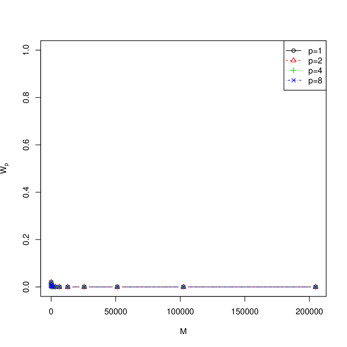
(a) Uniform

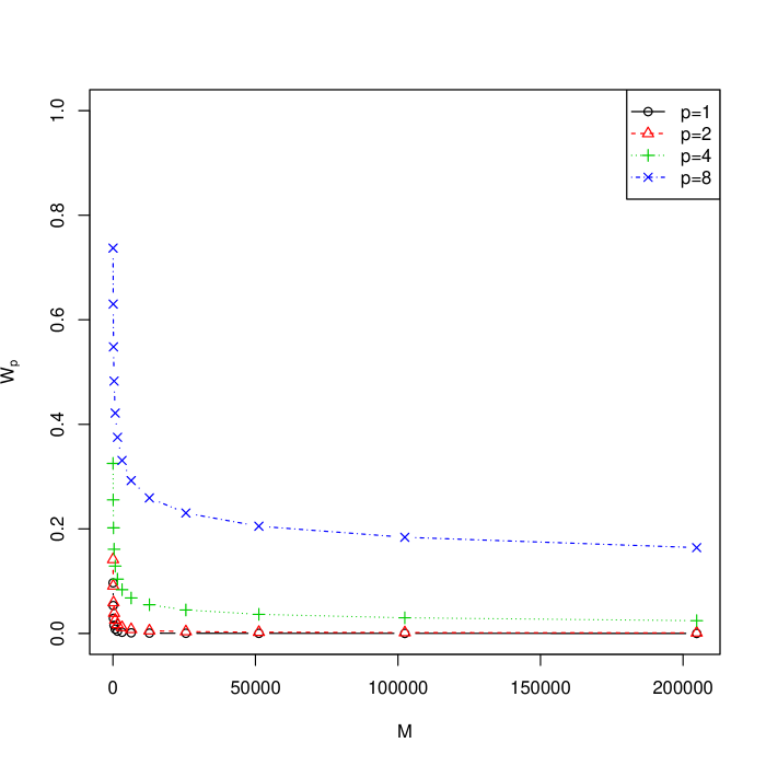
(b) Standard normal

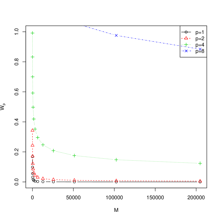
(c) Laplace

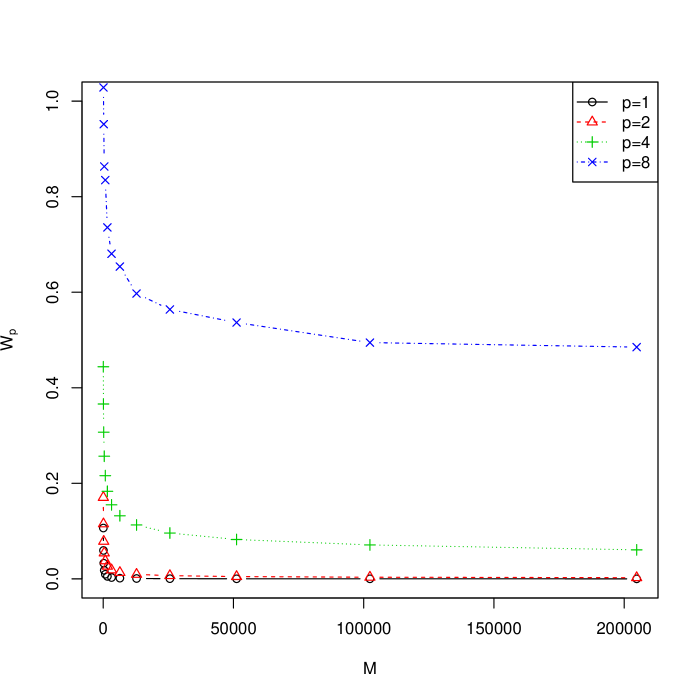
(d) Student’s $t$ with 20 df

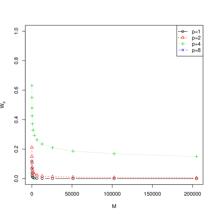
(e) Student’s $t$ with 10 df

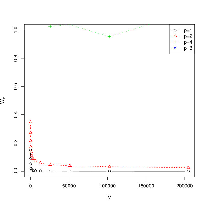
(f) Student’s $t$ with 5 df

Figure 1: The upper bound of $W_{p}(P_{0},{\mathbb{Q}}_{M})$ for various true distributions.

With the above six true distributions, we generated $n=50,100,200,\ldots,6400$ samples and obtained $N=10^{4}$ MCMC samples from the posterior predictive distributions after $1000$ burn-in periods. Then, we evaluated the Wasserstein distance $W_{p}(\widetilde{\mathbb{P}}_{N},{\mathbb{Q}}_{M})$ between the empirical distribution $\widetilde{\mathbb{P}}_{N}$ of MCMC sample and the discrete approximation ${\mathbb{Q}}_{M}$ of $P_{0}$ with $M=2\times 10^{5}$. We considered $p=1$ and $p=2$ only because because the approximation by ${\mathbb{Q}}_{M}$ is not reliable for large $p$. We repeated the above procedure for 100 times and the median among 100 repetitions are depicted in Figures 2 and 3. As can be seen, the posterior predictive distributions become closer to the approximation ${\mathbb{Q}}_{M}$ of the true distribution as the sample size increases. Interestingly, it seems that the location-scale mixture prior also gives consistent posterior distributions with respect to both $W_{1}$ and $W_{2}$ for all cases. Figure 4 shows similar results with a location mixture prior with different hyperparameter $H=N(0,10^{4})$. Note that a normal distribution with large variance is a natural choice for $H$ in practice. The results in Figure 4 shows that the posterior distribution seems to be consistent with respect to $W_{2}$, but more samples are needed to dominate prior probabilities on the tail. This is because some posterior predictive samples might be very large when the number of observation is small, and $W_{2}(\widetilde{\mathbb{P}}_{N},{\mathbb{Q}}_{M})$ is more sensitive to these large samples than $W_{1}(\widetilde{\mathbb{P}}_{N},{\mathbb{Q}}_{M})$.

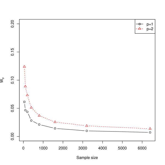
(a) $P_{0}=$Uniform, location

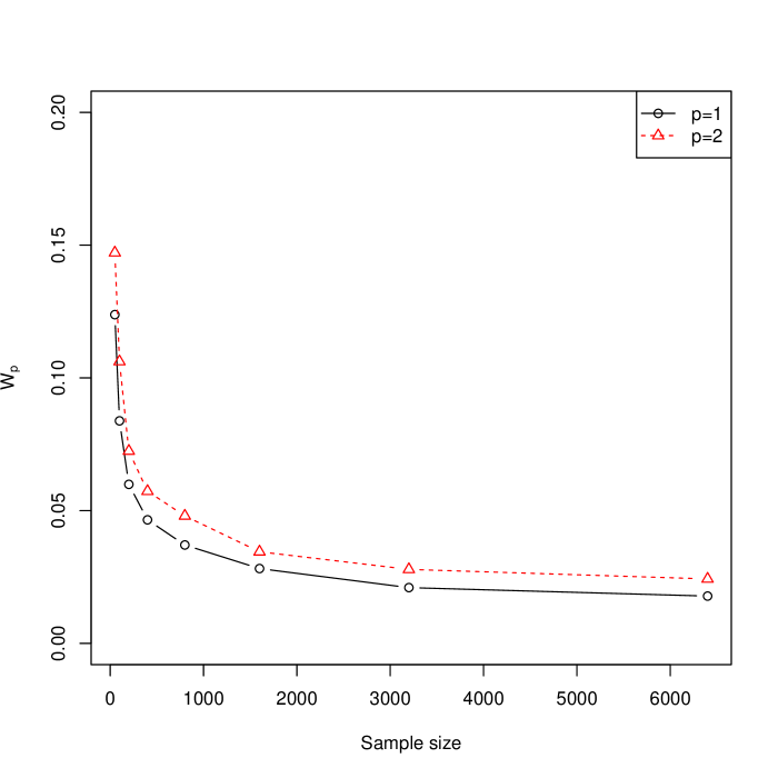
(b) $P_{0}=$Normal, location

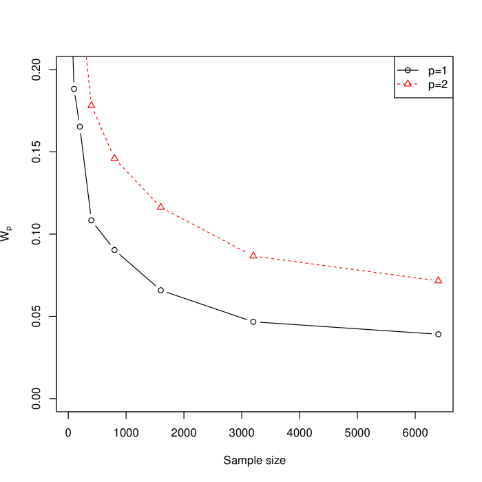
(c) $P_{0}=$Laplace, location

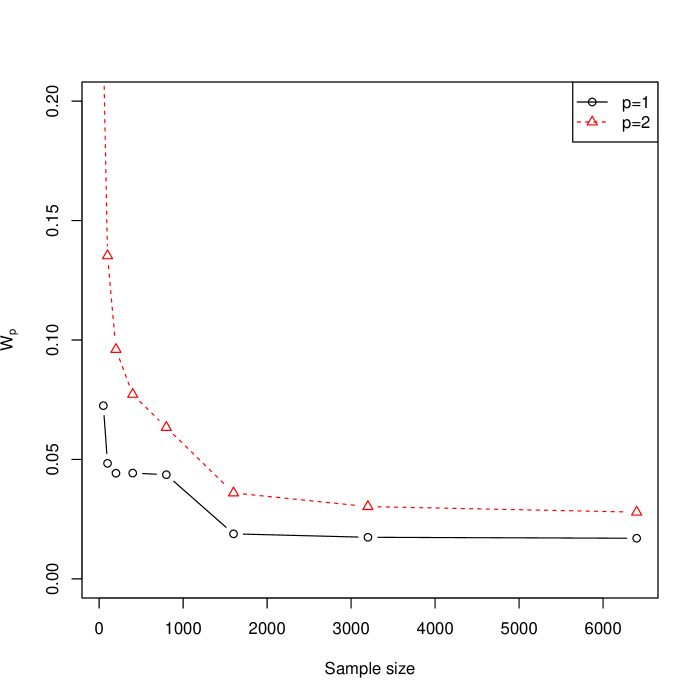
(d) Location-scale mixture

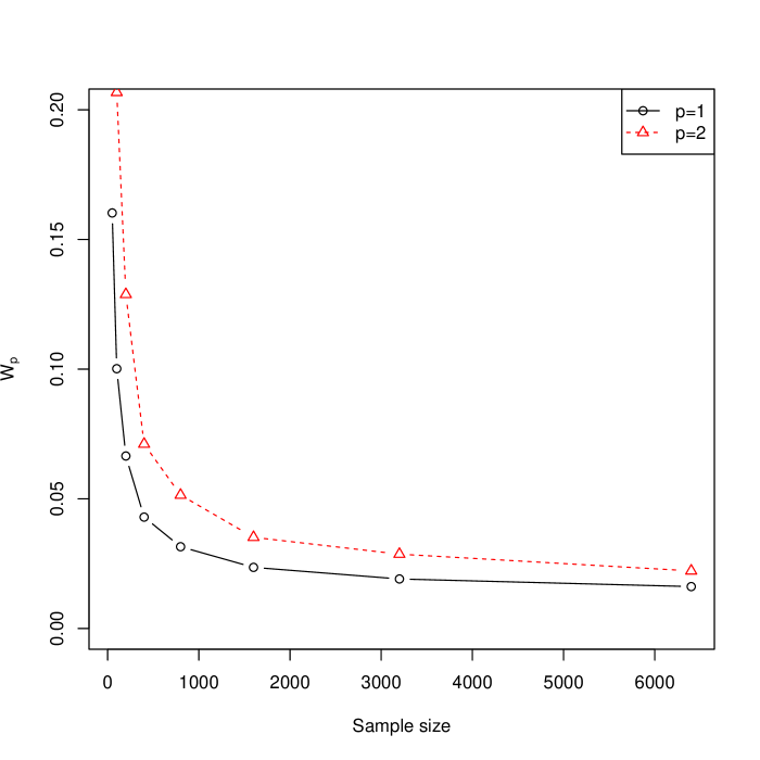
(e) Location-scale mixture

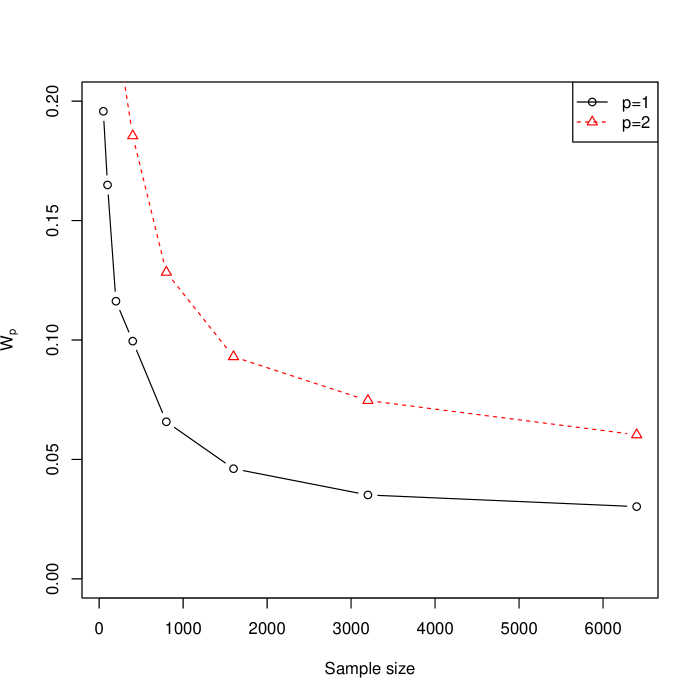
(f) Location-scale mixture

Figure 2: Wasserstein distances between the true distribution–uniform (left), normal (middle), and Laplace (right)–and the posterior predictive distributions based on location (upper) and location-scale mixtures (lower) of Gaussians.

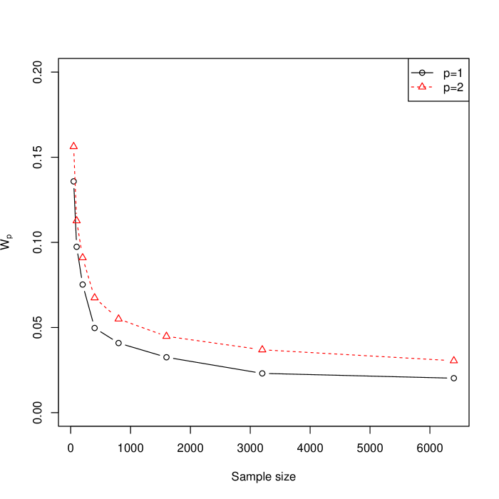
(a) $P_{0}=t$ with 20 df, location

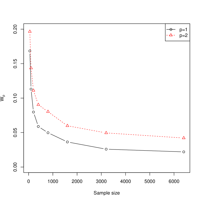
(b) $P_{0}=t$ with 10 df, location

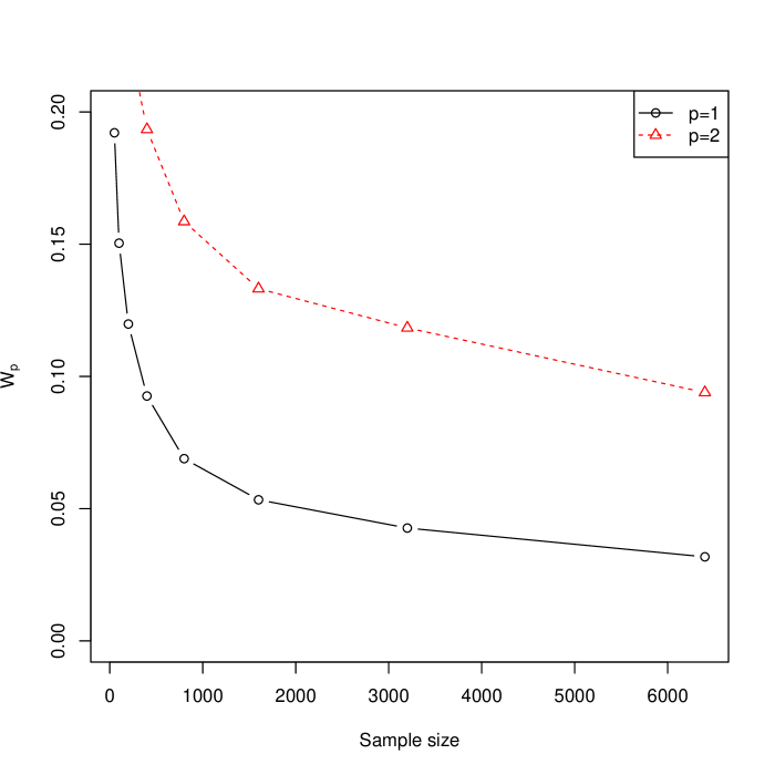
(c) $P_{0}=t$ with 5 df, location

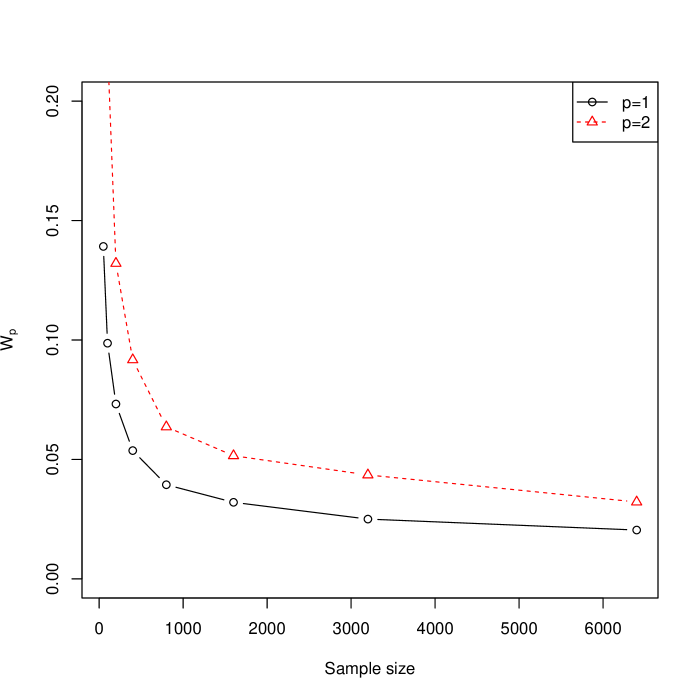
(d) Location-scale mixture

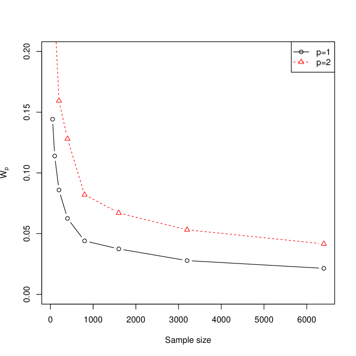
(e) Location-scale mixture

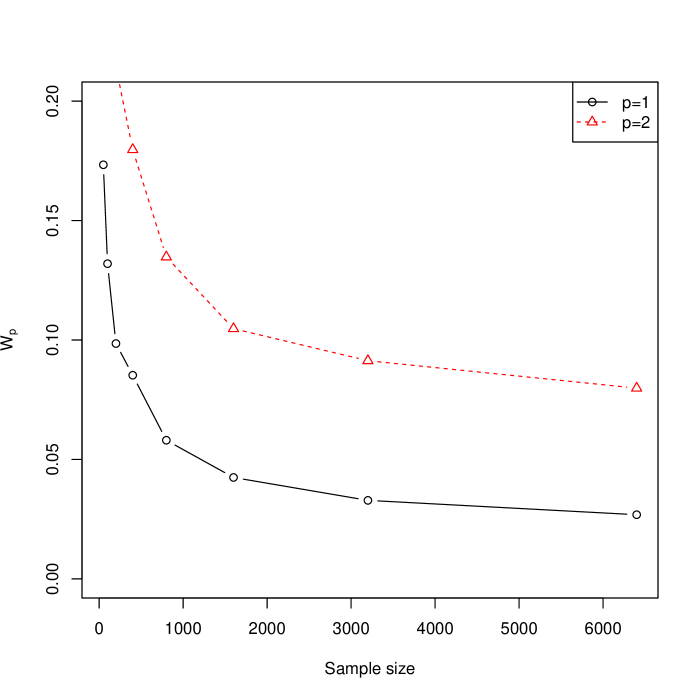
(f) Location-scale mixture

Figure 3: Wasserstein distances between the true distribution–Student’s $t$ distribution with 20 (left), 10 (middle), and 5 (right) degrees of freedom–and the posterior predictive distributions based on location (upper) and location-scale mixtures (lower) of Gaussians.

(a) $P_{0}=$ Uniform

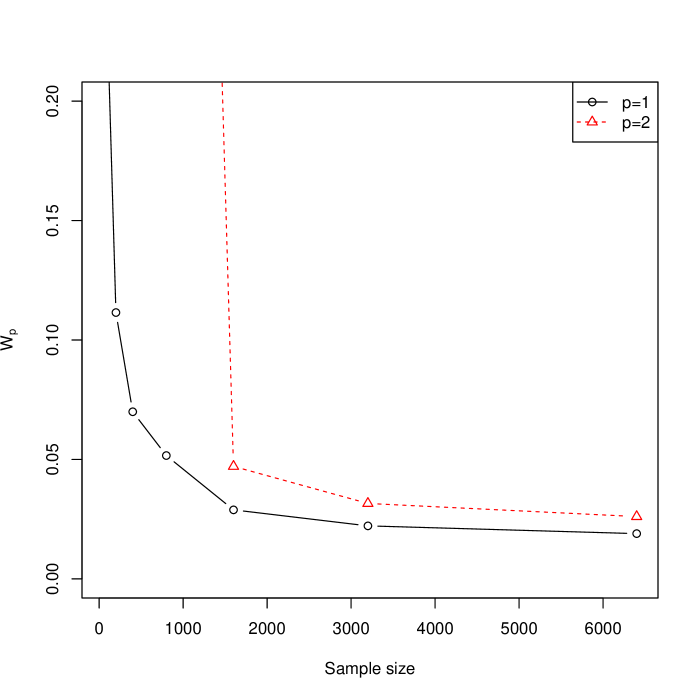
(b) $P_{0}=$ Normal

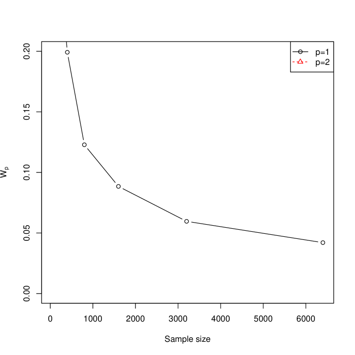
(c) $P_{0}$ Laplace

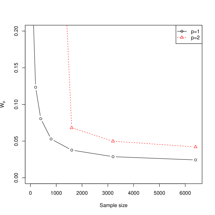
(d) $P_{0}=t$ with 20 df

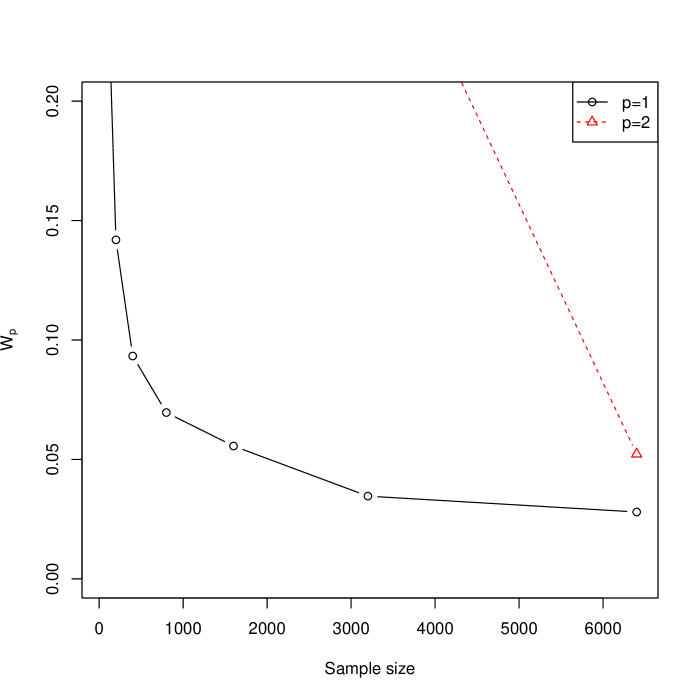
(e) $P_{0}=t$ with 10 df

(f) $P_{0}=t$ with 5 df

Figure 4: Wasserstein distances between the true distributions and the posterior predictive distributions based on the location mixture with $H=N(0,10^{4})$.

7 Discussion

In this paper, we provided sufficient conditions for posterior consistency with respect to the Wasserstein metrics and the convergence rate to be $\epsilon_{n}$ in addition to the well-known KL conditions. Based on our main theorem, the posterior probability that $W_{p}^{p}(P,P_{0})\gtrsim\epsilon_{n}$ vanishes if $M_{2p+\delta}(P)$ is bounded by a constant for some $\delta>0$ with high posterior probability. A similar moment condition has been used in [18] to show that $W_{p}^{p}({\mathbb{P}}_{n},P_{0})\asymp n^{-1/2}$ with high probability. The moment condition cannot be weakened in general as illustrated in our examples. Under a stronger condition (3.3), which is a necessary and sufficient condition for $W_{p}({\mathbb{P}}_{n},P_{0})\asymp n^{-1/2}$, we conjecture that the posterior probability that $W_{p}(P,P_{0})\gtrsim\epsilon_{n}$ would vanish.

We note that asymptotic results given in this paper might be utilized to obtain posterior consistency and its convergence rate with respect to strong metrics such as the total variation. For this, the key is to obtain posterior convergence rate in the Wasserstein metric and bound the total variation between smooth densities by a power of the Wasserstein metric. More precisely, if $P$ and $Q$ possess smooth Lebesgue densities $p$ and $q$, one can prove that $\|p-q\|_{1}\lesssim W_{p}^{\alpha}(P,Q)$ for some $\alpha>0$, see [13] for a sharp inequality. This is a certain reverse inequality because the total variation generates a stronger topology than $W_{p}$ in the space of all probability measures on a bounded metric space. This kind of reverse inequality and related theory for posterior consistency are the main motivation of the present paper, which was firstly considered in [11].

We conclude by discussing an example where total variation consistency and a mild condition implies Wasserstein consistency. This is a non–trivial finding. For a given kernel density function $k$ on ${\mathbb{R}}$, consider a location mixture

$$p(x)=\int k(x-z)dG(z),$$ (7.1)

which is often called a convolution. A prior $\Pi$ on $p$ can be induced from a prior on the mixing distribution $G$. With slight abuse of notation, we use the same notation $\Pi$ for the prior of $G$. Suppose that the true distribution is also of the form (7.1), that is $p_{0}(x)=\int k(x-z)dG_{0}(z)$ for some probability measure $G_{0}$. In this case, posterior consistency with respect to the total variation automatically implies the consistency in $W_{2}$. Suppose that $k$ is symmetric about the origin, $\int x^{2}k(x)dx<\infty$, and that $\tilde{k}(t)\neq 0$ for every $t\in{\mathbb{R}}$, where $\tilde{k}$ is the Fourier transform of $f$ defined as $\tilde{k}(t)=\int e^{-itx}k(x)dx$.

Theorem 7.1.

Suppose that the kernel $k$ satisfies the assumption described above. Assume also that $M_{2}(G_{0})<\infty$ and $\Pi(M_{2}(G)<\infty)=1$. Then, $\mathrm{E}\Pi(\|p-p_{0}\|_{1}>\epsilon\mid X_{1},\ldots,X_{n})\to 0$ for every $\epsilon>0$ implies that

$$\mathrm{E}\Pi\Big{(}W_{2}(P,P_{0})>\epsilon\mid X_{1},\ldots,X_{n}\Big{)}\to 0$$

for every $\epsilon>0$.

Note that the condition $\Pi(M_{2}(G)<\infty)=1$ is easily satisfied for well-known priors. For example, if we put a Dirichlet process prior for $G$, the tail of $G$ is much lighter than that of its mean, see [16]. Posterior consistency with respect to the total variation can also be easily established using a standard technique.

8 Proofs

Firstly, we introduce a basic set-up which is taken from [18] with slight modification, see also [15, 46]. For nonnegative integers $l$, let $\mathcal{P}_{l}$ be the natural partition of $(-1,1]$ into $2^{l}$ translations of $(-2^{-l},2^{-l}]$, that is,

$$\mathcal{P}_{l}=\Big{\{}(-1+k2^{1-l},-1+(k+1)2^{1-l}]:k=0,1,\ldots,2^{l}-1\Big{\}}.$$

Let $B_{0}=(-1,1]$ and $B_{m}=(-2^{m},2^{m}]\backslash(-2^{m-1},2^{m-1}]$ for $m\geq 1$. Let $\pi_{m}:{\mathbb{R}}\rightarrow{\mathbb{R}}$ be the function defined as $\pi_{m}(x)=x/2^{m}$, and $\mathcal{R}_{B_{m}}P$ be the probability measure on $(-1,1]$ defined as the $\pi_{m}$-image of $P|_{B_{m}}/P(B_{m})$, that is, for any Borel set $F\subset(-1,1]$,

$$\mathcal{R}_{B_{m}}P(F)=\frac{P(\pi_{m}^{-1}(F)\cap B_{m})}{P(B_{m})}$$

or $\mathcal{R}_{B_{m}}P(F)=0$ according as $P(B_{m})>0$ or $P(B_{m})=0$.

To get some insight of overall proofs, we next address how one can obtain the consistency of the empirical distribution with respect to $W_{p}$. Suppose for a moment that $P_{0}$ is supported on $[-1,1]$. Then, Lemma 8.3 implies that if $|{\mathbb{P}}_{n}(F)-P_{0}(F)|$ is sufficiently small for every $F\in\mathcal{P}_{l}$ and $l\leq L$, where $L$ is a large enough constant, then $W_{p}({\mathbb{P}}_{n},P_{0})$ will also be small. Since there are various tools to bound the deviation $|{\mathbb{P}}_{n}(F)-P_{0}(F)|$, e.g. the inequality by [26], it is not difficult to prove that the empirical distribution converges to $P_{0}$ in probability with respect to $W_{p}$, $1\leq p<\infty$, with the help of Lemma 8.3.

In case that $P_{0}$ has an unbounded support, Lemma 8.5 can be applied for the Wasserstein consistency of ${\mathbb{P}}_{n}$. Indeed, if $|{\mathbb{P}}_{n}(\pi_{m}^{-1}(F))-P_{0}(\pi_{m}^{-1}(F))|$ is sufficiently small for every $F\in\mathcal{P}_{l}$, $l\leq L$ and $m\leq M$, where $L$ and $M$ are large constants, then $W_{p}({\mathbb{P}}_{n},P_{0})$ will be small. Note that $L$ and $M$ can be chosen as large but fixed constants, so the consistency of ${\mathbb{P}}_{n}$ can be similarly proven using a large deviation inequality such as the Hoeffding’s inequality. Here, it plays an important role that $M_{p}({\mathbb{P}}_{n})$ converges to $M_{p}(P_{0})$ by the law of large numbers, because once the $p$th moment of ${\mathbb{P}}_{n}$ and $P_{0}$ is bounded, it is relatively easy to prove the Wasserstein consistency, see the proof of Theorem 2.2 and Lemma 8.6 for details.

8.1 Frequently used results from literature

The KL condition (1.4) gives a suitable lower bound of the integrated likelihood, that is, the denominator in (1.1). Once this condition holds, the posterior probability of a sequence of subsets $\mathcal{F}_{n}$ of $\mathcal{F}$ can be shown to converge to 1 if the prior probability of $\mathcal{F}_{n}^{c}$ or likelihood is sufficiently small. The latter can often be expressed through the existence of a certain sequence of uniformly consistent tests. Lemmas 8.1 and 8.2 are taken from [20] with slight modification for the simplicity. The rate sequence $\epsilon_{n}$ is assumed that $\epsilon_{n}\rightarrow 0$ and $n\epsilon_{n}^{2}\rightarrow\infty$.

Lemma 8.1.

Suppose that $\Pi(\mathcal{K}_{n})\geq e^{-n\epsilon_{n}^{2}}$ and assume that there exists a sequence of tests $\phi_{n}$ such that

$$P_{0}\phi_{n}\rightarrow 0\quad{\rm and}\quad\sup_{P\in\mathcal{F}_{n}^{c}}P(1-\phi_{n})\leq e^{-3n\epsilon_{n}^{2}}$$

for $\mathcal{F}_{n}\subset\mathcal{F}$. Then, $\Pi\Big{(}\mathcal{F}_{n}^{c}\mid X_{1},\ldots,X_{n}\Big{)}\rightarrow 0$ in probability.

Lemma 8.2.

Suppose that $\Pi(\mathcal{K}_{n})\geq e^{-n\epsilon_{n}^{2}}$ and $\Pi(\mathcal{F}_{n}^{c})\leq e^{-3n\epsilon_{n}^{2}}$ for $\mathcal{F}_{n}\subset\mathcal{F}$. Then, $\Pi\Big{(}\mathcal{F}_{n}^{c}\mid X_{1},\ldots,X_{n}\Big{)}\rightarrow 0$ in probability.

The following lemmas are taken from [18] with slight modification, see also [15, 46]. Since the statement of Lemma 8.3 is slightly different from these papers, we provide a detailed proof for the reader’s convenience.

Lemma 8.3.

Assume that two probability measures $P$ and $Q$ are supported on $(-1,1]$. Then,

$$W_{p}^{p}(P,Q)\leq\kappa_{p}\Bigg{(}\sum_{l=1}^{L}2^{-lp}\sum_{F\in\mathcal{P}_{l}}|P(F)-Q(F)|+2^{-Lp}\Bigg{)}$$

for every $L\geq 1$, where $\kappa_{p}$ is a constant depending only on $p\geq 1$.

Proof.

For a Borel partition $\{A_{k}:k\geq 1\}$ of a Borel set $A\subset{\mathbb{R}}$ and two finite measures $P$ and $Q$ on $A$ with equal mass, define the finite measure $\overline{P}$ as

$$\overline{P}|_{A_{k}}=\frac{Q(A_{k})}{P(A_{k})}P|_{A_{k}}$$

if it is well-defined, that is, $P(A_{k})=0$ implies $Q(A_{k})=0$. Here, $P|_{A_{k}}$ and $\overline{P}|_{A_{k}}$ denote the restrictions of $P$ and $\overline{P}$, respectively, onto $A_{k}$. We say $\overline{P}$ is the $\{A_{k}:k\geq 1\}$-approximation of $P$ to $Q$. Then, we have the following lemma whose proof is explicitly given in [15] (pp. 1189–1190).

Lemma 8.4.

Suppose that the $\{A_{k}:k\geq 1\}$-approximation $\overline{P}$ of $P$ to $Q$ is well-defined. Then, there exists a coupling $\xi$ of $P$ and $\overline{P}$ such that

$$\xi\Big{(}\big{\{}(x,y):x\neq y\big{\}}\Big{)}=\frac{1}{2}\sum_{k\geq 1}|P(A_{k})-Q(A_{k})|.$$

For $l\geq 0$, let $P_{l}$ be the $\mathcal{P}_{l}$-approximation of $P$ to $Q$. We only consider the case that $P_{l}$ is well-defined for all $l\geq 0$. The other case can be handled with further details, see Proposition 1 of [46].

Since $P_{l}(F)=Q(F)$ for $F\in\mathcal{P}_{l}$, we have $W_{p}(P_{l},Q)\leq 2^{-(l-1)}$ for every $l\geq 0$. Furthermore, it is easy to check that, for $F\in\mathcal{P}_{l}$, $P_{l}(F)=P_{l+1}(F)$ and $P_{l+1}|_{F}$ is the $\{C\in\mathcal{P}_{l+1}:C\subset F\}$-approximation of $P_{l}|_{F}$ to $Q|_{F}$. Therefore, by Lemma 8.4, there exists a coupling $\xi_{l+1}$ of $P_{l}$ and $P_{l+1}$ such that

$$\xi_{l+1}\Big{(}\{(x,y):x\neq y\}\Big{)}=\frac{1}{2}\sum_{F\in\mathcal{P}_{l}}\sum_{\begin{subarray}{c}C:C\subset F\\ C\in\mathcal{P}_{l+1}\end{subarray}}\Big{|}P_{l}|_{F}(C)-Q|_{F}(C)\Big{|}$$

$$=\frac{1}{2}\sum_{F\in\mathcal{P}_{l}}\sum_{\begin{subarray}{c}C:C\subset F\\ C\in\mathcal{P}_{l+1}\end{subarray}}\Big{|}P_{l}(C)-Q(C)\Big{|}=\frac{1}{2}\sum_{F\in\mathcal{P}_{l}}\sum_{\begin{subarray}{c}C:C\subset F\\ C\in\mathcal{P}_{l+1}\end{subarray}}\bigg{|}Q(C)-\frac{Q(F)}{P(F)}P(C)\bigg{|}.$$

It follows that there exist random variables $Z_{0},Z_{1},Z_{2},\ldots$ in a same probability space, say $(S,\mathcal{S},\mu)$, such that

$$\mu\Big{(}|Z_{l+1}-Z_{l}|\leq 2^{-(l-1)}\Big{)}=1,$$

$$\mu\Big{(}Z_{l+1}\neq Z_{l}\Big{)}=\frac{1}{2}\sum_{F\in\mathcal{P}_{l}}\sum_{\begin{subarray}{c}C:C\subset F\\ C\in\mathcal{P}_{l+1}\end{subarray}}\left|Q(C)-\frac{Q(F)}{P(F)}P(C)\right|$$

and $Z_{l}$ is marginally distributed as $P_{l}$. Let $N=\inf\{l:Z_{l+1}\neq Z_{l}\}$, where the infimum of the empty set is set to be infinity. Then, conditional on the event $\{N=l\}$ with $l<L$, where $L$ is a fixed positive integer, we have

$$|Z_{0}-Z_{L}|\leq\sum_{l^{\prime}=l}^{L-1}|Z_{l^{\prime}}-Z_{l^{\prime}+1}|\leq 2^{-(l-2)}$$

with probability one. It follows that

$${\mathbb{E}}|Z_{0}-Z_{L}|^{p} \leq \sum_{l=0}^{L-1}{\mathbb{E}}\Big{[}|Z_{0}-Z_{L}|^{p}~{}\Big{|}~{}N=l\Big{]}\mu\Big{(}N=l\Big{)}$$

$$\leq \sum_{l=0}^{L-1}2^{-(l-2)p}\mu\Big{(}Z_{l+1}\neq Z_{l}\Big{)}$$

$$= \frac{1}{2}\sum_{l=0}^{L-1}2^{-(l-2)p}\sum_{F\in\mathcal{P}_{l}}\sum_{\begin{subarray}{c}C:C\subset F\\ C\in\mathcal{P}_{l+1}\end{subarray}}\left|Q(C)-\frac{Q(F)}{P(F)}P(C)\right|.$$

Therefore,

$$W_{p}^{p}(P,Q) \leq 2^{p-1}\Big{(}W_{p}^{p}(P,P_{L})+W_{p}^{p}(P_{L},Q)\Big{)}$$

$$\leq 2^{p-1}\bigg{(}\frac{1}{2}\sum_{l=0}^{L-1}2^{-(l-2)p}\sum_{F\in\mathcal{P}_{l}}\sum_{\begin{subarray}{c}C:C\subset F\\ C\in\mathcal{P}_{l+1}\end{subarray}}\left|Q(C)-\frac{Q(F)}{P(F)}P(C)\right|+2^{-p(L-1)}\bigg{)}$$

Since

$$\left|Q(C)-\frac{Q(F)}{P(F)}P(C)\right| = \frac{1}{P(F)}\Big{|}Q(C)P(F)-Q(F)P(C)\Big{|}$$

$$\leq \frac{1}{P(F)}\Big{[}P(F)|Q(C)-P(C)|+P(C)|P(F)-Q(F)|\Big{]}$$

$$= \frac{P(C)}{P(F)}|P(F)-Q(F)|+|P(C)-Q(C)|,$$

we have

$$\frac{W_{p}^{p}(P,Q)}{2^{p-1}} \leq \frac{1}{2}\sum_{l=0}^{L-1}2^{-(l-2)p}\sum_{F\in\mathcal{P}_{l}}\sum_{\begin{subarray}{c}C:C\subset F\\ C\in\mathcal{P}_{l+1}\end{subarray}}\left[\frac{P(C)}{P(F)}|P(F)-Q(F)|+|P(C)-Q(C)|\right]+2^{-p(L-1)}$$

$$= \frac{1}{2}\sum_{l=0}^{L-1}2^{-(l-2)p}\left[\sum_{F\in\mathcal{P}_{l}}|P(F)-Q(F)|+\sum_{F\in\mathcal{P}_{l+1}}|P(F)-Q(F)|\right]+2^{-p(L-1)}$$

$$= \frac{1}{2}\sum_{l=1}^{L-1}2^{-(l-2)p}\sum_{F\in\mathcal{P}_{l}}|P(F)-Q(F)|+\frac{1}{2}\sum_{l=1}^{L}2^{-(l-3)p}\sum_{F\in\mathcal{P}_{l}}|P(F)-Q(F)|+2^{-p(L-1)}$$

$$\leq \frac{1+2^{p}}{2}\sum_{l=1}^{L}2^{-(l-2)p}\sum_{F\in\mathcal{P}_{l}}|P(F)-Q(F)|+2^{-p(L-1)},$$

where the second equality holds because $\sum_{F\in\mathcal{P}_{0}}|P(F)-Q(F)|=0$. ∎

Lemma 8.5.

For two probability measures $P$ and $Q$ on ${\mathbb{R}}$,

$$\begin{split}W_{p}^{p}(P,Q)\leq\sum_{m\geq 0}2^{mp}\bigg{[}2^{p-1}|P(B_{m})-Q(B_{m})|+\Big{(}P(B_{m})\wedge Q(B_{m})\Big{)}W_{p}^{p}(\mathcal{R}_{B_{m}}P,\mathcal{R}_{B_{m}}Q)\bigg{]}.\end{split}$$ (8.1)

Proof.

The proof is explicitly given in [18] (pp. 714–715). ∎

8.2 Proof of Theorem 2.1

Since the KL condition (1.3) holds, the posterior distribution is consistent with respect to the Lévy-Prokhorov metric $d_{P}$, see Theorem 6.25 of [22]. Therefore, there exists a real sequence $\epsilon_{1n}\downarrow 0$ such that

$$\Pi\Big{(}d_{P}(P,P_{0})>\epsilon_{1n}\mid X_{1},\ldots,X_{n}\Big{)}\longrightarrow 0\quad\text{in probability.}$$

To see this, let $N_{0}=1$, and for every $m\geq 1$, choose $N_{m}>N_{m-1}$ such that

$$\mathrm{E}\left[\Pi\Big{(}d_{P}(P,P_{0})>\frac{1}{m+1}\mid X_{1},\ldots,X_{n}\Big{)}\right]\leq\frac{1}{m+1}\quad\text{for every $n\geq N_{m}$}.$$

Define $\epsilon_{1n}=(m+1)^{-1}$ if $N_{m}\leq n<N_{m+1}$. Then, $\epsilon_{1n}\rightarrow 0$ and for $N_{m}\leq n<N_{m+1}$, we have

$$\mathrm{E}\left[\Pi\Big{(}d_{P}(P,P_{0})>\epsilon_{1n}\mid X_{1},\ldots,X_{n}\Big{)}\right]\leq\frac{1}{m+1}\longrightarrow 0$$

as $n\rightarrow\infty$.

Now, suppose that (2.1) holds. Then, in a similar way, we can construct a sequence $\epsilon_{2n}\downarrow 0$ such that

$$\Pi\Big{(}|M_{p}(P)-M_{p}(P_{0})|>\epsilon_{2n}\mid X_{1},\ldots,X_{n}\Big{)}\longrightarrow 0\quad\text{in probability.}$$

Let

$$\mathcal{F}_{n}=\Big{\{}P\in\mathcal{F}:d_{P}(P,P_{0})\leq\epsilon_{1n},~{}|M_{p}(P)-M_{p}(P_{0})|\leq\epsilon_{2n}\Big{\}}$$

and $P_{n}\in\mathcal{F}_{n}$ such that

$$W_{p}(P_{n},P_{0})\geq\sup_{P\in\mathcal{F}_{n}}W_{p}(P,P_{0})-\epsilon_{1n}.$$

Note that $(P_{n})$ is a non-random sequence of probability measures such that $d_{P}(P_{n},P_{0})\rightarrow 0$ and $M_{p}(P_{n})\rightarrow M_{p}(P_{0})$. It follows that $W_{p}(P_{n},P_{0})\rightarrow 0$. Since $\Pi(\mathcal{F}_{n}\mid X_{1},\ldots,X_{n})\rightarrow 1$ in probability, we conclude that (2.2) holds.

Conversely, suppose that (2.2) holds. Then, similarly as before, we can construct a sequence $\epsilon_{3n}\downarrow 0$ such that

$$\mathrm{E}\left[\Pi\Big{(}W_{p}(P,P_{0})>\epsilon_{3n}\mid X_{1},\ldots,X_{n}\Big{)}\right]\longrightarrow 0.$$

Let

$$\mathcal{F}_{n}^{\prime}=\Big{\{}P\in\mathcal{F}:W_{p}(P,P_{0})\leq\epsilon_{3n}\Big{\}}.$$

and $P_{n}^{\prime}\in\mathcal{F}_{n}^{\prime}$ such that

$$|M_{p}(P_{n}^{\prime})-M_{p}(P_{0})|\geq\sup_{P\in\mathcal{F}_{n}^{\prime}}|M_{p}(P)-M_{p}(P_{0})|-\epsilon_{3n}.$$

Again, $(P_{n}^{\prime})$ is a non-random sequence with $W_{p}(P_{n}^{\prime},P_{0})\rightarrow 0$, so we have $|M_{p}(P_{n}^{\prime})-M_{p}(P_{0})|\rightarrow 0$. Since $\Pi(\mathcal{F}_{n}^{\prime}\mid X_{1},\ldots,X_{n})\rightarrow 1$ in probability, we conclude that (2.1) holds.

∎

8.3 Proof of Theorem 2.2

We first provide a simple proof relying on a stronger moment condition than the one in the statement of Theorem 2.2. For this, we assume that $M_{2p}(P_{0})\leq K$ and

$$\Pi\Big{(}P:\,M_{2p}(P)\leq K\mid X_{1},\ldots,X_{n}\Big{)}\to 1\quad\text{in probability.}$$

In view of the characterization of posterior consistency in the Wasserstein distance of Theorem 2.1, we will establish that $\Pi\Big{(}\mathcal{C}_{j}\mid X_{1},\ldots,X_{n}\Big{)}\rightarrow 0$ in probability for $j=1,2$, where $\mathcal{C}_{1}$ and $\mathcal{C}_{2}$ are the following two convex sets

$$\mathcal{C}_{1} = \left\{P:\,M_{p}(P)-M_{p}(P_{0})>\epsilon,\quad M_{2p}(P)\leq K\right\}$$

$$\mathcal{C}_{2} = \left\{P:\,M_{p}(P_{0})-M_{p}(P)>\epsilon,\quad M_{2p}(P)\leq K\right\}$$

To this aim, it suffices to show that $\inf_{P\in\mathcal{C}_{1}}H(P_{0},P)>0$ and $\inf_{P\in\mathcal{C}_{2}}H(P_{0},P)>0$. For $P\in\mathcal{C}_{1}\cup\mathcal{C}_{2}$, we have

$$|M_{p}(P)-M_{p}(P_{0})|^{2} = \left|\int|x|^{p}\,\Big{(}\sqrt{p(x)/p_{0}(x)}+1\Big{)}\,\Big{(}1-\sqrt{p(x)/p_{0}(x)}\Big{)}\,p_{0}(x)dx\right|^{2}$$

$$\leq H^{2}(P_{0},P)\,\,\int|x|^{2p}\,\Big{(}1+\sqrt{p(x)/p_{0}(x)}\Big{)}^{2}\,p_{0}(x)dx$$

by the Cauchy–Schwarz inequality. The integral of the right term is itself upper bounded by

$$K+2\int|x|^{2p}\,\sqrt{p(x)\,p_{0}(x)}dx+K\leq 4K$$

by virtue of $\sqrt{p\,p_{0}}\leq\hbox{$1\over 2$}(p+p_{0})$. Hence, we get $H(P_{0},P)\geq\epsilon/(2\sqrt{K})$ for $P\in\mathcal{C}_{1}\cup\mathcal{C}_{2}$. ∎

Now, we will prove Theorem 2.2 without the moment condition of order $2p$.

Lemma 8.6.

For positive constants $\epsilon,\delta$ and $K$ assume that

$$P(B_{m})+Q(B_{m})\leq K2^{-(p+\delta)m}\quad\text{for $m\geq 0$},$$ (8.2)

and

$$\Big{|}P(\pi_{m}^{-1}(F)\cap B_{m})-Q(\pi_{m}^{-1}(F)\cap B_{m})\Big{|}\leq\epsilon\quad\text{for $m\leq M,F\in\mathcal{P}_{l},l\leq L$,}$$ (8.3)

where $M$ and $L$ are positive integers. Then,

$$W_{p}^{p}(P,Q)\leq K^{\prime}\left[2^{-\delta M}+2^{-Lp}+2^{Mp}L\epsilon\right],$$

where $K^{\prime}$ is a constant depending only on $\delta,K$ and $p$.

Proof.

Since $W_{p}^{p}(\mathcal{R}_{B_{m}}P,\mathcal{R}_{B_{m}}Q)\leq 2^{p}$ and (8.2) holds, the summation in the right hand side of (8.1) over $m>M$ is bounded by $c_{1}2^{-\delta M}$, where $c_{1}$ is a constant depending only on $\delta,K$ and $p$. Therefore, $W_{p}^{p}(P,Q)$ is bounded by

$$\sum_{m=0}^{M}2^{mp}\bigg{[}2^{p-1}|P(B_{m})-Q(B_{m})|+\Big{(}P(B_{m})\wedge Q(B_{m})\Big{)}W_{p}^{p}(\mathcal{R}_{B_{m}}P,\mathcal{R}_{B_{m}}Q)\bigg{]}+c_{1}2^{-\delta M}$$

by Lemma 8.5. Note that

$$\Big{|}\mathcal{R}_{B_{m}}P(F)-\mathcal{R}_{B_{m}}Q(F)\Big{|}=\left|\frac{P(\pi_{m}^{-1}(F)\cap B_{m})}{P(B_{m})}-\frac{Q(\pi_{m}^{-1}(F)\cap B_{m})}{Q(B_{m})}\right|$$

$$=\frac{|P(\pi_{m}^{-1}(F)\cap B_{m})Q(B_{m})-P(B_{m})Q(\pi_{m}^{-1}(F)\cap B_{m})|}{P(B_{m})Q(B_{m})}$$

$$\leq\frac{1}{P(B_{m})Q(B_{m})}\bigg{[}P(\pi_{m}^{-1}(F)\cap B_{m})\Big{|}P(B_{m})-Q(B_{m})\Big{|}$$

$$\qquad\qquad\qquad\qquad+P(B_{m})\Big{|}P(\pi_{m}^{-1}(F)\cap B_{m})-Q(\pi_{m}^{-1}(F)\cap B_{m})\Big{|}\bigg{]}.$$

By Lemma 8.3 and the last display, we have

$$\begin{split}&\Big{(}P(B_{m})\wedge Q(B_{m})\Big{)}W_{p}^{p}(\mathcal{R}_{B_{m}}P,\mathcal{R}_{B_{m}}Q)\\ &\leq\kappa_{p}\Big{(}P(B_{m})\wedge Q(B_{m})\Big{)}\left[\sum_{l=1}^{L}2^{-lp}\sum_{F\in\mathcal{P}_{l}}|\mathcal{R}_{B_{m}}P(F)-\mathcal{R}_{B_{m}}Q(F)|+2^{-Lp}\right]\\ &\leq\kappa_{p}\bigg{[}\sum_{l=1}^{L}2^{-lp}\left\{\Big{|}P(B_{m})-Q(B_{m})\Big{|}+\sum_{F\in\mathcal{P}_{l}}\Big{|}P(\pi_{m}^{-1}(F)\cap B_{m})-Q(\pi_{m}^{-1}(F)\cap B_{m})\Big{|}\right\}\\ &\qquad+2^{-Lp}\Big{(}P(B_{m})\wedge Q(B_{m})\Big{)}\bigg{]}\\ &\leq\kappa_{p}\bigg{[}\Big{|}P(B_{m})-Q(B_{m})\Big{|}+2^{-Lp}\Big{(}P(B_{m})\wedge Q(B_{m})\Big{)}\\ &\qquad+\sum_{l=1}^{L}2^{-lp}\sum_{F\in\mathcal{P}_{l}}\Big{|}P(\pi_{m}^{-1}(F)\cap B_{m})-Q(\pi_{m}^{-1}(F)\cap B_{m})\Big{|}\bigg{]}.\end{split}$$ (8.4)

It follows that

$$W_{p}^{p}(P,Q) \leq c_{1}2^{-\delta M}+\sum_{m=0}^{M}2^{mp}\bigg{\{}(2^{p-1}+\kappa_{p})\Big{|}P(B_{m})-Q(B_{m})\Big{|}+\kappa_{p}2^{-Lp}\Big{(}P(B_{m})\wedge Q(B_{m})\Big{)}\bigg{\}}$$

$$+\kappa_{p}\sum_{m=0}^{M}2^{mp}\sum_{l=1}^{L}2^{-lp}\sum_{F\in\mathcal{P}_{l}}\Big{|}P(\pi_{m}^{-1}(F)\cap B_{m})-Q(\pi_{m}^{-1}(F)\cap B_{m})\Big{|}$$

$$\leq c_{1}2^{-\delta M}+\epsilon(2^{p-1}+\kappa_{p})\sum_{m=0}^{M}2^{mp}+K\kappa_{p}2^{-Lp}\sum_{m=0}^{M}2^{-\delta m}+\kappa_{p}\epsilon\sum_{m=0}^{M}2^{mp}\sum_{l=1}^{L}2^{-(p-1)l}$$

$$\leq c_{2}\Big{(}2^{-\delta M}+2^{Mp}\epsilon+2^{-Lp}+2^{Mp}L\epsilon\Big{)},$$

where the second inequality holds by (8.2), (8.3) and that the cardinality of $\mathcal{P}_{l}$ is $2^{l}$. Here, $c_{2}$ is a constant depending only on $\delta,K$ and $p$. ∎

By (5.4), we have that

$$P_{0}(B_{m})\leq 2^{p+\delta}K2^{-(p+\delta)m}\quad\text{for $m\geq 0$}.$$

and $\Pi(\mathcal{F}_{0}\mid X_{1},\ldots,X_{n})\rightarrow 1$ in probability, where

$$\mathcal{F}_{0}=\Big{\{}P:P(B_{m})\leq 2^{p+\delta}K2^{-(p+\delta)m}~{}\text{for all $m\geq 0$}\Big{\}}.$$

Suppose that a sufficiently small $\epsilon>0$ is given. We will prove that for some function $g:(0,\infty)\rightarrow(0,\infty)$, with $g(\epsilon)\downarrow 0$ as $\epsilon\downarrow 0$,

$$\Pi\bigg{(}W_{p}^{p}(P,P_{0})\geq g(\epsilon)~{}\Big{|}~{}X_{1},\ldots,X_{n}\bigg{)}\longrightarrow 0\quad\text{in probability}.$$ (8.5)

Let $L$ and $M$ be the largest integer less than or equal to $\log_{2}\epsilon^{-1}$ and $(\log_{2}\epsilon^{-1})/(2p)$, respectively. Then,

$$2^{-\delta M}+2^{-Lp}+2^{Mp}L\epsilon\leq 2^{\delta}\epsilon^{\delta/(2p)}+2^{p}\epsilon^{p}+\sqrt{\epsilon}\log_{2}\epsilon^{-1}.$$ (8.6)

Let

$$\mathcal{F}_{m,F,+} = \Big{\{}P:P(\pi_{m}^{-1}(F)\cap B_{m})-P_{0}(\pi_{m}^{-1}(F)\cap B_{m})<\epsilon\Big{\}}$$

$$\mathcal{F}_{m,F,-} = \Big{\{}P:P_{0}(\pi_{m}^{-1}(F)\cap B_{m})-P(\pi_{m}^{-1}(F)\cap B_{m})<\epsilon\Big{\}}.$$

Then, by Lemma 8.6 and (8.6), there exists a constant $c_{1}$, depending only on $\delta,K$ and $p$, such that

$$P\in\mathcal{F}_{0}\quad\text{and}\quad P\in\bigcap_{m\leq M}\bigcap_{l\leq L}\bigcap_{F\in\mathcal{P}_{l}}(\mathcal{F}_{m,F,+}\cap\mathcal{F}_{m,F,-})\equiv\mathcal{F}_{\epsilon}$$

implies that

$$W_{p}^{p}(P,P_{0})\leq c_{1}\Big{(}2^{\delta}\epsilon^{\delta/(2p)}+2^{p}\epsilon^{p}+\sqrt{\epsilon}\log_{2}\epsilon^{-1}\Big{)}\equiv g(\epsilon).$$

Certainly, $g(\epsilon)\downarrow 0$ as $\epsilon\downarrow 0$. Since $\Pi(\mathcal{F}_{0}^{c}\mid X_{1},\ldots,X_{n})\rightarrow 0$ in probability and the KL condition (1.3) holds, by Schwartz’s theorem (see Theorem 6.25 of [22] if $\Pi$ depends on $n$), it is sufficient for (8.5) to construct a sequence $\phi_{n}$ of tests such that

$$P_{0}\phi_{n}+\sup_{P\in\mathcal{F}_{\epsilon}^{c}}P(1-\phi_{n})\leq e^{-cn}$$ (8.7)

for some constant $c>0$ and every large enough $n$.

Let

$$\phi_{m,F,+} = \left\{\begin{array}[]{ll}1&~{}~{}\text{if ${\mathbb{P}}_{n}(\pi_{m}^{-1}(F)\cap B_{m})-P_{0}(\pi_{m}^{-1}(F)\cap B_{m})>\epsilon/2$}\\ 0&~{}~{}\text{otherwise}\end{array}\right.$$

$$\phi_{m,F,-} = \left\{\begin{array}[]{ll}1&~{}~{}\text{if ${\mathbb{P}}_{n}(\pi_{m}^{-1}(F)\cap B_{m})-P_{0}(\pi_{m}^{-1}(F)\cap B_{m})<-\epsilon/2$}\\ 0&~{}~{}\text{otherwise}.\end{array}\right.$$

Then, by the Hoeffding’s inequality,

$$(P_{0}\phi_{m,F,+})\vee(P_{0}\phi_{m,F,-})\leq e^{-n\epsilon^{2}/2}.$$

Also, for $P\in\mathcal{F}^{c}_{m,F,+}$,

$$P(1-\phi_{m,F,+})\leq P\Big{(}{\mathbb{P}}_{n}(\pi_{m}^{-1}(F)\cap B_{m})-P(\pi_{m}^{-1}(F)\cap B_{m})\leq-\epsilon/2\Big{)}\leq e^{-n\epsilon^{2}/2}$$

by the Hoeffding’s inequality. Similarly, for $P\in\mathcal{F}^{c}_{m,F,-}$,

$$P(1-\phi_{m,F,-})\leq e^{-n\epsilon^{2}/2}.$$

Therefore, if we define

$$\phi_{n}=\max_{m\leq M}\max_{l\leq L}\max_{F\in\mathcal{P}_{l}}(\phi_{m,F,+}\vee\phi_{m,F,-}),$$

then,

$$P_{0}\phi_{n}\leq\sum_{m\leq M}\sum_{l\leq L}\sum_{F\in\mathcal{P}_{l}}P_{0}(\phi_{m,F,+}+\phi_{m,F,-})\leq 2^{L+1}(L+1)(M+1)e^{-n\epsilon^{2}/2}.$$

Since $L,M$ and $\epsilon$ does not depend on $n$, $\phi_{n}$ satisfies (8.7) for some $c>0$ and large enough $n$, which completes the proof. ∎

8.4 Proof of Theorem 3.1

For a given sequence $\delta_{n}$, let

$$\mathcal{C}_{n,1} = \{p:M_{p}(P)-M_{p}(P_{0})>\delta_{n},M_{2p}(P)\leq K\}$$

$$\mathcal{C}_{n,2} = \{p:M_{p}(P_{0})-M_{p}(P)>\delta_{n},M_{2p}(P)\leq K\}$$

and $\mathcal{C}_{n}=\mathcal{C}_{n,1}\cup\mathcal{C}_{n,2}$. Then, it can be shown that

$$\inf_{p\in\mathcal{C}_{n}}H^{2}(p,p_{0})\geq\frac{\delta_{n}^{2}}{4K}$$

as in the first proof of Theorem 2.2. For any measurable set $\mathcal{C}$, let $\Pi_{n}^{\mathcal{C}}$ be the posterior distribution restricted and renormalized onto $\mathcal{C}$, that is,

$$\Pi_{n}^{\mathcal{C}}(A)=\frac{1}{L_{n}(\mathcal{C})}\int_{A}\prod_{i=1}^{n}\frac{p}{p_{0}}(X_{i})d\Pi(p)\quad\text{for all measurable $A\subset\mathcal{C}$}$$

and let $\bar{p}_{n}^{\mathcal{C}}(x)=\int_{\mathcal{C}}p(x)d\Pi_{n}^{\mathcal{C}}(p)$, where

$$L_{n}(\mathcal{C})=\int_{\mathcal{C}}\prod_{i=1}^{n}\frac{p}{p_{0}}(X_{i})d\Pi(p).$$

Since

$$\frac{L_{n}(\mathcal{C})}{L_{n-1}(\mathcal{C})}=\frac{\bar{p}_{n-1}^{\mathcal{C}}}{p_{0}}(X_{n}),$$

we have

$$\mathrm{E}\Big{[}L_{n}^{1/2}(\mathcal{C})\mid\mathcal{G}_{n-1}\Big{]}=L_{n-1}^{1/2}(\mathcal{C})\Big{(}1-\hbox{$1\over 2$}H^{2}(p_{0},\bar{p}_{n-1}^{\mathcal{C}})\Big{)},$$

where $\mathcal{G}_{n-1}$ is the $\sigma$-algebra generated by $X_{1},\ldots,X_{n-1}$. Since $\mathcal{C}_{n,j}$ is convex, we have $H^{2}(p_{0},\bar{p}_{n-1}^{\mathcal{C}_{n,j}})\geq\delta_{n}^{2}/(4K)$ for $j=1,2$. Therefore,

$$\mathrm{E}L_{n}^{1/2}(\mathcal{C}_{n,j})\leq\left(1-\frac{\delta_{n}^{2}}{8K}\right)^{n}\leq e^{-c_{1}n\delta_{n}^{2}}$$

for all large enough $n$, where $c_{1}>0$ is a constant depending only on $K$. It follows that $L_{n}(\mathcal{C}_{n,j})$ is upper bounded by $e^{-c_{2}n\delta_{n}^{2}}$ with probability tending to 1 for some constant $c_{2}$. Thus, if we take $\delta_{n}=K^{\prime}\epsilon_{n}$ for large enough $K^{\prime}$, the proof is complete.

8.5 Proof of Theorem 3.2

Lemma 8.7.

For positive constants $\alpha,\delta,\epsilon$ and $K$, suppose that

$$P(B_{m})+Q(B_{m})\leq K2^{-(2p+\delta)m}\quad\text{for $m\geq 0$},$$ (8.10)

and

$$\Big{|}P(\pi_{m}^{-1}(F)\cap B_{m})-Q(\pi_{m}^{-1}(F)\cap B_{m})\Big{|}\leq\frac{K(2+\alpha)^{-mp}\epsilon}{(l+1)^{2}}\quad\text{for $m\leq M$, $F\in\mathcal{P}_{l}$, $l\leq L$.}$$ (8.11)

Then,

$$W_{p}^{p}(P,Q)\leq K^{\prime}\left[2^{-Lp}+\epsilon+2^{-(p+\delta)M}\right],$$

where $K^{\prime}$ is a constant depending only on $\alpha,K$ and $p$. If $p>1$, condition (8.11) can be replaced by a slightly weaker condition that

$$\Big{|}P(\pi_{m}^{-1}(F)\cap B_{m})-Q(\pi_{m}^{-1}(F)\cap B_{m})\Big{|}\leq K(2+\alpha)^{-mp}\epsilon\quad\text{for $m\leq M$, $F\in\mathcal{P}_{l}$, $l\leq L$.}$$ (8.12)

Proof.

By (8.10) and that $W_{p}^{p}(\mathcal{R}_{B_{m}}P,\mathcal{R}_{B_{m}}Q)\leq 2^{p}$, the summation in the right hand side of (8.1) over $m>M$ is bounded by a constant multiple of $2^{-(p+\delta)M}$. Since $B_{0}\in\mathcal{P}_{0}$,

$$\sum_{m=0}^{M}2^{mp}\big{|}P(B_{m})-Q(B_{m})\big{|} = \sum_{m=0}^{M}2^{mp}\big{|}P(\pi_{m}^{-1}(B_{0})\cap B_{m})-Q(P(\pi_{m}^{-1}(B_{0})\cap B_{m})\big{|}$$

$$\leq K\epsilon\sum_{m=0}^{M}\Big{(}\frac{2}{2+\alpha}\Big{)}^{mp}=K\epsilon\frac{1-(1+\alpha/2)^{-(M+1)p}}{1-(1+\alpha/2)^{-p}},$$

where the inequality holds by (8.11) with $l=0$. Therefore,

$$W_{p}^{p}(P,Q) \leq \sum_{m=0}^{M}2^{mp}\Big{(}P(B_{m})\wedge Q(B_{m})\Big{)}W_{p}^{p}(\mathcal{R}_{B_{m}}P,\mathcal{R}_{B_{m}}Q)+K^{\prime}\Big{(}\epsilon+2^{-(p+\delta)M}\Big{)}$$

by Lemma 8.5, where $K^{\prime}$ is a constant depending only on $\alpha,K$ and $p$. By (LABEL:eq:decompose), the summation in the last display is bounded by

$$\begin{split}\kappa_{p}\sum_{m=0}^{M}2^{mp}&\bigg{[}\Big{|}P(B_{m})-Q(B_{m})\Big{|}+2^{-Lp}\Big{(}P(B_{m})\wedge Q(B_{m})\Big{)}\\ &+\sum_{l=1}^{L}2^{-lp}\sum_{F\in\mathcal{P}_{l}}\Big{|}P(\pi_{m}^{-1}(F)\cap B_{m})-Q(\pi_{m}^{-1}(F)\cap B_{m})\Big{|}\bigg{]}\end{split}$$ (8.13)

Since the cardinality of $\mathcal{P}_{l}$ is $2^{l}$ and $\sum_{l=1}^{\infty}(l+1)^{-2}<\infty$, the first assertion follows from (8.10) and (8.11).

If $p>1$ and (8.11) is replaced by (8.12), we have

$$\sum_{l=1}^{L}2^{-lp}\sum_{F\in\mathcal{P}_{l}}\Big{|}P(\pi_{m}^{-1}(F)\cap B_{m})-Q(\pi_{m}^{-1}(F)\cap B_{m})\Big{|}$$

$$\leq\sum_{l=1}^{L}K2^{-l(p-1)}(2+\alpha)^{-mp}\epsilon\leq\frac{K}{2^{p-1}-1}(2+\alpha)^{-mp}\epsilon.$$

Therefore, we have the same conclusion with a different constant $K^{\prime}$. ∎

Lemma 8.8.

If $X_{1},\ldots,X_{n}\stackrel{{\scriptstyle\rm iid}}{{\sim}}P$, then

$$P({\mathbb{P}}_{n}(B)\leq P(B)-\epsilon) \leq \exp\left(-\frac{n\epsilon^{2}}{2P(B)}\right)$$

$$P({\mathbb{P}}_{n}(B)\geq P(B)+\epsilon) \leq \exp\left(-\frac{n\epsilon^{2}}{2\{P(B)+\epsilon/3\}}\right)$$

for every $n\geq 1$ and $\epsilon\geq 0$.

Proof.

See Theorem 1 of [28]. ∎

Before proving Theorem 3.2, we state and prove a similar one. Theorem 8.9 below is devised for eliminating the logarithmic term $\log\epsilon_{n}^{-1}$ in Theorem 3.2. Proofs of Theorem 3.2 and 8.9 are quite similar, so we do not provide all details to avoid the repetition. We provide a detailed proof only for Theorem 8.9 because this contains the most technical part caused by the factors $(l+1)^{-2}$ and $(l+1)^{-4}$. These factors appear for handling the last term in (8.13). If $p>1$, we need not consider these factors by the second assertion of Lemma 8.7. For $p=1$, we can avoid the technical factors $(l+1)^{-2}$ and $(l+1)^{-4}$, with an additional logarithmic factor in the rate. If we want to eliminate the term $\log\epsilon_{n}^{-1}$, the statement would become more complicated as Theorem 8.9. For conciseness we decided to include Theorem 3.2 in the main texts rather than Theorem 8.9.

Theorem 8.9.

Assume that the prior $\Pi$ satisfies the KL condition (1.4) for a sequence $\epsilon_{n}$ with $\epsilon_{n}\downarrow 0$ and $\epsilon_{n}\geq\sqrt{(\log n)/n}$. Furthermore, assume that there exist positive constants $K$ and $\delta$ such that

$$P_{0}(\pi_{m}^{-1}(F)\cap B_{m})\leq\frac{K}{(l+1)^{4}}2^{-(2p+\delta)m}\quad\text{for $m\geq 0,F\in\mathcal{P}_{l},l\geq 0$}$$

and $\Pi(\mathcal{F}_{n}^{c}\mid X_{1},\ldots,X_{n})\rightarrow 0$ in probability, where

$$\mathcal{F}_{n}=\bigcap_{m\geq 0}\bigcap_{l\leq L}\bigcap_{F\in\mathcal{P}_{l}}\bigg{\{}P:P(\pi_{m}^{-1}(F)\cap B_{m})\leq\frac{K}{(l+1)^{4}}2^{-(2p+\delta)m}\bigg{\}}$$

and $L$ is the largest integer less than or equal to $(\log_{2}\epsilon_{n}^{-1})/p$. Then, for some constant $K^{\prime}>0$,

$$\Pi\bigg{(}W_{p}^{p}(P,P_{0})\geq K^{\prime}\epsilon_{n}~{}\Big{|}~{}X_{1},\ldots,X_{n}\bigg{)}\longrightarrow 0\quad\text{in probability}.$$ (8.14)

Proof.

Let $M$ be the largest integer less than or equal to $(p+\delta)^{-1}\log_{2}\epsilon_{n}^{-1}$. Let $\alpha>0$ be a sufficiently small constant such that $(1+\alpha/2)^{2p}<2^{\delta}$. For $m\leq M$ and $F\in\mathcal{P}_{l}$ with $l\leq L$, let

$$\mathcal{F}_{m,F,+} = \bigg{\{}P\in\mathcal{F}_{n}:P(\pi_{m}^{-1}(F)\cap B_{m})-P_{0}(\pi_{m}^{-1}(F)\cap B_{m})\leq\frac{2K_{1}}{(l+1)^{2}}(2+\alpha)^{-mp}\epsilon_{n}\bigg{\}}$$

$$\mathcal{F}_{m,F,-} = \bigg{\{}P\in\mathcal{F}_{n}:P_{0}(\pi_{m}^{-1}(F)\cap B_{m})-P(\pi_{m}^{-1}(F)\cap B_{m})\leq\frac{2K_{1}}{(l+1)^{2}}(2+\alpha)^{-mp}\epsilon_{n}\bigg{\}},$$

where $K_{1}>0$ is a large constant described below. Then, by Lemma 8.7,

$$P\in\bigcap_{m\leq M}\bigcap_{l\leq L}\bigcap_{F\in\mathcal{P}_{l}}(\mathcal{F}_{m,F,+}\cap\mathcal{F}_{m,F,-})\equiv\mathcal{F}_{n}^{\prime}$$

implies that $W_{p}^{p}(P,P_{0})\leq K_{2}\epsilon_{n}$ for some constant $K_{2}$. Since $\Pi(\mathcal{K}_{n})\geq e^{-n\epsilon_{n}^{2}}$, by Lemma 8.1, it is sufficient for (8.14) to construct a sequence $\phi_{n}$ of tests such that

$$P_{0}\phi_{n}\rightarrow 0\quad{\rm and}\quad\sup_{P\in(\mathcal{F}^{\prime}_{n})^{c}}P(1-\phi_{n})\leq e^{-3n\epsilon_{n}^{2}}$$ (8.15)

for every large enough $n$.

For $m\leq M$ and $F\in\mathcal{P}_{l}$ with $l\leq L$, let

$$\phi_{m,F,+} = \left\{\begin{array}[]{ll}1&~{}~{}\text{if ${\mathbb{P}}_{n}(\pi_{m}^{-1}(F)\cap B_{m})-P_{0}(\pi_{m}^{-1}(F)\cap B_{m})>\frac{K_{1}}{(l+1)^{2}}(2+\alpha)^{-mp}\epsilon_{n}$}\\ 0&~{}~{}\text{otherwise}\end{array}\right.$$

$$\phi_{m,F,-} = \left\{\begin{array}[]{ll}1&~{}~{}\text{if ${\mathbb{P}}_{n}(\pi_{m}^{-1}(F)\cap B_{m})-P_{0}(\pi_{m}^{-1}(F)\cap B_{m})<-\frac{K_{1}}{(l+1)^{2}}(2+\alpha)^{-mp}\epsilon_{n}$}\\ 0&~{}~{}\text{otherwise}.\end{array}\right.$$

Then, by Lemma 8.8,

$$P_{0}\phi_{m,F,+}\leq\exp\left[\frac{-K_{1}^{2}(l+1)^{-4}(2+\alpha)^{-2mp}n\epsilon_{n}^{2}}{2\{P_{0}(\pi_{m}^{-1}(F)\cap B_{m})+K_{1}(l+1)^{-2}(2+\alpha)^{-mp}\epsilon_{n}/3\}}\right].$$

If $P_{0}(\pi_{m}^{-1}(F)\cap B_{m})>K_{1}(l+1)^{-2}(2+\alpha)^{-mp}\epsilon_{n}/3$, then

$$P_{0}\phi_{m,F,+}\leq\exp\left[-\frac{K_{1}^{2}(l+1)^{-4}(2+\alpha)^{-2mp}n\epsilon_{n}^{2}}{4P_{0}(\pi_{m}^{-1}(F)\cap B_{m})}\right]$$

$$\leq\exp\left[-\frac{K_{1}^{2}(2+\alpha)^{-2mp}n\epsilon_{n}^{2}}{4K2^{-(2p+\delta)m}}\right]=\exp\left[-\frac{K_{1}^{2}\beta^{m}n\epsilon_{n}^{2}}{4K}\right],$$

where $\beta=2^{\delta}(1+\alpha/2)^{-2p}>1$. Otherwise,

$$P_{0}\phi_{m,F,+}\leq\exp\left[-\frac{3}{4}K_{1}(l+1)^{-2}(2+\alpha)^{-mp}n\epsilon_{n}\right]$$

$$\leq\exp\left[-\frac{3}{4}K_{1}n\Big{(}\frac{1}{p}\log_{2}\epsilon_{n}^{-1}+1\Big{)}^{-2}\epsilon_{n}^{1+\frac{p\log_{2}(2+\alpha)}{p+\delta}}\right]\leq e^{-K_{1}n\epsilon_{n}^{2}}$$

for large enough $n$, where the second inequality holds because $m\leq M\leq(p+\delta)^{-1}\log_{2}\epsilon_{n}^{-1}$ and $l\leq L\leq(\log_{2}\epsilon_{n}^{-1})/p$, and the third inequality holds because

$$\frac{p\log_{2}(2+\alpha)}{p+\delta}=\frac{\log_{2}(2+\alpha)^{p}}{\log_{2}2^{p+\delta}}\quad\text{and}\quad\frac{(2+\alpha)^{p}}{2^{p+\delta}}=\frac{(1+\alpha/2)^{p}}{2^{\delta}}<1.$$

Since $\epsilon_{n}\geq\sqrt{(\log n)/n}$, we have

$$\sum_{m\leq M}\sum_{l\leq L}\sum_{F\in\mathcal{P}_{l}}P_{0}\phi_{m,F,+}\leq ML2^{L}\max_{m\leq M}\max_{l\leq L}\max_{F\in\mathcal{P}_{l}}P_{0}\phi_{m,F,+}$$

$$\leq\frac{1}{p(p+\delta)}\Big{(}\log_{2}\epsilon_{n}^{-1}\Big{)}^{2}\bigg{(}\frac{1}{\epsilon_{n}}\bigg{)}^{1/p}\max_{m\leq M}\max_{l\leq L}\max_{F\in\mathcal{P}_{l}}P_{0}\phi_{m,F,+}\longrightarrow 0$$

as $n\rightarrow\infty$ provided that $K_{1}$ is large enough. Also, if $K_{1}$ is sufficiently large, for $P\in\mathcal{F}_{m,F,+}^{c}$ with $F\in\mathcal{P}_{l}$,

$$P(1-\phi_{m,F,+})=P\bigg{(}{\mathbb{P}}_{n}(\pi_{m}^{-1}(F)\cap B_{m})-P(\pi_{m}^{-1}(F)\cap B_{m})\leq-\frac{K_{1}}{(l+1)^{2}}(2+\alpha)^{-mp}\epsilon_{n}\bigg{)}$$

$$\leq\exp\left[-\frac{K_{1}^{2}(l+1)^{-4}(2+\alpha)^{-2mp}n\epsilon_{n}^{2}}{2P(\pi_{m}^{-1}(F)\cap B_{m})}\right]\leq\exp\left[-\frac{K_{1}^{2}\beta^{m}}{2K}n\epsilon_{n}^{2}\right]\leq e^{-3n\epsilon_{n}^{2}}$$

for large enough $n$, where the first inequality holds by Lemma 8.8. A similar inequalities for $P_{0}\phi_{m,F,-}$ and $P(1-\phi_{m,F,-})$ can also be obtained. Therefore, if we define

$$\phi_{n}=\max_{m\leq M}\max_{l\leq L}\max_{F\in\mathcal{P}_{l}}(\phi_{m,F,+}\vee\phi_{m,F,-})$$

and $K_{1}$ is sufficiently large, then $\phi_{n}$ satisfies (8.15) for all large enough $n$. This completes the proof. ∎

Proof of Theorem 3.2 for $p>1$. We first claim that if

$$P_{0}(B_{m})\leq K2^{-(2p+\delta)m}\quad\text{for $m\geq 0$}$$

and $\Pi(\mathcal{F}_{0}^{c}\mid X_{1},\ldots,X_{n})\rightarrow 0$ in probability, where

$$\mathcal{F}_{0}=\bigcap_{m\geq 0}\Big{\{}P:P(B_{m})\leq K2^{-(2p+\delta)m}\Big{\}},$$

then (8.14) holds for some constant $K^{\prime}$. The proof of this claim is the same to that of Theorem 8.9 if we replace $\mathcal{F}_{n}$ by $\mathcal{F}_{0}$ and eliminate the factors $(l+1)^{-2}$ and $(l+1)^{-4}$ in all equations, which is possible due to the second assertion of Lemma 8.7.

Once we adjust the constant $K$, two conditions of the claim is satisfied by (5.4). Hence the proof is complete. ∎

Proof of Theorem 3.2 for $p=1$. If (8.10) and (8.12) hold with $p=1$, then it holds that

$$W_{1}(P,Q)\leq K^{\prime}\left[2^{-L}+L\epsilon+2^{-(1+\delta)M}\right].$$ (8.18)

This can be proved as in Lemma 8.7. The only difference is that the last term in (8.13) is bounded as

$$\kappa_{p}\sum_{m=0}^{M}2^{m}\sum_{l=1}^{L}2^{-l}\sum_{F\in\mathcal{P}_{l}}\Big{|}P(\pi_{m}^{-1}(F)\cap B_{m})-Q(\pi_{m}^{-1}(F)\cap B_{m})\Big{|}$$

$$\leq K\kappa_{p}\epsilon\sum_{m=0}^{M}\sum_{l=1}^{L}\Big{(}\frac{2}{2+\alpha}\Big{)}^{m}\leq K^{\prime}L\epsilon,$$

where $K^{\prime}$ is a constant depending only on $\alpha,K$ and $p$.

As in the proof of Theorem 3.2, we next claim that if

$$P_{0}(B_{m})\leq K2^{-(2+\delta)m}\quad\text{for $m\geq 0$}$$

and $\Pi(\mathcal{F}_{0}^{c}\mid X_{1},\ldots,X_{n})\rightarrow 0$ in probability, where

$$\mathcal{F}_{0}=\bigcap_{m\geq 0}\Big{\{}P:P(B_{m})\leq K2^{-(2+\delta)m}\Big{\}},$$

then

$$\Pi\bigg{(}W_{p}^{p}(P,P_{0})\geq K^{\prime}\epsilon_{n}\log\epsilon_{n}^{-1}~{}\Big{|}~{}X_{1},\ldots,X_{n}\bigg{)}\longrightarrow 0\quad\text{in probability}$$

for some constant $K^{\prime}$. To prove this, define $L,M$ and $\alpha$ as in Theorem 8.9 with $p=1$. Also, for $m\leq M$ and $F\in\mathcal{P}_{l}$ with $l\leq L$, let

$$\mathcal{F}_{m,F,+} = \bigg{\{}P\in\mathcal{F}_{0}:P(\pi_{m}^{-1}(F)\cap B_{m})-P_{0}(\pi_{m}^{-1}(F)\cap B_{m})\leq 2K_{1}(2+\alpha)^{-m}\epsilon_{n}\bigg{\}}$$

$$\mathcal{F}_{m,F,-} = \bigg{\{}P\in\mathcal{F}_{0}:P_{0}(\pi_{m}^{-1}(F)\cap B_{m})-P(\pi_{m}^{-1}(F)\cap B_{m})\leq 2K_{1}(2+\alpha)^{-m}\epsilon_{n}\bigg{\}},$$

where $K_{1}>0$ is a large constant as in the proof of Theorem 8.9. Then, by (8.18),

$$P\in\bigcap_{m\leq M}\bigcap_{l\leq L}\bigcap_{F\in\mathcal{P}_{l}}(\mathcal{F}_{m,F,+}\cap\mathcal{F}_{m,F,-})\equiv\mathcal{F}_{n}^{\prime}$$

implies that $W_{p}^{p}(P,P_{0})\leq K_{2}\epsilon_{n}\log\epsilon_{n}^{-1}$ for some constant $K_{2}$. Once we change the definition of $\phi_{n}$ as

$$\phi_{n}=\max_{m\leq M}\max_{l\leq L}\max_{F\in\mathcal{P}_{l}}(\phi_{m,F,+}\vee\phi_{m,F,-}),$$

where

$$\phi_{m,F,+} = \left\{\begin{array}[]{ll}1&~{}~{}\text{if ${\mathbb{P}}_{n}(\pi_{m}^{-1}(F)\cap B_{m})-P_{0}(\pi_{m}^{-1}(F)\cap B_{m})>K_{1}(2+\alpha)^{-m}\epsilon_{n}$}\\ 0&~{}~{}\text{otherwise}\end{array}\right.$$

$$\phi_{m,F,-} = \left\{\begin{array}[]{ll}1&~{}~{}\text{if ${\mathbb{P}}_{n}(\pi_{m}^{-1}(F)\cap B_{m})-P_{0}(\pi_{m}^{-1}(F)\cap B_{m})<-K_{1}(2+\alpha)^{-m}\epsilon_{n}$}\\ 0&~{}~{}\text{otherwise},\end{array}\right.$$

the remaining proof of the claim is the same to that of Theorem 8.9.

Once we adjust the constant $K$, two conditions of the claim is satisfied by (5.4). Hence the proof is complete. ∎

8.6 Proof of Theorem 4.1

Let $\mathcal{F}_{\epsilon}=\{P\in\mathcal{F}_{0}:W_{\infty}(P,P_{0})\leq\epsilon\}$. We will show that for every small enough $\epsilon\geq K_{1}\sqrt{(\log n)/n}$ and $n\geq n_{0}$, there exists a test $\phi$ such that

$$P_{0}\phi\leq e^{-K_{2}n\epsilon^{2}}\quad\textrm{and}\quad\sup_{P\in\mathcal{F}_{2\epsilon}^{c}}P(1-\phi)\leq e^{-K_{2}n\epsilon^{2}},$$ (8.21)

where $K_{1},K_{2}$ and $n_{0}$ are constants depending only on $c_{0}$. Since $\Pi(\mathcal{K}_{n})\geq e^{-n\epsilon_{n}^{2}}$, (8.21) and Lemma 8.1 guarantees (4.1) for large enough constant $K>0$.

Let $\epsilon>0$ be given. Let $N$ be the smallest integer greater than or equal to $\epsilon^{-1}$. Let $I_{j}=[(j-1)\epsilon,j\epsilon)$ for $j=1,\ldots,N-1$ and $I_{N}=[(N-1)\epsilon,1]$. Let $I_{jk}=\cup_{l=j}^{j+k-1}I_{l}$ for $j=1,\ldots,N$ and $k=1,\ldots,N-j+1$. Let ${\mathscr{I}}$ and ${\mathscr{B}}$ be the collections of every interval $I_{jk}$ and every finite union of $I_{jk}$, respectively. Note that the cardinalities of ${\mathscr{I}}$ and ${\mathscr{B}}$ are $N(N+1)/2$ and $2^{N}-1$, respectively.

We first claim that for $P\in\mathcal{F}_{0}$,

$$P(I_{jk})-P_{0}(I_{jk})\leq\frac{c_{0}\epsilon}{2}\;\;\textrm{for every $j$ and $k$ implies that $W_{\infty}(P_{0},P)\leq 2\epsilon$.}$$ (8.22)

If $B$ is either $[0,1]$ or $[0,(N-1)\epsilon)$, it is obvious that $P(B)\leq P_{0}(B^{\epsilon})$. Also, for $B=I_{jk}$ for some $(j,k)$, with $B\neq[0,1]$ and $B\neq[0,(N-1)\epsilon)$,

$$P(B)\leq P_{0}(B)+\frac{c_{0}\epsilon}{2}<P_{0}(B^{\epsilon}).$$

Thus, $P(B)\leq P_{0}(B^{\epsilon})$ for every $B\in{\mathscr{I}}$. For $B\in{\mathscr{B}}-{\mathscr{I}}$, we have $B=\cup_{l=1}^{L}B_{l}$ for some $L\geq 2$, where $B_{l}\in{\mathscr{I}}$ and $B_{l}$’s are $\epsilon$-separated. Thus,

$$P_{0}(B^{\epsilon})\geq\sum_{l=1}^{L}P_{0}(B_{l})+(L-1)c_{0}\epsilon.$$

It follows by (8.22) that

$$P(B)=\sum_{l=1}^{L}P(B_{l})\leq\sum_{l=1}^{L}P_{0}(B_{l})+\frac{Lc_{0}\epsilon}{2}\leq\sum_{l=1}^{L}P_{0}(B_{l})+(L-1)c_{0}\epsilon\leq P_{0}(B^{\epsilon}).$$

Thus, we have $P(B)\leq P_{0}(B^{\epsilon})$ for every $B\in{\mathscr{B}}$. Next, for any Borel subset $A$ of $[0,1]$, let $J=\{j:A\cap I_{j}\neq\emptyset\}$ and $C=\cup_{j\in J}I_{j}$. Then, we have $C\in{\mathscr{B}}$ and $A\subset C\subset A^{\epsilon}$. Therefore,

$$P(A)\leq P(C)\leq P_{0}(C^{\epsilon})\leq P_{0}(A^{2\epsilon}).$$

This proves (8.22).

By (8.22), Then, $\mathcal{F}_{2\epsilon}\supset\cap_{j,k}\mathcal{F}_{jk}$, where

$$\mathcal{F}_{jk}=\{P:P(I_{jk})-P_{0}(I_{jk})\leq c_{0}\epsilon/2\}.$$

Define test functions $\phi_{jk}$ as $\phi_{jk}=1$ if

$${\mathbb{P}}_{n}(I_{jk})>P_{0}(I_{jk})+\frac{c_{0}\epsilon}{4}$$

and $\phi_{jk}=0$ otherwise. Then, for every $P\in\mathcal{F}_{jk}^{c}$, we have

$$P(1-\phi_{jk})=P\left\{{\mathbb{P}}_{n}(I_{jk})\leq P_{0}(I_{jk})+\frac{c_{0}\epsilon}{4}\right\}$$

$$=P\left\{{\mathbb{P}}_{n}(I_{jk})\leq P(I_{jk})+P_{0}(I_{jk})-P(I_{jk})+\frac{c_{0}\epsilon}{4}\right\}$$

$$\leq P\left\{{\mathbb{P}}_{n}(I_{jk})<P(I_{jk})-\frac{c_{0}\epsilon}{4}\right\}\leq\exp\left[-\frac{nc_{0}^{2}\epsilon^{2}}{8}\right],$$

where the last inequality holds by the Hoeffding’s inequality. Let $\phi=\max_{j,k}\phi_{jk}$. Applying the Hoeffding’s inequality again, we have

$$P_{0}\phi\leq\sum_{j,k}P_{0}\phi_{jk}\leq\frac{N(N+1)}{2}\exp\left[-\frac{nc_{0}^{2}\epsilon^{2}}{8}\right]\leq\exp\left[2\log(\epsilon^{-1}+1)-\frac{nc_{0}^{2}\epsilon^{2}}{8}\right].$$ (8.23)

Therefore, we can choose constants $K_{1},K_{2}>0$ and $n_{0}$ such that if $\epsilon\geq K_{1}\sqrt{(\log n)/n}$, then the right hand side of (8.23) is bounded by $\exp(-K_{2}n\epsilon^{2})$ for every $n\geq n_{0}$. This completes the proof of (8.21). ∎

8.7 Proof of Theorem 5.1

Lemma 8.10.

There exist universal constants $c_{1},c_{2}>0$ such that

$$\frac{c_{1}}{\epsilon}\leq\Gamma(\epsilon)\leq\frac{c_{2}}{\epsilon}$$

for every $\epsilon\in(0,1]$.

Proof.

Note that

$$\Gamma(\epsilon)=\int_{0}^{\infty}x^{\epsilon-1}e^{-x}dx=\int_{0}^{1}x^{\epsilon-1}e^{-x}dx+\int_{1}^{\infty}x^{\epsilon-1}e^{-x}dx.$$

It is easy to show that there exist constants $a_{1}$ and $a_{2}$ such that

$$a_{1}\leq\int_{1}^{\infty}x^{\epsilon-1}e^{-x}dx\leq a_{2}$$

for every $\epsilon\in(0,1]$. The assertion follows because $e^{-1}\leq e^{-x}\leq 1$ for every $x\in(0,1]$ and $\int_{0}^{1}x^{\epsilon-1}dx=\epsilon^{-1}$. ∎

Lemma 8.11.

Suppose that $X\sim{\rm Beta}(\alpha\epsilon,\alpha(1-\epsilon))$, $\alpha\epsilon\leq 1$ and $\alpha(1-\epsilon)\geq 1$. Then,

$$P(X>t)\leq C_{\alpha}(1-t^{\alpha\epsilon}),$$

where $C_{\alpha}$ is a constant depending only on $\alpha$.

Proof.

Let $p$ be the pdf of $X$, that is,

$$p(x)=\frac{\Gamma(\alpha)}{\Gamma(\alpha\epsilon)\Gamma(\alpha(1-\epsilon))}x^{\alpha\epsilon-1}(1-x)^{\alpha(1-\epsilon)-1}.$$

By Lemma 8.10,

$$P(X>t)=\int_{t}^{1}p(x)dx\leq c_{\alpha}\epsilon\int_{t}^{1}x^{\alpha\epsilon-1}dx=\frac{c_{\alpha}}{\alpha}(1-t^{\alpha\epsilon}),$$

where $c_{\alpha}$ is a constant depending only on $\alpha$. ∎

Lemma 8.12.

Suppose that $\Pi(\mathcal{K}_{n})\geq e^{-n\epsilon_{n}^{2}}$ and $\epsilon_{n}\geq\sqrt{(\log n)/n}$. Then, there exists a universal constant $K>0$ such that

$$\Pi\Big{(}\big{|}P(B_{m})-P_{0}(B_{m})\big{|}\leq K\epsilon_{n}~{}\forall m\leq C\log\epsilon_{n}^{-1}\mid X_{1},\ldots,X_{n}\Big{)}\rightarrow 1\quad\text{in probability}$$

for every $C>0$.

Proof.

Let $C>0$ be given. For eacn $n$ and $m\leq C\log\epsilon_{n}^{-1}$, let

$$\psi_{m}=I\Big{(}\big{|}{\mathbb{P}}_{n}(B_{m})-P_{0}(B_{m})\big{|}>K\epsilon_{n}/2\Big{)},$$

where $K$ is a universal constant described below. Using the Hoeffding’s inequality, it is not difficult to prove that

$$P_{0}\psi_{m}\lesssim e^{-K^{2}n\epsilon_{n}^{2}/2}\quad{\rm and}\quad\sup_{P\in\mathcal{G}_{m}^{c}}P(1-\psi_{n})\lesssim e^{-K^{2}n\epsilon_{n}^{2}/2},$$

where $\mathcal{G}_{m}=\{P:|P(B_{m})-P_{0}(B_{m})|\leq K\epsilon_{n}\}$. Let

$$\phi_{n}=\max_{m\leq C\log\epsilon_{n}^{-1}}\psi_{m}.$$

Then, we have

$$P_{0}\phi_{n}\lesssim C\log\epsilon_{n}^{-1}e^{-K^{2}n\epsilon_{n}^{2}/2}\rightarrow 0\quad{\rm and}\quad\sup_{P\in\mathcal{F}_{n}^{c}}P(1-\phi_{n})\lesssim e^{-K^{2}n\epsilon_{n}^{2}/2},$$

where

$$\mathcal{F}_{n}=\bigcap_{m\leq C\log\epsilon_{n}^{-1}}\mathcal{G}_{m}.$$

Thus, the proof is complete by Lemma 8.1 provided that $K^{2}/2\geq 3$. ∎

Lemma 8.13.

Let $\epsilon_{n}$ be a sequence such that $\epsilon_{n}\rightarrow 0$ and $\epsilon_{n}\geq\sqrt{\log n/n}$. Let $H$ be the normal distribution with mean $\mu_{H}$ and variance $\sigma^{2}_{H}$. For a Dirichlet process mixture prior (5.2) with $\alpha>1$ and $\sigma=\sigma_{n}\rightarrow 0$, suppose that $\Pi(\mathcal{K}_{n})\geq e^{-n\epsilon_{n}^{2}}$. Also, for some $p\in[1,\infty)$, assume that $P_{0}(B_{m})\leq K2^{-pm}$ for every $m\geq 0$, and that $\epsilon_{n}\leq An^{-p/(2+2p)}$ for every $n$, where $K$ and $A$ are constants. Then,

$$\Pi\Big{(}P(B_{m})\leq K^{\prime}2^{-pm}~{}\forall m\geq 0\mid X_{1},\ldots,X_{n}\Big{)}\rightarrow 1\quad\text{in probability,}$$

where $K^{\prime}$ is a large enough constant.

Proof.

Let $\widetilde{\epsilon}_{n}=L\epsilon_{n}$, and define $\widetilde{\mathcal{K}}_{n}$ as $\mathcal{K}_{n}$ after replacing $\epsilon_{n}$ by $\widetilde{\epsilon}_{n}$, where $L$ is a large constant described below. Then, $\Pi(\widetilde{\mathcal{K}}_{n})\geq\Pi(\mathcal{K}_{n})\geq e^{-n\epsilon_{n}^{2}}$. Note that

$$G(B)\sim{\rm Beta}\Big{(}\alpha H(B),\alpha\big{(}1-H(B)\big{)}\Big{)}$$

for any Borel set $B$. Also, $\alpha H(\overline{B}_{m})\leq 1$ and $\alpha(1-H(\overline{B}_{m}))\geq 1$ for every large enough $m$, where

$$\overline{B}_{m}=(-\infty,-2^{m-1}]\cup(2^{m-1},\infty).$$

Thus, by Lemma 8.11, for any $K^{\prime}\geq 2^{p}$,

$$\begin{split}&\Pi\big{(}G(B_{m})>K^{\prime}2^{-pm}\big{)}\leq\Pi\big{(}G(\overline{B}_{m})>K^{\prime}2^{-pm}\big{)}\\ &\leq\Pi\big{(}G(\overline{B}_{m})>2^{-pm}\big{)}\leq C_{\alpha}\big{(}1-2^{-pm\alpha H(\overline{B}_{m})}\big{)}\end{split}$$ (8.24)

for every large enough $m$, where $C_{\alpha}$ is a constant depending only on $\alpha$. Note that $1-\Phi_{\sigma}(x)\leq e^{-x^{2}/(2\sigma^{2})}/2$, where $\Phi_{\sigma}$ is the cdf of $\phi_{\sigma}$, so we have

$$H(\overline{B}_{m})\leq\frac{1}{2}\left[\exp\left\{-\frac{1}{2}\left(\frac{2^{m-1}-\mu_{H}}{\sigma_{H}}\right)^{2}\right\}+\exp\left\{-\frac{1}{2}\left(\frac{2^{m-1}+\mu_{H}}{\sigma_{H}}\right)^{2}\right\}\right].$$

Since $1-e^{-x}\leq x$, the right hand side of (LABEL:eq:G_B_prob) is bounded by

$$\frac{\log 2}{2}p\alpha C_{\alpha}m\left[\exp\left\{-\frac{1}{2}\left(\frac{2^{m-1}-\mu_{H}}{\sigma_{H}}\right)^{2}\right\}+\exp\left\{-\frac{1}{2}\left(\frac{2^{m-1}+\mu_{H}}{\sigma_{H}}\right)^{2}\right\}\right]$$

$$\lesssim p\alpha C_{\alpha}\exp\{-C_{\sigma_{H}}2^{2m}\}$$

for every large enough $m$, where $C_{\sigma_{H}}$ is a constant depending only on $\sigma_{H}$.

Note that $P$ is the convolution of $G$ and $N(0,\sigma_{n}^{2})$. If $Y_{1}=Y_{2}+Y_{3}$, where $Y_{2}$ and $Y_{3}$ are independent random variables following $G$ and $N(0,\sigma_{n}^{2})$, respectively, then

$$P(\overline{B}_{m})=\Pr(|Y_{1}|>2^{m-1}) \leq \Pr(|Y_{2}|>2^{m-2})+\Pr(|Y_{3}|>2^{m-2})$$

$$\leq G(\overline{B}_{m-1})+2\big{(}1-\Phi_{\sigma_{n}}(2^{m-2})\big{)}.$$

Hence,

$$P(B_{m})\leq P(\overline{B}_{m})\leq G(\overline{B}_{m-1})+2\big{(}1-\Phi_{\sigma_{n}}(2^{m-2})\big{)}$$

$$\leq G(\overline{B}_{m-1})+\exp\left(-\frac{2^{2(m-2)}}{2\sigma_{n}^{2}}\right)\leq G(\overline{B}_{m-1})+2^{-pm},$$

where the last inequality holds for every large enough $m$. It follows for any constants $C>0$ and large enough $n$ that

$$\Pi\big{(}P(B_{m})>(K^{\prime}+1)2^{-pm}~{}\text{for some $m\geq C\log\widetilde{\epsilon}_{n}^{-1}$}\big{)}$$

$$\leq\Pi\big{(}G(\overline{B}_{m-1})>K^{\prime}2^{-pm}~{}\text{for some $m\geq C\log\widetilde{\epsilon}_{n}^{-1}$}\big{)}$$

$$=\Pi\big{(}G(\overline{B}_{m})>K^{\prime}2^{-p(m+1)}~{}\text{for some $m\geq C\log\widetilde{\epsilon}_{n}^{-1}-1$}\big{)}$$

$$\leq\sum_{m\geq C\log\widetilde{\epsilon}_{n}^{-1}-1}\Pi\big{(}G(\overline{B}_{m})>2^{-pm}\big{)}$$

$$\lesssim p\alpha C_{\alpha}\sum_{m\geq C\log\widetilde{\epsilon}_{n}^{-1}-1}\exp\left(-C_{\sigma_{H}}2^{2m}\right)\lesssim p\alpha C_{\alpha}\exp\left(-\frac{C_{\sigma_{H}}}{4}\widetilde{\epsilon}_{n}^{-2C\log 2}\right).$$

If we take $C=(p\log 2)^{-1}$, the right hand side of the last display is bounded by

$$p\alpha C_{\alpha}\exp\left(-\frac{C_{\sigma_{H}}}{4}\widetilde{\epsilon}_{n}^{-2/p}\right).$$

Since $\epsilon_{n}\leq An^{-p/(2+2p)}$, $n\epsilon_{n}^{2}$ is bounded by a constant multiple of $\epsilon_{n}^{-2/p}$ for every $n$. Hence, if $L$ is large enough, we have that

$$\Pi\Big{(}P(B_{m})>(K^{\prime}+1)2^{-pm}~{}\text{for some $m\geq C\log\widetilde{\epsilon}_{n}^{-1}$}\mid X_{1},\ldots,X_{n}\Big{)}\rightarrow 0~{}\text{in probability}$$

by Lemma 8.2.

Note that by Lemma 8.12,

$$\Pi\Big{(}\big{|}P(B_{m})-P_{0}(B_{m})\big{|}\leq K^{\prime\prime}\widetilde{\epsilon}_{n}~{}\forall m\leq C\log\widetilde{\epsilon}_{n}^{-1}\mid X_{1},\ldots,X_{n}\Big{)}\rightarrow 1\quad\text{in probability},$$

where $K^{\prime\prime}$ is a constant. Since

$$P_{0}(B_{m})+K^{\prime\prime}\widetilde{\epsilon}_{n}\leq(K+K^{\prime\prime})2^{-pm}$$

for every $m\leq C\log\widetilde{\epsilon}_{n}^{-1}$, the proof is complete. ∎

It is shown in the proof of Theorem 2 in [21] that $\Pi(\mathcal{K}_{n})\geq e^{-n\epsilon_{n}^{2}}$ with $\epsilon_{n}=cn^{-2/5}(\log n)^{2}$ for some constant $c>0$. For any $p<4$, note that $\epsilon_{n}\leq n^{-p/(2+2p)}$ for all large enough $n$. Hence, the proof of Theorem 5.1 is complete by (5.4) and Lemma 8.13. ∎

8.8 Proof of Theorem 7.1

Denote $p_{G}(x)=\int k_{\sigma}(x-z)dG(z)$. We use the result of [36]. It is shown in the proof of Theorem 2 in [36] that

$$W_{2}^{2}(G,G_{0})$$

$$\leq C\inf_{\delta\in(0,1)}\left[\delta^{2}+\|p_{G}-p_{G_{0}}\|_{1}^{2(s-2)/(1+2s)}\bigg{\{}\int_{-1/\delta}^{1/\delta}\tilde{k}(t)^{-2}dt\bigg{\}}^{(s-2)/(1+2s)}\right]$$

for any $s>2$ and $G$ with $M_{2}(G)<\infty$, where $C$ is a constant depending only on $s$. Note that Theorem 2 of [36] assumed that $G$ and $G_{0}$ are discrete probability measures with bounded supports, but finiteness of the second moment suffices as discussed therein. The right hand side of the last display tends to zero as $\|p_{G}-p_{G_{0}}\|_{1}\to 0$. It follows that for every $\epsilon>0$,

$$\Pi\Big{(}W_{2}^{2}(G,G_{0})>\epsilon\mid X_{1},\ldots,X_{n}\Big{)}\to 0.$$

in probability. Since $W_{2}^{2}(P_{G},P_{G_{0}})\leq W_{2}^{2}(G,G_{0})$, the proof is complete. ∎

References

Arjovsky, Chintala and
Bottou [2017]{binproceedings}[author]
\bauthor\bsnmArjovsky, \bfnmMartin\binitsM.,
\bauthor\bsnmChintala, \bfnmSoumith\binitsS. and \bauthor\bsnmBottou, \bfnmLéon\binitsL.
(\byear2017).
\btitleWasserstein generative adversarial networks.
In \bbooktitleProc. International Conference on Machine Learning
\bpages214–223.
\endbibitem
Barron, Schervish and
Wasserman [1999]{barticle}[author]
\bauthor\bsnmBarron, \bfnmAndrew\binitsA.,
\bauthor\bsnmSchervish, \bfnmMark J\binitsM. J. and \bauthor\bsnmWasserman, \bfnmLarry\binitsL.
(\byear1999).
\btitleThe consistency of posterior distributions in nonparametric problems.
\bjournalAnn. Statist.
\bvolume27
\bpages536–561.
\endbibitem
Bernton et al. [2019]{barticle}[author]
\bauthor\bsnmBernton, \bfnmEspen\binitsE.,
\bauthor\bsnmJacob, \bfnmPierre E.\binitsP. E.,
\bauthor\bsnmGerber, \bfnmMathieu\binitsM. and \bauthor\bsnmRobert, \bfnmChristian P.\binitsC. P.
(\byear2019).
\btitleApproximate Bayesian computation with the Wasserstein distance.
\bjournalJ. R. Stat. Soc. Ser. B. Stat. Methodol.
\bvolume81
\bpages235-269.
\endbibitem
Biau, Devroye and
Lugosi [2008]{barticle}[author]
\bauthor\bsnmBiau, \bfnmGérard\binitsG.,
\bauthor\bsnmDevroye, \bfnmLuc\binitsL. and \bauthor\bsnmLugosi, \bfnmGábor\binitsG.
(\byear2008).
\btitleOn the performance of clustering in Hilbert spaces.
\bjournalIEEE Trans. Inform. Theory
\bvolume54
\bpages781–790.
\endbibitem
Biau et al. [2018]{barticle}[author]
\bauthor\bsnmBiau, \bfnmGérard\binitsG.,
\bauthor\bsnmCadre, \bfnmBenoît\binitsB.,
\bauthor\bsnmSangnier, \bfnmMAXIME\binitsM. and \bauthor\bsnmTanielian, \bfnmUgo\binitsU.
(\byear2018).
\btitleSome theoretical properties of GANs.
\bjournalarXiv:1803.07819.
\endbibitem
Bickel and
Kleijn [2012]{barticle}[author]
\bauthor\bsnmBickel, \bfnmPJ\binitsP. and \bauthor\bsnmKleijn, \bfnmBJK\binitsB.
(\byear2012).
\btitleThe semiparametric Bernstein–von Mises theorem.
\bjournalAnn. Statist.
\bvolume40
\bpages206–237.
\endbibitem
Bobkov and Ledoux [2019]{bbook}[author]
\bauthor\bsnmBobkov, \bfnmSergey\binitsS. and \bauthor\bsnmLedoux, \bfnmMichel\binitsM.
(\byear2019).
\btitleOne-dimensional empirical measures, order statistics, and Kantorovich
transport distances
\bvolume261.
\bpublisherMemoirs of the American Mathematical Society.
\endbibitem
Castillo and
Nickl [2014]{barticle}[author]
\bauthor\bsnmCastillo, \bfnmIsmaël\binitsI. and \bauthor\bsnmNickl, \bfnmRichard\binitsR.
(\byear2014).
\btitleOn the Bernstein–von Mises phenomenon for nonparametric Bayes
procedures.
\bjournalAnn. Statist.
\bvolume42
\bpages1941–1969.
\endbibitem
Castillo and
Rousseau [2015]{barticle}[author]
\bauthor\bsnmCastillo, \bfnmIsmaël\binitsI. and \bauthor\bsnmRousseau, \bfnmJudith\binitsJ.
(\byear2015).
\btitleA Bernstein–von Mises theorem for smooth functionals in
semiparametric models.
\bjournalAnn. Statist.
\bvolume43
\bpages2353–2383.
\endbibitem
Chae, Kim and
Kleijn [2019]{barticle}[author]
\bauthor\bsnmChae, \bfnmMinwoo\binitsM.,
\bauthor\bsnmKim, \bfnmYongdai\binitsY. and \bauthor\bsnmKleijn, \bfnmBas\binitsB.
(\byear2019).
\btitleThe semi-parametric Bernstein–von Mises theorem for regression models
with symmetric errors.
\bjournalStatist. Sinica
\bvolume29.
\endbibitem
Chae and Walker [2017]{barticle}[author]
\bauthor\bsnmChae, \bfnmMinwoo\binitsM. and \bauthor\bsnmWalker, \bfnmStephen G\binitsS. G.
(\byear2017).
\btitleA novel approach to Bayesian consistency.
\bjournalElectron. J. Stat.
\bvolume11
\bpages4723–4745.
\endbibitem
Chae and
Walker [2019]{barticle}[author]
\bauthor\bsnmChae, \bfnmMinwoo\binitsM. and \bauthor\bsnmWalker, \bfnmStephen G\binitsS. G.
(\byear2019).
\btitleBayesian consistency for a nonparametric stationary Markov model.
\bjournalBernoulli
\bvolume25
\bpages877–901.
\endbibitem
Chae and Walker [2020]{barticle}[author]
\bauthor\bsnmChae, \bfnmMinwoo\binitsM. and \bauthor\bsnmWalker, \bfnmStephen G\binitsS. G.
(\byear2020).
\btitleWasserstein upper bounds of the total variation for smooth densities.
\bjournalStatist. Probab. Lett.
\bvolume163
\bpages1–6.
\endbibitem
De Acosta [1982]{barticle}[author]
\bauthor\bsnmDe Acosta, \bfnmAlejandro\binitsA.
(\byear1982).
\btitleInvariance principles in probability for triangular arrays of
-valued random vectors and some applications.
\bjournalAnn. Probab.
\bvolume10
\bpages346–373.
\endbibitem
Dereich, Scheutzow and
Schottstedt [2013]{barticle}[author]
\bauthor\bsnmDereich, \bfnmSteffen\binitsS.,
\bauthor\bsnmScheutzow, \bfnmMichael\binitsM. and \bauthor\bsnmSchottstedt, \bfnmReik\binitsR.
(\byear2013).
\btitleConstructive quantization: Approximation by empirical measures.
\bjournalAnn. Inst. Henri Poincaré Probab. Stat.
\bvolume49
\bpages1183–1203.
\endbibitem
Doss and Sellke [1982]{barticle}[author]
\bauthor\bsnmDoss, \bfnmHani\binitsH. and \bauthor\bsnmSellke, \bfnmThomas\binitsT.
(\byear1982).
\btitleThe tails of probabilities chosen from a Dirichlet prior.
\bjournalAnn. Statist.
\bvolume10
\bpages1302–1305.
\endbibitem
Dudley [1989]{bbook}[author]
\bauthor\bsnmDudley, \bfnmRichard M\binitsR. M.
(\byear1989).
\btitleReal Analysis and Probability.
\bpublisherChapman and Hall/CRC.
\endbibitem
Fournier and Guillin [2015]{barticle}[author]
\bauthor\bsnmFournier, \bfnmNicolas\binitsN. and \bauthor\bsnmGuillin, \bfnmArnaud\binitsA.
(\byear2015).
\btitleOn the rate of convergence in Wasserstein distance of the empirical
measure.
\bjournalProbab. Theory Related Fields
\bvolume162
\bpages707–738.
\endbibitem
Ghosal, Ghosh and
Ramamoorthi [1999]{barticle}[author]
\bauthor\bsnmGhosal, \bfnmSubhashis\binitsS.,
\bauthor\bsnmGhosh, \bfnmJayanta K\binitsJ. K. and \bauthor\bsnmRamamoorthi, \bfnmRV\binitsR.
(\byear1999).
\btitlePosterior consistency of Dirichlet mixtures in density estimation.
\bjournalAnn. Statist.
\bvolume27
\bpages143–158.
\endbibitem
Ghosal, Ghosh and van der
Vaart [2000]{barticle}[author]
\bauthor\bsnmGhosal, \bfnmSubhashis\binitsS.,
\bauthor\bsnmGhosh, \bfnmJayanta K\binitsJ. K. and \bauthor\bparticlevan der \bsnmVaart, \bfnmAad W\binitsA. W.
(\byear2000).
\btitleConvergence rates of posterior distributions.
\bjournalAnn. Statist.
\bvolume28
\bpages500–531.
\endbibitem
Ghosal and van der
Vaart [2007]{barticle}[author]
\bauthor\bsnmGhosal, \bfnmSubhashis\binitsS. and \bauthor\bparticlevan der \bsnmVaart, \bfnmAad W\binitsA. W.
(\byear2007).
\btitlePosterior convergence rates of Dirichlet mixtures at smooth
densities.
\bjournalAnn. Statist.
\bvolume35
\bpages697–723.
\endbibitem
Ghosal and van der
Vaart [2017]{bbook}[author]
\bauthor\bsnmGhosal, \bfnmSubhashis\binitsS. and \bauthor\bparticlevan der \bsnmVaart, \bfnmAad\binitsA.
(\byear2017).
\btitleFundamentals of Nonparametric Bayesian Inference.
\bpublisherCambridge University Press.
\endbibitem
Gibbs and Su [2002]{barticle}[author]
\bauthor\bsnmGibbs, \bfnmAlison L\binitsA. L. and \bauthor\bsnmSu, \bfnmFrancis Edward\binitsF. E.
(\byear2002).
\btitleOn choosing and bounding probability metrics.
\bjournalInt. Stat. Rev.
\bvolume70
\bpages419–435.
\endbibitem
Givens and Shortt [1984]{barticle}[author]
\bauthor\bsnmGivens, \bfnmClark R\binitsC. R. and \bauthor\bsnmShortt, \bfnmRae Michael\binitsR. M.
(\byear1984).
\btitleA class of Wasserstein metrics for probability distributions.
\bjournalThe Michigan Mathematical Journal
\bvolume31
\bpages231–240.
\endbibitem
Gulrajani
et al. [2017]{binproceedings}[author]
\bauthor\bsnmGulrajani, \bfnmIshaan\binitsI.,
\bauthor\bsnmAhmed, \bfnmFaruk\binitsF.,
\bauthor\bsnmArjovsky, \bfnmMartin\binitsM.,
\bauthor\bsnmDumoulin, \bfnmVincent\binitsV. and \bauthor\bsnmCourville, \bfnmAaron C\binitsA. C.
(\byear2017).
\btitleImproved training of Wasserstein GANs.
In \bbooktitleProc. Neural Information Processing Systems
\bpages5767–5777.
\endbibitem
Hoeffding [1963]{barticle}[author]
\bauthor\bsnmHoeffding, \bfnmWassily\binitsW.
(\byear1963).
\btitleProbability inequalities for sums of bounded random variables.
\bjournalJ. Amer. Statist. Assoc.
\bvolume58
\bpages13–30.
\endbibitem
Janson [2016]{barticle}[author]
\bauthor\bsnmJanson, \bfnmSvante\binitsS.
(\byear2016).
\btitleLarge deviation inequalities for sums of indicator variables.
\bjournalarXiv:1609.00533.
\endbibitem
Kalli, Griffin and
Walker [2011]{barticle}[author]
\bauthor\bsnmKalli, \bfnmMaria\binitsM.,
\bauthor\bsnmGriffin, \bfnmJim E\binitsJ. E. and \bauthor\bsnmWalker, \bfnmStephen G\binitsS. G.
(\byear2011).
\btitleSlice sampling mixture models.
\bjournalStat. Comput.
\bvolume21
\bpages93–105.
\endbibitem
Kantorovich and
Rubinstein [1958]{barticle}[author]
\bauthor\bsnmKantorovich, \bfnmLeonid Vasilevich\binitsL. V. and \bauthor\bsnmRubinstein, \bfnmG Sh\binitsG. S.
(\byear1958).
\btitleOn a space of completely additive functions.
\bjournalVestnik Leningrad. Univ.
\bvolume13
\bpages52–59.
\endbibitem
Kuhn et al. [2019]{bincollection}[author]
\bauthor\bsnmKuhn, \bfnmDaniel\binitsD.,
\bauthor\bsnmEsfahani, \bfnmPeyman Mohajerin\binitsP. M.,
\bauthor\bsnmNguyen, \bfnmViet Anh\binitsV. A. and \bauthor\bsnmShafieezadeh-Abadeh, \bfnmSoroosh\binitsS.
(\byear2019).
\btitleWasserstein distributionally robust optimization: Theory and
applications in machine learning.
In \bbooktitleOperations Research & Management Science in the Age of
Analytics
\bpages130–166.
\bpublisherINFORMS.
\endbibitem
Laloë [2010]{barticle}[author]
\bauthor\bsnmLaloë, \bfnmThomas\binitsT.
(\byear2010).
\btitle-Quantization and clustering in Banach spaces.
\bjournalMath. Methods Statist.
\bvolume19
\bpages136–150.
\endbibitem
Li, Lin and Dunson [2019]{barticle}[author]
\bauthor\bsnmLi, \bfnmCheng\binitsC.,
\bauthor\bsnmLin, \bfnmLizhen\binitsL. and \bauthor\bsnmDunson, \bfnmDavid B\binitsD. B.
(\byear2019).
\btitleOn posterior consistency of tail index for Bayesian kernel mixture
models.
\bjournalBernoulli
\bvolume25
\bpages1999–2028.
\endbibitem
Liang [2018]{barticle}[author]
\bauthor\bsnmLiang, \bfnmTengyuan\binitsT.
(\byear2018).
\btitleOn how well generative adversarial networks learn densities:
Nonparametric and parametric results.
\bjournalarXiv:1811.03179.
\endbibitem
Neal [2000]{barticle}[author]
\bauthor\bsnmNeal, \bfnmRadford M\binitsR. M.
(\byear2000).
\btitleMarkov chain sampling methods for Dirichlet process mixture models.
\bjournalJ. Comput. Graph. Statist.
\bvolume9
\bpages249–265.
\endbibitem
Nguyen [2013]{barticle}[author]
\bauthor\bsnmNguyen, \bfnmXuanLong\binitsX.
(\byear2013).
\btitleConvergence of latent mixing measures in finite and infinite mixture
models.
\bjournalAnn. Statist.
\bvolume41
\bpages370–400.
\endbibitem
Rivoirard and
Rousseau [2012]{barticle}[author]
\bauthor\bsnmRivoirard, \bfnmVincent\binitsV. and \bauthor\bsnmRousseau, \bfnmJudith\binitsJ.
(\byear2012).
\btitleBernstein–von Mises theorem for linear functionals of the density.
\bjournalAnn. Statist.
\bvolume40
\bpages1489–1523.
\endbibitem
Rudolf and
Schweizer [2018]{barticle}[author]
\bauthor\bsnmRudolf, \bfnmDaniel\binitsD. and \bauthor\bsnmSchweizer, \bfnmNikolaus\binitsN.
(\byear2018).
\btitlePerturbation theory for Markov chains via Wasserstein distance.
\bjournalBernoulli
\bvolume24
\bpages2610–2639.
\endbibitem
Schwartz [1965]{barticle}[author]
\bauthor\bsnmSchwartz, \bfnmLorraine\binitsL.
(\byear1965).
\btitleOn Bayes procedures.
\bjournalZeitschrift für Wahrscheinlichkeitstheorie und verwandte Gebiete
\bvolume4
\bpages10–26.
\endbibitem
Shen, Tokdar and
Ghosal [2013]{barticle}[author]
\bauthor\bsnmShen, \bfnmWeining\binitsW.,
\bauthor\bsnmTokdar, \bfnmSurya T\binitsS. T. and \bauthor\bsnmGhosal, \bfnmSubhashis\binitsS.
(\byear2013).
\btitleAdaptive Bayesian multivariate density estimation with Dirichlet
mixtures.
\bjournalBiometrika
\bvolume100
\bpages623–640.
\endbibitem
Singh et al. [2018]{binproceedings}[author]
\bauthor\bsnmSingh, \bfnmShashank\binitsS.,
\bauthor\bsnmUppal, \bfnmAnanya\binitsA.,
\bauthor\bsnmLi, \bfnmBoyue\binitsB.,
\bauthor\bsnmLi, \bfnmChun-Liang\binitsC.-L.,
\bauthor\bsnmZaheer, \bfnmManzil\binitsM. and \bauthor\bsnmPóczos, \bfnmBarnabás\binitsB.
(\byear2018).
\btitleNonparametric density estimation with adversarial losses.
In \bbooktitleProc. Neural Information Processing Systems
\bpages10246–10257.
\bpublisherCurran Associates Inc.
\endbibitem
Vershik [2013]{barticle}[author]
\bauthor\bsnmVershik, \bfnmAnatoly Moiseevich\binitsA. M.
(\byear2013).
\btitleLong history of the Monge–Kantorovich transportation problem.
\bjournalMath. Intelligencer
\bvolume35
\bpages1–9.
\endbibitem
Villani [2008]{bbook}[author]
\bauthor\bsnmVillani, \bfnmCédric\binitsC.
(\byear2008).
\btitleOptimal Transport: Old and New.
\bpublisherSpringer Science & Business Media.
\endbibitem
Walker [2004]{barticle}[author]
\bauthor\bsnmWalker, \bfnmStephen G\binitsS. G.
(\byear2004).
\btitleNew approaches to Bayesian consistency.
\bjournalAnn. Statist.
\bvolume32
\bpages2028–2043.
\endbibitem
Weed and Bach [2019]{barticle}[author]
\bauthor\bsnmWeed, \bfnmJonathan\binitsJ. and \bauthor\bsnmBach, \bfnmFrancis\binitsF.
(\byear2019).
\btitleSharp asymptotic and finite-sample rates of convergence of empirical
measures in Wasserstein distance.
\bjournalBernoulli
\bvolume25
\bpages2620–2648.
\endbibitem
Weed and Berthet [2019]{binproceedings}[author]
\bauthor\bsnmWeed, \bfnmJonathan\binitsJ. and \bauthor\bsnmBerthet, \bfnmQuentin\binitsQ.
(\byear2019).
\btitleEstimation of smooth densities in Wasserstein distance.
\bvolume99
\bpages3118-3119.
\endbibitem
Yoo, Rivoirard and
Rousseau [2017]{barticle}[author]
\bauthor\bsnmYoo, \bfnmWilliam Weimin\binitsW. W.,
\bauthor\bsnmRivoirard, \bfnmVincent\binitsV. and \bauthor\bsnmRousseau, \bfnmJudith\binitsJ.
(\byear2017).
\btitleAdaptive supremum norm posterior contraction: Wavelet spike-and-slab
and anisotropic Besov spaces.
\bjournalarXiv:1708.01909.
\endbibitem