Level statistics of extended states in random non-Hermitian Hamiltonians

Abstract

Absence of level repulsion between extended states in random non-Hermitian systems is demonstrated. As a result, the general Wigner-Dyson distributions of level spacing of diffusive metals in the usual Hermitian systems is replaced by the Poisson distribution for quasiparticle level spacing of non-Hermitian disordered metals in the thermodynamic limit of infinite system size. This is a very surprising result because Poisson statistics is universally true for the Anderson insulators where energy eigenstates do not overlap with each other so that energy levels are independent from each other. For disordered metals where different eigenstates overlap with each other, one should expect different levels trying to stay away from each other so that the Poisson distribution should not apply there. Our results show that the larger non-Hermitian energy (dissipation) can invalidate level repulsion principle that holds dearly in quantum mechanics. Thus, our theory provides a unified picture for recent discovery of so called “level attraction” in various systems. It provides also a theoretical basis for manipulating energy levels.

I Introduction

Open systems described by non-Hermitian Hamiltonians have drawn increasing attention in recent years hjcarmichael1 ; smalzard1 ; sdiehl1 ; bzhen1 ; sbittner1 ; aregensburger1 ; sklaiman1 ; ceruter1 ; slonghi1 ; kgmakris1 ; telee1 ; ychoi1 ; hcao1 ; lfeng1 ; hhodaei1 ; lchang1 ; tgao1 ; bpeng1 ; kesaki1 ; sdliang1 ; telee2 ; dleykam1 ; yxu1 ; hmenke1 ; yxiong1 ; vmmalvarez1 ; cli1 ; zgong1 ; xni1 ; hshen1 ; syao1 ; syao2 ; tmphilip1 ; ychen1 ; cwang3 ; nhatano ; nmshnerb ; vkozii1 ; mpapaj1 ; aazyuzin1 because of their academic interest and importance/relevance to reality. Unlike Hermitian Hamiltonians whose eigenenergies are real, eigenenergies of non-Hermitian Hamiltonians are, in general, complex numbers whose real parts are interpreted as quasiparticle energies and the imaginary parts are the inverse of quasiparticle lifetimes vkozii1 ; aazyuzin1 ; mpapaj1 ; hshen1 . It is known that the level spacing distribution of random Hermitian Hamiltonian is a fundamental quantity that reveals the underlying physics. For example, level repulsion is a general principle in Hermitian quantum mechanics. This principle prevents two extended states from having exactly the same energy and leads to the famous Wigner-Dyson distribution $P_{\beta}(s)=C_{1}s^{\beta}\exp[-C_{2}s^{2}]$ for the nearest energy level spacing $s$ of extended states of random Hermitian systems mlmehta1 . Here $\beta=1,2,4$ are respectively for the Gaussian orthogonal, unitary, and symplectic ensembles whose Hamiltonian matrix elements are real, complex and quaternion numbers, respectively. On the other hand, the level statistics of non-Hermitian random matrices have also attracted considerable attention for a long time fhaake1 ; cpoli1 ; rhamazaki1 ; aftzortzakakis1 ; yhuang1 . Among more recent works rhamazaki1 ; aftzortzakakis1 ; yhuang1 , a non-Hermitian type of “level repulsion” is observed by considering level spacings as distances between two nearest neighbor eigenvalues in the complex plane.

Recently, a number of experiments mharder1 ; klaui ; skkim ; cmhu suggest the quasiparticles energyies $\text{Re}[E]$ can cross each other in non-Hermitian systems, instead of anti-crossing universally arising in all Hermitian Hamiltonians. This remarkable phenomenon is termed as level attraction byao1 . Interesting and important questions are how the level attraction changes the level statistics of the quasiparticles energyies of these systems and whether the new level statistics is universal.

In this work, we study a disordered two-dimensional electron gas (2DEG) subjected to a perpendicular imaginary magnetic field that models the finite lifetime of electronic levels due to the electron-electron, or electron-phonon or electron-impurity interactions vkozii1 ; aazyuzin1 ; mpapaj1 ; hshen1 . It is well known that disordered Hermitian 2DEG can support extended states in the absence of a magnetic field only when spin-orbit interaction is present cwang . In order to facilitate a metal-insulator transition, the model Hamiltonian contains also a Rashba/Dresselhaus or SU(2) spin-orbit coupling (SOC) that widely exists in 2DEGs, especially in semiconductor heterostructures. This non-Hermitian model supports the Anderson localization transitions (ALTs), similar to its Hermitian counterparts cwang2 . Surprisingly, spacings of quasiparticle energies $\text{Re}[E]$ of extended states follow the Poisson distribution $P(s)=\exp[-s]$ in the thermodynamic limit of infinite system size no matter whether the system preserves time-reversal (TR) symmetry or not. For a finite system when the non-Hermicity energy is smaller than mean level spacing, quasiparticle level spacings follow the Wigner-Dyson distribution $P_{\beta}(s)$. On the other hand, in both limits, spacing distributions of the imaginary parts of the complex eigenenergies $\text{Im}[E]$ of the extended states are also universal in the sense that they do not depend on the models and model parameters.

The paper is organized as follows. The model and numerical methods are described in Sec. II, while the existence of ALTs is substantiated in Sec. III. Various results of level statistics are presented in Sec. IV. A discussion of the experimental relevance and a summary are given in Sec. V and VI, respectively.

II Model and methods

Our model is non-interacting electrons on a square lattice subjected to an imaginary magnetic perpendicular field nhatano that generates a non-Hermitian term $i\gamma\sigma_{z}$ without skin effect syao2 ,

$$\begin{gathered}H=\sum_{i}c^{\dagger}_{i}(\epsilon_{i}\sigma_{0}+\eta\sigma_{z}+i\gamma\sigma_{z})c_{i}+\left(t\sum_{\langle ij\rangle}c^{\dagger}_{i}V_{ij}c_{j}+h.c.\right),\end{gathered}$$ (1)

where $c^{\dagger}_{i}=(c^{\dagger}_{i,\uparrow},c^{\dagger}_{i,\downarrow})$ and $c_{i}$ are electron creation and annihilation operators at lattice site $i=(x_{i},y_{i})$. $\sigma_{0}$ and $\sigma_{x,y,z}$ are respectively the two-by-two identity matrix and Pauli matrices acting on the spin space. $t=1$ is used as the energy unit. Randomness is introduced through $\epsilon_{i}/t$ that randomly distributes in $[-W/2,W/2]$ with $W$ measuring disorder strength. Rashba SOC cwang2 of strength $\alpha=0.1$ encoded in two-by-two matrices of $V_{ij}=V_{x}=\sigma_{0}+i\alpha\sigma_{y}$ and $V_{ij}=V_{y}=\sigma_{0}-i\alpha\sigma_{x}$ for $\langle ij\rangle$ along the $x-$ and the $y-$directions, respectively, is used in this study. Note that Hamiltonian (1) preserves the TR symmetry if $\eta=0$ while the TR symmetry is broken for $\eta\neq 0$. This can easily be checked from the TR operator $\mathcal{T}=-i\sigma_{y}K$ that commutes with the Hamiltonian $\mathcal{T}H\mathcal{T}^{-1}=H$ for $\eta=0$ and does not commutes with $H$ for $\eta\neq 0$, $\mathcal{T}H\mathcal{T}^{-1}\neq H$, where $K$ is the complex conjugation kkawabata1 .

The eigenstates of Hamiltonian (1) can be either localized or extended, and these two groups of states form separated bands. This can be seen from the inverse participation ratio (IPR) of a right eigenstate $\psi_{E}$ defined as $p_{2}(E,W)=\langle\sum_{i}|\psi_{E}(i)|^{4}\rangle^{-1}$, where $\psi_{E}(i)$ is the wave function amplitude at site $i$. $\psi_{E}$ satisfies $H|\psi_{E}\rangle=E|\psi_{E}\rangle$ and $\langle\psi_{E}|\psi_{E}\rangle=1$. $p_{2}$ measures how many lattice sites are occupied by the wave function. If there exists an ALT from extended states to localized states when disorder strength $W$ varies for a fixed $E$, the correlation length $\xi$ diverges at the critical value $W_{c}$ as $\xi(W)\propto|W-W_{c}|^{-\nu}$. $p_{2}$ near $W_{c}$ satisfies the following one-parameter scaling function xrwang1 ; jhpixley1 ; cwang4

$$\begin{gathered}p_{2}(W)=L^{D}[f(L/\xi)+C/L^{y}].\end{gathered}$$ (2)

Here $f(x)$ is an unknown scaling function to be determined, $C$ is a constant, and $y>0$ is the exponent for the irrelevant variable. $D$ is the fractal dimension of critical wave functions which occupy a subspace of dimensionality smaller than the embedded space dimension $d=2$. The critical exponent $\nu$, together with the fractal dimension $D$, characterizes the universality class of ALTs according to the quantum phase transition ansatz fevers1 ; cwang2 . The following criteria are used to identify an ALT: (1) $Y_{L}(W)=p_{2}L^{-D}-CL^{-y}$ increases and decreased with $L$ for an extended and a localized state, respectively. (2) Near $W_{c}$, $Y_{L}(W)$ of different system sizes $L$ collapse into two branches of a smooth function (one for localized states and the other for extended states). The implementation of the finite-size scaling analysis is illustrated in detail in appendix A.

To compute the level statistics of the real (quasiparticle energies) and imaginary parts of eigenenergy $E$, we diagonalize exactly the Hamiltonian with periodic boundary conditions in both directions to obtained all $E$’s. $\text{Re}[E]$ is sorted in the ascending order. The diagonalization is performed by using Scipy library scipy . We consider the eigenenergies in a very narrow energy window for many realiztions. The ensemble-averaged level spacing distribution for both $\text{Re}[E]$ and $\text{Im}[E]$, denoted as $P_{R}(s)$ and $P_{I}(s)$, respectively, can be described by the histogram plot, where the systematic error in the histogram plots is eliminate to increase the accuracy cwang2 . We also exclude the Kramers double degeneracy when calculating $P_{R}(s)$ for systems with the TR symmetry.

III Existence of ALTs

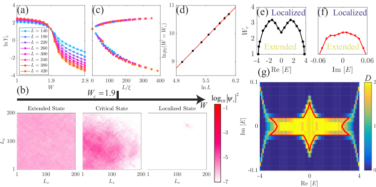
Figure 1: (a) $\ln Y_{L}$ vs $W$ for state of $E=0$. (b) Spatial distributions $\log_{10}|\Psi(x_{i},y_{i})|^{2}$ of wave function of state of $E=0$ in a typical realization for $W=1$ (extended), 1.9 (critical), and 5 (localized). The degree of red encodes the probability density as indicated by the color bar. (c) Scaling function $\ln[f(L/\xi)]$ vs $L/\xi$. (d) $\ln p_{2}(W=W_{c})$ as a function of $\ln L$. The solid line is a linear fit with slope $D=1.60\pm 0.05$. (e) $W_{c}$ vs $\text{Re}[E]$ for $\text{Im}[E]=0$. (f) $W_{c}$ vs $\text{Im}[E]$ for $\text{Re}[E]=0$. (g) Phase diagram in the complex eigenenergy plane $E$ at a fixed disorder strength $W$. Colour encodes the fractal dimension $D$. The red line is the mobility boundary with $D=1.6\pm 0.1$. Each point is averaged over 200 samples.

We first identify the ALTs from the finite-size scaling of the IPR. Similar to its Hermitian counterparts cwang2 , an ALT of system (1) occurs at a critical disorder strength $W_{c}$ at which all curves of $\ln Y_{L}(W)$ as a function $W$ for a state with given energy $E$ and for different system size $L$ cross as shown in Fig. 1(a) for $E=0$, $\gamma=\eta=0.1$ and $L$ ranging from 140 to 420. Indeed, data in Fig. 1(a) gives $W_{c}=1.90\pm 0.02$, and $d\ln Y_{L}(W)/dL$ is positive for $W<W_{c}$ and negative for $W>W_{c}$. These features clearly support the occurrence of an ALT: The state of $E=0$ is extended for $W<W_{c}$ and becomes localized for $W>W_{c}$. We also plot the wave functions distribution $\log_{10}|\psi_{i}|^{2}$ for three disorder strengths: $W=1<W_{c}$, $W=W_{c}$, and $W=5>W_{c}$, as shown in Fig. 1(b) where the degree of red color encodes probability density. Apparently, the wave function spread uniformly over the whole lattice at a length scale larger than $\xi$ for $W<W_{c}$ while it is highly localized on the lattice for $W>W_{c}$. At $W=W_{c}$, the state is critical that occupies a much sparser space than those of $W<W_{c}$ and resemble a fractal object xrwang1 .

The chi-square fit of $p_{2}(W)$ with a satisfactory goodness-of-fit of $Q=0.2$ yields the critical exponent $\nu=0.83\pm 0.06$, the fractal dimension of $D=1.60\pm 0.05$, the irrelevant exponent of $y=0.10\pm 0.03$, and $C=0.5\pm 0.1$. Fig. 1(c) shows the scaling functions of $f(x)$ obtained by collapsing all curves in Fig. 1(a) into a single one. We also plot $\ln p_{2}(W=W_{c})$ vs $\ln L$ in Fig. 1(d), and the curve is a straight line of a slope [fractal dimension] of $D=1.60\pm 0.05$ xrwang1 , the same value as that from the scaling function analysis. Interestingly, it agrees with an analytical result obtained from the non-Hermitian XY model telee3 .

The important feature or the fingerprint of a quantum phase transition is the universality concept. It says that critical exponents such as correlation length exponent $\nu$ and fractal dimension $D$ do not depend on model parameters. We carried out more calculations of IPR to show that $\nu$ and $D$ for the case without TR symmetry ($\eta=0.1$) do not depend (within numerical errors) on the strength of Rashba SOC $\alpha$, the complex eigenenergy $E$, and the form of disorders for $\gamma=0.1$. The results are summarized in Table 1.

Table 1: Critical exponent $\nu$, fractal dimension $D$ of wave functions at the ALT, and the goodness-of-fit $Q$ for different model parameters (Rashba SOC strength $\alpha$ and eigenenergy $E$) at a fixed non-Hermicity energy $\gamma=0.1$. We consider two different types of disorders: (i) Independent uniform distribution (as those in the main text) of $\epsilon_{i}$ in the window of $[-W/2,W/2]$; (ii) Independent Gaussian distribution (used in Ref. wwchen1 ) of $\epsilon_{i}$ with zero mean and the variance of $W^{2}$.

	$\nu$	$D$	$Q$
Uniform distribution
$E=0.0,\alpha=0.2$	$0.80\pm 0.05$	$1.65\pm 0.03$	0.1
$E=0.0,\alpha=0.3$	$0.7\pm 0.1$	$1.7\pm 0.1$	0.05
$E=0.01i,\alpha=0.1$	$0.6\pm 0.2$	$1.6\pm 0.1$	0.08
$E=0.1+0.01i,\alpha=0.1$	$0.85\pm 0.09$	$1.63\pm 0.8$	0.1
Gaussian distribution
$E=0.0,\alpha=0.1$	$0.8\pm 0.1$	$1.6\pm 0.2$	0.04

Figures 1(e) and (f) show how the critical disorder $W_{c}$ changes with the complex energy $E$: $W_{c}$ varies with $\text{Re}[E]$ for $\text{Im}[E]=0$ (e) and with $\text{Im}[E]$ for $\text{Re}[E]=0$ (f). All states are localized for $|\text{Re}[E]|>4$, and one needs the largest disorder strength (maximal $W_{c}$) to localize states around $\text{Re}[E]=\pm 1.6$. Different from its $\text{Re}[E]$-dependence, $W_{c}$ is monotonic in $|\text{Im}[E]|$.

The boundary that separates the extended states from the localized states is a closed curve in the complex energy plane as shown in Fig. 1(g) obtained from extensive numerical calculations of the IPR for different $E$ and system sizes $L$ (ranging from $L=160$ to $L=320$) at $W=2$. The wave functions at the mobility boundary (the red line in Fig. 1(g)) are fractals with the same fractal dimension $D=1.6$.

IV Level statistics

After establishing the ALTs for Hamiltonian (1), we are now in the position to discuss the level statistics of the extended states. Figures 2(a) and 2(d) are $P_{R}(s)$ (the cyan squares) and $P_{I}(s)$ (the purple cross) for systems without TR symmetry for $\eta=0.1$ (a) and with TR symmetry for $\eta=0$ (b) within $|E|<0.01$ for $L=160$, $W=1$, and $\gamma=0.1$, where all states are extended (see Fig. 1). Surprisingly, the level-spacing distribution of $\text{Re}[E]$ is well described by the Poisson function $P_{\text{P}}(s)$ no matter with or without the TR symmetry, instead of the Wigner-Dyson distributions of $P_{\beta=2}(s)$ or $P_{\beta=4}(s)$ that would be the case for an Hermitian Hamiltonian when $\gamma=0$. This is surprising because the Poisson distribution is not normally for extended states, but for the localized states whose eigenenergies distribute independently and randomly in certain energy ranges. Similarly, $P_{I}(s)$ is universally described by an unknown function in the sense that it does not depend on models with different forms of SOCs, disorders, and dimensionality, see Appendix B). This unknown function shows a “level repulsion”, i.e., $P_{I}(s=0)=0$.

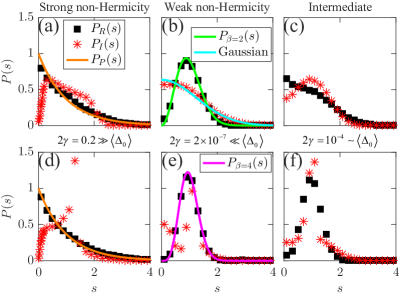
Figure 2: $P_{R}(s)$ (the cyan squares) and $P_{I}(s)$ (the purple cross) in the cases without TR symmetry for $\eta=0.1$ (a,b,c) and with TR symmetry for $\eta=0$ (d,e,f) within $|E|<0.01$ for $W=1$, $L=160$, and $\gamma=0.1$ (a,d), $\gamma=1\times 10^{-7}$ (b,e), and $\gamma=5\times 10^{-5}$ (c,f). The black solid lines in (a) and (d) are $P_{\text{P}}(s)$. The red and the orange solid lines in (b) and (e) are $P_{\beta=2}(s)$ and $P_{\beta=4}(s)$, respectively. The green solid line in (b) is the Gaussian function.

However, for very small non-Hermicity of $\gamma=10^{-7}$ and the same $W=1$ and $L=160$, $P_{R}(s)$, obtained from those extended states within the window of $|E|<0.01$, follows perfectly with the Wigner-Dyson distributions of $P_{\beta=2}(s)$ and $P_{\beta=4}(s)$ as shown in Figs. 2(b) and 2(e), respectively for the cases without and with TR symmetry. At the same time, $P_{I}(s)$ is universally described by the Gaussian function for $\eta\neq 0$ or by an unknown function with a universal non-zero constant $P_{I}(s=0)$, or non-level-repulsion, in the sense that the distribution are model-independent, see Appendix B. For the intermediate non-Hermicity energy of $2\gamma=10^{-4}$, some parameter-dependent distributions of $P_{R}(s)$ and $P_{I}(s)$ are seen, as shown in Fig. 2(c) for $\eta=0.1$ and 2(f) for $\eta=0$.

To obtain the insight of the dramatical change in level statistics from the Wigner-Dyson distribution of $\gamma=0$ to the Poisson distribution of non-zero $\gamma$, we follow the wisdom of Wigner by considering the two-by-two non-Hermitian random matrix mlmehta1

$$\begin{gathered}\mathcal{H}=\begin{bmatrix}\epsilon_{1}+\epsilon_{2}&h_{12}\\ h_{21}&\epsilon_{1}-\epsilon_{2}\end{bmatrix}+i\gamma\sigma_{z}.\end{gathered}$$ (3)

$\epsilon_{1,2}$ and $h_{12}$ are independent random variants of Gaussian distribution of zero mean and variance $\sigma^{2}$, i.e., $f(x,\sigma)\sim\exp[-x^{2}/\sigma^{2}]$. $\gamma$ is of the non-Hermicity energy. Hamiltonian (3) breaks both spin-rotation symmetry and TR symmetry. The difference of the two eigenenergies (level spacing) is

$$\begin{gathered}\Delta=\sqrt{\Delta^{2}_{0}-4\gamma^{2}+i8\gamma\epsilon_{2}},\end{gathered}$$ (4)

with $\Delta_{0}=2\sqrt{\epsilon^{2}_{2}+|h_{12}|^{2}}$ being the mean level spacing of the Hermitian part of Hamiltonian (3). If $\gamma=0$, the eigenenergies are real, and its level spacing distribution is $P(s)=\int\delta(s-\Delta_{0})\exp[-(\epsilon_{2}^{2}+|h_{12}|^{2})/\sigma^{2}]d\epsilon_{2}d^{\beta}h_{12}$, where $\Delta_{0}=\sqrt{\epsilon_{2}^{2}+|h_{12}|^{2}}$, $|h_{12}|^{2}=\xi_{1}^{2};\ \ \xi_{1}^{2}+\xi_{2}^{2};\ \ \xi_{1}^{2}+\xi_{2}^{2}+\xi_{3}^{2}+\xi_{4}^{2}$ for the Gaussian orthogonal ensemble ($\beta=1$, real matrix elements), the Gaussian unitary ensemble ($\beta=2$, complex matrix elements), and the Gaussian symplectic ensemble ($\beta=4$, quaternion matrix elements) respectively. Here $\xi_{i}$ ($i=1,2,3,4$) are real. Thus, $P(s)=C_{1}s^{\beta}\exp[-C_{2}s^{2}]$ is exactly the well-known Wigner-Dyson distribution. The prefactor is proportional to the area of equal-$\Delta_{0}$ hyper-surface in the $\epsilon_{2}-\vec{\xi}$ space. If $\gamma=0$ in the current case, level spacing $\Delta=\Delta_{0}$ is non-negative. Any coupling (non-zero $\xi_{1}$ and $\xi_{2}$) tends to push two levels apart. The probability of having zero level spacing is the probability to have $\epsilon_{2}=\xi_{1}=\xi_{2}=0$, which is vanishingly small and gives rise to the Wigner-Dyson distributions. However, if $|\gamma|$ is of the order of $\Delta_{0}$, the real part of $\Delta$ is possible to be negative, zero, and positive. In this case, two levels can freely cross each other, and are, in principle, independent from each other. This is our understanding of why $P_{R}(s)$ follows the Poisson function (see derivation later).

Above poor-man’s analysis reveals two relevant energy scales for the level statistics: The mean level spacing $\langle\Delta_{0}\rangle$ of the Hermitian part of the model and the non-Hermicity energy $2\gamma$. We expect three different regimes. (i) Strong non-Hermicity limit $2\gamma\gg\langle\Delta_{0}\rangle$: Level repulsion is invalid, and two quasiparticle levels can freely cross each other such that the quasiparticle level spacing distribution follow the universal Poisson function that is for independent random level distribution. The spacings of the imaginary part of the complex eigenenergies follow an unknown universal distribution function. (ii) Weak non-Hermicity limit $2\gamma\ll\langle\Delta_{0}\rangle$: The non-Hermicity energy is much smaller than the average level spacings between two Hermitian modes. Therefore, the non-Hermicity is not enough to induce level crossing so that quasiparticle level spacing of extended states follows still the Wigner-Dyson statistics. (iii) Intermediate non-Hermicity: The level spacings follow some non-universal distributions that are sensitive to the details of a model. This explains well the changes of level statistics when the ratio of non-Hermicity energy to $\langle\Delta_{0}\rangle$ is tuned by fixing lattice size $L$ and varying $\gamma$.

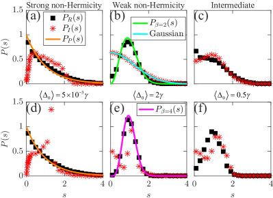
Figure 3: $P_{R}(s)$ (cyan squares) and $P_{I}(s)$ (purple cross) within $|E|<0.01$ in the cases of TR-broken ((a,b,c) for $\eta=0.1$) and TR-preservation ((d,e,f) for $\eta=0$) for $\gamma=10^{-2}$, $W=1$, and $L=200$ (a,d), $L=10$ (b,e), and $L=20$ (c,f). The black solid lines in (a) and (d) are $P_{\text{P}}(s)$. The red and the orange solid lines in (b) and (e) are $P_{\beta=2}(s)$ and $P_{\beta=4}(s)$, respectively. The green solid line in (b) is the Gaussian function.

We further verify above picture by noticing that the ratio of non-Hermicity energy to $\langle\Delta_{0}\rangle$ can also be tuned by fixing $\gamma$ and varying lattice size $L$ because the mean level spacing is inversely proportional to the number of lattice sites as $\langle\Delta_{0}\rangle\simeq 0.22(W+8)/L^{2}$, see Appendix C for the clarification. We compute $P_{R}(s)$ and $P_{I}(s)$ in the energy range of $|E|<0.01$ for the cases with and without TR symmetry and for $W=1$, $\gamma=10^{-2}$ and three different system sizes: $L=200$ ($\langle\Delta_{0}\rangle=5\times 10^{-3}\gamma$), $L=20$ ($\langle\Delta_{0}\rangle=0.5\gamma$), and $L=10$ ($\langle\Delta_{0}\rangle=2\gamma$). The results are plotted in Fig. 3 for the cases with (a,b,c) and without (d,e,f) TR symmetry. Similar to the results for the cases of fixing $L$ and varying $\gamma$ above, $P_{R}(s)$ follows either the Poisson or Wigner-Dyson distribution while $P_{I}(s)$ follows either an unknown universal or the Gaussian distribution when lattice size are respectively of $L=200$ and $L=10$). It should be noted that the system is always in the strong non-Hermicity limit at fixed $\gamma\neq 0$ and in the thermodynamic limit of $L\rightarrow\infty$ so that the quasiparticle energy level spacing distribution is Poissonian. All our results show that analysis based on the random matrix (3) can explain the results shown in Figs. 2 and 3 for strong and weak non-Hermicity limits.

Before ending this section, we would like to point out that the Poisson level statistics is universal for all systems without level repulsion, i.e. level cross each other independently as what was recently observed in non-Hermitian systems mharder1 ; klaui ; skkim ; cmhu . If levels can freely cross, then the probability to find a nearest neighbouring level located within $[s,s+\delta s]$ is the product of the probability of no level within $[0,s]$ with the probability of the level falling in $[s,s+\delta s]$, i.e. $P(s)\delta s=(1-\int_{0}^{s}P(s^{\prime})ds^{\prime})\delta s/\Delta$, where $\Delta$ is the mean level spacing. Thus, $P(s)$ satisfies differential equation of $\frac{dP}{ds}=-P/\Delta$ whose solution is just the Poisson function. When $\Delta$ is used as the unit of level spacing, $P(s)$ is exactly what we found in this paper.

V Discussion

There are some very recent studies of the level statistics of non-Hermitian systems. Hamazaki et al have also observed the Poisson distribution of $P_{R}(s)$ in a non-Hermitian many-body Hamiltonian with the TR symmetry rhamazaki1 . On the other hand, a non-Hermitian type level repulsion is witnessed by studying the distribution of spacings of two nearest neighbor eigenvalues in the complex energy space aftzortzakakis1 ; yhuang1 . Moreover, a new universal level statistics at metal-insulator transition is conjectured. These papers indeed studied the similar issue, but did not obtain the central results in this work, i.e., the universal Poisson distribution of $P_{R}(s)$ and $P_{I}(s)$ in both strong and weak non-Hermicity limits. Obviously, our results offer a way to manipulate energy levels. For example, one may change the relative position of two levels by active level repulsion or level crossing through controlling the strength of non-Hermicity, a concept of damping engineering.

Pertaining to the relevance of the reality, the Hermitian part of Hamiltonian  (1) is usually used to describe 2DEGs of semiconductors heterostructures with Rashba SOCs tando1 . The non-Hermicity term $i\gamma\sigma_{z}$ with an additional non-Hermitian on-site energy $-i\gamma_{0}\sigma_{0}$ ($\gamma_{0}>|\gamma|$) can arise from the spin dependent lifetimes due to the omnipresent electron-electron, electron-impurity, and electron-phonon interactions vkozii1 ; hshen1 ; aazyuzin1 ; mpapaj1 , if the semiconductors heterostructures are magnetic. In principle, the additional term $-i\gamma_{0}\sigma_{0}$ does not change the level statistics discussed here, see the proof in Appendix D. Furthermore, Rashba SOCs can emerge in cold-atomic amanchon ; gorso1 , photonics llu1 , magnonic yonose ; xswang , and skyrmionic systems hyang1 ; zxli . All these systems can be described by very similar non-Hermitian Hamiltonians due to the inevitable gain/loss in open systems.

VI Conclusion

In conclusion, 2DEGs subjected to an imaginary magnetic field, random on-site energies, and SOCs undergo an ALT at a finite disorder $W_{c}$. Near $W_{c}$, correlation lengths diverge as $\xi(W)\propto|W-W_{c}|^{-\nu}$ with $\nu=0.83\pm 0.05$. A mobility boundary separating the extended from the localized states exists in the complex energy plane. In the thermodynamic limit of infinity system size, the quasiparticle level spacing $P_{R}(s)$ in the metallic phase is universally described by the Poisson distribution no matter whether the system has the time-reversal symmetry or not, while the spacing of the imaginary part of the complex eigenenergies $P_{I}(s)$ is also universal, exhibits “level repulsion”, and is sensitive to the TR symmetry. For a finite system when the non-Hermicity energy $\gamma$ is smaller than the mean level spacing, $P_{R}(s)$ can be described by the Wigner-Dyson distribution $P_{\beta}(s)$ and $P_{I}(s)$ is universal with a universal non-zero constant.

VII Acknowledgments

This work is supported by the National Natural Science Foundation of China (Grants No. 11774296, 11704061, and 11974296) and Hong Kong RGC (Grants No. 16301518, 16301619 and 16300117). C.W. is supported by UESTC and the China Postdoctoral Science Foundation (Grants No. 2017M610595 and 2017T100684). C.W. also acknowledges the kindly help from Xiansi Wang and Jie Lu.

Appendix A Finite-size scaling analysis

To extract the fractal dimension, the critical disorder, and the critical exponent $\nu$ at the quantum phase transitions defined in the scaling function Eq. (2) with $\xi=\xi_{0}|W-W_{c}|^{-\nu}$, i.e.,

$$\begin{gathered}p_{2}(L,W)=L^{D}[f(L|W-W_{c}|^{\nu}/\xi_{0})+CL^{-y}],\end{gathered}$$ (5)

we perform a Taylor expansion of the scaling function $f(x)$ up to the third order in $|W-W_{c}|^{\nu}$ near $W=W_{c}$,

$$\begin{gathered}f(L|W-W_{c}|^{\nu}/\xi_{0})=F_{0}+F_{1}L|W-W_{c}|^{\nu}/\xi_{0}+F_{2}(L|W-W_{c}|^{\nu}/\xi_{0})^{2}+F_{3}(L|W-W_{c}|^{\nu}/\xi_{0})^{3}\\ =F_{0}+\tilde{F}_{1}L|W-W_{c}|^{\nu}+\tilde{F}_{2}(L|W-W_{c}|^{\nu})^{2}+\tilde{F}_{3}(L|W-W_{c}|^{\nu})^{3},\end{gathered}$$ (6)

with $D,C,y,\nu,W_{c},F_{0},\tilde{F}_{1},\tilde{F}_{2},\tilde{F}_{3}$ being fitting parameters. Then we adjust those parameters to minimize the chi square

$$\begin{gathered}\chi^{2}=\sum^{N_{w}}_{i}\sum^{N_{l}}_{j}\left(\dfrac{p_{2}(W_{i},L_{j})-L^{D}_{j}[f(L_{j}|W_{i}-W_{c}|^{\nu}/\xi_{0})+CL^{-y}_{j}]}{\sigma_{ij}}\right)\end{gathered}$$ (7)

following the approach illustrated in the appendix of Ref. wwchen1 , where $N_{w}$ and $N_{e}$ are the number of $W$ and $L$, respectively. The fitting process yields the critical disorder $W_{c}$, the fractal dimension $D$, and the critical exponent $\nu$. After determining the minimal chi square, we calculate the goodness-of-fit $Q$ by the standard algorithm suggested in Ref. numerical , which measures how well our numerical data of $p_{2}$ fit to the model of Eq. (5). Take data in Fig. 1(a) as examples: Following the above process, we obtain $Q=0.2>10^{-3}$, a satisfactory number that says the fit acceptable.

Appendix B Model-independence of level statistics

To demonstrate that $P_{R}(s)$ and $P_{I}(s)$ are universal in the strong and weak non-Hermicity limits, we study level statistics of extended states for other random non-Hermitian models with different forms of SOCs, disorders, and dimensionality.

Firstly, we study Hamiltonian  (1) with different forms of SOCs. The first one is the random SU(2) model subjected to an imaginary perpendicular magnetic field $(0,0,i\gamma)$ cwang ,

$$\begin{gathered}H=\sum_{i}c^{\dagger}_{i}(\epsilon_{i}\sigma_{0}+\eta\sigma_{z}+i\gamma\sigma_{z})c_{i}+\left(t\sum_{\langle ij\rangle}c^{\dagger}_{i}V_{ij}c_{j}+h.c.\right),\end{gathered}$$ (8)

with

$$\begin{gathered}V_{ij}=\begin{bmatrix}e^{-i\alpha_{ij}}\cos(\beta_{ij}/2)&e^{-i\gamma_{ij}}\sin(\beta_{ij}/2)\\ e^{i\gamma_{ij}}\sin(\beta_{ij}/2)&e^{i\alpha_{ij}}\cos(\beta_{ij}/2).\end{bmatrix}.\end{gathered}$$ (9)

Here $\alpha_{ij}$ and $\gamma_{ij}$ distribute randomly and uniformly in the range of $[0,2\pi)$. $\sin(\beta_{ij}/2)$ distributes uniformly in $[0,1)$. The second model is to replace the Rashba SOC in model 1 by the Dresselhaus SOC gdresselhaus , where the matrices $V_{ij}$ are parametrized as $V_{x}$ and $V_{y}$ for the $x-$ and the $y-$direction hopping, respectively,

$$\begin{gathered}V_{x}=\sigma_{0}+i\zeta\sigma_{x},V_{y}=\sigma_{0}-i\zeta\sigma_{y}.\end{gathered}$$ (10)

Here the constant $\zeta$ measures the strength of the Dresselhaus SOC.

The case without TR symmetry ($\eta=0.1$) and the case with TR symmetry ($\eta=0$) are investigated. $P_{R}(s)$ and $P_{I}(s)$ within the energy window of $|E|<0.01$ for $W=1$, $L=160$, and $\gamma=0.1$ (strong non-Hermicity limit) or $\gamma=10^{-7}$ (weak non-Hermicity limit) for all three models are plotted in Fig. 4. It is clear that all three models (Rashba, Dresselhaus and random SU(2) SOCs) give identical $P_{R}(s)$ and $P_{I}(s)$. Within the symbol size, we cannot see any difference in both $P_{R}(s)$ and $P_{I}(s)$ for all three models. Thus, these results provide strong evidence that the new distributions are independent of the forms of SOCs.

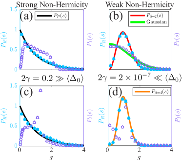
Figure 4: $P_{R}(s)$ (the filled symbols) and $P_{I}(s)$ (the open symbols) within $|E|<0.01$ in the cases without TR symmetry ((a,b) for $\eta=0.1$) and with TR symmetry ((c,d) for $\eta=0$) for $W=1$, $L=160$, and $\gamma=0.1$ (a,c), $\gamma=1\times 10^{-7}$ (b,d). The black solid lines in (a) and (c) are $P_{\text{P}}(s)$. The red and the orange solid lines in (b) and (d) are $P_{\beta=2}(s)$ and $P_{\beta=4}(s)$, respectively. The green solid line in (b) is the Gaussian function. The squares, triangles and circles are respectively for the Rashba SOC, the Dresselhaus SOC, and the SU(2) SOC.

Secondly, we show that the level statistics do not depend on the forms of disorders by considering the following model,

$$\begin{gathered}H=\sum_{\bm{i}}c^{\dagger}_{\bm{i}}(\epsilon_{\bm{i}}\sigma_{0}+\eta\sigma_{z}+i\gamma_{\bm{i}}\sigma_{z})c_{\bm{i}}+\sum_{\langle\bm{ij}\rangle}c^{\dagger}_{\bm{i}}V_{\bm{ij}}c_{\bm{i}}+h.c.,\end{gathered}$$ (11)

where $\epsilon_{\bm{i}}$ and $\gamma_{\bm{i}}$ are independent random numbers that distribute in the range of $[-W/2,W/2]$ and $[-\Gamma/2,\Gamma/2]$, respectively. $V_{\bm{ij}}=V_{x}=\sigma_{0}+i\alpha\sigma_{y}$ and $V_{y}=\sigma_{0}-i\alpha\sigma_{x}$ for $\langle\bm{ij}\rangle$ along the $x-$ and the $y-$directions. $\alpha$ and $\eta$ are two constants measuring SOC strength and the degree of TR symmetry violation. Different from model (1) with the constant non-Hermicity, both the Hermitian and the non-Hermitian parts are random here. All states of this model within the energy window of $|E|<0.01$ for $W=1$, $\alpha=\eta=0.1$, $L=160$ (system sizes), and $\Gamma=0.1$ (strong non-Hermicity) and $10^{-7}$ (weak non-Hermicity) are extended. The corresponding $P_{R}(s)$ and $P_{I}(s)$ of those states are plotted in Figs. 5 ($\eta=0.1$, without TR symmetry) and 6 ($\eta=0$, with TR symmetry). They are the same as those of Model (8).

Figure 5: Results of Hamiltonian (11) without TR symmetry ($\eta=0.1$). (a-c) Strong Non-Hermicity $\Gamma=0.1$: (a) $\ln p_{2}(E=0)$ as a function of $\ln L$. The red dash line is a linear fit with slope $D=1.99\pm 0.01$. (b) $P_{R}(s)$ (the black squares) within $|E|<0.01$. The orange solid line is $P_{\text{P}}(s)$. (c) $P_{I}(s)$ within $|E|<0.01$ for Hamiltonian (11) (the filled squares) and for Hamiltonian (1) (the empty squares). (d-f) Weak Non-Hermicity $\Gamma=10^{-7}$: (d) $\ln p_{2}(E=0)$ as a function of $\ln L$. The red dash line is a linear fit with slope $D=1.99\pm 0.01$. (e) $P_{R}(s)$ (the black squares) within $|E|<0.01$. The green solid line is $P_{\beta=2}(s)$. (f) $P_{I}(s)$ within $|E|<0.01$ for Hamiltonian (11) (the filled squares) and for Hamiltonian (1) (the empty squares). The cyan solid line is the Gaussian function.

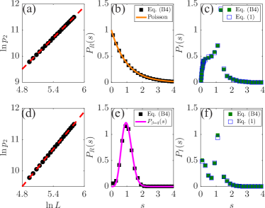
Figure 6: Results of Hamiltonian (11) with TR symmetry ($\eta=0$). (a-c) Strong Non-Hermicity $\Gamma=0.1$: (a) $\ln p_{2}(E=0)$ as a function of $\ln L$. The red dash line is a linear fit with slope $D=1.99\pm 0.01$. (b) $P_{R}(s)$ (the black squares) within $|E|<0.01$. The orange solid line is $P_{\text{P}}(s)$. (c) $P_{I}(s)$ within $|E|<0.01$ for Hamiltonian (11) (the filled squares) and for Hamiltonian (1) (the empty squares). (d-f) Weak Non-Hermicity $\Gamma=10^{-7}$: (d) $\ln p_{2}(E=0)$ as a function of $\ln L$. The red dash line is a linear fit with slope $D=1.99\pm 0.01$. (e) $P_{R}(s)$ (the black squares) within $|E|<0.01$. The magenta solid line is $P_{\beta=4}(s)$. (f) $P_{I}(s)$ within $|E|<0.01$ for Hamiltonian (11) (the filled squares) and for Hamiltonian (1) (the empty squares).

Thirdly, we investigate the level statistics of a three-dimensional non-Hermitian Anderson model

$$\begin{gathered}H=\sum_{\bm{i}}c^{\dagger}_{\bm{i}}(\epsilon_{\bm{i}}+i\theta_{\bm{i}})c_{\bm{i}}+t\sum_{\langle\bm{ij}\rangle}c^{\dagger}_{\bm{i}}c_{\bm{j}}+h.c.,\end{gathered}$$ (12)

where $c^{\dagger}_{\bm{i}}$ and $c_{\bm{i}}$ are the creation and annihilation operator of a single electron at site $\bm{i}=(l,m,n)$ with $l,m,n$ being integers and $1\leq l,m,n\leq L$. The hopping energy $t$ is chosen as the energy unit, i.e., $t=1$. Randomness is introduced through random real numbers $\epsilon_{\bm{i}}$ and $\theta_{\bm{i}}$ uniformly and independently distributed in $[-W/2,W/2]$ and $[-\Theta/2,\Theta/2]$, respectively. Periodic boundary conditions are applied in all directions to avoid the non-Hermitian skin effect. The obtained $P_{R}(s)$ and $P_{I}(s)$ in the energy interval of $|E|\in[-0.01,0.01]$ and $W=1$ are shown in Fig. 7. Clearly, they also follow the same level statistics as those of states of Hamiltonian (1).

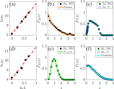
Figure 7: Results of Hamiltonian (12). (a-c) Strong Non-Hermicity $\Theta=0.1$: (a) $\ln p_{2}(E=0)$ as a function of $\ln L$. The red dash line is a linear fit with slope $D=3.01\pm 0.01$. (b) $P_{R}(s)$ (the black squares) within $|E|<0.01$. The orange solid line is $P_{\text{P}}(s)$. (c) $P_{I}(s)$ within $|E|<0.01$ for Hamiltonian (12) (the filled squares) and for Hamiltonian (1) (the empty squares). (d-f) Weak Non-Hermicity $\Theta=10^{-7}$: (d) $\ln p_{2}(E=0)$ as a function of $\ln L$. The red dash line is a linear fit with slope $D=2.98\pm 0.01$. (e) $P_{R}(s)$ (the black squares) within $|E|<0.01$. The green solid line is $P_{\beta=2}(s)$. (f) $P_{I}(s)$ within $|E|<0.01$ for Hamiltonian (12) (the filled squares) and for Hamiltonian (1) (the empty squares). The cyan solid line is the Gaussian function.

Appendix C Mean level spacing of Hermitian part

The mean level spacing $\langle\Delta_{0}\rangle$ of the Hermitian part of Hamiltonian (1) is an important energy scale related different level statistics. In this section, we want to find an accurate estimate of $\langle\Delta_{0}\rangle$ for a given system size $L$ and disorder strength $W$. For small disorders $W$, all eigenenergies should lie in the energy range of $[-(4+W/2),(4+W/2)]$ such that the energy bandwidth is about $8+W$. Since the number of eigenstates is proportional to $L^{2}$, the mean level spacing should then satisfy

$$\begin{gathered}\langle\Delta_{0}\rangle=\beta\dfrac{(W+8)}{L^{2}},\end{gathered}$$ (13)

with $\beta$ being a coefficient that is obtained below.

To numerically determine the coefficient $\beta$, we calculate $\langle\Delta_{0}\rangle$ and plot them (symbols) against $L$ in Fig. 8. Here $\Delta_{0}$ is obtained from a small energy window $[-0.01,0.01]$ around $E=0$, and $\langle\cdots\rangle$ is averaged over more than 200 ensembles. A fit of $\langle\Delta_{0}\rangle$ to Eq. (13) yields $\beta\simeq 0.22$, which accords well with numerical data (up to $L=200$), see the black line in Fig. 8. Thus, the mean level spacing of the Hermitian part of Hamiltonian (1) can be obtained by formula $\langle\Delta_{0}\rangle\simeq 0.22(W+8)/L^{2}$.

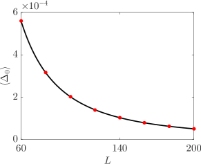
Figure 8: Mean level spacings $\langle\Delta_{0}\rangle$ (the red circles) of the Hermitian part of Hamiltonian (1) as a function of $L$ for $W=1$. The black line is Eq. (13) with $\beta=0.22$. Each point is averaged over more than 200 ensembles.

Appendix D Level statistics of Hamiltonian (1) with an additional term

We show that an additional term of $-i\gamma_{0}\sigma_{0}$ to Hamiltonian (1), i.e., $\tilde{H}=H-\sum_{\bm{i}}c^{\dagger}_{\bm{i}}\gamma_{0}\sigma_{0}c_{\bm{i}}$, does not affect $P_{R}(s)$ and $P_{I}(s)$. Suppose $|\psi_{E}\rangle$ is an arbitrary right eigenstate of Hamiltonian $H$ with eigenenergy $E$, then

$$\begin{gathered}\tilde{H}|\psi_{E}\rangle=\left(H-\sum_{\bm{i}}c^{\dagger}_{\bm{i}}\gamma_{0}\sigma_{0}c_{\bm{i}}\right)|\psi_{E}\rangle\\ =(H-i\gamma_{0}I)|\psi_{E}\rangle=(E-i\gamma_{0})|\psi_{E}\rangle\end{gathered}$$ (14)

with $I$ being the identity matrix. Thus, $|\psi_{E}\rangle$ is also a right eigenstate of $\tilde{H}$ with eigenenergy $E-i\gamma_{0}$. Since $|\psi_{E}\rangle$ is arbitrary, all the levels of $\tilde{H}$ are the same as those of $H$ but shift by a constant imaginary value of $-i\gamma_{0}$. Obviously, the constant shift of all levels of complex energies does not change the distributions of level spacings, $P_{R}(s)$ and $P_{I}(s)$.

References

- (1) H. J. Carmichael, Quantum Trajectory Theory for Cascaded Open Systems, Phys. Rev. Lett. 70, 2273 (1993).
- (2) N. Hatano and D. R. Nelson, Localization Transitions in Non-Hermitian Quantum Mechanics, Phys. Rev. Lett. 77, 570 (1996).
- (3) N. M. Shnerb and D. R. Nelson, Winding Numbers, Complex Currents, and Non-Hermitian Localization, Phys. Rev. Lett. 80, 5172 (1998).
- (4) K. G. Makris, R. El-Ganainy, D. N. Christodoulides, and Z. H. Musslimani, Beam Dynamics in Symmetric Optical Lattices, Phys. Rev. Lett. 100, 103904 (2008).
- (5) S. Klaiman, U. Günther, and N. Moiseyev, Visualization of Branch Points in -Symmetric Waveguides, Phys. Rev. Lett. 101, 080402 (2008).
- (6) S. Longhi, Bloch Oscillations in Complex Crystals with Symmetry, Phys. Rev. Lett. 103, 123601 (2009).
- (7) C. E. Rüter, K. G. Makris, R. El-Ganainy, D. N. Christodoulides, M. Segev, and D. Kip, Observation of Parity–Time Symmetry in Optics, Nat. Phys. 6, 192 (2010).
- (8) Y. Choi, S. Kang, S. Lim, W. Kim, J.-R. Kim, J.-H. Lee, and K. An, Quasieigenstate Coalescence in an Atom-Cavity Quantum Composite, Phys. Rev. Lett. 104, 153601 (2010).
- (9) S. Diehl, E. Rico, M. A. Baranov, and P. Zoller, Topology by Dissipation in Atomic Quantum Wires, Nat. Phys. 7, 971 (2011).
- (10) S. Bittner, B. Dietz, U. Günther, H. L. Harney, M. Miski-Oglu, A. Richter, and F. Schäfer, Symmetry and Spontaneous Symmetry Breaking in a Microwave Billiard, Phys. Rev. Lett. 108, 024101 (2012).
- (11) A. Regensburger, C. Bersch, M.-A. Miri, G. Onishchukov, D. N. Christodoulides, and U. Peschel, Parity–Time Synthetic Photonic Lattices, Nature (London) 488, 167 (2012).
- (12) L. Chang, X. Jiang, S. Hua, C. Yang, J. Wen, L. Jiang, G. Li, G. Wang, and M. Xiao, Parity–Time Symmetry and Variable Optical Isolation in Active–Passive-Coupled Microresonators, Nat. Photonics 8, 524 (2014).
- (13) B. Peng, Ş. K. Özdemir, S. Rotter, H. Yilmaz, M. Liertzer, F. Monifi, C. M. Bender, F. Nori, and L. Yang, Loss Induced Suppression and Revival of Lasing, Science 346, 328 (2014).
- (14) L. Feng, Z. J. Wong, R.-M. Ma, Y. Wang, and X. Zhang, Single-Mode Laser by Parity-Time Symmetry Breaking, Science 346, 972 (2014).
- (15) H. Hodaei, M.-A. Miri, M. Heinrich, D. N. Christodoulides, and M. Khajavikhan, Parity-Time–Symmetric Microring Lasers, Science 346, 975 (2014).
- (16) T. E. Lee, F. Reiter, and N. Moiseyev, Entanglement and Spin Squeezing in Non-Hermitian Phase Transitions, Phys. Rev. Lett. 113, 250401 (2014).
- (17) H. Cao and J. Wiersig, Dielectric Microcavities: Model Systems for Wave Chaos and Non-Hermitian Physics, Rev. Mod. Phys. 87, 61 (2015).
- (18) B. Zhen, C. W. Hsu, Y. Igarashi, L. Lu, I. Kaminer, A. Pick, S.-L. Chua, J. D. Joannopoulos, and M. Soljačić, Spawning Rings of Exceptional Points out of Dirac Cones, Nature 525, 354 (2015).
- (19) T. Gao, E. Estrecho, K. Y. Bliokh, T. C. H. Liew, M. D. Fraser, S. Brodbeck, M. Kamp, C. Schneider, S. Höfling, Y. Yamamoto et al., Observation of Non-Hermitian Degeneracies in a Chaotic Exciton-Polariton Billiard, Nature 526, 554 (2015).
- (20) S. Malzard, C. Poli, and H. Schomerus, Topologically Protected Defect States in Open Photonic Systems with Non-Hermitian Charge-Conjugation and Parity-Time Symmetry, Phys. Rev. Lett. 115, 200402 (2015).
- (21) K. Esaki, M. Sato, K. Hasebe, and M. Kohmoto, Edge States and Topological Phases in Non-Hermitian Systems, Phys. Rev. B 84, 205128 (2011).
- (22) S.-D. Liang and G.-Y. Huang, Topological Invariance and Global Berry Phase in Non-Hermitian Systems, Phys. Rev. A 87, 012118 (2013).
- (23) T. E. Lee, Anomalous Edge State in a Non-Hermitian Lattice, Phys. Rev. Lett. 116, 133903 (2016).
- (24) D. Leykam, K. Y. Bliokh, C. Huang, Y. D. Chong, and F. Nori, Edge Modes, Degeneracies, and Topological Numbers in Non-Hermitian Systems, Phys. Rev. Lett. 118, 040401 (2017).
- (25) Y. Xu, S.-T. Wang, and L.-M. Duan, Weyl Exceptional Rings in a Three-Dimensional Dissipative Cold Atomic Gas, Phys. Rev. Lett. 118, 045701 (2017).
- (26) H. Menke and M. M. Hirschmann, Topological Quantum Wires with Balanced Gain and Loss, Phys. Rev. B 95, 174506 (2017).
- (27) Y. Xiong, Why Does Bulk Boundary Correspondence Fail in Some Non-Hermitian Topological Models, arXiv:1705.06039.
- (28) V. Kozii and L. Fu, Non-Hermitian Topological Theory of Finite-Lifetime Quasiparticles: Prediction of Bulk Fermi Arc Due to Exceptional Point, arXiv:1708.05841.
- (29) A. A. Zyuzin and A. Yu. Zyuzin, Flat Band in Disorderdriven Non-HermitianWeyl Semimetals, Phys. Rev. B 97, 041203(R) (2018).
- (30) V. M. Martinez Alvarez, J. E. Barrios Vargas, and L. E. F. Foa Torres, Non-Hermitian Robust Edge States in One Dimension: Anomalous Localization and Eigenspace Condensation at Exceptional Points, Phys. Rev. B 97, 121401(R) (2018).
- (31) C. Li, X. Z. Zhang, G. Zhang, and Z. Song, Topological Phases in a Kitaev chain with Imbalanced Pairing, Phys. Rev. B 97, 115436 (2018).
- (32) H. Shen, B. Zhen, and L. Fu, Topological Band Theory for Non-Hermitian Hamiltonians, Phys. Rev. Lett. 120, 146402 (2018).
- (33) S. Yao and Z. Wang, Edge States and Topological Invariants of Non-Hermitian Systems, Phys. Rev. Lett. 121, 086803 (2018).
- (34) S. Yao, F. Song, and Z. Wang, Non-Hermitian Chern Bands, Phys. Rev. Lett. 121, 136802 (2018).
- (35) Z. Gong, Y. Ashida, K. Kawabata, K. Takasan, S. Higashikawa, and M. Ueda, Topological Phases of Non-Hermitian Systems, Phys. Rev. X 8, 031079 (2018).
- (36) X. Ni, D. Smirnova, A. Poddubny, D. Leykam, Y. Chong, and A. B. Khanikaev, Phase Transitions of Edge States at Symmetric Interfaces in Non-Hermitian Topological Insulators, Phys. Rev. B 98, 165129 (2018).
- (37) T. M. Philip, M. R. Hirsbrunner, and M. J. Gilbert, Loss of Hall Conductivity Quantization in a Non-Hermitian Quantum Anomalous Hall Insulator, Phys. Rev. B 98, 155430 (2018).
- (38) Y. Chen and H. Zhai, Hall Conductance of a Non-Hermitian Chern Insulator, Phys. Rev. B 98, 245130 (2018).
- (39) C. Wang and X. R. Wang, Non-Quantized Edge Channel Conductance and Zero Conductance Fluctuation in Non-Hermitian Chern Insulators, arXiv:1901.06982.
- (40) M. Papaj, H. Isobe, and L. Fu, Nodal Arc of Disordered Dirac Fermions and Non-Hermitian Band Theory, Phys. Rev. B 99, 201107(R) (2019).
- (41) M. L. Mehta, Random Matrices (Elsevier, Amsterdam, 2004).
- (42) F. Haake, Quantum signatures of chaos (Springer Science & Business Media, 2010).
- (43) C. Poli, G. A. Luna-Acosta, and H.-J. Stöckmann, Nearest Level Spacing Statistics in Open Chaotic Systems: Generalization of the Wigner Surmise, Phys. Rev. Lett. 108, 174101 (2012).
- (44) R. Hamazaki, K. Kawabata, and M. Ueda, Non-Hermitian Many-Body Localization, Phys. Rev. Lett. 123, 090603 (2019).
- (45) A. F. Tzortzakakis, K. G. Makris, and E. N. Economou, Non-Hermitian disorder in two-dimensional optical lattices, Phys. Rev. B 101, 014202 (2020).
- (46) Y. Huang and B. I. Shklovskii, Anderson transition in three-dimensional systems with non-Hermitian disorder, Phys. Rev. B 101, 014204 (2020).
- (47) M. Harder, Y. Yang, B. M. Yao, C. H. Yu, J. W. Rao, Y. S. Gui, R. L. Stamps, and C.-M. Hu, Level Attraction Due to Dissipative Magnon-Photon Coupling, Phys. Rev. Lett. 121, 137203 (2018).
- (48) I. Boventer, C. Dörflinger, T. Wolz, R. Macêdo, R. Lebrun, M. Kläui, and M. Weides, Control of the coupling strength and linewidth of a cavity magnon-polariton, Phys. Rev. Research 2, 013154 (2020).
- (49) B. Bhoi, B. Kim, S.-H. Jang, J. Kim, J. Yang, Y.-J. Cho, and S.-K. Kim, Abnormal anticrossing effect in photon-magnon coupling, Phys. Rev. B 99, 134426 (2019).
- (50) Y. Yang, J.W. Rao, Y.S. Gui, B.M. Yao, W. Lu, and C.-M. Hu, Control of the Magnon-Photon Level Attraction in a Planar Cavity, Phys. Rev. Applied 11, 054023 (2019).
- (51) B. Yao, T. Yu, X. Zhang, W. Lu, Y. Gui, C.-M. Hu, and Y. M. Blanter, The microscopic origin of magnon-photon level attraction by traveling waves: Theory and experiment, Phys. Rev. B 100, 214426 (2019).
- (52) C. Wang, Y. Su, Y. Avishai, Y. Meir, and X. R. Wang, Band of Critical States in Anderson Localization in a Strong Magnetic Field with Random Spin-Orbit Scattering, Phys. Rev. Lett. 114, 096803 (2015).
- (53) C. Wang and X. R. Wang, Anderson Transition of Two-Dimensional Spinful Electrons in the Gaussian Unitary Ensemble, Phys. Rev. B 96, 104204 (2017).
- (54) K. Kawabata, S. Higashikawa, Z. Gong, Y. Ashida, and M. Ueda, Topological Unification of Time-Reversal and Particle-Hole Symmetries in Non-Hermitian Physics, Nat. Commun. 10, 297 (2019).
- (55) X. R. Wang, Y. Shapir, and M. Rubinstein, Analysis of multiscaling structure in diffusion-limited aggregation: A kinetic renormalization-group approach, Phys. Rev. A 39, 5974 (1989).
- (56) J. H. Pixley, P. Goswami, and S. Das Sarma, Anderson Localization and the Quantum Phase Diagram of Three Dimensional Disordered Dirac Semimetals, Phys. Rev. Lett. 115, 076601 (2015).
- (57) C. Wang, P. Yan, and X. R. Wang, Non-Wigner-Dyson Level Statistics and Fractal Wave Function of Disordered Weyl Semimetals, Phys. Rev. B 99, 205140 (2019).
- (58) F. Evers and A. D. Mirlin, Anderson Transitions, Rev. Mod. Phys. 80, 1355 (2008).
- (59) E. Jones, E. Oliphant, P. Peterson, et al., SciPy: Open Source Scientific Tools for Python, [Online; accessed 2019-05-24].
- (60) T. E. Lee and C.-K. Chan, Heralded Magnetism in Non-Hermitian Atomic Systems, Phys. Rev. X 4, 041001 (2014).
- (61) T. Ando, A. B. Fowler, and F. Stern, Electronic properties of two-dimensional systems, Rev. Mod. Phys. 54, 437 (1982).
- (62) A. Manchon, H. C. Koo, J. Nitta, S. M. Frolov, and R. A. Duine, New perspectives for Rashba spin–orbit coupling, Nat. Mater. 14, 871 (2015).
- (63) G. Orso, Anderson Transition of Cold Atoms with Synthetic Spin-Orbit Coupling in Two-Dimensional Speckle Potentials, Phys. Rev. Lett. 118, 105301 (2017).
- (64) L. Lu, J. D. Joannopoulos, and M. Soljačić, Topological photonics, Nat. Photonics 8, 821 (2014).
- (65) Y. Onose, T. Ideue, H. Katsura, Y. Shiomi, N. Nagaosa, and Y. Tokura, Observation of the Magnon Hall Effect, Scinence 329, 297 (2010).
- (66) X. S. Wang, Ying Su, and X. R. Wang, Topologically protected unidirectional edge spin waves and beam splitter, Phys. Rev. B 95, 014435 (2017).
- (67) H. Yang, C. Wang, T. Yu, Y. Cao, and P. Yan, Antiferromagnetism Emerging in a Ferromagnet with Gain, Phys. Rev. Lett. 121, 197201 (2018).
- (68) Z.-X. Li, C. Wang, Yunshan Cao, and Peng Yan, Edge states in a two-dimensional honeycomb lattice of massive magnetic skyrmions, Phys. Rev. B 98, 180407(R) (2018).
- (69) W. Chen, C. Wang, Q. Shi, Q. Li, and X. R. Wang, Metal to marginal-metal transition in two-dimensional ferromagnetic electron gases, Phys. Rev. B 100, 214201 (2019).
- (70) W. H. Press, S. A. Teukolsky, W. T. Vetterling, and B. P. Flannery, Numerical Recipes in Fortran 77, 2nd ed. (Cambridge University Press, Cambridge, England, 1996).
- (71) G. Dresselhaus, Spin-Orbit Coupling Effects in Zinc Blende Structures, Phys. Rev. 100, 580 (1955).