Adaptive Verifiability-Driven Strategy for Evolutionary Approximation of Arithmetic Circuits

Abstract

We present a novel approach for designing complex approximate arithmetic circuits that trade correctness for power consumption and play important role in many energy-aware applications. Our approach integrates in a unique way formal methods providing formal guarantees on the approximation error into an evolutionary circuit optimisation algorithm. The key idea is to employ a novel adaptive search strategy that drives the evolution towards promptly verifiable approximate circuits. As demonstrated in an extensive experimental evaluation including several structurally different arithmetic circuits and target precisions, the search strategy provides superior scalability and versatility with respect to various approximation scenarios. Our approach significantly improves capabilities of the existing methods and paves a way towards an automated design process of provably-correct circuit approximations.

1 Introduction

Approximate circuits are digital circuits that trade functional correctness (precision of computation) for various other design objectives such as chip area, performance, or power consumption. Methods allowing one to develop such circuits are currently in high demand as many applications require low-power circuits, and approximate circuits—trading correctness for power consumption—offer a viable solution. Prominent examples of such applications include image and video processing [1, 2], or architectures for neural networks  [3, 4].

There exists a vast body of literature (see e.g. [5, 6, 7, 8]) demonstrating that evolutionary-based algorithms are able to automatically design innovative implementations of approximate circuits providing high-quality trade-offs among the different design objectives. As shown in [9, 10], many applications favour provable error bounds on resulting approximate circuits, which makes automated design of such circuits a very challenging task.

To be able to provide bounds on the approximation error, one can, in theory, simulate the circuit on all possible inputs. Unfortunately, such an approach does not scale beyond circuits with more than 12-bit operands even when exploiting modern computing architectures [4]. A similar scalability problem does, in fact, emerge already when using evolutionary optimisation of circuits while preserving their precise functionality. To solve the problem in that case, applications of formal verification methods [11, 12, 13] have been proposed. Naturally, attempts to use formal verification methods — including binary decision diagrams (BDDs) [2], boolean satisfiability (SAT) solving [14], model checking [15], or symbolic computer algebra employing Gröbner bases [16] — have appeared in design of approximate circuits too. However, these approaches did still not scale beyond approximation of multipliers with 8-bit operands and adders with 16-bit operands.

In this paper, based on our preliminary work [17], we propose a new approximation technique that integrates formal methods, namely SAT solving, into evolutionary approximation. We concentrate on using Cartesian genetic programming (CGP) for circuit approximation under the worst case absolute error (WCAE) metric, which is one of the most commonly used error metrics. The key distinguishing idea of our approach is simple, but it makes our approach dramatically more scalable comparing to previous approaches. Namely, we restrict the resources (running time) available to the SAT solver when evaluating a candidate solution. If no decision is made within the limit, a minimal score is assigned to the candidate circuit.

This approach leads to a verifiability-driven search strategy that drives the search towards promptly verifiable approximate circuits. Shortening of the evaluation time allows our strategy to increase the number of candidate designs that can be evaluated within the time given for the entire CGP run. As shown in [17], comparing to existing approximation techniques, our approach is able to discover circuits that have much better trade-offs between the precision and energy savings.

To mitigate negative effects caused by shortening of the evaluation time, we propose in this paper an adaptive control procedure that dynamically adapts the limit on resources available to the SAT solver during the evolution. It allows the verification procedure to use more time when needed (typically at the end of the evolution) in order to discover solutions requiring a longer verification time and that would be rejected with a fixed resource limit. On the other hand, the verification time can also be shortened (typically, though not only, at the beginning of the evolution) when many suitable candidate designs are produced.

We have implemented the adaptive strategy in ADAC [18], our tool for automated design of approximate circuits, that is now able to discover complex arithmetic circuits such as 32-bit approximate multipliers, 32-bit approximate multiply-and-accumulate (MAC) circuits, and 24-bit dividers providing high quality trade-offs between the approximation error and energy savings. Such circuits have been approximated by a fully-automated approach with guaranteed error bounds for the first time.

1.1 Contribution

The main contributions of this work can be summarized as follows:

• We propose a new approach for automated design of approximate arithmetic circuits that integrates in a unique way formal verification methods for circuit verification into an evolutionary-driven circuit optimisation.

• We propose a novel adaptive strategy that controls the evolutionary search by introducing adaptive limits on the resources used by the verification procedure.

• Using a detailed experimental evaluation, we demonstrate that the proposed approach provides high-quality results for a wide class of approximation problems including circuits with different bit-widths, internal structure, and required precision. The experiments also show that our approach provides superior scalability and versatility comparing to existing approximation methods.

Note that while the idea of verifiability-driven search has appeared already in our preliminary work [17], the current paper significantly extends this work in the following two aspects: First, we propose and implement the adaptive search scheme that considerably improves the original verifiability-driven strategy. In particular, it improves the overall performance, and, more importantly, it ensures that our approach is versatile, i.e., in contrast to the method described in [17], it works well for a wide range of arithmetic circuits and approximation scenarios without manual tuning of the parameters of the evolutionary algorithm. The adaptivity is an important methodological improvement as the versatility is indeed essential for applying the approximation process into automated circuit design.

Second, we significantly extend the experimental evaluation to demonstrate the impact of the features described above. The evaluation newly includes approximate circuits (with different bit-widths) for multiplier–accumulators and dividers representing structurally more complex circuits when compared to adders and multipliers typically used in the literature. Note that especially MACs play an important role in many energy-aware applications – for example, MACs represent highly energy demanding components in neural network hardware architectures [19].

2 State of the Art

Various approaches have been proposed to address the problem of rapidly growing energy consumption of modern computer systems. As one of the most promising energy-efficient computing paradigms, approximate computing has been introduced [20]. Approximate computing intentionally introduces errors into the computing process in order to improve its energy-efficiency. This technique targets especially the applications featuring an intrinsic error-resilience property where significant energy savings can be achieved. The inherent error resilience means that it is not always necessary to implement precise and usually area-expensive circuits. Instead, much simpler approximate circuits may be used to solve a given problem without any significant degradation in the output quality. Multimedia signal processing and machine learning represent typical examples that allow quality to be traded for power, but approximate computing is not limited to those applications only. A detailed study of Chippa et al. reported that more than 83 % of runtime is spent in computations that can be approximated [21].

Many fundamentally different approaches have recently been introduced under the term of approximate computing. The literature on the subject covers the whole computing stack, integrating areas of microelectronics, circuits, components, architectures, networks, operating systems, compilers, and applications. Approximations are conducted for embedded systems, ordinary computers, graphics processing units, and even field-programmable gate arrays. A good survey of existing techniques can be found, for example, in [20, 22].

This paper is concerned with automated methods for functional approximation of arithmetic circuits, where the original circuit is replaced by a less complex one which exhibits some errors but improves non-functional circuit parameters. In the following subsections, we provide a brief survey of existing methods for functional circuit approximation. Our approach falls into the category of search-based methods described in Section 2.2. The performance of these methods is directly affected by the performance of the candidate circuits evaluation. Therefore, in Section 2.3, we survey existing methods for evaluating the error of approximate circuits.

2.1 Functional approximation

Technology-independent functional approximation is the most preferred approach to approximation of digital circuits described at the gate or register-transfer level (RTL). The idea of functional approximation is to implement a slightly different function to the original one provided that the accuracy is kept at a desired level and the power consumption or other electrical parameters are reduced adequately. The goal is to replace the original accurate circuit (further denoted as the golden circuit) by a less complex circuit which exhibits some errors but improves non-functional circuit parameters such as power, delay, or area on a chip. Functional approximation is inherently a multi-objective optimisation problem with several (typically conflicting) criteria.

Functional approximation can be performed manually, but the current trend is to develop fully automated functional approximation methods that can be integrated into computer-aided design tools for digital circuits. The fully-automated methods typically employ various heuristics to identify circuit parts suitable for approximation.

The Systematic methodology for Automatic Logic Synthesis of Approximate circuits (SALSA) is one of the first approaches that address the problem of approximate synthesis [23]. The authors mapped the problem of approximate synthesis into an equivalent problem of traditional logic synthesis: the “don’t care”-based optimisation. Another systematic approach, Substitute-And-SIMplIfy (SASIMI), tries to identify signal pairs in the circuit that exhibit the same value with a high probability, and substitutes one for the other [24]. These substitutions introduce functional approximations. Unused logic can be eliminated from the circuit, which results in area and power savings. A different approach was proposed by Lingamneni et al that employed a probabilistic pruning, a design technique that is based on removing circuit blocks and their associated wires to trade exactness of computation against power, area, and delay saving [25].

2.2 Search-based functional approximation

The main limitation of the techniques based on a variant of probabilistic or deterministic pruning is the inability to generate novel circuit structures. None of them allows one to replace a part of the original circuit with a sub-circuit that does not form a part of the original circuit. This limitation considerably restricts the space of the possible solutions as shown in [7]. In order to address this issue and improve the quality of the obtained approximate circuits, various artificial intelligence techniques have been applied to accomplish approximations. Nepal et al. introduced a technique for automated behavioral synthesis of approximate computing circuits (ABACUS) [6]. ABACUS uses a simple greedy search algorithm to modify the abstract syntax tree created from the input behavioral description. In order to approximate gate-level digital circuits, Sekanina and Vasicek employed a variant of CGP [26, 5]. As shown in [7], this approach is able to produce high-quality approximate circuits that are unreachable by traditional approximate techniques. A comprehensive library of 8-bit adders and multipliers was built using multi-objective CGP. In the context of FPGAs, circuit approximation has been introduced and evaluated by means of the GRATER tool [8]. GRATER uses a genetic algorithm to determine the precision of variables within an OpenCL kernel.

The proposed search-based approaches share a common idea—they map the problem of approximate synthesis to a search-based design problem. An automated circuit approximation procedure is seen as a multi-objective search process in which a circuit satisfying user-defined constraints describing the desired trade-off between the quality and other electrical parameters is sought within the space of all possible implementations. The approximation process typically starts with a fully-functional circuit and a target error. A heuristic procedure (e.g. an evolutionary algorithm) then gradually modifies the original circuit. The modification can affect either the node function (e.g. an AND node can be modified to an inverter or vice versa), node input connection, or primary output connection. It is thus able to not only disconnect gates but also to introduce new gates (by activating redundant gates).

2.3 Evaluating the error of approximate circuits

The success of approximate design methods depends on many aspects. Among others, the efficiency and accuracy of the procedure evaluating the quality of candidate approximate circuits generated by a chosen heuristic procedure has a substantial impact on the overall efficiency. The quality of approximate circuits is typically expressed using one or several error metrics such as error probability, average-case error, or worst-case error.

The search-based synthesis is, in general, computationally expensive (hundred thousands of iterations are typically evaluated). Hence, the evaluation needs to be fast as it has a great impact on the scalability of the whole design process. In order to maintain reasonable scalability and avoid a computationally expensive exhaustive simulation, many authors simplify the problem and evaluate the quality of approximate circuits by applying a subset of all possible input vectors. Monte Carlo simulation is typically utilized to measure the error of the output vectors with respect to the original solution [24, 6, 27]. Unfortunately, a small fraction of the total number of all possible inputs vectors is typically used. For example, $10^{3}$ vectors were used to evaluate a perceptron classifier and less than $10^{4}$ vectors were employed for a 16x16 block matcher in [6]; $10^{8}$ vectors were used to evaluate 16-bit adders in [27]. It is clear that this approach cannot provide any guarantee on the error and makes it difficult to predict the behavior of the approximate circuit under different conditions. Not only that the obtained error value strongly depends on the chosen vectors but this approach may also lead to overfitting. Alternatively, the circuit error can be calculated using a statistical model constructed for elementary circuit components and their compositions [28, 29]. However, reliable and general statistical models can only be constructed in some specific situations.

Recently, various applications of formal methods have been intensively studied in order to improve the scalability of the design process of approximate circuits. As said already in the introduction, this step is motivated by the successful use of such methods when optimising correct circuits (i.e. optimising non-functional parameters while preserving the original functionality). In this area, BDDs have originally been extensively used for combinational equivalence checking [30]. Currently, modern SAT solvers are substantially more effective at coping with large problem instances and large search spaces [31]. Other successful approaches then include, e.g., symbolic computer algebra based on Gröbner bases [32].

Approaches designed for testing exact equivalence are not directly applicable for evaluating the approximation error, i.e. for relaxed equivalence checking. However, the ideas behind efficient testing of exact equivalence can serve as a basis for developing efficient methods for checking relaxed equivalence [33]. A common approach to error analysis is to construct an auxiliary circuit referred to as the approximation miter [14]. This circuit instantiates both the candidate approximate circuit and the golden circuit and compares their outputs to quantify the error. The miter is then converted either to the corresponding CNF representation and further solved using a SAT solver or represented as a BDD and analyzed using a BDD library. While SAT solvers are able to handle larger instances, they can be used only when a binary output is sufficient (typically for the worst case error where one can ask whether the produced error is under a bound given by the designer as a parameter [4]). On the other hand, BDDs allow one to efficiently examine the set of satisfying truth assignments which represents a key feature of model counting essential for calculating average-case error, error probability, or Hamming distance [33]. Recently, model checking-based techniques levering the approximate miter [15] as well as symbolic computer algebra has also been applied in evaluating and quantifying errors of approximate circuits [16].

However, the above mentioned approaches do still have a problem to scale above multipliers with 12-bit operands and adders with 16-bit operands. This scalability barrier is overcome in our SAT-based approach that can scale much further due to its verifiability-driven search strategy combined with an adaptive control of the resource limits imposed on the SAT solver used.

3 Problem Formulation

In this section, we formalise the problem of designing approximate arithmetic circuits as a single-objective optimisation problem. Recall that the aim of the circuit approximation process is to improve non-functional characteristics (such as the chip area, energy consumption, or delay) of the given circuit by introducing an error in the underlying computation.

There exist several error metrics characterising different types of errors such as the worst-case error, the mean error, or the error rate. In this work, we primarily focus on the worst-case error that is essential when guarantees on the worst behaviour of the approximate circuits are required. For arithmetic circuits, the worst-case behaviour is typically captured by the normalized worst-case absolute error (WCAE) defined as follows.

For a golden (original) circuit $G$, which computes a function $f_{G}$, and its approximation $C$, which computes a function $f_{C}$, where $f_{G},f_{C}:\{0,1\}^{n}\rightarrow\{0,1\}^{m}$,

$$\mbox{WCAE}(G,C)=\max_{x\in\{0,1\}^{n}}\frac{\left|\mathrm{int}(f_{G}(x))-\mathrm{int}(f_{C}(x))\right|}{2^{m}-1}.$$

Alternatively, the worst-case behaviour can be characterised by the worst-case relative error or maximal Hamming distance. To simplify the presentation of the main contribution of this work, a novel adaptive verifiability-driven approximation, we restrict ourselves to WCAE. Note that, only the miter construction in SAT-based candidate circuit evaluation (see Section 4.2) has to be adapted to work with other worst-case error metrics. Moreover, as shown in [17], there is a close relation between the circuits optimised for WCAE and for the mean absolute error representing another important metric that requires more complex evaluation procedure.

Non-functional characteristics of the circuit, such as the delay, power consumption, or chip area, depend on the target technology the circuit is synthesised for. Computing these characteristics precisely for every candidate solution would introduce a significant computation burden for the approximation process. Therefore, we approximate these characteristics by an estimated size of the circuit computed as follows. We assume that we are given a list of gates that can be used in the circuit and that each gate is associated with a constant characterising its size. The size of the particular gates is specified by the users and should respect the target technology (cf. Table 1 for the gates and their sizes used in our experiments). For a candidate circuit $C$, we then define its size, denoted $\mathrm{size}(C)$, as the sum of the sizes of the gates used in $C$. As shown in [4, 2, 34], $\mathrm{size}(C)$ typically provides a good estimate for the chip area as well as for the power consumption.

The problem of finding the best trade-offs between the circuit size and the WCAE, can be naturally seen as a multi-objective optimisation problem. In our approach, we, however, treat it as a series of single-objective problems where we fix the required values of the WCAE. This approach is motivated by the fact that the WCAE is usually given by the concrete application where the approximate circuits are deployed. Moreover, as shown in several studies [35], optimising the chip size for a fixed error allows one to achieve significantly better performance compared to more general multi-objective optimisation producing Pareto fronts. The performance directly affects the time required to find high-quality approximation and is essential to scale to complex circuits such as 16-bit multipliers and beyond.

The key optimisation problem we consider in the paper is formalised as follows:

Problem: For a given golden circuit $G$ and a threshold $\mathcal{T}$, our goal is to find a circuit $C^{*}$ with the minimal size such that the error $\mbox{WCAE}(G,C^{*})\leq\mathcal{T}$.

Before presenting our approach, we emphasise that our aim is not to provide a complete algorithm that guarantees the optimality of $C^{*}$: such an algorithm clearly exists as the number of circuits with a given size is finite, and one can, in theory, enumerate them one by one. We rather design an effective search strategy that is able to provide high-quality approximations for complex arithmetic circuits having thousands of gates in the order of hours.

4 Adaptive Verifiability-driven Optimisation

In this section, we propose our novel optimisation scheme employing four key components: (1) a generator of candidate circuits that builds on Cartesian Genetic Programming (CGP), (2) an evaluator that evaluates the error of the candidates by leveraging SAT-based verification methods, (3) a verifiability-driven search integrating the cost of the circuit evaluation into the fitness function, and (4) an adaptive strategy adjusting the allowed cost of evaluation of candidate solutions during the approximation process.

4.1 Generating candidate circuits using CGP

CGP is a form of genetic programming where candidate solutions are represented as a string of integers of a fixed length that is mapped to a directed acyclic graph [36]. This integer representation is called a chromosome. The chromosome can efficiently represent common computational structures including mathematical equations, computer programs, neural networks, and digital circuits. In this framework, candidate circuits are typically represented in a two-dimensional array of programmable two-input nodes. The number of primary inputs and outputs is constant. In our case, every node is encoded by three integers in the chromosome representation where the first two numbers denote the node’s inputs (using the fact that each input of the circuit and the output of each gate is numbered), and the third represents the node’s function (see the illustration in Fig. 1). The codes of the gates are ordered column-wise. At the end of the chromosome, outputs of the circuit are encoded using the numbers of gates from which they are taken. The so-called level-back parameter specifies from how many levels before a given column the source of data for the gates in that column can be taken.

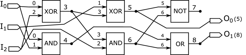
Figure 1: A full adder represented by CGP. Chromosome: (0, 2, 2) (0, 1, 0) (1, 3, 2) (3, 2, 0) (5, 6, 3) (4, 6, 1) (5, 8), node functions: AND (0), OR (1), XOR (2), NOT (3).

We use a standard CGP that employs the (1+$\lambda$) search method where a single generation of candidates consists of the parent and $\lambda$ offspring candidates. The fitness of each of the solutions is evaluated and the best solution is preserved as the parent for the next generation. Other candidates from the generation are discarded.

In circuit approximation, the evolution loop typically starts with a parent representing a correctly working circuit. New candidate circuits are obtained from the parent using a mutation operator which performs random changes in the candidate’s chromosome in order to obtain a new, possibly better candidate solution. The mutations can either modify the node interconnection or functionality. The number of the nodes of candidate circuits is reduced by making some nodes inactive, i.e. disconnected from the outputs of the circuit. However, since such nodes are not removed, they can still be mutated and eventually become active again.

The whole evolution loop is repeated until a termination criterion (in our case, a time limit fixed for the evolution process) is met. For more details of CGP, see [36].

4.2 Candidate circuit evaluation

Recall that the candidate circuit evaluation takes into consideration two attributes of the circuit, namely, whether the approximation error represented by WCAE is smaller than the given threshold and the size of the circuit. Formally, we define the fitness function $f$ in the following way:

$$f(C)=\begin{cases}\mathrm{size}(C)&\mbox{ if }\mbox{WCAE}(G,C)\leq\mathcal{T},\\ \infty&\mbox{ otherwise.}\end{cases}$$

The procedure deciding whether $\mbox{WCAE}(G,C)\leq\mathcal{T}$ represents the most time consuming part of the design loop. Therefore, we call the procedure only for those candidates $C$ that satisfy that ${\mathrm{size}(C)\leq\mathrm{size}(B)}$ where $B$ is the best solution with an acceptable error that we have found so far.

To decide whether $\mbox{WCAE}(G,C)\leq\mathcal{T}$, we adopt the concept of an approximation miter introduced in [14, 37]. The miter is an auxiliary circuit that consists of the inspected approximate circuit $C$ and the golden circuit $G$ which serves as the specification. $C$ and $G$ are connected to identical inputs. A subtractor and a comparator then check whether the error introduced by the approximation is greater than a given threshold $\mathcal{T}$. The high-level structure of the approximation miter is shown in Fig. 2. The output of the miter is a single bit which evaluates to logical 1 if and only if the constraint on the WCAE is violated for the given input $x$.

Once the miter is built, it is translated to a Boolean formula that is satisfiable if and only if ${\mbox{WCAE}(G,C)>\mathcal{T}}$. This approach allows one to reduce the decision problem to a SAT problem and use existing powerful SAT solvers. Of course, this is a high-level view only. On the gate-level, we optimize the miter construction by using a novel circuit implementation of the subtractor, absolute value, and comparator nodes as described in the conference paper [17]. The construction, whose details we skip here since they are rather hardware-oriented, leads to structurally less complex Boolean formulas. In particular, it avoids long XOR chains, which are a known cause of poor performance of the state-of-the-art SAT solvers [38]. For details see [17].

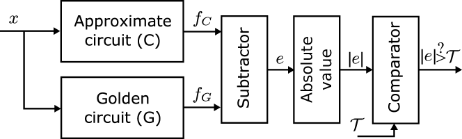
Figure 2: A high-level view on the typical approximation miter for the WCAE analysis, typically $e(x)=f_{G}(x)-f_{C}(x)$.

4.3 Verifiability-driven search

During our initial experiments with the approximation of large circuits, we discovered that the time required for the miter-based circuit evaluation can significantly differ even among structurally very similar candidates. For example, there are 16-bit approximate multipliers where checking that ${\mbox{WCAE}(G,C)\leq\mathcal{T}}$ holds takes less than a second, however, other similar approximations require several minutes. Additionally, we observed that the more complex the circuits to be approximated are, the higher are the chances that the evolution stumbles upon a solution that requires a prohibitive evaluation time. If such a candidate is accepted as a parent, its offspring are likely to feature the same or even longer evaluation time. Therefore, the whole evaluation process slows down and does not achieve any significant improvements in the time limit available for the entire optimisation.

To alleviate this problem, we propose a verifiability-driven search strategy that uses an additional criterion for the evaluation of the circuit $C$. The criterion reflects the ability of the decision procedure, in our case a SAT solver, to prove that ${\mbox{WCAE}(G,C)\leq\mathcal{T}}$ with a given limit $L$ on the resources available. It leverages the observation that a long sequence of candidate circuits $B_{i}$ improving the size and having an acceptable error has to be typically explored to obtain a solution that is sufficiently close to an optimal approximation $C^{*}$. Therefore, both the SAT and the UNSAT queries to the SAT solver have to be short. If the procedure fails to prove $\mbox{WCAE}(G,C)\leq\mathcal{T}$ within the limit $L$, we set $f(C)=\infty$ and generate a new candidate.

The interpretation of the resource limit $L$ on checking that $\mbox{WCAE}(G,C)\leq\mathcal{T}$ depends on the implementation of the underlying satisfiability checking procedure. Note that a time limit is not suitable since it does not reflect how the structural complexity of candidate circuits affects the performance of the procedure. Therefore, we employ the limit on the maximal number of backtracks in which a single variable can be involved during the backtracking process (also called the maximal number of conflicts on a variable). As the backtracking represents the key and computationally demanding part of modern SAT solvers [39], it allows one to effectively control the time needed for particular evaluation queries. Moreover, it takes into account the structural complexity of the underlying boolean formula capturing the complexity of the circuit.

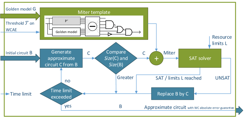
Figure 3: The main steps of the proposed verifiability-driven search scheme.

The overall optimisation loop using the verifiability-driven search is illustrated in Fig. 3. The inputs of the design process include: (1) the golden model $G$, (2) the threshold on the worst-case absolute error $\mathcal{T}$, (3) the initial circuit $B$ having an acceptable error (it can be either the golden model or its suitable approximation that we want to start with), and (4) the time limit on the overall design process. The loop exploits the CGP principles for the case of $\lambda=1$, i.e. for populations consisting of the parent and a single child, which turns out to be a suitable setting in our experiments discussed below. In other words, the loop uses mutations to generate a single new candidate circuit $C$ from the candidate circuit $B$ representing the best approximation of the circuit $C^{*}$ that we have found so far. The circuit $C$ is then evaluated using the fitness function $f$ as described above. If the candidate $C$ belongs to an improving sequence (i.e. ${\mathrm{size}(C)\leq\mathrm{size}(B)}$ and $\mbox{WCAE}(G,C)\leq\mathcal{T}$), we replace $B$ by $C$. The design loop terminates if the overall time limit is reached, and $B$ is returned as the output of the design process.

4.4 Adaptive resource limit strategy

In our original conference paper [17], we performed a preliminary experimental evaluation of the verifiability-driven search strategy studying how the limit $L$ on the maximal number of backtracks in the SAT decision procedure affects the performance of the approximation process applied on multipliers and adders of various bit-widths. In particular, we considered 20K, 160K, and unboundedly many backtracks. The results clearly demonstrated that the evolutionary algorithm found best solutions for the lowest of these three limit settings for a wide range of circuits. However, the question whether a still lower SAT limit would improve the performance even further remained open. Likewise, there remained a question what limits would be appropriate for other circuits than those considered in the experiments.

Apparently, the lower the limit is the faster the evaluation of each candidate solution will be. This results in processing a higher number of generations in a given time interval, hopefully leading to better results. On the other hand, aggressive limit settings reduce the search space of candidate solutions that can be evaluated within the given limit. A too tight restriction might prevent the candidate solutions from diverting from the original solution and reaching significant improvements (most of the newly generated candidates will likely be skipped due to exceeding the evaluation limit). Also, the type and complexity of the approximated circuit and the approximation error can play a significant role in choosing ideal limit settings. Thus, to reach the best performance of the method, each new instance of the problem would require an evaluation of different limit values. Moreover, a fixed limit value might not be optimal during the course of the evolutionary process even if it is optimal in some of its phases.

Therefore we propose a new adaptive strategy that alters the limit within the evolutionary run and tries to set it to the most suitable value with regards to the recently achieved progress. We designed the strategy scheme based on our previous observations that the limit should be kept low in the early stages of the evolution so that the clearly redundant logic can be quickly eliminated. Later in the evolutionary process, the algorithm converges to a locally optimal solution and improvements in the fitness cease to occur. When such a stage is reached, the limit needs to be increased in order to widen the space of feasible candidate solutions at the expense of slower candidate evaluation. Moreover, once some more significantly changed solution is found, it may again be possible to shorten the time limit needed for the evaluation, and the process of extending and shrinking the time limit may repeat (as witnessed also in our experiments).

Algorithm 1 Adapting the time limit for evaluating candidates

1:$lastGens\leftarrow 0$

2:$improvementCount\leftarrow 0$

3:function updateLimit(limit, improvement)

4:     $lastGens\leftarrow lastGens+1$

5:     if $improvement$ then

6:         $improvementCount\leftarrow improvementCount+1$      

7:     if $lastGens\text{ mod period}=0$ then

8:         if $improvementCount>\tau_{dec}$ then

9:              $limit\leftarrow limit-\delta*limit$

10:         else if $improvementCount<\tau_{inc}$ then

11:              $limit\leftarrow limit+\delta*limit$          

12:         $improvementCount\leftarrow 0$

13:         $lastGens\leftarrow 0$

14:     else if $improvementCount>\tau_{res}$ then

15:         $lastGens\leftarrow 0$

16:         $improvementCount\leftarrow 0$

17:         $limit\leftarrow limit-\delta*limit$      

18:     $limit\leftarrow max(limit,minLimit)$

19:     $limit\leftarrow min(limit,maxLimit)$

20:     return limit

Our strategy is described in pseudocode in Algorithm 1. The strategy changes the limit during the evolution process and is driven by four main parameters and two additional limit values with the following semantics:

• $period$: the number of generations after which a periodic check whether the evaluation limit should be changed is triggered.

• $\delta$: the increase/decrease ratio which says by what fraction of the current limit the limit is increased/decreased when such a change is considered useful.

• $\tau_{dec}$: if the number of improvements that occur in a period is above this threshold, the time limit for the evaluation will be decreased.

• $\tau_{inc}$: if the number of improvements that occur in a period is below this threshold, the time limit for the evaluation will be increased.

• $\tau_{res}$: if this threshold is hit, an immediate decrease of the time limit and a reset of the generation counter is triggered. This threshold applies when the limit becomes clearly too high, which can happen as witnessed by our experiments.

• $minLimit$: a minimum limit bound that restricts the possible values of the time limit achievable by the adaptive strategy from below.

• $maxLimit$: a maximum limit bound that restricts the possible values of the time limit achievable by the adaptive strategy from above.

Algorithm 1 allows the strategy to track the current progress of the evolutionary algorithm and adapt the resource limit accordingly. The key purpose of the algorithm is to keep the limit low while the evolutionary process achieves improvements in the candidate solutions and increase the available resources once the progress is seemingly stalled by the imposed limit. The control algorithm tracks the number of improvements made in the last $lastGen$ generations in a global variable $improvementCount$. If the number of current improvements exceeds the value of $\tau_{res}$, the limit is immediately decreased. Otherwise, the algorithm waits until the $period$ number of generations is reached and then either increases or decreases the limit based on the comparison of the $improvementCount$ and the thresholds $\tau_{inc}$ or $\tau_{dec}$, respectively.

The value of the increment/decrement of the resource limit is relative to the current limit value. This allows the strategy to both delicately alter small limit values and reach high limit values in reasonable time. The limit value is restricted to stay within the interval $\langle minLimit,maxLimit\rangle$. This ensures that we do not get too small limit values that would reject all candidates nor too big limit values that would feature a very long evaluation time, which would practically stop the approximation process.

5 Experimental Evaluation

In this section, we present a detailed experimental evaluation of the proposed method for evolutionary-driven circuit approximation. We first describe the experimental setting and briefly discuss the CGP parameters we used in the evaluation. Afterwards, we present a thorough evaluation of the adaptive feature of our approach as well as an overall comparison of our approach with other existing approaches. In particular, our experiments focus on answering the following research questions:

• Can the adaptive strategy reduce the randomness of the evolution-based approximation process?

• Can the adaptive strategy efficiently handle different circuit approximation problems – is it more versatile than the fixed-limit strategies?

• Can the adaptive strategy outperform the best fixed-limit strategy for a given circuit approximation problem?

• Does the proposed method significantly outperform other circuit approximation techniques?

5.1 Experimental setup

The proposed circuit approximation method was implemented in our tool called ADAC—Automatic Design of Approximate Circuits [18]. ADAC is implemented as a module of ABC [31], a state-of-the-art academic tool for hardware synthesis and verification. ABC provides means for exact equivalence checking but also general SAT solving. We use the latter for solving our approximation miters.

In the experiments, we consider the following circuits for evaluating the performance of the proposed method:

• 16-bit multipliers (the input is two 16-bit numbers) having 1525 gates (501 xors and logic depth 34),

• 24-bit multipliers having 3520 gates (1157 xors and logic depth 40),

• 24-bit multiply-and-accumulate (MAC) circuits (the input is two 12-bit numbers and one 24-bit number) having 1023 gates (321 xors and logic depth 39),

• 32-bit MAC circuits having 1788 gates (565 xors and logic depth 44),

• 20-bit squares (the input is one 20-bit number, the result is second power of the input) with 2213 gates (789 xors and logic depth 38),

• 28-bit squares with 4336 gates (1547 xors and depth 40).

• 23-bit dividers (the input is 23-bit and 12-bit numbers) having 1512 gates (253 xors and logic depth 455),

• 31-bit dividers with 2720 gates (465 xors and depth 799),

Recall that we consider the circuit size as the key non-functional characteristic we want to improve by allowing an error in the circuit computation. To estimate the circuit size, we use the gate sizes listed in Table 1. These sizes correspond to the 45nm technology which we consider in Section 5.7 when comparing the power-delay product of our resulting circuits with state-of-the-art solutions.

Table 1: Sizes of the gates used in the experiments. The sizes are in $\mu m^{2}$ and correspond to the 45nm technology.

Gate	INV	AND	OR	XOR	NAND	NOR	XNOR
Size	1.40	2.34	2.34	4.69	1.87	2.34	4.69

Justification for the selected benchmark set:

Approximation of 16-bit multipliers represents the cutting edge of circuit approximation techniques due to the circuit size (i.e. the number of gates) and structural complexity (i.e. the presence of carry chains), especially when some formal error guarantees are expected from the approximation method. We use such multipliers in Section 5.7 to compare our approach with state-of-the-art techniques. The other circuits we consider go beyond this edge: MACs have a more complicated structure and the error of the involved multiplication is further propagated in the consequent accumulation. Square circuits computing the second power of the input represent a specialised version of multipliers, while these circuits feature less inputs than other examined instances, their internal structure is much more complex than the structure of arithmetic circuits with comparable input bit widths. Approximation of dividers represents a true challenge since they are structurally more complicated, much deeper, and significantly less explored (e.g. when compared with multipliers).

For all 8 circuits, we consider various WCAE values, namely, we let WCAE range from $10^{-4}\%$ to $1\%$. The given bound on the WCAE value determines permissible changes in the circuit structure (i.e. a small error allows only smaller changes in the circuit). Therefore, different WCAE values lead to significantly different approximation problems. We also consider two time limits (1 and 6 hours) for the approximation process. Note that, the time limit also considerably affects the approximation strategy as the given time has to be effectively used with respect to the complexity of approximation problem

In our experimental evaluation, we explore all three dimensions characterising the circuit approximation problems: i) the circuit type reflecting both the size and the structural complexity, ii) the error bound, and iii) approximation time. In total, we examine more than 70 instances of the approximation problems that sufficiently cover practically relevant problems in the area of arithmetic circuits approximation. Therefore, the considered benchmark allow us to answer the research questions and, in particular, to robustly evaluate the versatility of the adaptive strategies and their benefits with respect to the fixed-limit strategies.

Note that we exclude adders from our experimental evaluation as they represent a much simpler approximation problem – comparing to 16-bit multipliers, 128-bit adders have only around 1/3 of the gates and are structurally less complex. Therefore, the miter-based candidate evaluation handle these circuits without leveraging the resource limits.

5.2 CGP parameters

The performance of CGP for particular application domains can be tuned by various CGP parameters out of which the following are relevant in our case:

• the number of offsprings ($\lambda$),

• the frequency of mutations, and

• the CGP grid size and the L-back parameter (i.e. connectivity in the chromosome).

We now briefly discuss our choice of the values of these parameters that will later be used for the main part of the evaluation of the proposed method.

The literature shows that, for a fixed number of generated and evaluated candidate solutions, CGP-based circuit optimization (i.e. when circuits are not evolved from scratch) with a smaller value of $\lambda$ usually leads to better fitness values than CGP using larger values of $\lambda$ [41].

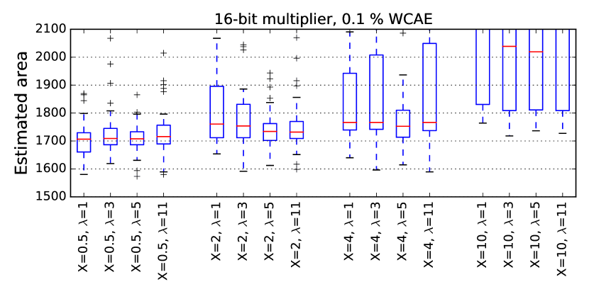
Figure 4: The impact of the number of offsprings ($\lambda$) and mutation frequency ($X$) on the final circuit area of approximated 16-bit multipliers obtained by CGP with a fixed time limit for each evolutionary run.

Aside from the population size, we also examine the effect of the mutation frequency on the performance of circuit approximation. Each time the mutation operator is applied, it alters a single integer in the chromosome. When we generate a new candidate from a parent, we apply the mutation operator up to $M$ times, $M=0.01*X*gates(G)$ where $X$ is the mutation frequency parameter and $gates(G)$ is the number of gates of the golden solution $G$ that is approximated. In our particular experiment, in which $gates(G)=1525$, the performance was evaluated for $X\in\langle 0.5,10\rangle$, i.e. $M\in\langle 8,153\rangle$ mutations per chromosome.

Fig. 4 provides the results of approximation of 16-bit multipliers with 0.1 % WCAE using different combinations of $\lambda$ and $X$ (the $x$-axis). The $y$-axis characterises the size (obtained as the sum of gate sizes) of the best candidate found in every $2$-hour run. The SAT resource limit was set to $100$. We do not present results for other approximate circuits as they exhibit similar patterns. The boxplots are grouped by mutation frequency. We can see that the performance within each group is very similar and lower mutation frequencies perform better than higher mutation frequencies. We also applied Friedman and Nemenyi statistical tests [42, 43, 44] to evaluate these results. According to Nemenyi post hoc test, the differences between various $\lambda$ values within the same mutation frequency are not significant at $\alpha=0.05$. Mutation frequencies $X=0.5$ and $X=2$ are equivalent and perform significantly better than $X=4$ and $X=10$.

Our experiments confirm general observations known from the literature (see, e.g., [4]): the number of mutations should be small. This way, the mutations perform slight changes between the generations only. Otherwise, for a high mutation frequency, the function of a new solution is usually completely altered. Such a solution is then rejected with a high probability, the search gets close to a random one, and its efficiency deteriorates. Therefore, in the rest of the experiments, we choose the mutation frequency $X=0.5~{}\%$. As population size does not seem to significantly matter, we choose the simplest $\lambda=1$ scheme.

Finally, we set the dimensions of the chromosome gate matrix as $1\times W$ where $W$ equals the number of gates in the correct circuit (i.e. all the gates of the original circuit are in one row) and use L-back = $W$, i.e. we allow the maximum connectivity of the chromosomes. This setting gives the evolutionary algorithm maximal freedom with respect to the candidate solutions that can be created. This fact is desirable in case of area optimization we aim at [35, 36].

5.3 Comparison of adaptive strategies

In the next phase of our experiments, we examine different versions of the adaptive strategy corresponding to different instantiations of the adaptive scheme presented in Section 4.4. The goal of this phase is to select the best adaptive strategies that efficiently works for a wide class of approximation problems. These strategies are further thoroughly evaluated and compared with fix-limit strategies on the selected benchmark.

Based on our experience with the limit values used in [17], we consider five versions of the adaptive strategy given by the parameter values listed in Table 2. These versions have been chosen to adequately cover the space of adaptive strategies and thus they range from strategies that try to promptly react to changes in the evolutionary process ($ada1$, $ada3$) to strategies that evaluate the progress of the evolution over longer periods of time ($ada2$). The remaining strategies ($ada4$, $ada5$) lie in the middle of the range.

The strategies differ mainly in two basic aspects: the length of the period with which the adaption happens and the thresholds used for the adaption ($\tau_{dec}$, $\tau_{inc}$, $\tau_{res}$). Larger values of the thresholds with respect to the $period$ mean that the resource limit will more likely be increased. Strategies with such thresholds ($ada1$, $ada3$ and $ada5$) are faster to magnify the limit once the evolution seemingly gets stuck in a local optimum. Thus, the possible search space is broadened, but each candidate evaluation is likely to take longer time. On the other hand, strategies $ada2$ and $ada4$ try to keep the resource limit as low as possible, and each evaluation is therefore very fast. However, once there are no improvements possible with the current limit value, these strategies are slower to react.

The minimal limit value $minLimit$ and the maximum limit value $maxLimit$ are set to 500 and 15,000, respectively, based on the experience we gained from our previous work [17].

Table 2: Adaptive strategy parameters.

Strategy	$\tau_{dec}$	$\tau_{inc}$	$\tau_{res}$	period	minLimit	maxLimit
ada1	4	2	10	1000	500	15000
ada2	2	1	5	15000	500	15000
ada3	4	4	8	3000	500	15000
ada4	1	1	3	5000	500	15000
ada5	5	4	8	5000	500	15000

We evaluate the performance of the described strategies on the approximation scenario of 16-bit multipliers with a total of 8 target WCAE values ranging from $10^{-4}\%$ to $1\%$ with 50 independent 1 hour and 6 hour long evolutionary runs. The quality of the obtained final solutions was evaluated using Friedman and Nemenyi statistical tests with results illustrated in Table 3.

For 1h runs, stategy $ada5$ performs the best, but it’s performance is statistically equivalent to $ada4$ and $ada3$. This group of strategies is significantly better than $ada1$ and $ada2$.

For 6h runs, $ada2$ significantly outperforms the rest of strategies, followed by $ada4$ which also significantly outperforms its successors.

In the overall evaluation, the group $ada2$, $ada4$ and $ada5$ is statistically equivalent and significantly better than strategies $ada1$ and $ada3$. As we aim to acquire the best solutions that our method can provide, we select the strategies $ada2$ and $ada4$ as representatives of adaptive strategies for the following experiments.

Table 3: Pairwise p-values of Nemenyi statistical test and average rank values for 1h experiments, 6h experiments and combined.

1h runs	$ada1$	$ada2$	$ada3$	$ada4$	$ada5$
$ada2$	0.74708	-	-	-	-
$ada3$	6.50E-06	0.00155	-	-	-
$ada4$	4.30E-07	0.00019	0.98709	-	-
$ada5$	9.20E-13	4.10E-09	0.09467	0.27627	-
Rank	3.4275	3.2925	2.87125	2.815	2.59375
6h runs	$ada1$	$ada2$	$ada3$	$ada4$	$ada5$
$ada2$	2.00E-16	-	-	-	-
$ada3$	0.28188	4.90E-14	-	-	-
$ada4$	5.40E-14	0.01082	3.10E-12	-	-
$ada5$	0.00013	6.50E-14	0.12034	9.10E-06	-
Rank	3.6275	2.23125	3.4075	2.5925	3.14125
Overall	$ada1$	$ada2$	$ada3$	$ada4$	$ada5$
$ada2$	6.10E-14	-	-	-	-
$ada3$	9.00E-06	1.80E-05	-	-	-
$ada4$	5.20E-14	0.9483	3.60E-07	-	-
$ada5$	5.30E-14	0.6686	0.0053	0.2326	-
Rank	3.5275	2.761875	3.139375	2.70375	2.8675

We further show how the adaptive strategies $ada2$ and $ada4$ change the resource limits during the approximation process. Fig. 5 shows how the limits change (increase as well as decrease) over the time during the approximation of the 16-bit multipliers with target $0.1\,\%$ WCAE. The approximation ran for 6 hours, and the plot shows the maximum number of SAT backtracks (i.e. the resource limit) that was allowed to be used during the verification of candidate circuits in particular generations of the evolution optimisation. The top two plots of the figure illustrate five selected runs for both strategies, and the bottom plot shows the aggregated results for 50 independent runs. It shows the median of the resource limits plotted by the full lines and quartiles Q1 and Q3 plotted by the dashed lines.

The figure confirms our expectations: in the initial stages of the approximation, the limit is kept low because improvements are found frequently. We can also see that the limit increases as well as decreases, and a closer evaluation of our data reveals that both the periodic and immediate decrease are used. Further, note that $ada4$ increases the limit much sooner than $ada2$, and the rate of the increase is also much steeper. This fact allows $ada4$ to use more time out of the total time available for the entire evolutionary run for evolving and evaluating solutions that need larger resource limits for their verification. On the other hand, the higher limit slows the evolutionary process down significantly—we see that none of the $ada4$ runs reaches the number of $1.2*10^{6}$ generations in this experiment. The particular runs of the strategies also demonstrate that $ada4$ exhibits more changes (including periodic drops of the limits) compared with the more stable strategy $ada2$. The impact of these differences on the quality of the obtained final solutions will be evaluated in the further subsections of this section.

Finally, Fig. 6 shows the aggregated results for approximation of 23-bit dividers (with the same WCAE) representing a very different approximation scenario. We observe that the approximation of the dividers requires higher resource limits (i.e. more time for the verification of the candidate solutions) when compared with the multipliers: this is due to the structural complexity of the circuits. For example, in the 400K-th generation, $ada2$ sets the limit to about 2K for the multipliers and to about 12K for the dividers. Note that the difference is, however, less significant in the case of $ada4$.

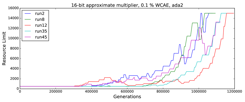
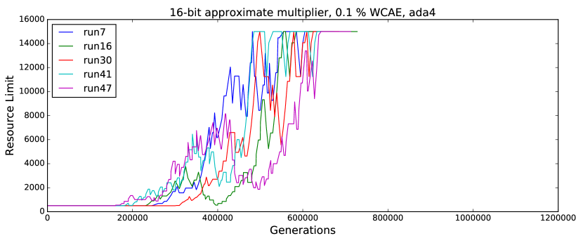
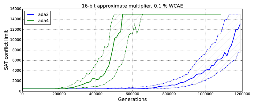
Figure 5: The resource limits chosen by the adaptive strategies $ada2$ and $ada4$ during the approximation of the 16-bit multiplier. The top two plots illustrate five selected runs. The bottom plot shows the medians (full lines) and the quartiles Q1 and Q3 (dotted lines) over 50 runs.

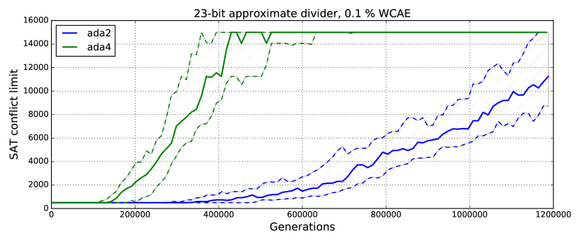
Figure 6: The resource limits chosen by the adaptive strategies $ada2$ and $ada4$ during the approximation of a 23-bit divider. The plot shows the median values (full lines) and the quartiles Q1 and Q3 (dotted lines) over 50 runs.

5.4 Reduction of randomness (Q1)

Evolutionary algorithms involve a significant amount of randomness, and the quality of the final solutions produced by independent runs can considerably vary. One of the goals of the newly designed adaptive strategies is to reduce the amount of the involved randomness and ensure that most of the approximation runs will lead to high-quality solutions. In this part of experiments, we examine the quality and variability of sets of 50 independent evolutionary runs for the adaptive strategies as well as for various fix-limit resource settings.

In the following experiments, we denote the fixed resource limit strategies as $lim100$, $lim2K$, $lim10K$, $lim20K$, and $lim50K$ for the resource limits of $100$, $2000$, $10000$, $20000$, and $50000$ backtracks on a single variable, which are used through the whole evolutionary process. We chose these values to represent small, mid range, and large values. In our previous work [17], we used $lim20K$ as the standard resource limit setting.

The plots in Fig. 7 demonstrate how the size of the candidate solutions decreases during particular runs. In particular, the dashed red lines show the best and the worst run; and median, first (Q1) and third (Q3) quartile are illustrated by the full blue line and the red lines, respectively.

The figure shows that the adaptive strategies as well as the strategies with lower resource limit values are significantly more stable than the strategies with higher limits. This is caused by the fact that the evolution has to explore solutions requiring a long verification time. Such solutions are immediately refused by the lower resource limits ($100$, $2K$) and by the adaptive strategies but more likely accepted by the other strategies ($10K$, $20K$, and $50K$). The long evaluation time is inherited from parents to offsprings. The strategies with higher limit settings are therefore much slower to converge to a near optimum solution. The previously described slowdown of the evolution also leads to higher variation in the candidate quality throughout the evolution, which can be observed as the wide interquartile range (IQR) for limits $10K$, $20K$, and $50K$. Other strategies feature a narrow IQR—a desirable attribute of a good resource limit strategy. The convergence of the strategy $lim50K$ is so slow that we exclude this strategy from the rest of the experiments to save computational time.

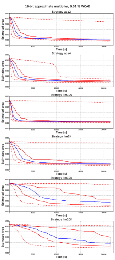
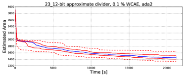
Figure 7: Convergence curves for resource limit strategies showing the estimated area for the best, worst, Q1, Q3, and median solutions during 16-bit multiplier and 23-bit divider approximation.

We obtained similar observations for other WCAE values and bit-width settings for multipliers, MACs and square circuits. The difference between strategies is even more pronounced for smaller approximation errors, which represent a harder optimization problem. On the other hand, large approximation errors diminish the differences.

The approximation of dividers represents another class of optimization problems with a different behaviour. The variance of the solutions is very similar for all resource limit settings. This fact is illustrated in the bottom part of Fig. 7. While the variance is almost identical, what differs between the resource limit strategies is the quality of final solutions that can be achieved. This is described in greater detail in the next section.

Summary for Q1: For a wide class of circuits, the adaptive strategies as well as the low-limit strategies are significantly more stable than other fixed limit strategies (i.e. the effect of the randomness is smaller). All strategies show good stability for the approximation of dividers, however, the low-limit strategies provide considerably smaller reductions of the circuit area.

Note: Since it would be very difficult to present our results while also showing the randomness of the evolutionary runs at the same time, we present only the quality of the median solutions in the rest of our paper when not stated otherwise.

5.5 Versatility of adaptive strategies (Q2)

The key feature of circuit approximation strategies is versatility, an ability to provide excellent performance for various approximation scenarios including different circuits, WCAE values, and time limits. Although the verifiability-driven strategy itself leads to unprecedented performance and scalability of circuit approximation [17], the fixed-limit resource limits do not ensure versatility. This fact is demonstrated in Fig. 8 where we fix WCAE to $0.1~{}\%$ for multipliers, squares, MACs, and dividers, and explore the progress of the approximation process. The right part of each plot illustrates the quality of the final solutions.

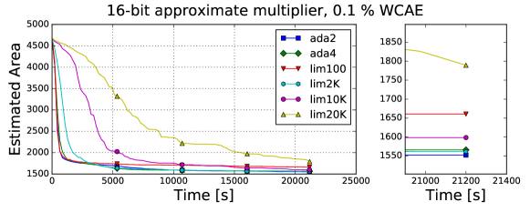
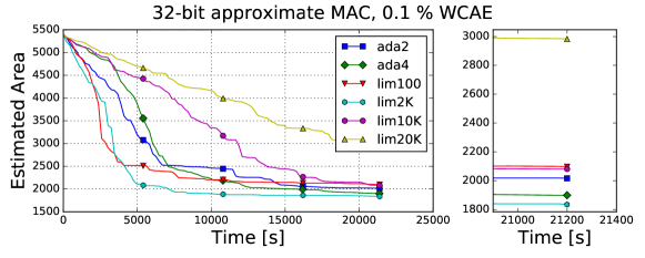
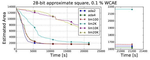
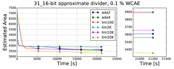
Figure 8: Convergence plots of median solutions calculated from 50 independent evolutionary runs for various combinational circuits.

When comparing the performance of the fixed-limit strategies on the approximation of 16-bit multipliers, we can see that the strategy $lim100$ dominates in the first hour of the approximation process since it provides the fastest convergence. Strategies $ada2$, $ada4$, and $lim2K$ converge slower, but around after the first hour their median solutions outperform $lim100$ which cannot achieve further improvements due to the tight resource limit. Strategies $lim10K$ and $lim20K$ provide a significantly slower converge: $lim10K$ needs around 2.5 hours to provide solutions that are comparable to the aforementioned strategies, $lim20K$ is too slow and its final solution lags behind.

Similar trends among the inspected strategies are observed for the 32-bit MACs (see the second plot in Fig. 8). Note that, in general, the convergence is much slower because this circuit is larger and represents a harder optimization problem compared with the multipliers. Moreover, we observe a larger diversity among the strategies.

The progress tendencies for 28-bit square circuit (see the third plot in Fig. 8) significantly differ. The strategies $lim10K$ and $lim20K$ provide an extremely slow converge and even after 6-hours runs they significantly lag behind the other strategies. The strategies $lim2K$ also converges much slower than the remaining strategies, which show similar performance. After an 1-hour run, $lim2K$ returns circuits that are about two-times larger than the circuits provided by the strategy $lim100$, however, after 5 hours it catches up with the other strategies.

The bottom part of Fig. 8 illustrates results for the dividers. We observe a very different trend in the approximation process. In particular, all strategies converge very quickly to a sub-optimal solution, but the fixed-limit strategies with small resource limits ($lim100$ and $lim2K$) are not able to achieve any further improvement, and they significantly lag behind other strategies in the final solutions. We further observe that the strategy $lim20K$, which performes very poorly on the previous circuits, is the best strategy in this case. The proposed adaptive strategies inherit the initial fast convergence using a small limit, but they adapt the limit after the first hour and arrive to results comparable with the strategy $lim10K$.

Fig. 8 indicates that the performance of the particular fixed-limit strategies fundamentally varies for different circuits under approximation. For example, the strategy $lim2K$ gives the best results for the MACs, but it behaves very poorly on the dividers, which clearly require a very high resource limit. In Tables 4–6, depicting the results for particular circuits, we show that the selection of the best strategy also depends on the required WCAE and on the bit-width of the particular circuits. The tables list the relative size reductions of the median solutions with respect to the golden circuit obtained using different strategies after 1 and 6 hours for different circuit types, bit-widths, WCAEs. The best solution for each target approximation error is highlighted in bold text. For instance, Table 4 shows that the median solution for 16-bit multipliers with $0.01~{}\%$ WCAE obtained by $ada4$ in 6 hours has the area of $54~{}\%$ of the original 16-bit multiplier. The quality of this solution dominates the solutions obtained by other strategies for this experimental setup.

Table 4: The relative sizes in % of median solutions with respect to the size of the golden solution for multiplier approximation.

16-bit multiplier
1h runs	$lim100$	$lim2K$	$lim10K$	$lim20K$	$ada2$	$ada4$
0.001 %	82.2	85.8	95.7	98.1	82.4	81.1
0.01 %	61.1	60.4	88.6	96.7	59.3	57.9
0.1 %	37.7	37.0	58.9	86.2	36.8	36.7
1 %	18.8	17.9	20.2	43.5	18.6	17.7
6h runs	$lim100$	$lim2K$	$lim10K$	$lim20K$	$ada2$	$ada4$
0.001 %	74.0	72.8	77.6	82.4	72.5	71.5
0.01 %	56.4	55.4	56.8	63.2	55.0	54.0
0.1 %	35.5	33.4	34.6	38.5	33.2	33.5
1 %	17.4	15.7	16.4	17.2	15.7	15.9

24-bit multiplier
1h runs	$lim100$	$lim2K$	$lim10K$	$lim20K$	$ada2$	$ada4$
0.001 %	91.2	87.6	96.7	97.7	89.0	87.2
0.01 %	32.1	59.7	89.3	94.4	32.8	31.5
0.1 %	19.0	19.8	78.7	86.3	18.4	18.5
1 %	9.2	8.6	21.1	79.9	9.1	8.9
6h runs	$lim100$	$lim2K$	$lim10K$	$lim20K$	$ada2$	$ada4$
0.001 %	43.0	40.4	79.3	82.6	41.8	41.0
0.01 %	27.1	27.1	30.2	42.7	26.8	26.3
0.1 %	16.3	15.9	18.1	23.4	15.9	16.0
1 %	8.7	7.6	7.6	8.6	7.4	7.4

Table 5: The relative sizes in % of median solutions with respect to the size of the golden solution for MAC approximation and divider approximation.

24-bit MAC
1h runs	$lim100$	$lim2K$	$lim10K$	$lim20K$	$ada2$	$ada4$
0.0001 %	96.7	96.9	97.7	97.8	96.7	97.1
0.001 %	94.3	93.7	95.0	95.3	94.0	93.9
0.01 %	91.3	82.1	83.0	95.5	90.0	93.9
0.1 %	73.1	67.8	93.2	92.6	65.8	64.1
1 %	38.2	28.9	45.4	67.9	31.1	28.5
6h runs	$lim100$	$lim2K$	$lim10K$	$lim20K$	$ada2$	$ada4$
0.0001 %	95.9	96.2	95.8	96.2	95.5	95.8
0.001 %	92.3	90.4	89.4	89.4	88.7	88.5
0.01 %	84.9	76.0	75.0	78.7	76.6	75.2
0.1 %	59.1	56.7	61.2	65.6	53.1	53.0
1 %	31.8	27.3	26.1	26.9	24.7	24.9

32-bit MAC
1h runs	$lim100$	$lim2K$	$lim10K$	$lim20K$	$ada2$	$ada4$
0.0001 %	94.6	95.7	98.7	98.9	95.0	94.8
0.001 %	94.3	94.0	97.5	97.6	93.8	93.6
0.01 %	87.1	81.2	90.0	95.5	85.5	89.3
0.1 %	87.1	57.8	85.7	90.8	77.3	86.2
1 %	24.8	19.1	32.0	58.3	19.4	19.7
6h runs	$lim100$	$lim2K$	$lim10K$	$lim20K$	$ada2$	$ada4$
0.0001 %	93.7	88.9	93.7	94.3	91.2	88.0
0.001 %	91.9	78.0	83.4	80.8	80.5	76.9
0.01 %	61.1	60.4	55.6	62.5	57.9	62.7
0.1 %	39.7	34.0	39.1	54.8	37.4	35.1
1 %	20.3	17.1	16.4	16.4	15.5	15.3

23-bit divider
1h runs	$lim100$	$lim2K$	$lim10K$	$lim20K$	$ada2$	$ada4$
0.05 %	76.8	76.6	76.4	74.2	76.7	76.6
0.1 %	72.7	71.1	66.7	65.1	71.3	68.4
0.5 %	51.4	48.2	43.1	43.4	48.9	46.0
1 %	42.3	37.2	33.2	34.6	39.8	35.7
6h runs	$lim100$	$lim2K$	$lim10K$	$lim20K$	$ada2$	$ada4$
0.05 %	73.7	74.3	72.4	69.9	72.6	72.5
0.1 %	66.5	67.8	63.9	61.4	62.7	62.8
0.5 %	47.8	44.0	38.6	39.9	40.1	39.8
1 %	39.0	32.2	29.4	30.2	30.3	31.0

31-bit divider
1h runs	$lim100$	$lim2K$	$lim10K$	$lim20K$	$ada2$	$ada4$
0.05 %	62.4	62.5	63.1	60.5	62.3	62.3
0.1 %	55.8	56.0	53.3	51.1	55.8	55.2
0.5 %	42.5	38.4	31.6	29.8	38.3	36.8
1 %	33.9	28.3	21.6	22.6	31.5	29.7
6h runs	$lim100$	$lim2K$	$lim10K$	$lim20K$	$ada2$	$ada4$
0.05 %	61.8	62.0	60.5	58.2	59.1	59.0
0.1 %	55.1	55.2	51.8	47.5	51.2	50.4
0.5 %	37.9	37.2	27.8	26.9	30.6	28.2
1 %	30.4	26.0	19.1	19.0	22.0	20.3

Table 6: The relative sizes in % of median solutions with respect to the size of the golden solution for square approximation.

20-bit square
1h runs	$lim100$	$lim2K$	$lim10K$	$lim20K$	$ada2$	$ada4$
0.0001 %	92.7	97.6	98.8	99.3	94.6	93.4
0.001 %	81.8	93.4	98.5	98.9	85.7	80.6
0.01 %	40.2	82.6	95.7	97.8	71.4	51.2
0.1 %	29.4	25.4	90.3	89.2	25.7	26.9
1 %	13.4	10.5	9.3	9.0	13.1	12.2
6h runs	$lim100$	$lim2K$	$lim10K$	$lim20K$	$ada2$	$ada4$
0.0001 %	70.1	82.9	92.2	97.6	70.5	68.8
0.001 %	54.6	61.2	94.5	96.0	55.1	54.3
0.01 %	38.6	37.4	51.1	81.4	38.0	36.3
0.1 %	22.8	22.6	31.4	21.9	21.9	21.1
1 %	12.2	7.9	7.1	7.2	7.7	7.3

28-bit square
1h runs	$lim100$	$lim2K$	$lim10K$	$lim20K$	$ada2$	$ada4$
0.0001 %	95.0	97.0	98.4	98.6	95.8	96.2
0.001 %	90.4	91.0	96.6	97.9	90.3	92.3
0.01 %	50.6	81.2	96.4	97.2	60.2	62.6
0.1 %	30.2	67.2	95.1	95.8	19.0	30.1
1 %	9.0	16.3	9.1	6.6	9.9	8.6
6h runs	$lim100$	$lim2K$	$lim10K$	$lim20K$	$ada2$	$ada4$
0.0001 %	56.1	77.1	93.0	96.8	67.5	70.4
0.001 %	31.4	40.1	81.0	87.9	32.0	32.3
0.01 %	20.6	22.7	73.9	86.4	21.0	20.5
0.1 %	12.3	16.0	57.9	43.3	12.2	12.0
1 %	6.5	4.6	4.1	4.0	4.8	4.2

Table 7: The overall versatility scores for the considered strategies aggregated over the bit-widths for each of the circuits.

	Multiplier		Divider		MAC		Square
time limit	1h	6h	1h	6h	1h	6h	1h	6h	AVG
$lim100$	104.1	106.9	121.7	124.1	109.8	114.4	116.3	115.4	114.1
$lim2K$	113.7	101.3	113.6	117.2	102.2	104.5	160.9	117.7	116.4
$lim10K$	201.7	118.8	102.6	103.0	126.3	106.0	196.7	206.6	145.2
$lim20K$	322.2	136.0	101.2	100.8	151.1	113.2	193.5	208.2	165.8
$ada2$	102.5	101.1	116.6	106.4	108.0	102.6	120.2	106.6	108.0
$ada4$	100.6	100.5	111.9	104.2	108.8	101.7	118.7	103.6	106.3

In order to effectively evaluate the overall performance and versatility of the different strategies, we introduce a versatility score. For each experimental setting, we set the versatility score of the strategy $B$ that found the best solution to $100~{}\%$, and other strategies $S$ are assigned the score of $area(S)/area(B)*100~{}\%$. In other words, this measure shows how many per cent larger the solution obtained by the chosen strategy is with respect to the best solution for the experiment (i.e., a lower score is better). As before, we compute the score from the median solutions produced by 50 independent evolutionary runs.

Table 7 shows the versatility scores of the inspected strategies computed for particular circuits considering 1 and 6 hours runs. These scores aggregate the results presented in Tables 4–6 and give us a better comparison among the strategies. The right-most column of Table 7 contains the versatility scores aggregated over all experiments. These scores allow us to answer the research question $Q2$, namely, we can compare the versatility of the fix limit strategies and the selected adaptive strategies.

The best versatility is achieved by the adaptive strategy $ada4$. The score $106.3$ shows that a median solution produced by this strategy is on average about $8$ percentage points worse than a median solution produced by the best strategy for a given experimental scenario. Strategy $ada4$ is closely followed by $ada2$ which is by roughly $2$ percentage points worse. The best performance from fixed-limit strategies is provided by $lim100$ that has the versatility score of $114.1$.

However, since the final values are computed as averages, the final ranking is skewed by $lim2K$’s poor performance for some problem instances in square circuit approximation (see Table 6: 1h runs for $0.01\%$ WCAE). If we excluded these experiments from the final evaluation, $lim2K$ would perform considerably better than $lim100$.

Table 8: The pair-wise p-values obtained using Nemenyi post-hoc test evaluated over all strategies and conducted experiments.

	lim100	lim2K	lim10K	lim20K	ada2
lim2K	0.39256	-	-	-	-
lim10K	0.99828	0.66932	-	-	-
lim20K	0.87598	0.02957	0.64037	-	-
ada2	0.00045	0.21525	0.00252	1.90E-06	-
ada4	8.00E-08	0.00124	9.30E-07	5.50E-11	0.55151

Figure 9: The pair-wise comparison of all strategies obtained by Nemenyi test. Groups of strategies that are not significantly different (at $\texttt{p-value}=0.05$) are connected.

We further perform Friedman statistical test with Nemenyi post hoc analysis to assess the significance of the results we obtained. In particular, we analyse the statistical significance of the versatility scores for particular approximation strategies across all conducted experiments. Friedman test returns $\texttt{chi-squared}=71.39$ and $\texttt{p-value}<5.2\mbox{E-14}$. These values clearly demonstrate that the versatility scores for particular strategies are not statistically equivalent. Therefore, we use Nemenyi post hoc analysis to identify the groups of statistically equivalent strategies. Table 8 shows the pair-wise $p$-values for all strategy pairs. Note that these values take into consideration the evaluation over all strategies and conducted experiments. Figure 9 illustrates the average ranks (with respect to the versatility scores) of examined strategies and also visualises the groups that are not significantly different at $\alpha=0.05$ We can conclude that strategy $ada4$ is highly significantly better ($\texttt{p-value}<0.01$) than all examined fixed limit strategies.

The statistical methods are rank based and thus they do not suffer from excessive sensibility to a few experiments with major differences in performance. Interestingly, the final placings in Fig. 9 (rank based) and Table 7 (average based) are identical with the exception of $lim100$. $Lim100$ provides decent solutions for each problem instance, hence scores well in the average based versatility score. On the other hand, it is slightly outperformed in each case by other strategies and so it’s rank is even worse than that of $lim10K$. Except for a few experiment instances, $lim2K$ places among the top strategies and comes third in the rank based rankings.

Summary for Q2: The adaptive strategies, in contrast to the fixed-limit strategies, are able to provide very good performance for a wide class of approximation problems. This is demonstrated by the highest versatility score as well as by the statistical significance tests.

5.6 A comparison of adaptive and fixed-limit strategies (Q3)

We saw that the adaptive strategies provide the best versatility score as well as rank score which indicates that they can effectively handle various approximation scenarios. In this section, we look closer at the results presented in Tables 4–6 and focus on interesting data points revealing weak and strong properties of the adaptive strategies. In particular, we will discuss if a single adaptive strategy can outperform the best fixed-limit strategy for a given circuit approximation problem.

Table 4 shows that the adaptive strategies dominate in almost all approximation scenarios for multipliers. In two scenarios, the strategy $lim2K$ slightly outperforms the adaptive strategies, however, it significantly lags behind for 1 hour runs and selected WCAEs (i.e. 24-bit version and $0.001~{}\%$ WCAE).

On the other hand, the adaptive strategies lack behind the best strategies mainly in two sets of experiments: MACs in 1 hour evolution and dividers in 1 hour evolution (see Tables 5). Their performance is similar to that of $lim100$, and they are outperformed by strategies with higher limit values. Since the adaptive strategies are designed to keep the limit as low as possible while still achieving some improvements in the candidate solutions, they do not increase their limit value during the first hour of the experimental evaluation. Our experiments show that even with a low resource limit, the strategies find improvements, but many of the candidate solutions are rejected because they cannot be evaluated within the limit. The difference in performance is diminished as the optimisation process continues and the adaptive strategies increase their resource limit. After 6 hours, the adaptive strategies outperform other settings for MACs and come close to the performance of $lim10K$ and $lim20K$ for dividers.

In case of square approximation, the adaptive strategies always produce a solution that is either the best or close to the best solution found. The exceptions are 1-hour runs for $0.01\%$ WCAE, and 6-hour run for 28-bit version and $0.0001\%$ WCAE, where $lim100$ significantly outperforms the other strategies.

Summary for Q3: The adaptive strategies provides the best performance (or are very close) for a wide class of approximation problems except for MACs with the short approximation time where low-limit strategies are slightly better due to faster convergence, and for dividers where high-limit strategies are better, due to the initial phase of the adaptive strategies.

5.7 A comparison with state-of-the-art techniques (Q4)

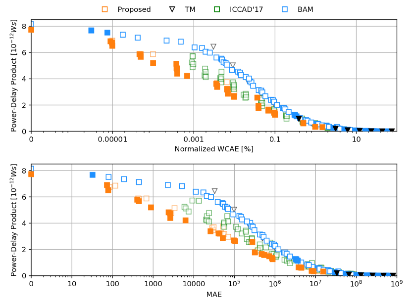
Figure 10: A comparison of 16-bit approximate multipliers obtained using the proposed approach and state-of-the-art approximation techniques. The plots show Pareto optimal solutions and their trade-offs between the precision and the power-delay-product (PDP)—the top plot depicts WCAE while the bottom plot depicts the mean absolute error (MAE). The filled marks represent solutions providing the best PDP for the given precision.

In this section, we demonstrate that our adaptive approach generates approximate circuits that significantly outperform circuits obtained using state-of-the-art approximation techniques. In particular, we show that our circuits provide significantly better trade-offs between the precision and energy consumption. We focus on multipliers since their approximation represents a challenging and widely studied problem—see, e.g., the comparative study of [27]. On the other hand, the existing literature does not offer a sufficient number of high-quality approximate MACs or dividers to carry out a fair comparison: indeed, our work is the first one that automatically handles such circuits.

In the comparison, we consider two approximate architectures for multipliers that are known to provide the best results, namely truncated multipliers (TMs) that ignore the values of least significant bits and broken-array multipliers (BAMs) [45]. TMs and BAMs can be parameterised to produce approximate circuits for the given bit-width and the required error. In contrast to our search-based approach, these circuits are constructed using a simple deterministic procedure based on simplifying accurate multipliers. However, the method is applicable for design of approximate multipliers only. To demonstrate the practical impact of the proposed adaptive strategy, we also consider circuits presented in [17] obtained using verifiability-driven approximation with a fixed limit strategy — this is a prominent representative of the search-based strategies.

Fig. 10 shows the parameters of resulting circuits belonging to Pareto front. For each circuit, the figure illustrates the trade-off between the precision and the power-delay-product (PDP) that adequately captures both the circuit’s energy consumption and its delay. The top plot of the figure illustrates the WCAE–PDP trade-offs. We also evaluated the mean absolute error (MAE) [37] of the solutions since MAE represents another important circuit error metric. The results are presented in the bottom plot of the figure.

The orange boxes represent circuits obtained using the adaptive strategy $ada4$. The green boxes represent circuits presented in [17] and obtained using the fixed limit strategy $lim20K$. In both cases, the circuits were generated as follows: we selected 15 target values of WCAE (10 values for the strategy $lim20K$) and for each of these values, we executed 50 independent 2-hour runs using $\lambda=1$ and the mutation frequency $0.5\,\%$. The 10 best solutions for each WCAE were selected and synthesised to the target technology. Note that the strategy $lim20K$ provides a much smaller reduction of the chip area when very small values of WCAE are required and thus these small target values were not reported in [17].

As we have already shown in [17], the fixed-limit verifiability-driven approach leveraging SAT-based circuit evaluation is able to significantly outperform both TMs and BAMs and represents state-of-the-art approximation method for arithmetic circuits. Still, Fig. 10 shows that the proposed adaptive strategy improves our previously obtained results even further—given the same time limit, it generates circuits having significantly better characteristics.

Summary for Q4: The proposed approach combining the SAT-based candidate evaluation with the adaptive verifiability-driven search strategy provides a fundamental improvement of the performance and versatility over existing circuit approximation techniques.

6 Conclusion

Automated design of approximate circuits with formal error guarantees is a landmark of provably-correct construction of energy-efficient systems. We present a new approach to this problem that uniquely integrates evolutionary circuit optimisation and SAT-based verification techniques via a novel adaptive verifiability-driven search strategy. By being able to construct high-quality Pareto sets of circuits including complex multipliers, MACs, and dividers, our method shows unprecedented scalability and versatility, and paves the way for design automation of complex approximate circuits.

In the future, we plan to extend our approach towards different error metrics and further classes of approximate circuits. We will also integrate the constructed circuits into real-world energy-aware systems to demonstrate practical impacts of our work.

Acknowledgments: This work was partially supported by the IT4IXS: IT4Innovations Excellence in Science project (LQ1602) and the Brno PhD. Talent scholarship program.

References

- [1] Z. Vasicek, V. Mrazek, Trading between quality and non-functional properties of median filter in embedded systems, Genetic Programming and Evolvable Machines 18 (1) (2017) 45–82.
- [2] Z. Vasicek, et al., Towards low power approximate DCT architecture for HEVC standard, in: Proceedings of the Conference on Design, Automation and Test in Europe, DATE ’17, 2017.
- [3] H. R. Mahdiani, et al., Bio-inspired imprecise computational blocks for efficient vlsi implementation of soft-computing applications, TCAS-I (2010) 850 – 862.
- [4] V. Mrazek, et al., Design of power-efficient approximate multipliers for approximate artificial neural networks, in: Proc. of ICCAD’16, ACM, 2016, pp. 811–817. doi:10.1145/2966986.2967021.
- [5] Z. Vasicek, L. Sekanina, Evolutionary approach to approximate digital circuits design, IEEE Transactions on Evolutionary Computation 19 (3) (2015) 432–444. doi:10.1109/TEVC.2014.2336175.
- [6] K. Nepal, S. Hashemi, H. Tann, R. I. Bahar, S. Reda, Automated high-level generation of low-power approximate computing circuits, IEEE Transactions on Emerging Topics in Computingdoi:10.1109/TETC.2016.2598283.
- [7] V. Mrazek, R. Hrbacek, et al., Evoapprox8b: Library of approximate adders and multipliers for circuit design and benchmarking of approximation methods, in: Proc. of DATE’17, 2017, pp. 258–261.
- [8] A. Lotfi, A. Rahimi, et al., Grater: An approximation workflow for exploiting data-level parallelism in FPGA acceleration, in: 2016 Design, Automation Test in Europe Conf. Exhibition, DATE ’16, EDA Consortium, 2016, pp. 1279–1284.
- [9] C. Yu, M. Ciesielski, Analyzing imprecise adders using BDDs – a case study, in: Proc. of ISVLSI’16, IEEE, 2016, pp. 152–157.
- [10] A. Chandrasekharan, M. Soeken, D. Große, R. Drechsler, Approximation-aware rewriting of aigs for error tolerant applications, in: Proc. of ICCAD’16, IEEE, 2016, pp. 1 – 8.
- [11] Z. Vasicek, L. Sekanina, Formal verification of candidate solutions for post-synthesis evolutionary optimization in evolvable hardware, Genetic Programming and Evolvable Machines 12 (3) (2011) 305–327.
- [12] M. Ciesielski, et al., Verification of gate-level arithmetic circuits by function extraction, in: Proc. of DAC ’15, ACM, 2015.
- [13] A. Sayed-Ahmed, D. Große, et al., Formal verification of integer multipliers by combining Gröbner basis with logic reduction, in: Proc. of DATE’16, IEEE, 2016, pp. 1048–1053.
- [14] R. Venkatesan, A. Agarwal, K. Roy, A. Raghunathan, Macaco: Modeling and analysis of circuits for approximate computing, in: Proc. of ICCAD’11, ACM, 2011, pp. 667–673.
- [15] A. Chandrasekharan, M. Soeken, et al., Precise error determination of approximated components in sequential circuits with model checking, in: Proc. of DAC’16, ACM, 2016, pp. 129:1–129:6.
- [16] S. Frohlich, D. Grosse, R. Drechsler, Approximate hardware generation using symbolic computer algebra employing grobner basis, in: Proc. of DATE’18, IEEE, 2018, pp. 889–892.
- [17] M. Češka, et al., Approximating complex arithmetic circuits with formal error guarantees: 32-bit multipliers accomplished, in: Proc. of ICCAD’17, IEEE, 2017, pp. 416–423.
- [18] M. Češka, et al., ADAC: Automated design of approximate circuits, in: CAV’18, Vol. 10981 of LNCS, Springer, 2018.
- [19] N. P. Jouppi, C. Young, et al., In-datacenter performance analysis of a tensor processing unit, in: Proc. of ISCA’17, IEEE, 2017, pp. 1–12.
- [20] S. Mittal, A survey of techniques for approximate computing, ACM Comput. Surv. 48 (4) (2016) 62:1–33. doi:10.1145/2893356.
- [21] V. K. Chippa, et al., Analysis and characterization of inherent application resilience for approximate computing, in: Proc. of DAC’13, ACM, 2013, pp. 1–9. doi:10.1145/2463209.2488873.
- [22] Q. Xu, T. Mytkowicz, N. S. Kim, Approximate computing: A survey, IEEE Design Test 33 (1) (2016) 8–22. doi:10.1109/MDAT.2015.2505723.
- [23] S. Venkataramani, et al., SALSA: systematic logic synthesis of approximate circuits, in: Proc. of DAC’12, ACM, 2012, pp. 796–801.
- [24] S. Venkataramani, K. Roy, A. Raghunathan, Substitute-and-simplify: a unified design paradigm for approximate and quality configurable circuits, in: Proc. of DATE’13, EDA, 2013, pp. 1–6.
- [25] A. Lingamneni, et al., Energy parsimonious circuit design through probabilistic pruning, in: Proc. of DATE’11, 2011, pp. 1–6.
- [26] Z. Vasicek, L. Sekanina, Evolutionary design of approximate multipliers under different error metrics, in: IEEE International Symposium on Design and Diagnostics of Electronic Circuits and Systems, IEEE, 2014, pp. 135–140.
- [27] H. Jiang, et al., A comparative review and evaluation of approximate adders, in: Proc. of GLVLSI’15, ACM, 2015, pp. 343–348.
- [28] C. Li, W. Luo, et al., Joint precision optimization and high level synthesis for approximate computing, in: DAC’15, 2015, pp. 1–6.
- [29] S. Mazahir, O. Hasan, et al., Probabilistic error modeling for approximate adders, IEEE Trans. Comput. 66 (3) (2017) 515–530.
- [30] I.-H. Moon, C. Pixley, Non-miter-based combinational equivalence checking by comparing bdds with different variable orders, in: Proc. of FMCAD’04, Springer, 2004, pp. 144–158.
- [31] A. Mishchenko, S. Chatterjee, R. Brayton, N. Een, Improvements to combinational equivalence checking, in: Proc. of ICCAD’06, ICCAD ’06, ACM, 2006, pp. 836–843.
- [32] A. Sayed-Ahmed, D. Grosse, et al., Equivalence checking using Grobner bases, in: Proc. of FMCAD’16, IEEE, 2016, pp. 169–176.
- [33] Z. Vasicek, Relaxed equivalence checking: a new challenge in logic synthesis, in: Proc. of DDECS’17, 2017, pp. 1–6. doi:10.1109/DDECS.2017.7968435.
- [34] Z. Vasicek, et al., Evolutionary functional approximation of circuits implemented into FPGAs, in: Proc. of SSCI’16, IEEE, 2016, pp. 1–8.
- [35] Z. Vasícek, L. Sekanina, Circuit approximation using single- and multi-objective cartesian gp, in: EuroGP, 2015.
- [36] J. F. Miller, P. Thomson, Cartesian genetic programming, in: Genetic Programming, Springer Berlin Heidelberg, 2000.
- [37] A. Chandrasekharan, et al., Precise error determination of approximated components in sequential circuits with model checking, in: Proc. of DAC’16, ACM, 2016, pp. 129:1–129:6.
- [38] C.-S. Han, J.-H. R. Jiang, When boolean satisfiability meets gaussian elimination in a simplex way, in: Proc. of CAV’12, Springer Berlin Heidelberg, 2012, pp. 410–426.
- [39] I. Lynce, J. Marques-Silva, Efficient data structures for backtrack search sat solvers, in: Annals of Mathematics and Artificial Intelligence, Kluwer Academic Publishers, 2005, pp. 137–152.
- [40] A. L. Ruiz, E. C. Morales, L. P. Roure, A. G. Ríos, Algebraic circuits, in: Algebraic Circuits, Springer-Verlag, 2014, pp. 159–215.
- [41] Z. Vasicek, Cartesian GP in optimization of combinational circuits with hundreds of inputs and thousands of gates, in: Proc. of EuroGP’15, LCNS 9025, Springer, 2015, pp. 139–150.
- [42] M. Friedman, A comparison of alternative tests of significance for the problem of rankings, Ann. Math. Statist. 11 (1940) 86–92.
- [43] J. Demšar, Statistical comparisons of classifiers over multiple data sets, J. Mach. Learn. Res. 7 (2006) 1–30.
- [44] T. Pohlert, The Pairwise Multiple Comparison of Mean Ranks Package (PMCMR), R package (2014).
- [45] F. Farshchi, et al., New approximate multiplier for low power digital signal processing, in: Proc. of CADS’13, IEEE, 2013, pp. 25–30.