Full analytical formulas for frequency response of space-based gravitational wave detectors

Abstract

The discovery of gravitational waves, which are ripples of space-time itself, opened a new window to test general relativity, because it predicts that there are only plus and cross polarizations for gravitational waves. For alternative theories of gravity, there may be up to six polarizations. The measurement of the polarization is one of the major scientific goals for future gravitational wave detectors. To evaluate the capability of the detector, we need to use the frequency dependent response functions averaged over the source direction and polarization angle. We derive the full analytical formulas of the averaged response functions for all six possible polarizations and present their asymptotic behaviors based on these analytical formulas. Compared with the numerical simulation, the full analytical formulas are more efficient and valid for any equal-arm interferometric gravitational wave detector without optical cavities in the arms and for a time-delay-interferometry Michelson combination.

I Introduction

The detection of gravitational waves (GWs) by the Laser Interferometer Gravitational-Wave Observatory (LIGO) Scientific Collaboration and the Virgo Collaboration not only announced the dawn of a new era of multimessenger astronomy, but also opened a new window to investigate the property of gravity in the nonlinear and strong field regimes Abbott et al. (2016a, b, 2017a, 2017b, 2017c, 2017d, 2019). GWs are ripples of space-time itself predicted by Einstein’s theory of general relativity (GR). In GR, GWs propagate at the speed of light with two transverse polarization states. In alternative theories of gravity, GWs may have up to six polarizations, and the propagation speed may differ from the speed of light Eardley et al. (1973); Liang et al. (2017); Hou et al. (2018); Gong and Hou (2018a); Gong et al. (2018a, b); Gong and Hou (2018b); Gong et al. (2018c); Hou and Gong (2018, 2018), so the measurement of polarization states of GWs can be used to test GR. With the operation of KAGRA Somiya (2012); Aso et al. (2013) joining Advanced LIGO Harry (2010); Aasi et al. (2015) and Advanced Virgo Acernese et al. (2015), the network of ground-based detectors operating in the high frequency band (10-$10^{4}$ Hz) may measure these polarization states in the next few years. However, there are many gravitational wave (GW) sources, such as inspiraling galactic binaries, coalescing supermassive black hole binaries, and secondary GWs from ultra-slow-roll inflation Di and Gong (2018); Yi and Gong (2018) emitting low frequency (mHz-1Hz) GWs. The detection of low frequency GWs will help address numerous astrophysical, cosmological, and theoretical problems. The proposed space-based GW detectors such as LISA Danzmann (1997); Audley et al. (2017), TianQin Luo et al. (2016), and TaiJi Hu and Wu (2017) probe GWs in the millihertz frequency band, while DECIGO Kawamura et al. (2011) operates in the 0.1 to 10 Hz frequency band. The network of space-based and ground-based GW detectors will start the era of multiband astronomy. Furthermore, GWs from coalescing supermassive black hole binaries are continuous in the millihertz band, so a single space-based detector can measure polarizations due to the movement of the detector.

A space-based GW detector such as LISA, TianQin, and TaiJi is designed as an equal-arm interferometric detector without optical cavities in the arms; we call it a Michelson interferometer (MI). The dominant laser frequency noises experience the same time delays in the arms and cancel out when the beams are recombined. Because of the large structure and the movement of the spacecrafts, it is impossible for space-based detectors to maintain the precise equality of the arm lengths. The time-delay-interferometry (TDI) technique was proposed to solve these problems due to unequal arms Tinto and Armstrong (1999); Armstrong et al. (1999). There are six different data combinations to cancel the laser frequency noise Dhurandhar et al. (2002), and the Michelson combination (MC) is one of them. The angular response function of the detector represents its capability to capture the gravitational wave coming from a specific direction with certain polarizations. However, the locations of the sources are usually unknown, so instead we use the angular response function averaging over all sky locations and polarization angles. The integration is not easy to carry out, and it is time consuming due to the important frequency dependence, because the arm length is comparable or even larger than the wavelength of in-band GWs. A lot of effort has been made to obtain the averaged response functions. For MI, a semianalytical formula which consists of an analytic expression and a definite integral for the tensor mode, was obtained in the GW frame Larson et al. (2000), and the method was extended to derive semianalytical formulas which are the sum of an analytic expression and a definite integral for the other possible polarizations in Liang et al. (2019). The averaged response functions of all six possible polarizations were also obtained in Blaut (2012) by Monte Carlo simulation. For the TDI MC, a similar semianalytical formula, which is the sum of an analytic expression and a definite integral for the tensor mode, was given in Larson et al. (2002), while a full analytical formula for the tensor mode in the equal arm TDI MC case was successfully derived in Lu et al. (2019). For all six TDI combinations and all six possible polarizations, semianalytical formulas, which are the sum of an analytic expression and a definite integral, were derived in Zhang et al. (2019). With Monte Carlo simulation, the averaged response functions of all TDI combinations for all six possible polarizations were obtained for LISA in Tinto and da Silva Alves (2010). On the other hand, for a quick calculation of the averaged response function of the tensor mode, the approximate analytical expression $R\approx\frac{3}{10}[1+0.6(f/f_{*})^{2}]^{-1}$ was widely used for LISA Robson et al. (2019). The purpose of this paper is to derive full analytical formulas for the averaged response functions for both MI and equal-arm TDI MC so that we can evaluate the capability of space-based interferometric GW detectors efficiently.

The paper is organized as follows. In Sec. II, we discuss the antenna response functions for both MI and TDI MC. In Sec. III, we work in the detector frame and derive the relationship between the averaged response functions of MI and those of equal-arm TDI MC. The analytical formulas for their averaged response functions are derived, and their asymptotic behaviors are also analyzed in Sec. IV. The detail calculations of these formulas are presented in the Appendix. The paper is concluded in Sec. V.

II Antenna response functions

In terms of the polarization tensor $e^{A}_{ij}$, the GW signal is

$$h_{ij}(t)=\sum_{A}e^{A}_{ij}h_{A}(t),$$ (1)

where $h^{A}(t)$ is the waveform of input GWs, $A=+,\times,x,y,b,l$ stands for the plus, cross, vector $x$, vector $y$, breathing, and longitudinal polarizations, respectively. The GWs detected in the GW observatory are

$$s(t)=\sum_{A}F^{A}h_{A}(t),$$ (2)

where the angular response function $F^{A}$ for the polarization $A$ is

$$F^{A}=\sum_{i,j}D^{ij}e^{A}_{ij},$$ (3)

and $D^{ij}$ is the detector tensor. For equal arm space-based interferometric detector with a single round-trip light travel as shown in Fig. 1, the detector tensor is

$$D^{ij}=\frac{1}{2}[\hat{u}^{i}\hat{u}^{j}T(f,\hat{u}\cdot\hat{\Omega})-\hat{v}^{i}\hat{v}^{j}T(f,\hat{v}\cdot\hat{\Omega})],$$ (4)

where $\hat{\Omega}$ is the propagating direction of GWs, $\hat{u}$ and $\hat{v}$ are the unit vectors along the arms of the detector and the normalized antenna transfer function $T(f,\hat{u}\cdot\hat{\Omega})$ is Estabrook and Wahlquist (1975); Schilling (1997); Cornish and Larson (2001)

$$\begin{split}T(f,\hat{u}\cdot\hat{w})=\frac{1}{2}&\{\text{sinc}[\frac{f}{2f^{*}}(1-\hat{u}\cdot\hat{\Omega})]\exp[-i\frac{f}{2f^{*}}(3+\hat{u}\cdot\hat{\Omega})]\\ &+\text{sinc}[\frac{f}{2f^{*}}(1+\hat{u}\cdot\hat{\Omega})]\exp[-i\frac{f}{2f^{*}}(1+\hat{u}\cdot\hat{\Omega})]\},\end{split}$$ (5)

here $\text{sinc}(x)=\sin x/x$, $f^{*}=c/(2\pi L)$ is the transfer frequency of the detector, $c$ is the speed of light, $L$ is the arm length of the detector, and a monochromatic GW of frequency f is assumed.

II.1 Michelson Interferometer

For the space-based equal arm Michelson interferometer without optical cavities, the response functions are Liang et al. (2019)

$$\begin{split}F^{A}_{MI}=&\frac{\sin\left[\frac{1}{2}u(1-\mu_{2})\right]}{2u(1-\mu_{2})}e^{-iu(3+\mu_{2})/2}\zeta_{2}^{A}+\frac{\sin\left[\frac{1}{2}u(1+\mu_{2})\right]}{2u(1+\mu_{2})}e^{-iu(1+\mu_{2})/2}\zeta_{2}^{A}\\ &-\frac{\sin\left[\frac{1}{2}u(1-\mu_{3})\right]}{2u(1-\mu_{3})}e^{-iu(3+\mu_{3})/2}\zeta_{3}^{A}-\frac{\sin\left[\frac{1}{2}u(1-\mu_{3})\right]}{2u(1-\mu_{3})}e^{-iu(1+\mu_{3})/2}\zeta_{3}^{A},\end{split}$$ (6)

where $u=2\pi fL/c=f/f_{*}$, $\mu_{2}\equiv\hat{n}_{2}\cdot\hat{\Omega}$, $\mu_{3}\equiv\hat{n}_{3}\cdot\hat{\Omega}$, $\zeta^{A}_{2}\equiv\sum_{i,j}\hat{n}^{i}_{2}\hat{n}^{j}_{2}e^{A}_{ij}$, $\zeta^{A}_{3}\equiv\sum_{i,j}\hat{n}^{i}_{3}\hat{n}^{j}_{3}e^{A}_{ij}$, $\hat{n}_{2}$ is the unit vector from $SC_{1}$ to $SC_{2}$, and $\hat{n}_{3}$ is the unit vector from $SC_{1}$ to $SC_{3}$. Using Eq. (6), we obtain the squares of the response functions as

$$\begin{split}u^{2}\left|F^{A}_{MI}\right|^{2}=&\frac{2\mu_{2}^{2}+(1-\mu_{2}^{2})\sin^{2}u-2\mu_{2}\sin(u\mu_{2})-2\mu_{2}^{2}\cos u\cos(u\mu_{2})}{4(1-\mu_{2}^{2})^{2}}(\zeta_{2}^{A})^{2}\\ &+\frac{2\mu_{3}^{2}+(1-\mu_{3}^{2})\sin^{2}u-2\mu_{3}\sin(u\mu_{3})-2\mu_{3}^{2}\cos u\cos(u\mu_{3})}{4(1-\mu_{3}^{2})^{2}}(\zeta_{3}^{A})^{2}\\ &-\frac{\eta(u,\mu_{2},\mu_{3})}{2(1-\mu_{2}^{2})(1-\mu_{3}^{2})}\zeta_{2}^{A}\zeta_{3}^{A},\end{split}$$ (7)

where

$$\begin{split}\eta(u,\mu_{2},\mu_{3})=&\mu_{2}\mu_{3}[\cos u-\cos(u\mu_{2})][\cos u-\cos(u\mu_{3})]\\ &+[\sin u-\mu_{2}\sin(u\mu_{2})][\sin u-\mu_{3}\sin(u\mu_{3})].\end{split}$$ (8)

II.2 TDI Michelson Combination

For the TDI equal arm Michelson variable $X=y_{32,322}-y_{23,233}+y_{31,22}-y_{21,33}+y_{23,2}-y_{32,3}+y_{21}-y_{31}$, the response functions are Zhang et al. (2019)

$$\begin{split}F^{A}_{MC}=&\frac{1}{2}\text{sinc}\left[\frac{1}{2}u(1-\mu_{2})\right]e^{-iu(1+\mu_{2})/2}\left[e^{-iu}-e^{-3iu}\right]\zeta_{2}^{A}\\ &+\frac{1}{2}\text{sinc}\left[\frac{1}{2}u(1+\mu_{2})\right]e^{iu(1+\mu_{2})/2}\left[1-e^{2iu}\right]\zeta_{2}^{A}\\ &+\frac{1}{2}\text{sinc}\left[\frac{1}{2}u(1-\mu_{3})\right]e^{-iu(1+\mu_{3})/2}\left[e^{-3iu}-e^{-iu}\right]\zeta_{3}^{A}\\ &+\frac{1}{2}\text{sinc}\left[\frac{1}{2}u(1+\mu_{3})\right]e^{iu(1+\mu_{3})/2}\left[e^{2iu}-1\right]\zeta_{3}^{A},\end{split}$$ (9)

where $y_{ab}$ is the relative frequency fluctuations time series measured from the reception at the spacecraft $SC_{b}$ with transmission from the spacecraft $SC_{d}$ ($d\neq a$ and $d\neq b$) along the arm $L_{a}$ Estabrook et al. (2000); Prince et al. (2002), $L_{a}$ is opposite to $SC_{a}$, and the index $a=1$, 2, 3 labels the spacecrafts. For example, $y_{31}$ is the relative frequency fluctuations time series measured from reception at $SC_{1}$ with transmission from $SC_{2}$ along $L_{3}$. Similarly, the useful notation for delayed data streams are $y_{31,2}=y_{31}(t-L_{2})$, $y_{31,23}=y_{31}(t-L_{2}-L_{3})=y_{31,32}$. The squares of the response functions are

$$\begin{split}\frac{u^{2}\left|F^{A}_{MC}\right|^{2}}{\sin^{2}u}=&\frac{8\mu_{2}^{2}+4(1-\mu_{2}^{2})\sin^{2}u-8\mu_{2}\sin(u\mu_{2})-8\mu_{2}^{2}\cos u\cos(u\mu_{2})}{(1-\mu_{2}^{2})^{2}}(\zeta_{2}^{A})^{2}\\ &+\frac{8\mu_{3}^{2}+4(1-\mu_{3}^{2})\sin^{2}u-8\mu_{3}\sin(u\mu_{3})-8\mu_{3}^{2}\cos u\cos(u\mu_{3})}{(1-\mu_{3}^{2})^{2}}(\zeta_{3}^{A})^{2}\\ &-\frac{8\eta(u,\mu_{2},\mu_{3})}{(1-\mu_{2}^{2})(1-\mu_{3}^{2})}\zeta_{2}^{A}\zeta_{3}^{A}.\end{split}$$ (10)

Comparing Eq. (7) with Eq. (10), it is easy to see that $\left|F^{A}_{MC}\right|^{2}=16\sin^{2}u\left|F^{A}_{MI}\right|^{2}$, and $\left|F^{A}_{MC}\right|^{2}=0$ when $f=nc/(2L)$ with $n$ as an integer number.

III The detector coordinate

To calculate the averaged response function, we work in the detector coordinate as shown in Fig. 1.

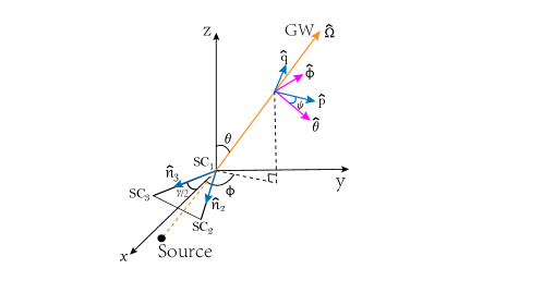
Figure 1: The detector frame. GWs propagate along $\hat{\Omega}$, and the laser beam transmits between the spacecrafts. The unit vector $\hat{n}_{2}$ is from the spacecraft $SC_{1}$ to the spacecraft $SC_{2}$, and the unit vector $\hat{n}_{3}$ is from the spacecraft $SC_{1}$ to the spacecraft $SC_{3}$. The arm lengths between the spacecrafts are $L$.

III.1 Basis vectors

For GWs propagating along the direction $\hat{\Omega}$, we use two perpendicular unit vectors $\hat{\theta}$ and $\hat{\phi}$ to form an orthonormal coordinate system, such that $\hat{\Omega}=\hat{\theta}\times\hat{\phi}$. In the detector coordinate system, we get

$$\begin{split}\hat{\theta}=&(\cos\theta\cos\phi,\cos\theta\sin\phi,-\sin\theta),\\ \hat{\phi}=&(-\sin\phi,\cos\phi,0),\\ \hat{\Omega}=&(\sin\theta\cos\phi,\sin\theta\sin\phi,\cos\theta).\end{split}$$ (11)

The two unit arm vectors are

$$\begin{split}\hat{n}_{2}=&(\cos\frac{\gamma}{2},\sin\frac{\gamma}{2},0),\\ \hat{n}_{3}=&(\cos\frac{\gamma}{2},-\sin\frac{\gamma}{2},0),\end{split}$$ (12)

where $\gamma$ is the angle between the interferometer’s two arms. Therefore, we get

$$\begin{split}\mu_{2}=\hat{n}_{2}\cdot\hat{\Omega}=\sin\theta\cos\phi_{-},\\ \mu_{3}=\hat{n}_{3}\cdot\hat{\Omega}=\sin\theta\cos\phi_{+},\end{split}$$ (13)

where $\phi_{+}=\phi+\gamma/2,\phi_{-}=\phi-\gamma/2$. For the convenience of calculation, we introduce $x=\mu_{2}$ and $y=\mu_{3}$.

III.2 The arm scalars

To account for the rotational degree of freedom around $\hat{\Omega}$, we introduce the polarization angle $\psi$ to form two new orthonormal vectors $\hat{p}$ and $\hat{q}$,

$$\begin{split}\hat{p}=&\cos\psi\hat{\theta}+\sin\psi\hat{\phi},\\ \hat{q}=&-\sin\psi\hat{\theta}+\cos\psi\hat{\phi}.\end{split}$$ (14)

With the orthonormal vectors $(\hat{p},\hat{q},\hat{\Omega})$, the six polarization tensors are defined as

$$\begin{split}e^{+}_{ij}=\hat{p}_{i}\hat{p}_{j}-\hat{q}_{i}\hat{q}_{j},\qquad&e^{\times}_{ij}=\hat{p}_{i}\hat{q}_{j}+\hat{q}_{i}\hat{p}_{j},\\ e^{x}_{ij}=\hat{p}_{i}\hat{\Omega}_{j}+\hat{\Omega}_{i}\hat{p}_{j},\qquad&e^{y}_{ij}=\hat{q}_{i}\hat{\Omega}_{j}+\hat{\Omega}_{i}\hat{q}_{j},\\ e^{b}_{ij}=\hat{p}_{i}\hat{p}_{j}+\hat{q}_{i}\hat{q}_{j},\qquad&e^{l}_{ij}=\hat{\Omega}_{i}\hat{\Omega}_{j}.\end{split}$$ (15)

Now we can calculate the variable $\zeta_{i}^{A}$.

III.2.1 The tensor mode

For the plus and cross modes, we get

$$\zeta^{+}_{2}=\sum_{i,j}\hat{n}_{2}^{i}\hat{n}_{2}^{j}e_{ij}^{+}=(\cos^{2}\theta\cos^{2}\phi_{-}-\sin^{2}\phi_{-})\cos(2\psi)-\cos\theta\sin(2\phi_{-})\sin(2\psi),$$ (16)

$$\zeta^{\times}_{2}=\sum_{i,j}\hat{n}_{2}^{i}\hat{n}_{2}^{j}e_{ij}^{\times}=-\cos\theta\sin(2\phi_{-})\cos(2\psi)-(\cos^{2}\theta\cos^{2}\phi_{-}-\sin^{2}\phi_{-})\sin(2\psi),$$ (17)

$$\zeta^{+}_{3}=\sum_{i,j}\hat{n}_{3}^{i}\hat{n}_{3}^{j}e_{ij}^{+}=(\cos^{2}\theta\cos^{2}\phi_{+}-\sin^{2}\phi_{+})\cos(2\psi)-\cos\theta\sin(2\phi_{+})\sin(2\psi),$$ (18)

$$\zeta^{\times}_{3}=\sum_{i,j}\hat{n}_{3}^{i}\hat{n}_{3}^{j}e_{ij}^{\times}=-\cos\theta\sin(2\phi_{+})\cos(2\psi)-(\cos^{2}\theta\cos^{2}\phi_{+}-\sin^{2}\phi_{+})\sin(2\psi).$$ (19)

Since we are interested in the average response function for the combined tensor mode $F^{T}=\sqrt{\left|F^{+}\right|^{2}+\left|F^{\times}\right|^{2}}$, we use the following arm scalars:

$$\begin{split}(\zeta^{T}_{2})^{2}=&(\zeta^{+}_{2})^{2}+(\zeta^{\times}_{2})^{2}=(1-x^{2})^{2},\\ (\zeta^{T}_{3})^{2}=&(\zeta^{+}_{3})^{2}+(\zeta^{\times}_{3})^{2}=(1-y^{2})^{2},\\ \zeta^{T}_{2}\zeta^{T}_{3}=&\zeta^{+}_{2}\zeta^{+}_{3}+\zeta^{\times}_{2}\zeta^{\times}_{3}=(1-x^{2})(1-y^{2})-2\sin^{2}\gamma\cos^{2}\theta.\end{split}$$ (20)

III.2.2 The vector mode

For the vector mode, we are interested in the average response function for the combined vector mode $F^{V}=\sqrt{|F^{x}|^{2}+|F^{y}|^{2}}$. Combining Eqs. (11)-(15), it is easy to get

$$\begin{split}(\zeta^{V}_{2})^{2}=&(\zeta^{x}_{2})^{2}+(\zeta^{y}_{2})^{2}=4x^{2}(1-x^{2}),\\ (\zeta^{V}_{3})^{2}=&(\zeta^{x}_{3})^{2}+(\zeta^{y}_{3})^{2}=4y^{2}(1-y^{2}),\\ \zeta^{V}_{2}\zeta^{V}_{3}=&\zeta^{x}_{2}\zeta^{x}_{3}+\zeta^{y}_{2}\zeta^{y}_{3}=4xy(\cos\gamma-xy).\end{split}$$ (21)

III.2.3 The breathing mode

For the breathing mode, combining Eqs. (11)-(15), we get

$$\begin{split}(\zeta^{b}_{2})^{2}=&(1-x^{2})^{2},\\ (\zeta^{b}_{3})^{2}=&(1-y^{2})^{2},\\ \zeta^{b}_{2}\zeta^{b}_{3}=&(1-x^{2})(1-y^{2}).\end{split}$$ (22)

III.2.4 The longitudinal mode

For the longitudinal mode, combining Eqs. (11)-(15), we get

$$\begin{split}(\zeta^{l}_{2})^{2}=&x^{4},\\ (\zeta^{l}_{3})^{2}=&y^{4},\\ \zeta^{l}_{2}\zeta^{l}_{3}=&x^{2}y^{2}.\end{split}$$ (23)

III.3 The averaged response function

The averaged response (transfer) function is defined as

$$R^{A}=\frac{1}{8\pi^{2}}\int_{0}^{\pi}\sin\theta d\theta\int_{0}^{2\pi}d\phi\int_{0}^{2\pi}d\psi\left|F^{A}\right|^{2}.$$ (24)

Note that $\left|F^{A}\right|^{2}$ for the tensor, vector, breathing, and longitudinal modes does not contain the polarization angle $\psi$ and $R^{+}=R^{\times}=R^{T}/2,R^{x}=R^{y}=R^{V}/2$ Liang et al. (2019); it is unnecessary to integrate over $\psi$ for these modes. Thus, the averaged response function becomes

$$\begin{split}R^{A}=&\frac{1}{4\pi}\int_{0}^{\pi}\sin\theta d\theta\int_{0}^{2\pi}d\phi\left|F^{A}\right|^{2}\\ =&\frac{1}{2\pi}\int_{-1}^{1}dy\int_{y\cos\gamma-\sin\gamma\sqrt{1-y^{2}}}^{y\cos\gamma+\sin\gamma\sqrt{1-y^{2}}}dx\frac{\left|F^{A}\right|^{2}}{\sqrt{\sin^{2}\gamma-x^{2}-y^{2}+2xy\cos\gamma}}.\end{split}$$ (25)

In the above derivation, we change the integral variables $\theta$ and $\phi$ by $x=\sin\theta\cos(\phi-\gamma/2)$ and $y=\sin\theta\cos(\phi+\gamma/2)$. Plugging Eq. (7) into Eq. (25), we get

$$\begin{split}u^{2}R^{A}_{MI}=&\frac{1}{2\pi}\int_{-1}^{1}dy\int_{y\cos\gamma-\sin\gamma\sqrt{1-y^{2}}}^{y\cos\gamma+\sin\gamma\sqrt{1-y^{2}}}\frac{dx}{\sqrt{\sin^{2}\gamma-x^{2}-y^{2}+2xy\cos\gamma}}\\ &\left\{\frac{2x^{2}+(1-x^{2})\sin^{2}u-2x\sin u\sin(ux)-2x^{2}\cos u\cos(ux)}{4(1-x^{2})^{2}}(\zeta_{2}^{A})^{2}\right.\\ &+\frac{2y^{2}+(1-y^{2})\sin^{2}u-2y\sin u\sin(uy)-2y^{2}\cos u\cos(uy)}{4(1-y^{2})^{2}}(\zeta_{3}^{A})^{2}\\ &\left.-\frac{\eta(u,x,y)}{2(1-x^{2})(1-y^{2})}\zeta_{2}^{A}\zeta_{3}^{A}\right\},\end{split}$$ (26)

where

$$\begin{split}\eta(u,x,y)=&\sin^{2}u-[x\sin(ux)+y\sin(uy)]\sin u+xy\cos[u(x-y)]\\ &+xy[\cos^{2}u-\cos u\cos(ux)-\cos u\cos(uy)].\end{split}$$ (27)

Because of the relation $\left|F^{A}_{MC}\right|^{2}=16\sin^{2}u\left|F^{A}_{MI}\right|^{2}$,

$$R^{A}_{MC}=16\sin^{2}(u)R^{A}_{MI}.$$ (28)

Substituting the results in Eqs. (20),(21),(22), and (23) into Eq. (26), we can derive the analytical expressions. The detailed calculations are presented in the Appendix.

IV The full analytical formalism

In this section, we present the full analytical formulas of the averaged response functions for interferometric GW detectors without optical cavities. We also give asymptotic behaviors for these averaged response functions.

IV.1 The tensor mode

The analytical formula of the averaged response function for the combined tensor mode is

$$\begin{split}u^{2}R^{T}_{MI}=&\frac{3-\cos\gamma}{12}+\frac{-1+\cos\gamma}{u^{2}}+2\sin^{2}\left(\frac{\gamma}{2}\right)\Big{[}\text{Ci}\left[2u\sin\left(\frac{\gamma}{2}\right)\right]-\ln\left[\sin\left(\frac{\gamma}{2}\right)\right]\\ &-\text{Ci}(2u)\Big{]}+\frac{1+\csc^{2}\left(\frac{\gamma}{2}\right)}{8u^{2}}\cos\left[2u\sin\left(\frac{\gamma}{2}\right)\right]+\sin\left[2u\sin\left(\frac{\gamma}{2}\right)\right]\left[\frac{-3+\cos\gamma}{32u^{3}}\right.\\ &\left.+\frac{-21+28\cos\gamma-7\cos(2\gamma)}{32u}\right]\csc^{3}\left(\frac{\gamma}{2}\right)+\sin(2u)\left[\left(\frac{1}{u}+\frac{2}{u^{3}}\right)\sin^{2}\left(\frac{\gamma}{2}\right)\right.\\ &\left.+\cos^{2}\left(\frac{\gamma}{2}\right)\Big{(}2\text{Si}(2u)-\text{Si}\left[2u+2u\sin\left(\frac{\gamma}{2}\right)\right]-\text{Si}\left[2u-2u\sin\left(\frac{\gamma}{2}\right)\right]\Big{)}\right]\\ &+\Big{[}\cos^{2}\left(\frac{\gamma}{2}\right)\Big{(}2\text{Ci}(2u)+\ln\left[\cos^{2}\left(\frac{\gamma}{2}\right)\right]-\text{Ci}\left[2u+2u\sin\left(\frac{\gamma}{2}\right)\right]\\ &-\text{Ci}\left[2u-2u\sin\left(\frac{\gamma}{2}\right)\right]\Big{)}+\left(\frac{1}{6}-\frac{2}{u^{2}}\right)\sin^{2}\left(\frac{\gamma}{2}\right)\Big{]}\cos(2u),\end{split}$$ (29)

where $\gamma_{E}$ is the Euler constant, $\text{Si}(u)$ is sine-integral function, and $\text{Ci}(u)$ is cosine-integral function. Using the analytical expression (29), we plot $R^{T}_{MI}$ in Fig. 2, and the plot can be done in less than a second on a desktop or laptop computer for 500 data points with $\log(u)$ uniformly distributed from 0.001 to 100. If we use the semianalytical formula Larson et al. (2000); Liang et al. (2019), we need about 6 min to plot the figure as shown with the dotted line in Fig. 2. Of course, if we plot more data points, it takes more time. The analytical and semianalytical formulae give the same results as shown in Fig. 2. Therefore, the full analytical expression is much more efficient for the calculation of the transfer function.

In the low frequency limit, $u\ll 1$,

$$\begin{split}{\rm Si}(2u)\to 2u-\frac{4u^{3}}{9}+\frac{4u^{5}}{75}+o(u^{7}),\\ {\rm Ci}(2u)\to\ln(2u)+\gamma_{E}-u^{2}+\frac{u^{4}}{6}-\frac{2u^{6}}{135}+o(u^{8}).\end{split}$$ (30)

$$R^{T}_{MI}\to\frac{2}{5}\sin^{2}\gamma.$$ (31)

Note that $\sin(u)/u\to 1$ as $u\to 0$; the terms involving $1/u^{2}$, $\cos(u)/u^{2}$, and $\sin(u)/u^{3}$ cancel out, and the terms with $\sin(u)/u$ cancel out the first constant term in Eq. (29), so the lowest order is $u^{2}$ in the right-hand side of Eq. (29). In the high frequency limit, $u\gg 1$,

$$\begin{split}{\rm Si}(u)\to\frac{\pi}{2}-\frac{\cos(u)}{u}+o(\frac{1}{u^{2}}),\\ {\rm Ci}(u)\to\frac{\sin(u)}{u}+o(\frac{1}{u^{2}}).\end{split}$$ (32)

$$R^{T}_{MI}\to R^{T}_{h1}+R^{T}_{h2},$$ (33)

where

$$R^{T}_{h1}=\left[\frac{3-\cos\gamma}{12}-2\sin^{2}\left(\frac{\gamma}{2}\right)\ln\left(\sin\frac{\gamma}{2}\right)\right]\frac{1}{u^{2}},$$ (34)

and

$$R^{T}_{h2}=\left[\frac{1}{6}\sin^{2}\left(\frac{\gamma}{2}\right)+\cos^{2}\left(\frac{\gamma}{2}\right)\ln\left[\cos^{2}\left(\frac{\gamma}{2}\right)\right]\right]\frac{\cos(2u)}{u^{2}}.$$ (35)

To approximate the averaged response function (29), the following analytical expression for LISA was widely used Robson et al. (2019):

$$R^{T}\approx\frac{3}{10}\frac{1}{1+0.6(f/f_{*})^{2}}.$$ (36)

In Babak et al. (2007), they used the approximation,

$$R^{T}\approx\frac{9}{16(f/f_{*})^{2}}\left[\left(\frac{1}{3}-\frac{2}{(f/f_{*})^{2}}\right)[1+\cos^{2}(f/f_{*})]+\sin^{2}(f/f_{*})+\frac{2\sin(2f/f_{*})}{(f/f_{*})^{3}}\right],$$ (37)

which is the analytical part (56) of the semianalytical expression for the averaged response function derived in Larson et al. (2000). An overall factor of 9/8 is added to the expression so that the low frequency limit is recovered. It is a coincidence that both the low and high frequency limits are recovered with the same overall factor. However, for the vector, breathing, and longitudinal modes, the analytical part in the semianalytical formulas cannot be used to approximate the full analytical expression because the overall factors for the low and high frequency limits are different.

Based on the expression (29) and its low frequency behavior (31) and high frequency behavior (33), for quick estimation we suggest the following analytical approximation:

$$R^{T}_{MI}\approx\frac{2}{5}\sin^{2}\gamma\left[1+\frac{2\sin^{2}\gamma}{5(R^{T}_{h1}+R^{T}_{h2})}\right]^{-1}.$$ (38)

Take $\gamma=\pi/3$, the approximation (38) becomes

$$R^{T}_{MI}\approx\frac{3}{10}\frac{1}{1+(f/f_{*})^{2}/[1.85-0.58\cos(2f/f_{*})]}.$$ (39)

The approximations (36), (37), and (39) are shown in Fig. 3. It is interesting that the approximation (37) is more accurate.

IV.2 The vector mode

The analytical formula of the averaged response functions for the combined vector mode is

$$\begin{split}u^{2}R^{V}_{MI}=&-4+\frac{4\cos\gamma}{3}+\frac{4-4\cos\gamma}{u^{2}}+2\left[\gamma_{E}-\text{Ci}\left[2u\sin\left(\frac{\gamma}{2}\right)\right]+\ln\left[2u\sin\left(\frac{\gamma}{2}\right)\right]\right]\\ &-\frac{1+\csc^{2}\left(\frac{\gamma}{2}\right)}{2u^{2}}\cos\left[2u\sin\left(\frac{\gamma}{2}\right)\right]+\sin\left[2u\sin\left(\frac{\gamma}{2}\right)\right]\left[\frac{7-8\cos\gamma+\cos(2\gamma)}{8u}\right.\\ &+\left.\frac{3-\cos\gamma}{8u^{3}}\right]\csc^{3}\left(\frac{\gamma}{2}\right)+\left[\left(\frac{4}{u}-\frac{8}{u^{3}}\right)\sin^{2}\left(\frac{\gamma}{2}\right)+\text{Si}\left[2u+2u\sin\left(\frac{\gamma}{2}\right)\right]\right.\\ &\left.-2\text{Si}(2u)+\text{Si}\left[2u-2u\sin\left(\frac{\gamma}{2}\right)\right]\right]\sin(2u)+\left[\left(\frac{8}{u^{2}}-\frac{8}{3}\right)\sin^{2}\left(\frac{\gamma}{2}\right)-2\text{Ci}(2u)\right.\\ &\left.+\text{Ci}\left[2u+2u\sin\left(\frac{\gamma}{2}\right)\right]+\text{Ci}\left[2u-2u\sin\left(\frac{\gamma}{2}\right)\right]-\ln\left[\cos^{2}\left(\frac{\gamma}{2}\right)\right]\right]\cos(2u).\end{split}$$ (40)

Using the analytical expression (40), we plot $R^{V}_{MI}$ in Figs. 2 and 3.

In the low frequency limit $u\ll 1$,

$$R^{V}_{MI}\to\frac{2}{5}\sin^{2}\gamma.$$ (41)

In the low frequency limit, the terms involving $1/u^{2}$, $\cos(u)/u^{2}$, and $\sin(u)/u^{3}$ cancel out, and the terms with $\sin(u)/u$ cancel out the first constant terms in Eq. (40), so $R^{V}_{MI}$ approaches to a constant. In the high frequency, limit $u\gg 1$,

$$\begin{split}R^{V}_{MI}\to R^{V}_{h}=&\frac{2}{u^{2}}\left[\ln\left[\frac{3}{u}+2u\sin\left(\frac{\gamma}{2}\right)\right]-2+\frac{2}{3}\cos\gamma+\gamma_{E}\right]\\ &-\frac{\cos(2u)}{u^{2}}\left[\frac{8}{3}\sin^{2}\left(\frac{\gamma}{2}\right)+\ln\left[\cos^{2}\left(\frac{\gamma}{2}\right)\right]\right].\end{split}$$ (42)

For a quick estimation, based on the low and high frequency limits, we may use the approximation,

$$R^{V}_{MI}\approx\frac{2}{5}\sin^{2}\gamma\left[1+\frac{2\sin^{2}\gamma}{5R^{V}_{h}}\right]^{-1}.$$ (43)

Take $\gamma=\pi/3$, the approximation (43) becomes

$$R^{V}_{MI}\approx\frac{3}{10}\frac{1}{1+(f/f_{*})^{2}/[-7.26-1.26\cos(2f/f_{*})+6.67\ln(3f_{*}/f+f/f_{*})]}.$$ (44)

As shown in Fig. 3, the above expression (44) approximates the analytical result (40) well.

IV.3 The breathing mode

The analytical formula of the averaged response function for the breathing mode is

$$\begin{split}u^{2}R^{b}_{MI}=&\frac{3-\cos\gamma}{12}+\frac{-1+\cos\gamma}{u^{2}}+\sin(2u)\left(\frac{2}{u^{3}}-\frac{1}{u}\right)\sin^{2}\left(\frac{\gamma}{2}\right)\\ &+\sin\left[2u\sin\left(\frac{\gamma}{2}\right)\right]\csc^{3}\left(\frac{\gamma}{2}\right)\left[\frac{\cos\gamma-3}{32u^{3}}+\frac{3-4\cos\gamma+\cos(2\gamma)}{32u}\right]\\ &+\cos(2u)\left(\frac{1}{6}-\frac{2}{u^{2}}\right)\sin^{2}\left(\frac{\gamma}{2}\right)+\cos\left[2u\sin\left(\frac{\gamma}{2}\right)\right]\frac{1+\csc^{2}\left(\frac{\gamma}{2}\right)}{8u^{2}}.\end{split}$$ (45)

Using the analytical expression (45), we plot $R^{b}_{MI}$ in Figs. 2 and 3.

In the low frequency limit $u\ll 1$, we get

$$R^{b}_{MI}\to\frac{1}{15}\sin^{2}\gamma.$$ (46)

In the low frequency limit, the terms involving $1/u^{2}$, $\cos(u)/u^{2}$, and $\sin(u)/u^{3}$ cancel out, and the terms with $\sin(u)/u$ cancel out the first constant term in Eq. (45), so $R^{b}_{MI}$ approaches to a constant. In the high frequency limit $u\gg 1$, we get

$$R^{b}_{MI}\to\frac{3-\cos\gamma+(1-\cos\gamma)\cos(2u)}{12u^{2}}.$$ (47)

For a quick estimation, combining the low and high frequency limits, we may use the approximation,

$$R^{b}_{MI}\approx\frac{1}{15}\sin^{2}\gamma\left[1+\frac{4u^{2}\sin^{2}\gamma}{5[3-\cos\gamma+(1-\cos\gamma)\cos(2u)]}\right]^{-1}.$$ (48)

Take $\gamma=\pi/3$, the approximation (48) becomes

$$R^{b}_{MI}\approx\frac{1}{20}\frac{1}{1+(f/f_{*})^{2}/[4.17+0.83\cos(2f/f_{*})]}.$$ (49)

As shown in Fig. 3, the above expression (49) approximates the analytical result (45) well.

IV.4 The longitudinal mode

The analytical formula of the averaged response functions for the longitudinal mode is

$$\begin{split}u^{2}R^{l}_{MI}=&\frac{13}{8}-\frac{7\cos\gamma}{12}+\frac{-1+\cos\gamma}{u^{2}}+\frac{u}{4}\text{Si}(2u)+\left[-\frac{7}{8}+\frac{\cos\gamma}{4}+\frac{\csc^{2}\left(\frac{\gamma}{2}\right)}{8}\right]\left[\gamma_{E}\right.\\ &\left.-\text{Ci}(2u)+\ln(2u)\right]-\frac{1}{4}\left[\gamma_{E}-\text{Ci}\left[2u\sin\left(\frac{\gamma}{2}\right)\right]+\ln\left[2u\sin\left(\frac{\gamma}{2}\right)\right]\right]\csc^{2}\left(\frac{\gamma}{2}\right)\\ &+\frac{1+\csc^{2}\left(\frac{\gamma}{2}\right)}{8u^{2}}\cos\left[2u\sin\left(\frac{\gamma}{2}\right)\right]+\sin\left[2u\sin\left(\frac{\gamma}{2}\right)\right]\csc^{3}\left(\frac{\gamma}{2}\right)\left[\frac{-3+\cos\gamma}{32u^{3}}\right.\\ &\left.+\frac{-5+4\cos\gamma+\cos 2\gamma}{32u}\right]+\frac{1}{2}\cos\gamma\cot^{2}\gamma\left[\sin\left[2u\sin^{2}\left(\frac{\gamma}{2}\right)\right]\left(\text{Si}\left[2u\sin^{2}\left(\frac{\gamma}{2}\right)\right]\right.\right.\\ &+\text{Si}\left[2u\sin\left(\frac{\gamma}{2}\right)-2u\sin^{2}\left(\frac{\gamma}{2}\right)\right]-\text{Si}\left[2u\sin\left(\frac{\gamma}{2}\right)+2u\sin^{2}\left(\frac{\gamma}{2}\right)\right]\\ &\left.-\text{Si}\left[2u\cos^{2}\left(\frac{\gamma}{2}\right)\right]\right)+\cos\left[2u\sin^{2}\left(\frac{\gamma}{2}\right)\right]\Big{(}\text{Ci}\left[2u\sin^{2}\left(\frac{\gamma}{2}\right)\right]+\text{Ci}\left[2u\cos^{2}\left(\frac{\gamma}{2}\right)\right]\\ &\left.-\text{Ci}\left[2u\sin\left(\frac{\gamma}{2}\right)-2u\sin^{2}\left(\frac{\gamma}{2}\right)\right]-\text{Ci}\left[2u\sin\left(\frac{\gamma}{2}\right)+2u\sin^{2}\left(\frac{\gamma}{2}\right)\right]\Big{)}\right]\\ &+\frac{\sec^{2}\left(\frac{\gamma}{2}\right)}{16}\left[\left(\frac{8}{u^{3}}-\frac{8}{u}\right)\sin^{2}\gamma-2\text{Si}\left[2u-2u\sin\left(\frac{\gamma}{2}\right)\right]-2\text{Si}\left[2u+2u\sin\left(\frac{\gamma}{2}\right)\right]\right.\\ &+[4+\cos\gamma-\cos(2\gamma)]\text{Si}(2u)\Big{]}\sin(2u)+\frac{\sec^{2}\left(\frac{\gamma}{2}\right)}{16}\left[\frac{10+3\cos\gamma-7\cos(2\gamma)}{3}\right.\\ &+\frac{-4+4\cos 2\gamma}{u^{2}}-[\cos\gamma-\cos(2\gamma)]\gamma_{E}+[4+\cos\gamma-\cos(2\gamma)]\left[\text{Ci}(2u)-\ln(2u)\right]\\ &-\left.2\text{Ci}\left[2u-2u\sin\left(\frac{\gamma}{2}\right)\right]-2\text{Ci}\left[2u+2u\sin\left(\frac{\gamma}{2}\right)\right]+4\ln\left[2u\cos\left(\frac{\gamma}{2}\right)\right]\right]\cos(2u).\end{split}$$ (50)

Using the analytical expression (50), we plot $R^{l}_{MI}$ in Figs. 2 and 3.

In the low frequency limit, $u\ll 1$,

$$R^{l}_{MI}\to\frac{1}{15}\sin^{2}\gamma.$$ (51)

$R^{l}_{MI}$ approaches to a constant because the terms involving $1/u^{2}$, $\cos(u)/u^{2}$, and $\sin(u)/u^{3}$ cancel out, and the $\sin(u)/u$ terms cancel out the first constant terms in Eq. (50) in the low frequency limit. In the high frequency limit, $u\gg 1$,

$$\begin{split}R^{l}_{MI}\to R^{l}_{h}=&\frac{\pi}{8u}+\frac{1}{16u^{2}}-\frac{\ln(2u)}{16u^{2}}\left[3+2\csc^{2}\left(\frac{\gamma}{2}\right)-4\cos\gamma\right.\\ &\left.\quad+\sec^{2}\left(\frac{\gamma}{2}\right)[\cos\gamma-\cos(2\gamma)]\cos(2u)\right].\end{split}$$ (52)

For a quick estimation, based on the low and high frequency limits, we suggest the following approximation:

$$R^{l}_{MI}\approx\frac{1}{15}\sin^{2}\gamma\left[1+\frac{\sin^{2}\gamma}{15R^{l}_{h}}\right]^{-1}.$$ (53)

Take $\gamma=\pi/3$, we get

$$R^{l}_{MI}\approx\frac{1}{20}\frac{1}{1+(f/f_{*})^{2}/[1.25+7.85f/f_{*}-(11.25+1.67\cos(2f/f_{*}))\ln(2f/f_{*})]}.$$ (54)

As shown in Fig. 3, the above expression (54) approximates the analytical result (50) well.

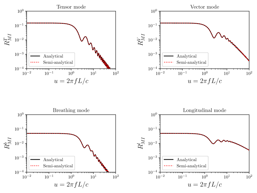
Figure 2: The averaged response functions of different polarizations by using the analytical and semianalytical formulas for interferometric GW detectors without optical cavities in the arms. We take $\gamma=\pi/3$. With the analytical expressions, we can plot this figure in less than 3 sec, but it takes more than 40 min to plot this figure if we use the semianalytical formulas derived in Liang et al. (2019). The code for the plot and the transfer functions is available at %****␣analytical.tex␣Line␣700␣****https://github.com/yggong/transfer_function.

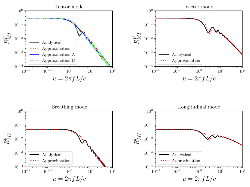
Figure 3: The averaged response functions of different polarizations by using the analytical and approximate formulas for interferometric GW detectors without optical cavities in the arms. We take $\gamma=\pi/3$. In the upper left panel, the approximation uses the formula (39), the approximation A uses the formula (36), and the approximation B uses the formula (37).

To obtain the analytical expressions of the transfer functions for the equal arm Michelson combinations, we use the relation $R^{A}_{MC}=16\sin^{2}(u)R^{A}_{MI}$. The results along with their approximations are shown in Fig. 4.

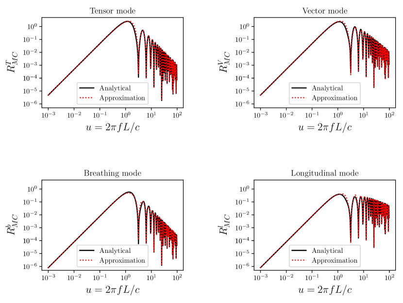
Figure 4: The analytical formulas of the averaged response functions for TDI Michelson combination and their approximations with Eqs. (39), (44), (49), and (54) multiplied by $16\sin^{2}(u)$. We take $\gamma=\pi/3$ in the plots.

V Conclusions

For the space-based interferometric GW detectors without optical cavities in the arms, such as LISA, TaiJi, and TianQin, we derive the full analytical formulas for the frequency dependent response functions for the tensor, vector, breathing, and longitudinal polarizations. These analytical expressions are consistent with those obtained by Monte Carlo simulation and the semianalytical results we derived before. With these analytical formulas, the evaluation of the ability of the detector becomes easier and faster. In particular, the calculation of the signal to noise ratio for a space-based GW detector becomes more efficient. We also find that for space-based interferometric GW detectors, the averaged response functions of the equal arm TDI Michelson combination are just the derived results multiplied by $16\sin^{2}u$.

With these analytical expressions, the asymptotic behaviors in the low and high frequency limits are apparent. In particular, we can derive analytical expressions for the high frequency behaviors so that the high frequency behaviors can be easily understood. For the tensor and breathing modes, the average response functions fall off as $1/f^{2}$ at high frequencies, and they also oscillate due to the factor $\cos(2f/f_{*})$. At high frequencies, $f\gg f_{*}=c/(2\pi L)$, the averaged response functions decrease as $\ln(f)/f^{2}$ for the vector mode and $1/f$ for the longitudinal mode. Even though they also have the term with $\cos(2f/f_{*})$, the oscillation is suppressed by a factor of $1/\ln(f)$ or $\ln(f)/f$. For the vector mode, the oscillation falls off as $1/f^{2}$, but the dominant contribution falls off as $\ln(f)/f^{2}$. For the longitudinal mode, the oscillation falls off as $\ln(f)/f^{2}$, but the dominant contribution falls off as $1/f$. For the equal arm TDI Michelson combination, due to the factor $\sin^{2}u$, at low frequencies, the averaged response functions increase as $f^{2}$. At high frequencies, they oscillate as $\sin^{2}(f/f_{*})$.

Combining the asymptotic behaviors in the low and high frequency limits, we give simple approximate expressions for the averaged response functions. Our approximate expressions to calculate the averaged response functions provide a quick evaluation of the GW detector ability and efficient estimation of the signal to noise ratio. The derived full analytical formulas are useful in space-based GW detection and the test of theory of gravity.

Appendix A Detailed calculations for the transfer functions

Because the integration region $x^{2}+y^{2}-2xy\cos\gamma\leq\sin^{2}\gamma$ is symmetric for $x$ and $y$, we can interchange $x$ and $y$ in the integrand. Thus, the first two integrands involving $(\zeta_{2}^{A})^{2}$ and $(\zeta_{3}^{A})^{2}$ in Eq. (26) give the same results. For the last term with $\zeta^{A}_{2}\zeta^{A}_{3}$, the integration of $xy\cos(ux)$ in $\eta(u,x,y)$ is the same as that of $xy\cos(uy)$, and the integration of $x\sin(ux)$ in $\eta(u,x,y)$ is the same as that of $y\sin(uy)$. Therefore, we can rewrite $\eta(u,x,y)$ as

$$\begin{split}\eta(u,x,y)=&\sin^{2}u+xy[\cos^{2}u-2\cos u\cos(ux)]-2x\sin(ux)\sin u\\ &+xy\cos[u(x-y)].\end{split}$$ (55)

To calculate the last term in Eq. (26), we integrate the two lines in Eq. (55) separately.

A.1 The breathing mode

Substituting Eq. (22) into Eq. (26), the first two integrations in Eq. (26) are Liang et al. (2019)

$$\begin{split}I_{b1}&=\int_{-1}^{1}dy\int_{y_{l}}^{y_{u}}dx\frac{2y^{2}+(1-y^{2})\sin^{2}u-2y\sin u\sin(uy)-2y^{2}\cos u\cos(uy)}{4\pi\sqrt{\sin^{2}\gamma-x^{2}-y^{2}+2xy\cos\gamma}}\\ &=\frac{1}{2}\left(\frac{1}{3}-\frac{2}{u^{2}}\right)(1+\cos^{2}u)+\frac{1}{2}\sin^{2}u+\frac{\sin(2u)}{u^{3}},\end{split}$$ (56)

where $y_{l}=y\cos\gamma-\sin\gamma\sqrt{1-y^{2}}$ and $y_{u}=y\cos\gamma+\sin\gamma\sqrt{1-y^{2}}$. This is the analytical part of the semianalytical formulas obtained in Liang et al. (2019).

For the integration of the last term in Eq. (26) isolating the term $xy\cos(ux-uy)$ in $\eta(u,x,y)$, and using the symmetry of $x$ and $y$, we get

$$\begin{split}I_{b2}=&-\int_{-1}^{1}dy\int_{y_{l}}^{y_{u}}dx\frac{\sin^{2}u+xy\cos^{2}u-2xy\cos u\cos(uy)-2y\sin u\sin(uy)}{4\pi\sqrt{\sin^{2}\gamma-x^{2}-y^{2}+2xy\cos\gamma}}\\ =&-\frac{1}{4}-\frac{\cos\gamma}{12}+\frac{1+2\cos\gamma}{2u^{2}}+\left(\frac{3-\cos\gamma}{12}-\frac{1-2\cos\gamma}{2u^{2}}\right)\cos(2u)\\ &-\left(\frac{\cos\gamma}{u^{3}}+\frac{1-\cos\gamma}{2u}\right)\sin(2u).\end{split}$$ (57)

To calculate the integration of $xy\cos(ux-uy)$, we change the variables $x$ and $y$ to $a=(x+y)/2$ and $b=(x-y)/2$. After the change of integration variables, the integration is

$$\begin{split}I_{b3}=&-\int_{-1}^{1}dy\int_{y_{l}}^{y_{u}}dx\frac{xy\cos(ux-uy)}{4\pi\sqrt{\sin^{2}\gamma-x^{2}-y^{2}+2xy\cos\gamma}}\\ =&-\int_{-\sin\frac{\gamma}{2}}^{\sin\frac{\gamma}{2}}db\int_{-a_{l}}^{a_{l}}da\frac{(a^{2}-b^{2})\cos(2ub)}{2\pi\sqrt{\sin^{2}(\gamma)-4\sin^{2}(\frac{\gamma}{2})a^{2}-4\cos^{2}(\frac{\gamma}{2})b^{2}}}\\ =&\left(\frac{3-4\cos\gamma+\cos(2\gamma)}{32u}-\frac{3-\cos\gamma}{32u^{3}}\right)\csc^{3}\left(\frac{\gamma}{2}\right)\sin\left[2u\sin\left(\frac{\gamma}{2}\right)\right]\\ &+\frac{1+\csc^{2}\left(\frac{\gamma}{2}\right)}{8u^{2}}\cos\left[2u\sin\left(\frac{\gamma}{2}\right)\right],\end{split}$$ (58)

where $a_{l}=\cos(\gamma/2)\sqrt{1-[b/\sin(\gamma/2)]^{2}}$. Add Eqs. (56)-(58) together, we get the analytical formula (45) for the breathing mode. Note that

$$I_{b2}+I_{b3}=-\frac{1}{8\pi}\int_{0}^{2\pi}d\epsilon\int_{0}^{\pi}d\theta_{1}\sin\theta\eta(u,\tilde{\mu}_{1},\tilde{\mu}_{2}),$$ (59)

where $\tilde{\mu}_{1}=\cos\theta_{1}$, $\tilde{\mu}_{2}=\cos\gamma\cos\theta_{1}+\sin\gamma\sin\theta_{1}\cos\epsilon$ Liang et al. (2017).

A.2 The tensor mode

Substituting Eq. (20) into Eq. (26), we get the first two integrations in Eq. (26) as

$$\begin{split}I_{T1}=I_{b1},\end{split}$$ (60)

which gives the analytical part of the semianalytical formulas in Larson et al. (2000); Liang et al. (2019).

For the third integration in Eq. (26), since $\zeta^{T}_{2}\zeta^{T}_{3}=(1-x^{2})(1-y^{2})-2\sin^{2}\gamma\cos^{2}\theta$, we integrate the term $(1-x^{2})(1-y^{2})$ first, and we get

$$\begin{split}I_{T2}=I_{b2}+I_{b3}.\end{split}$$ (61)

To integrate the term $-2\sin^{2}\gamma\cos^{2}\theta$, we use the result $\sin\gamma\cos\theta=\sqrt{\sin^{2}\gamma-x^{2}-y^{2}+2xy\cos\gamma}$, so

$$\begin{split}I_{T_{3}}=&\frac{1}{4\pi}\int_{0}^{2\pi}d\epsilon\int_{0}^{\pi}d\theta_{1}\sin\theta_{1}\frac{\sin^{2}\gamma\sin^{2}\epsilon}{1-\tilde{\mu_{2}}^{2}}\eta(u,\tilde{\mu}_{1},\tilde{\mu}_{2})\\ =&\int dxdy\frac{\eta(u,x,y)}{2\pi(1-x^{2})(1-y^{2})}\sqrt{\sin^{2}\gamma-x^{2}-y^{2}+2xy\cos\gamma}\\ =&\frac{-3+4\cos\gamma-\cos(2\gamma)}{4u}\sin\left[2u\sin\left(\frac{\gamma}{2}\right)\right]\csc^{3}\left(\frac{\gamma}{2}\right)+2\left[\text{Ci}\left[2u\sin\left(\frac{\gamma}{2}\right)\right]\right.\\ &\left.-\text{Ci}(2u)-\ln\left[\sin\left(\frac{\gamma}{2}\right)\right]\right]\sin^{2}\left(\frac{\gamma}{2}\right)+\left[\frac{2}{u}\sin^{2}\left(\frac{\gamma}{2}\right)-\left(\text{Si}\left[2u+2u\sin\left(\frac{\gamma}{2}\right)\right]\right.\right.\\ &\left.\left.-2\text{Si}(2u)+\text{Si}\left[2u-2u\sin\left(\frac{\gamma}{2}\right)\right]\right)\cos^{2}\left(\frac{\gamma}{2}\right)\right]\sin(2u)+\left[\ln\left[\cos^{2}\left(\frac{\gamma}{2}\right)\right]\right.\\ &\left.+2\text{Ci}(2u)-\text{Ci}\left[2u+2u\sin\left(\frac{\gamma}{2}\right)\right]-\text{Ci}\left[2u-2u\sin\left(\frac{\gamma}{2}\right)\right]\right]\cos^{2}\left(\frac{\gamma}{2}\right)\cos(2u).\end{split}$$ (62)

In the above integration, we follow the method used in the previous section that we separate $\eta(u,x,y)$ into two parts. Add Eqs. (60)-(62) together, we get the analytical formula Eq. (29) for the combined tensor mode.

A.3 The vector mode

Substituting Eq. (21) into Eq. (26), the integrations of the first two terms in Eq. (26) are Liang et al. (2019)

$$\begin{split}I_{V1}&=\int_{-1}^{1}dy\int_{y_{l}}^{y_{u}}dx\frac{2y^{2}+(1-y^{2})\sin^{2}u-2y\sin u\sin(uy)-2y^{2}\cos u\cos(uy)}{\pi(1-y^{2})\sqrt{\sin^{2}\gamma-x^{2}-y^{2}+2xy\cos\gamma}}y^{2}\\ &=-5+\frac{6}{u^{2}}+2\left[\gamma_{E}-\text{Ci}(2u)+\ln(2u)\right]+\left(\frac{2}{u}-\frac{4}{u^{3}}\right)\sin 2u+\left(\frac{2}{u^{2}}-\frac{1}{3}\right)\cos 2u.\end{split}$$ (63)

This is the analytical part of the semianalytical formulas obtained in Liang et al. (2019). Follow the same procedure, we get the integration of the last term in Eq. (26),

$$\begin{split}I_{V2}=&-\frac{1}{2\pi}\int_{0}^{\pi}d\theta_{1}\int_{0}^{2\pi}d\epsilon\frac{\cos\theta_{1}(-\sin\gamma\cos\theta_{1}\cos\epsilon+\cos\gamma\sin\theta_{1})\tilde{\mu}_{2}}{1-\tilde{\mu}_{2}^{2}}\eta(u,\tilde{\mu}_{1},\tilde{\mu}_{2})\\ =&-\int_{-1}^{1}dy\int_{y_{l}}^{y_{u}}dx\frac{xy(\cos\gamma-xy)\eta(u,x,y)}{\pi(1-x^{2})(1-y^{2})\sqrt{\sin^{2}\gamma-x^{2}-y^{2}+2xy\cos\gamma}}\\ =&1+\frac{4\cos\gamma}{3}-\frac{2+4\cos\gamma}{u^{2}}+2\left[\text{Ci}(2u)-\text{Ci}\left[2u\sin\left(\frac{\gamma}{2}\right)\right]+\ln\left[\sin\left(\frac{\gamma}{2}\right)\right]\right]\\ &+\frac{1+\csc^{2}\left(\frac{\gamma}{2}\right)}{2u^{2}}\cos\left[2u\sin\left(\frac{\gamma}{2}\right)\right]+\sin\left[2u\sin\left(\frac{\gamma}{2}\right)\right]\csc^{3}\left(\frac{\gamma}{2}\right)\left[\frac{3-\cos\gamma}{8u^{3}}\right.\\ &+\left.\frac{7-8\cos\gamma+\cos(2\gamma)}{8u}\right]+\left[\text{Si}\left[2u+2u\sin\left(\frac{\gamma}{2}\right)\right]+\text{Si}\left[2u-2u\sin\left(\frac{\gamma}{2}\right)\right]\right.\\ &\left.-2\text{Si}(2u)-\left(\frac{2}{u}-\frac{4}{u^{3}}\right)\cos\gamma\right]\sin 2u+\left[\frac{2-4\cos\gamma}{u^{2}}+\frac{-3+4\cos\gamma}{3}-2\text{Ci}(2u)\right.\\ &\left.+\text{Ci}\left[2u+2u\sin\left(\frac{\gamma}{2}\right)\right]+\text{Ci}\left[2u-2u\sin\left(\frac{\gamma}{2}\right)\right]-\ln\left[\cos^{2}\left(\frac{\gamma}{2}\right)\right]\right]\cos 2u.\end{split}$$ (64)

Add Eqs. (63)-(64) together, we get the analytical formula Eq. (40) for the vector mode.

A.4 The longitudinal mode

Substituting Eq. (23) into Eq. (26), the first two integrations in Eq. (26) are Liang et al. (2019)

$$\begin{split}I_{l1}=&\int_{-1}^{1}dy\int_{y_{l}}^{y_{u}}dx\frac{2y^{2}+(1-y^{2})\sin^{2}u-2y\sin u\sin(uy)-2y^{2}\cos u\cos(uy)}{4\pi(1-y^{2})^{2}\sqrt{\sin^{2}\gamma-x^{2}-y^{2}+2xy\cos\gamma}}y^{4}\\ =&\frac{15}{8}-\frac{3}{2u^{2}}+\frac{9}{8}[\text{Ci}(2u)-\ln(2u)-\gamma_{E}]+\frac{u}{4}\text{Si}(2u)+\left[\frac{1}{u^{3}}-\frac{1}{u}+\frac{\text{Si}(2u)}{8}\right]\sin(2u)\\ &+\left[\frac{11}{24}-\frac{1}{2u^{2}}+\frac{1}{8}\left[\text{Ci}(2u)-\ln(2u)-\gamma_{E}\right]\right]\cos(2u),\end{split}$$ (65)

which gives the analytical part of the semianalytical formulas in Liang et al. (2019). Integrating the third term directly encounters a divergence. To overcome the divergent problem, we replace the integrand $x^{2}y^{2}$ by $x^{2}+y^{2}-2x^{2}y^{2}=x^{2}(1-y^{2})+y^{2}(1-x^{2})$ because $x^{2}y^{2}=\cot^{-1}\gamma(x^{2}+y^{2}-2x^{2}y^{2})+\csc^{2}\gamma([\sin^{2}\gamma-x^{2}-y^{2}+2xy\cos(\gamma)]-2[xy\cos(\gamma)-x^{2}y^{2}])-(1-x^{2}-y^{2}+x^{2}y^{2})$, and the result is

$$\begin{split}I_{cx}=&\frac{2}{\pi}\int_{-1}^{1}dx\int_{y_{l}}^{y_{u}}\frac{(x^{2}+y^{2}-2x^{2}y^{2})\eta(u,x,y)}{(1-x^{2})(1-y^{2})\sqrt{\sin^{2}\gamma-x^{2}-y^{2}+2xy\cos\gamma}}dy\\ =&\frac{8u\sin[u-u\cos(\gamma)]-[\cos(\gamma)-3]\csc^{2}\left(\frac{\gamma}{2}\right)\cos\left[2u\sin\left(\frac{\gamma}{2}\right)\right]}{u^{2}}\\ &+\frac{\csc^{3}\left(\frac{\gamma}{2}\right)\sin\left[2u\sin\left(\frac{\gamma}{2}\right)\right]\left[\cos(\gamma)+u^{2}\cos(2\gamma)-u^{2}-3\right]}{2u^{3}}\\ &+\frac{4}{u^{2}}\left[\left(4-2u^{2}\right)\sin^{2}(u)-u\sin(2u)-2u\sin[u(1-\cos\gamma)]\right]\\ &-2\cos\gamma\left(\frac{1}{3u^{3}}[16u(u^{2}-3)\cos^{2}(u)+24\sin(2u)]-\frac{6}{u}\sin(2u)\right)\\ &+4\sin^{2}\left(\frac{\gamma}{2}\right)\sin(2u)\text{Si}(2u)+4[\sin^{2}(u)+\cos\gamma\cos^{2}(u)]\left[\log(2u)+\gamma_{E}-\text{Ci}(2u)\right]\\ &-2\cos(\gamma)\left(2\cos\left[2u\sin^{2}\left(\frac{\gamma}{2}\right)\right]\left(\text{Ci}[u(1+\cos\gamma)]+\text{Ci}[u(1-\cos\gamma)]\right)\right.\\ &\left.+2\sin\left[2u\sin^{2}\left(\frac{\gamma}{2}\right)\right]\left(\text{Si}[u(1-\cos\gamma)-\text{Si}[u(1+\cos\gamma)]\right)\right)\\ &+4\cos\gamma\cos\left[2u\sin^{2}\left(\frac{\gamma}{2}\right)\right]\left(\text{Ci}\left[2u\sin\left(\frac{\gamma}{2}\right)\left(1-\sin\left(\frac{\gamma}{2}\right)\right)\right]\right.\\ &\left.+\text{Ci}\left[2u\sin\left(\frac{\gamma}{2}\right)\left(1+\sin\left(\frac{\gamma}{2}\right)\right)\right]\right)\\ &+4\cos\gamma\sin\left[2u\sin^{2}\left(\frac{\gamma}{2}\right)\right]\left(\text{Si}\left[2u\sin\left(\frac{\gamma}{2}\right)\left(1+\sin\left(\frac{\gamma}{2}\right)\right)\right]\right.\\ &\left.-\text{Si}\left[2u\sin\left(\frac{\gamma}{2}\right)\left(1-\sin\left(\frac{\gamma}{2}\right)\right)\right]\right).\end{split}$$ (66)

Combining Eqs. (57), (58), (62), (64), and (66), we get

$$\begin{split}I_{l2}=&-\frac{1}{8\pi}\int_{0}^{\pi}d\theta_{1}\int_{0}^{2\pi}d\epsilon\frac{\cos^{2}\theta_{1}\tilde{\mu}_{2}^{2}}{\sin\theta_{1}(1-\tilde{\mu}_{2}^{2})}\eta(u,\tilde{\mu}_{1},\tilde{\mu}_{2})\\ =&-\int_{-1}^{1}dy\int_{y_{l}}^{y_{u}}dx\frac{x^{2}y^{2}\eta(u,x,y)}{4\pi(1-x^{2})(1-y^{2})\sqrt{\sin^{2}\gamma-x^{2}-y^{2}+2xy\cos\gamma}}\\ =&\frac{-3-7\cos\gamma}{12}+\frac{1+2\cos\gamma}{2u^{2}}+\left[\frac{1}{4}+\frac{\cos\gamma}{4}+\frac{\csc^{2}\left(\frac{\gamma}{2}\right)}{8}\right]\left[\gamma_{E}-\text{Ci}(2u)+\ln(2u)\right]\\ &-\frac{1}{4}\left[\gamma_{E}-\text{Ci}\left[2u\sin\left(\frac{\gamma}{2}\right)\right]+\ln\left[2u\sin\left(\frac{\gamma}{2}\right)\right]\right]\csc^{2}\left(\frac{\gamma}{2}\right)+\csc^{3}\left(\frac{\gamma}{2}\right)\left[\frac{-3+\cos\gamma}{32u^{3}}\right.\\ &\left.+\frac{-5+4\cos\gamma+\cos(2\gamma)}{32u}\right]\sin\left[2u\sin\left(\frac{\gamma}{2}\right)\right]+\frac{1+\csc^{2}\left(\frac{\gamma}{2}\right)}{8u^{2}}\cos\left[2u\sin\left(\frac{\gamma}{2}\right)\right]\\ &+\frac{1}{2}\cos\gamma\cot^{2}\gamma\left[\sin\left[2u\sin^{2}\left(\frac{\gamma}{2}\right)\right]\left(\text{Si}\left[2u\sin\left(\frac{\gamma}{2}\right)-2u\sin^{2}\left(\frac{\gamma}{2}\right)\right]\right.\right.\\ &\left.+\text{Si}\left[2u\sin^{2}\left(\frac{\gamma}{2}\right)\right]-\text{Si}\left[2u\cos^{2}\left(\frac{\gamma}{2}\right)\right]-\text{Si}\left[2u\sin\left(\frac{\gamma}{2}\right)+2u\sin^{2}\left(\frac{\gamma}{2}\right)\right]\right)\\ &+\cos\left[2u\sin^{2}\left(\frac{\gamma}{2}\right)\right]\Big{(}\text{Ci}\left[2u\sin^{2}\left(\frac{\gamma}{2}\right)\right]-\text{Ci}\left[2u\sin\left(\frac{\gamma}{2}\right)-2u\sin^{2}\left(\frac{\gamma}{2}\right)\right]\\ &\left.+\text{Ci}\left[2u\cos^{2}\left(\frac{\gamma}{2}\right)\right]-\text{Ci}\left[2u\sin\left(\frac{\gamma}{2}\right)+2u\sin^{2}\left(\frac{\gamma}{2}\right)\right]\Big{)}\right]+\frac{\sec^{2}\left(\frac{\gamma}{2}\right)}{16}\sin(2u)\Big{[}\\ &[3-\cos(2\gamma)]\text{Si}(2u)-2\text{Si}\left[2u-2u\sin\left(\frac{\gamma}{2}\right)\right]-2\text{Si}\left[2u+2u\sin\left(\frac{\gamma}{2}\right)\right]\\ &\left.-\left(\frac{4}{u^{3}}-\frac{4}{u}\right)\left[1+2\cos\gamma+\cos(2\gamma)\right]\right]+\frac{\sec^{2}\left(\frac{\gamma}{2}\right)}{16}\cos(2u)\left[\frac{4\cos\gamma+4\cos(2\gamma)}{u^{2}}\right.\\ &+[1+\cos(2\gamma)]\gamma_{E}-\frac{1+8\cos\gamma+7\cos(2\gamma)}{3}+[3-\cos(2\gamma)][\text{Ci}(2u)-\ln(2u)]\\ &\left.-2\text{Ci}\left[2u-2u\sin\left(\frac{\gamma}{2}\right)\right]-2\text{Ci}\left[2u+2u\sin\left(\frac{\gamma}{2}\right)\right]+2\ln\left[4u^{2}\cos^{2}\left(\frac{\gamma}{2}\right)\right]\right].\end{split}$$ (67)

Add Eqs. (65) and (67) together, we get the analytical formula Eq. (50) for the longitudinal mode.

References

- Abbott et al. (2016a) B. P. Abbott et al. (LIGO Scientific and Virgo Collaborations), Observation of Gravitational Waves from a Binary Black Hole Merger, Phys. Rev. Lett. 116, 061102 (2016a), arXiv:1602.03837 [gr-qc] .
- Abbott et al. (2016b) B. P. Abbott et al. (Virgo and LIGO Scientific Collaborations), GW151226: Observation of Gravitational Waves from a 22-Solar-Mass Binary Black Hole Coalescence, Phys. Rev. Lett. 116, 241103 (2016b), arXiv:1606.04855 [gr-qc] .
- Abbott et al. (2017a) B. P. Abbott et al. (Virgo and LIGO Scientific Collaborations), GW170104: Observation of a 50-Solar-Mass Binary Black Hole Coalescence at Redshift 0.2, Phys. Rev. Lett. 118, 221101 (2017a), arXiv:1706.01812 [gr-qc] .
- Abbott et al. (2017b) B. P. Abbott et al. (Virgo and LIGO Scientific Collaborations), GW170814: A Three-Detector Observation of Gravitational Waves from a Binary Black Hole Coalescence, Phys. Rev. Lett. 119, 141101 (2017b), arXiv:1709.09660 [gr-qc] .
- Abbott et al. (2017c) B. P. Abbott et al. (Virgo and LIGO Scientific Collaborations), GW170817: Observation of Gravitational Waves from a Binary Neutron Star Inspiral, Phys. Rev. Lett. 119, 161101 (2017c), arXiv:1710.05832 [gr-qc] .
- Abbott et al. (2017d) B. P. Abbott et al. (Virgo and LIGO Scientific Collaborations), GW170608: Observation of a 19-solar-mass Binary Black Hole Coalescence, Astrophys. J. 851, L35 (2017d), arXiv:1711.05578 [astro-ph.HE] .
- Abbott et al. (2019) B. P. Abbott et al. (LIGO Scientific and Virgo Collaborations), GWTC-1: A Gravitational-Wave Transient Catalog of Compact Binary Mergers Observed by LIGO and Virgo during the First and Second Observing Runs, Phys. Rev. X 9, 031040 (2019), arXiv:1811.12907 [astro-ph.HE] .
- Eardley et al. (1973) D. M. Eardley, D. L. Lee, and A. P. Lightman, Gravitational-wave observations as a tool for testing relativistic gravity, Phys. Rev. D 8, 3308 (1973).
- Liang et al. (2017) D. Liang, Y. Gong, S. Hou, and Y. Liu, Polarizations of gravitational waves in gravity, Phys. Rev. D 95, 104034 (2017), arXiv:1701.05998 [gr-qc] .
- Hou et al. (2018) S. Hou, Y. Gong, and Y. Liu, Polarizations of gravitational waves in horndeski theory, Eur. Phys. J. C 78, 378 (2018), arXiv:1704.01899 [gr-qc] .
- Gong and Hou (2018a) Y. Gong and S. Hou, Gravitational wave polarizations in gravity and scalar-tensor theory, EPJ Web Conf. 168, 01003 (2018a), arXiv:1709.03313 [gr-qc] .
- Gong et al. (2018a) Y. Gong, E. Papantonopoulos, and Z. Yi, Constraints on scalar-tensor theory of gravity by the recent observational results on gravitational waves, Eur. Phys. J. C 78, 738 (2018a), arXiv:1711.04102 [gr-qc] .
- Gong et al. (2018b) Y. Gong, S. Hou, D. Liang, and E. Papantonopoulos, Gravitational waves in Einstein-Æther and generalized TeVeS theory after GW170817, Phys. Rev. D 97, 084040 (2018b), arXiv:1801.03382 [gr-qc] .
- Gong and Hou (2018b) Y. Gong and S. Hou, The Polarizations of Gravitational Waves, Universe 4, 85 (2018b), arXiv:1806.04027 [gr-qc] .
- Gong et al. (2018c) Y. Gong, S. Hou, E. Papantonopoulos, and D. Tzortzis, Gravitational waves and the polarizations in Hořava gravity after GW170817, Phys. Rev. D 98, 104017 (2018c), arXiv:1808.00632 [gr-qc] .
- Hou and Gong (2018) S. Hou and Y. Gong, Gravitational waves in Einstein-Æther theory and generalized TeVeS theory after GW170817, Universe 4, 84 (2018), arXiv:1806.02564 [gr-qc] .
- Somiya (2012) K. Somiya (KAGRA), Detector configuration of KAGRA: The Japanese cryogenic gravitational wave detector, Class. Quant. Grav. 29, 124007 (2012), arXiv:1111.7185 [gr-qc] .
- Aso et al. (2013) Y. Aso, Y. Michimura, K. Somiya, M. Ando, O. Miyakawa, T. Sekiguchi, D. Tatsumi, and H. Yamamoto (KAGRA), Interferometer design of the KAGRA gravitational wave detector, Phys. Rev. D 88, 043007 (2013), arXiv:1306.6747 [gr-qc] .
- Harry (2010) G. M. Harry (LIGO Scientific), Advanced LIGO: The next generation of gravitational wave detectors, Class. Quant. Grav. 27, 074001 (2010).
- Aasi et al. (2015) J. Aasi et al. (LIGO Scientific), Advanced LIGO, Class. Quant. Grav. 32, 074001 (2015), arXiv:1411.4547 [gr-qc] .
- Acernese et al. (2015) F. Acernese et al. (VIRGO), Advanced Virgo: a second-generation interferometric gravitational wave detector, Class. Quant. Grav. 32, 024001 (2015), arXiv:1408.3978 [gr-qc] .
- Di and Gong (2018) H. Di and Y. Gong, Primordial black holes and second order gravitational waves from ultra-slow-roll inflation, JCAP 1807 (07), 007, arXiv:1707.09578 [astro-ph.CO] .
- Yi and Gong (2018) Z. Yi and Y. Gong, On the constant-roll inflation, JCAP 1803 (03), 052, arXiv:1712.07478 [gr-qc] .
- Danzmann (1997) K. Danzmann, LISA: An ESA cornerstone mission for a gravitational wave observatory, Class. Quant. Grav. 14, 1399 (1997).
- Audley et al. (2017) H. Audley et al., Laser Interferometer Space Antenna, arXiv:1702.00786 [astro-ph.IM] (2017).
- Luo et al. (2016) J. Luo et al. (TianQin), TianQin: a space-borne gravitational wave detector, Class. Quant. Grav. 33, 035010 (2016), arXiv:1512.02076 [astro-ph.IM] .
- Hu and Wu (2017) W.-R. Hu and Y.-L. Wu, The Taiji Program in Space for gravitational wave physics and the nature of gravity, Natl. Sci. Rev. 4, 685 (2017).
- Kawamura et al. (2011) S. Kawamura et al., The Japanese space gravitational wave antenna: DECIGO, Class. Quant. Grav. 28, 094011 (2011).
- Tinto and Armstrong (1999) M. Tinto and J. W. Armstrong, Cancellation of laser noise in an unequal-arm interferometer detector of gravitational radiation, Phys. Rev. D 59, 102003 (1999).
- Armstrong et al. (1999) J. W. Armstrong, F. B. Estabrook, and M. Tinto, Time-Delay Interferometry for Space-based Gravitational Wave Searches, Astrophys. J. 527, 814 (1999).
- Dhurandhar et al. (2002) S. V. Dhurandhar, K. Rajesh Nayak, and J. Y. Vinet, Algebraic approach to time-delay data analysis for LISA, Phys. Rev.D 65, 102002 (2002), arXiv:gr-qc/0112059 [gr-qc] .
- Larson et al. (2000) S. L. Larson, W. A. Hiscock, and R. W. Hellings, Sensitivity curves for spaceborne gravitational wave interferometers, Phys. Rev. D 62, 062001 (2000), arXiv:gr-qc/9909080 [gr-qc] .
- Liang et al. (2019) D. Liang, Y. Gong, A. J. Weinstein, C. Zhang, and C. Zhang, Frequency response of space-based interferometric gravitational-wave detectors, Phys. Rev. D 99, 104027 (2019), arXiv:1901.09624 [gr-qc] .
- Blaut (2012) A. Blaut, Angular and frequency response of the gravitational wave interferometers in the metric theories of gravity, Phys. Rev. D 85, 043005 (2012), arXiv:1901.11268 [gr-qc] .
- Larson et al. (2002) S. L. Larson, R. W. Hellings, and W. A. Hiscock, Unequal arm space borne gravitational wave detectors, Phys. Rev. D 66, 062001 (2002), arXiv:gr-qc/0206081 [gr-qc] .
- Lu et al. (2019) X.-Y. Lu, Y.-J. Tan, and C.-G. Shao, Sensitivity functions for space-borne gravitational wave detectors, Phys. Rev. D 100, 044042 (2019).
- Zhang et al. (2019) C. Zhang, Q. Gao, Y. Gong, D. Liang, A. J. Weinstein, and C. Zhang, Frequency response of time-delay interferometry for space-based gravitational wave antenna, Phys. Rev. D 100, 064033 (2019), arXiv:1906.10901 [gr-qc] .
- Tinto and da Silva Alves (2010) M. Tinto and M. E. da Silva Alves, LISA Sensitivities to Gravitational Waves from Relativistic Metric Theories of Gravity, Phys. Rev. D 82, 122003 (2010), arXiv:1010.1302 [gr-qc] .
- Robson et al. (2019) T. Robson, N. J. Cornish, and C. Liug, The construction and use of LISA sensitivity curves, Class. Quant. Grav. 36, 105011 (2019), arXiv:1803.01944 [astro-ph.HE] .
- Estabrook and Wahlquist (1975) F. B. Estabrook and H. D. Wahlquist, Response of Doppler spacecraft tracking to gravitational radiation, Gen. Relat. Gravit. 6, 439 (1975).
- Schilling (1997) R. Schilling, Angular and frequency response of LISA, Class. Quant. Grav. 14, 1513 (1997).
- Cornish and Larson (2001) N. J. Cornish and S. L. Larson, Space missions to detect the cosmic gravitational wave background, Class. Quant. Grav. 18, 3473 (2001), arXiv:gr-qc/0103075 [gr-qc] .
- Estabrook et al. (2000) F. B. Estabrook, M. Tinto, and J. W. Armstrong, Time delay analysis of LISA gravitational wave data: Elimination of spacecraft motion effects, Phys. Rev. D 62, 042002 (2000).
- Prince et al. (2002) T. A. Prince, M. Tinto, S. L. Larson, and J. W. Armstrong, The LISA optimal sensitivity, Phys. Rev. D 66, 122002 (2002), arXiv:gr-qc/0209039 [gr-qc] .
- Babak et al. (2007) S. Babak, H. Fang, J. R. Gair, K. Glampedakis, and S. A. Hughes, ’Kludge’ gravitational waveforms for a test-body orbiting a Kerr black hole, Phys. Rev. D 75, 024005 (2007), [Erratum: Phys. Rev. D 77, 04990 (2008)], arXiv:gr-qc/0607007 .