Cumulative emissions accounting of greenhouse gases due to path independence for a sufficiently rapid emissions cycle

Abstract

Cumulative emissions accounting for carbon-dioxide (CO₂) is founded on recognition that global warming in Earth System Models (ESMs) is roughly proportional to cumulative CO₂ emissions, regardless of emissions pathway. However, cumulative emissions accounting only requires the graph between global warming and cumulative emissions to be approximately independent of emissions pathway ("path-independence"), regardless of functional relationship between these variables. The concept and mathematics of path-independence are considered for an energy-balance climate model (EBM), giving rise to a closed-form expression of global warming, together with analysis of the atmospheric cycle following emissions. Path-independence depends on the ratio between the period of the emissions cycle and the atmospheric lifetime, being a valid approximation if the emissions cycle has period comparable to or shorter than the atmospheric lifetime. This makes cumulative emissions accounting potentially relevant beyond CO₂, to other greenhouse gases (GHGs) with lifetimes of several decades whose emissions have recently begun.

Divecha Centre for Climate Change and Centre for Atmospheric and Oceanic Sciences, Indian Institute of Science, Bangalore 560012, India, email: ashwin@fastmail.fm

1 Introduction

Several studies have discussed metrics to compare emissions scenarios, especially where different climate forcers are involved (Fuglestvedt et al. (2003); Shine et al. (2005); Allen et al. (2016); Frame et al. (2019)). Such a comparison is not easy because the response of the climate system to radiative forcing is not immediate (Stouffer (2004); Held et al. (2010)). The atmosphere and ocean mixed layer take a few years to reach equilibrium with forcing (Held et al. (2010); Geoffroy et al. (2013a, b); Seshadri (2017a)). Even if this time-delay is neglected, considering the much longer mitigation policy time-horizons of several decades to centuries, one still has to reckon with the multi-century timescale of the deep ocean response to radiative forcing (Gregory (2000); Stouffer (2004); Held et al. (2010)). Therefore global warming is not in equilibrium with forcing and it becomes essential to characterize the non-equilibrium aspect of the slow-response in order to compare emissions scenarios . Even the simplest 2-box models of global warming yield global warming as a function of radiative forcing and time, with explicit dependence on the latter arising due to non-equilibrium effects (Held et al. (2010); Seshadri (2017a)). This means that even the limited goal of comparing warming from two different emissions scenarios from the simplest climate models requires appealing to uncertain estimates of the relative magnitudes of fast and slow climate responses, because these depend on different functions of the emissions graph (Seshadri (2017a)).

For CO₂, a major simplification resulted from the finding that its contribution to global warming is proportional to cumulative emissions (Allen et al. (2009); Matthews et al. (2009)), as measured from preindustrial conditions when emissions are assumed to be negligible. Several studies have sought to explain this phenomenon, and find that proportionality arises from approximate cancellation between the concavity of the radiative forcing relation and the diminishing uptake of heat and CO₂ into the oceans as global warming proceeds (Goodwin et al. (2015); MacDougall and Friedlingstein (2015)). Strict proportionality only occurs for a narrow range of cumulative emissions and elsewhere is an idealization (MacDougall and Friedlingstein (2015)), but such a finding of approximate proportionality across Earth System Models is both surprising and powerful. For example, it brings about the possibility of “emergent” observational constraints on the transient climate response to cumulative CO₂ emissions (TCRE) and related quantities (Hall et al. (2019); Nijsse et al. (2020)), despite the difficulty of estimating individual parameters constituting them.

A result of equal importance to mitigation is that different emissions scenarios of CO₂ can be evaluated by comparing cumulative emissions alone (Zickfeld et al. (2009); Bowerman et al. (2011); Zickfeld et al. (2012); Matthews et al. (2012); Herrington and Zickfeld (2014)). This has served as the foundation for cumulative emissions accounting in discussions of future mitigation scenarios (Meinshausen et al. (2009); Matthews et al. (2012); Stocker (2013); Stocker et al. (2013); Millar et al. (2017); Friedlingstein et al. (2019)), wherein a certain cumulative emissions budget for CO₂ leads directly to a distribution of future global warming. According to the IPCC, "The ratio of GMST [global mean surface temperature] change to total cumulative anthropogenic carbon emissions is relatively constant and independent of the scenario, but is model dependent, as it is a function of the model cumulative airborne fraction of carbon and the transient climate response. For any given temperature target, higher emissions in earlier decades therefore imply lower emissions by about the same amount later on" (Stocker et al. (2013)). While the approximately constant ratio between global warming and cumulative emissions has the implications noted above, in general cumulative emissions accounting requires only path-independence, and not necessarily that the ratio be constant. Cumulative emissions accounting does not require a particular relation: it only requires the graph between global warming and cumulative emissions to be approximately independent of emissions pathway ("path-independence") (Zickfeld et al. (2012); Herrington and Zickfeld (2014); Seshadri (2017b)). Proportionality implies path-independence, and the latter is a robust feature of a wider range of model types, from Earth System Models (ESMs) to much simpler Energy Balance Models (EBMs).

Accounting for path-independence is a different type of problem than accounting for constant TCRE. Accounting for proportionality involves showing how different effects causing departure from proportionality cancel each other (Matthews et al. (2009); Goodwin et al. (2015); MacDougall and Friedlingstein (2015)). An explanation must stop here, for it is not possible to explain why this happens to occur for the Earth system. Contrariwise, explaining path-independence requires showing how global warming from CO₂ can be approximated as a function of a single argument, i.e. cumulative emissions (Seshadri (2017b)). This involves some quantities being much smaller than others, making counterfactual accounts possible. In light of this difference, and the sufficiency of path-independence (not requiring constant TCRE) for cumulative emissions accounting, this paper considers the mathematics of path-independence in the context of a two-box EBM, represented by two coupled 1^st-order ordinary differential equations, yielding an explicit formula for global warming on being integrated.

A simple view of path-independence arises in terms of directional-derivatives of a function that depends on a few different variables including cumulative emissions. Radiative forcing can be expressed in terms of excess CO₂ (compared to preindustrial equilibrium), which in turn depends on cumulative emissions and airborne fraction (of cumulative emissions). Hence global warming can be expressed as a function of cumulative emissions, airborne fraction, and time. During the increasing phase of cumulative emissions, while net emissions are positive, path-independence occurs if the increase in global warming is governed by changes in cumulative emissions, being approximately the same across scenarios for a given change in cumulative emissions.

To be concrete, we consider a global warming function $T\left(M,r,t\right)$ where $M$, $r$, and $t$ are cumulative emissions, airborne fraction, and time. This function is obtained by integrating a simple model such as an EBM. Along the vector $\overrightarrow{v}=\triangle M\hat{i}+\triangle r\hat{j}+\triangle t\hat{k}$, with $\triangle$ denoting small changes in these variables with time, and $\hat{i}$, $\hat{j}$ and $\hat{k}$ denoting unit vectors along the respective variables’ axes, the directional derivative of the function $T\left(M,r,t\right)$ equals the scalar product (“dot product”) $\overrightarrow{\nabla}T\circ\overrightarrow{v}$, where $\overrightarrow{\nabla}T=\frac{\partial T}{\partial M}\hat{i}+\frac{\partial T}{\partial r}\hat{j}+\frac{\partial T}{\partial t}\hat{k}$ is the gradient vector. The formula $\overrightarrow{\nabla}T\circ\overrightarrow{v}$ simply describes the change $\triangle T$ during time-interval $\triangle t$. For path-independence, this must be approximately equal to the directional derivative along the axis of cumulative emissions alone, i.e. to $\overrightarrow{\nabla}T\circ\overrightarrow{v}_{M},$where $\overrightarrow{v}_{M}=\triangle M\hat{i}$. This would result in the increase in global warming being approximated by effects of changes in cumulative emissions alone, regardless of differences in airborne fraction and time between scenarios (Seshadri (2017b)).

The resulting mathematics is that of inequality constraints, with some quantities required to be much smaller than others for path-independence to emerge. In particular, it is required that cumulative emissions changes much more rapidly, on much shorter timescales, as compared to the airborne fraction of cumulative emissions and compared to a derived EBM parameter called the damping timescale, which affects the magnitude of the slow response and thus the gradient of the function $T\left(M,r,t\right)$ along the axis of time. The timescale for cumulative emissions to change depends only on the cycle of emissions, that for the airborne fraction depends on the atmospheric life-cycle as well as emissions, whereas the damping timescale is a function of the parameters of the EBM. Generally, path-independence might arise in scenarios in any of a few different ways: features of the future emissions pathway, parameters governing the greenhouse gas’s (GHG’s) atmospheric cycle, and counterfactual climate models having quite different damping timescales. Although the damping timescale is subject to climate modeling uncertainties and its estimate varies across the two-box EBMs renditions of different modeling group’s ESMs (Geoffroy et al. (2013b); Seshadri (2017a)), it is nonetheless least variable among the timescales of interest in the path independence problem, being constant across climate forcers and emissions scenarios.

Therefore this paper considers how path-independence can arise when the cumulative emissions evolves rapidly compared to the airborne fraction, assuming that the other constraint involving the effect of time through the damping timescale is met. For clarity, and since the case of CO₂ has been examined elsewhere (Seshadri (2017b)), the present work is focused on climate forcers with a single atmospheric lifetime. This applies to important greenhouse gases such as nitrous oxide (N₂O) and hydrofluorocarbons (HFCs), where both the atmospheric lifecycle and model of radiative forcing differ from CO₂ (Stocker et al. (2013)). Where the path-independence approximation is valid, emissions scenarios can be approximately compared directly through cumulative emissions without having to invoke uncertain model parameters.

2 Methods and models

2.1 Expression for global warming in a 2-box energy balance model (EBM)

We consider global warming in a 2-box EBM (Held et al. (2010); Winton et al. (2010); Geoffroy et al. (2013a, b)), consisting of a fast contribution and a slow contribution from deep-ocean warming that is found to be inversely proportional to a timescale (“damping timescale”) $\tau_{D}$ (Seshadri (2017a)). The fast contribution is approximately in equilibrium with forcing so global warming in the EBM is

$$T\left(t\right)\approx\frac{\tau_{f}}{c_{f}}\left(F\left(t\right)+\frac{1}{\tau_{D}}e{}^{-t/\tau_{s}}\int_{0}^{t}e{}^{s/\tau_{s}}F\left(s\right)ds\right)$$ (1)

with $\tau_{f}$ being the fast time-constant, $\tau_{s}$ the slow time-constant, $c_{f}$ the heat capacity of the fast system, and $F\left(t\right)$ is radiative forcing (Seshadri (2017a)). The second term involves integrated effects of deep-ocean warming from $s=0$ to $s=t$. Symbols appearing in the 2-box EBM are listed in Table 1.

Defining a new variable proportional to global warming $u\left(t\right)=c_{f}T\left(t\right)/\tau_{f}$, which has units of radiative forcing, we examine conditions for the graph of $u\left(t\right)$ versus cumulative emissions $M\left(t\right)$ to be independent of emissions pathway. This would ensure that the graph of $T\left(t\right)$ versus cumulative emissions $M\left(t\right)$ is also path independent.

Radiative forcing has species-dependent formula, typically a function of atmospheric concentration $C\left(t\right)$ at time $t$, which we denote generally as $F\left(C\left(t\right)\right)$. Excess concentration in the atmosphere can be written as the product of cumulative emissions of the species and the airborne fraction of cumulative emissions, so that concentration becomes $C\left(t\right)=M\left(t\right)r\left(t\right)+C_{eq}$, where $C_{eq}$ is preindustrial equilibrium concentration. $M\left(t\right)r\left(t\right)$ is the excess concentration, and $M\left(t\right)=\intop_{0}^{t}m\left(s\right)ds$ is cumulative emissions, the integral of emissions $m\left(t\right)$ into the atmosphere. The airborne fraction $r\left(t\right)$ is dimensionless. Cumulative emissions are counted in the same units as atmospheric concentrations, describing the concentration increase that would occur if all of the anthropogenic emissions were to remain in the atmosphere. These variables are listed in Table 2.

With these definitions, $u\left(t\right)$ becomes

$$u\left(t\right) =F\left(M\left(t\right)r\left(t\right)+C_{eq}\right)+\frac{1}{\tau_{D}}e{}^{-t/\tau_{s}}\int_{0}^{t}e{}^{s/\tau_{s}}F\left(M\left(s\right)r\left(s\right)+C_{eq}\right)ds$$ (2)

and depends on cumulative emissions $M\left(t\right)$, airborne fraction of cumulative emissions $r\left(t\right)$, and time $t$, the latter appearing explicitly due to the slow climate response involving the integral term.

Table 1: Variables and parameters of the 2-box EBM

Symbol	Description	Units
$T\left(t\right)$	global warming	K
$\tau_{f}$	fast time-constant	years
$\tau_{s}$	slow time-constant	years
$c_{f}$	heat capacity of the fast system	W years m-2 K-1
$\tau_{D}$	“damping timescale” inverse to slow climate response	years
$t$	time	years
$F\left(t\right)$	radiative forcing	W m-2
$u\left(t\right)$	scaled global warming	W m-2

Table 2: Emissions and concentration variables and parameters

Symbol	Description	Units
$m\left(t\right)$	annual emissions	ppm year-1, Gg year-1 etc.
$M\left(t\right)$	cumulative emissions	ppm , Gg etc.
$C_{eq}$	preindustrial equilibrium concentration	ppm , Gg etc.
$C\left(t\right)$	concentration	ppm , Gg etc.
$r\left(t\right)$	airborne fraction of cumulative emissions	dimensionless
$\tau$	atmospheric lifetime	years

2.2 Condition for path-independence

There is path-independence between $u\left(t\right)$ and cumulative emissions $M\left(t\right)$, with the graph between them being independent of the emissions pathway, if small changes in $u\left(t\right)$ are almost entirely accounted for by small changes in $M\left(t\right)$. Imagining a contour plot of $u\left(t\right)$ versus $M\left(t\right)$, $r\left(t\right)$, and $t$, a small change in cumulative emissions allows us to identify the new contour surface of $u$ without regard to concurrent changes in $r\left(t\right)$ and $t$ in case there is path-independence. This requires the directional derivative of $u\left(M,r,t\right)$ along the vector $\overrightarrow{v}=\triangle M\hat{i}+\triangle r\hat{j}+\triangle t\hat{k}$ , which is the dot-product $\overrightarrow{\nabla}u\circ\overrightarrow{v}$, to be approximated by the directional derivative along the $M$-axis alone, where $\overrightarrow{\nabla}u=\frac{\partial u}{\partial M}\hat{i}+\frac{\partial u}{\partial r}\hat{j}+\frac{\partial u}{\partial t}\hat{k}$ is the gradient vector. Defining $\overrightarrow{v}_{M}=\triangle M\hat{i}$, we require approximately $\overrightarrow{\nabla}u\circ\overrightarrow{v}\approx\overrightarrow{\nabla}u\circ\overrightarrow{v}_{M}$, which leads to the two conditions that the other contributions to the directional derivative $\overrightarrow{\nabla}u\circ\overrightarrow{v}$ are small in magnitude

$$\left|\frac{\partial u}{\partial r}\triangle r\right|\ll\left|\frac{\partial u}{\partial M}\triangle M\right|$$ (3)

and

$$\left|\frac{\partial u}{\partial t}\triangle t\right|\ll\left|\frac{\partial u}{\partial M}\triangle M\right|$$ (4)

It has been shown previously, for the case of CO₂ , that explicit dependence on time cannot undermine path-independence: even with a larger slow-response where the left hand side of Eq. (4) would be larger, the right hand side would grow correspondingly as the slow-response becomes more sensitive to changes in cumulative emissions (Seshadri (2017b)). Therefore we must compare only the directional derivatives along axes of $M\left(t\right)$ and $r\left(t\right)$, and the condition for path independence lies in Eq. (3).

There is a further complication arising from the slow response. Owing to the slow response, global warming depends not only on present conditions but also on past history of radiative forcing. In the present analysis, this enters through the integral in Eq. (2). The directional derivative must account for present as well as past changes in the airborne fraction and cumulative emissions. Therefore the partial derivatives must operate not only on present $M\left(t\right)$ and $r\left(t\right)$, but also their past histories, specifically $M\left(s\right)$ and $r\left(s\right)$ for all times $0<s<t$ since the start of anthropogenic emissions. At time $t$,

$$\frac{\partial u\left(t\right)}{\partial M\left(t\right)}\triangle M\left(t\right)=r\left(t\right)F^{\prime}\left(M\left(t\right)r\left(t\right)+C_{eq}\right)\triangle M\left(t\right)$$ (5)

while the cumulative present effect of the uniform perturbation $\triangle M\left(t\right)$ across $0<s<t$ is

$$\frac{\partial u\left(t\right)}{\partial M\left(s\right)}\triangle M\left(t\right)=\left\{\frac{1}{\tau_{D}}e{}^{-t/\tau_{s}}\int_{0}^{t}e{}^{s/\tau_{s}}F^{\prime}\left(M\left(s\right)r\left(s\right)+C_{eq}\right)r\left(s\right)ds\right\}\triangle M\left(t\right)$$ (6)

Similarly, for the effect of change in airborne fraction at time $t$,

$$\frac{\partial u\left(t\right)}{\partial r\left(t\right)}\triangle r\left(t\right)=M\left(t\right)F^{\prime}\left(M\left(t\right)r\left(t\right)+C_{eq}\right)\triangle r\left(t\right)$$ (7)

and the cumulative present effect of the uniform perturbation $\triangle r\left(t\right)$ across $0<s<t$ becomes

$$\frac{\partial u\left(t\right)}{\partial r\left(s\right)}\triangle r\left(t\right)=\left\{\frac{1}{\tau_{D}}e{}^{-t/\tau_{s}}\int_{0}^{t}e{}^{s/\tau_{s}}F^{\prime}\left(M\left(s\right)r\left(s\right)+C_{eq}\right)M\left(s\right)ds\right\}\triangle r\left(t\right)$$ (8)

We recall that the basic condition for path independence is in Eq. (3). Including the slow response, this becomes

$$\frac{\left|\left\{\frac{\partial u\left(t\right)}{\partial r\left(t\right)}+\frac{\partial u\left(t\right)}{\partial r\left(s\right)}\right\}\triangle r\left(t\right)\right|}{\left|\left\{\frac{\partial u\left(t\right)}{\partial M\left(t\right)}+\frac{\partial u\left(t\right)}{\partial M\left(s\right)}\right\}\triangle M\left(t\right)\right|}\ll 1$$ (9)

Upon making 1^st-order approximations $\triangle M\left(t\right)\approx\frac{dM\left(t\right)}{dt}\triangle t$ and $\triangle r\left(t\right)\approx\frac{dr\left(t\right)}{dt}\triangle t$, and describing rates of change in terms of corresponding timescales

$$\frac{dM}{dt}=\frac{1}{\tau_{M}}M$$ (10)

$$\frac{dr}{dt}=-\frac{1}{\tau_{r}}r$$ (11)

this condition for path independence simplifies to

$$\left|\frac{\tau_{M}}{\tau_{r}}\right|\frac{F^{\prime}\left(M\left(t\right)r\left(t\right)+C_{eq}\right)+\frac{1}{\tau_{D}}e{}^{-t/\tau_{s}}\int_{0}^{t}e{}^{s/\tau_{s}}F^{\prime}\left(M\left(s\right)r\left(s\right)+C_{eq}\right)\frac{M\left(s\right)}{M\left(t\right)}ds}{F^{\prime}\left(M\left(t\right)r\left(t\right)+C_{eq}\right)+\frac{1}{\tau_{D}}e{}^{-t/\tau_{s}}\int_{0}^{t}e{}^{s/\tau_{s}}F^{\prime}\left(M\left(s\right)r\left(s\right)+C_{eq}\right)\frac{r\left(s\right)}{r\left(t\right)}ds}$$ (12)

$$=\left|\frac{\tau_{M}}{\tau_{r}}\right|R_{r}\ll 1$$ (13)

where the second factor is defined as

$$R_{r}\equiv\frac{F^{\prime}\left(M\left(t\right)r\left(t\right)+C_{eq}\right)+\frac{1}{\tau_{D}}e{}^{-t/\tau_{s}}\int_{0}^{t}e{}^{s/\tau_{s}}F^{\prime}\left(M\left(s\right)r\left(s\right)+C_{eq}\right)\frac{M\left(s\right)}{M\left(t\right)}ds}{F^{\prime}\left(M\left(t\right)r\left(t\right)+C_{eq}\right)+\frac{1}{\tau_{D}}e{}^{-t/\tau_{s}}\int_{0}^{t}e{}^{s/\tau_{s}}F^{\prime}\left(M\left(s\right)r\left(s\right)+C_{eq}\right)\frac{r\left(s\right)}{r\left(t\right)}ds}$$ (14)

The first terms in both the numerator and denominator of Eq. (14) originate in the sensitivity to present changes in cumulative emissions and airborne fraction. The second terms involving integrals describe effects of perturbations to the past values of these variables, through the slow climate response.

Moreover since $R_{r}$ is generally on the order of 1, as seen later, the condition for path independence simplifies to

$$\left|\frac{\tau_{M}}{\tau_{r}}\right|\ll 1$$ (15)

Since this condition in Eq. (15) does not depend on the integrals, path independence at time $t$ can be understood in terms of present timescales (at time $t)$ for changes in cumulative emissions and airborne fraction. This arises independently of the form of the radiative forcing function $F\left(C\left(t\right)\right)$ or its derivative $F^{\prime}\left(C\left(t\right)\right)$. Hence we can examine path-independence by comparing the atmospheric life-cycle as represented by $\tau_{r}$ and the cycle of anthropogenic emissions characterized by $\tau_{M}$.

Figure 1 illustrates these features for the case of CO₂. Global warming is a path-independent function of emissions, because the directional derivative has a much larger component along the axis of cumulative emissions, owing to short timescale $\tau_{M}$. Figure 2 shows that the relative effects of airborne fraction and time, compared to cumulative emissions, as measured by the ratio of directional derivatives, is approximated well by the ratio of timescales. Moreover, it is bounded by this ratio, because the second factor in Eq. (12) is less than 1. Therefore for path-independence it is sufficient that $\tau_{M}/\tau_{r}$ is small (Seshadri (2017b)). This is generally the case for other climate forcers as well.

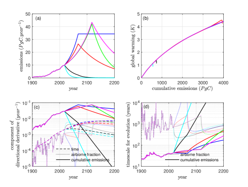
Figure 1: Conditions for path-independence between global warming and cumulative CO₂ emissions in an EBM: (a) emissions scenarios; (b) global warming versus cumulative CO₂ emissions, which is path-independent; (c) directional derivatives of global warming along axes of time, airborne fraction, and cumulative emissions; (d) timescales for evolution of airborne fraction and cumulative emissions. Global warming in the EBM is a function of cumulative emissions, airborne fraction, and time (Eq. (1)). It can be approximated as a function of cumulative emissions alone (panel b) because the directional derivative along the cumulative emissions axis is much larger (panel c). This occurs because cumulative emissions evolves on much shorter timescales (panel d).

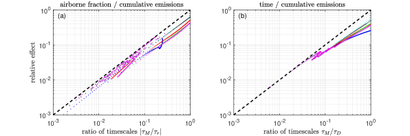
Figure 2: The effect of airborne fraction and time on global warming compared to that of cumulative emissions, as measured by their directional derivatives: (a) effect of airborne fraction relative to cumulative emissions versus the ratio of timescales for evolution of cumulative emissions and airborne fraction, illustrating Eq. (13); (b) effect of time relative to cumulative emissions versus the ratio of the cumulative emissions timescale and the damping timescale. The relative effects are bounded by the ratio of timescales, which is the main influence. For example, the relative effect of changes in the airborne fraction is small because the airborne fraction evolves slowly compared to cumulative emissions. Therefore path-independence requires $\tau_{M}/\tau_{r}$ to be small.

2.3 Model of airborne fraction with a single atmospheric time-constant

Path-independence for CO₂ with its multiple atmospheric time-constants was considered in the preceding work (Seshadri (2017b)), and the present study extends the analysis to develop a model for $\tau_{M}/\tau_{r}$ in the context of a well-mixed gas with single atmospheric time-constant $\tau$, which is relevant to many GHGs. The atmospheric cycle is described by linear differential equation

$$\frac{dC\left(t\right)}{dt}=m\left(t\right)-\frac{C\left(t\right)-C_{eq}}{\tau}$$ (16)

with emissions $m\left(t\right)$, preindustrial equilibrium concentration $C_{eq}$ at $t=0$, and atmospheric lifetime $\tau$ with which excess concentration $C\left(t\right)-C_{eq}$ is reduced. This is integrated for

$$C\left(t\right)=C_{eq}+e^{-t/\tau}\int_{0}^{t}e^{s/\tau}m\left(s\right)ds$$ (17)

Writing airborne fraction of cumulative emissions $r\left(t\right)=\left(C\left(t\right)-C_{eq}\right)/M\left(t\right)$, and differentiating

$$-\frac{1}{\tau_{r}}=\frac{1}{r}\frac{dr}{dt}=\frac{1}{C\left(t\right)-C_{eq}}\frac{d}{dt}\left(C\left(t\right)-C_{eq}\right)-\frac{1}{M\left(t\right)}\frac{d}{dt}M\left(t\right)$$ (18)

and recognizing $\tau_{M}$ in the last term on the right yields

$$\left|\frac{\tau_{M}}{\tau_{r}}\right|=\left|\frac{\tau_{M}}{C\left(t\right)-C_{eq}}\frac{d}{dt}\left(C\left(t\right)-C_{eq}\right)-1\right|$$ (19)

which must be small for path-independence.

3 Results

3.1 Path-independence is more accurate for a short-period emission cycle

Consider idealized scenarios in which emissions begin at $t=0$, reaching the maximum value at some intermediate time and subsequently declining to zero at $t=T$, where $T$ is the period of the emissions cycle (in years). Cumulative emissions during the cycle is $M\left(t\right)=\int_{0}^{t}m\left(s\right)ds$.

We introduce a dimensionless time variable $x\equiv t/T$, which ranges from $0$ to $1$. Emissions is zero at $x=0$, reaches a maximum at some $0<x<1$ and declines to zero at $x=1$. Introducing this variable separates the shape of the emissions cycle from its period. Its shape is defined by shape function $\hat{m}\left(x\right).$ A specified shape function $\hat{m}\left(x\right)$, defined over its domain from $0$ to $1,$ describes a family of emissions graphs, with $m\left(t\right)$ given by the shape function evaluated at the corresponding $x$, with $m\left(t\right)=\hat{m}\left(x\left(t\right)\right)$. Each member of the family corresponds to a different value of $T$, and fixing $T$ fixes $x\left(t\right)=t/T$ . Thus, for a given $\hat{m}\left(x\right)$ emissions cycles differ only in the value of $T.$

We shall consider the case of non-negative emissions, with $\hat{m}\left(x\right)\geq 0$ everywhere in the domain. Therefore emissions cycles with longer $T$ evolve more slowly but have larger cumulative emissions by the end of the emissions cycle. This is seen from the cumulative emissions equation

$$M\left(t\right)=\int_{0}^{t}m\left(s\right)ds$$ (20)

where $ds$ is measured in years. We rewrite in terms of $x$ by integrating between $h=0$ and $h=x$, where $dh$ is now measured in dimensionless time. In the new variable, cumulative emissions is

$$M\left(t\right)=T\int_{0}^{x\left(t\right)}\hat{m}\left(h\right)dh$$ (21)

because $ds=Tdh$. Defining a new variable analogous to cumulative emissions but with the same units as emissions

$$\hat{M}\left(x\right)\equiv\int_{0}^{x}\hat{m}\left(h\right)dh$$ (22)

which describes the integral of the emissions shape function, now without regard to period $T$ of the emissions cycle, the cumulative emissions becomes

$$M\left(t\right)=T\hat{M}\left(x\left(t\right)\right)$$ (23)

This describes the simple feature that, given a shape function $\hat{m}\left(x\right)$, cumulative emissions at corresponding positions in the cycle, for fixed $x$, scales proportionally to the emissions cycle period $T$. It is useful to examine the cumulative emissions timescale with respect to the position in the emissions cycle.

The cumulative emissions timescale, Eq. (10), becomes

$$\tau_{M}\left(t\right)=\frac{M\left(t\right)}{dM\left(t\right)/dt}=\frac{T\hat{M}\left(x\left(t\right)\right)}{T\frac{d\hat{M}\left(x\left(t\right)\right)}{dt}}$$ (24)

and, recognizing that $\frac{d\hat{M}\left(x\right)}{dt}=\frac{d\hat{M}\left(x\right)}{dx}\frac{dx}{dt}=\frac{1}{T}\frac{d\hat{M}\left(x\right)}{dx}$, and $\frac{d\hat{M}\left(x\right)}{dx}=\hat{m}\left(x\right)$ from Eq. (22), we obtain

$$\tau_{M}\left(t\right)=T\frac{\hat{M}\left(x\left(t\right)\right)}{\hat{m}\left(x\left(t\right)\right)}$$ (25)

Note that $\hat{M}\left(x\right)$ has the same units as $\hat{m}\left(x\right)$, one of the advantages in working with this form. For a given emissions shape function $\hat{m}\left(x\right)$, the cumulative emissions timescale at any time $t$ is simply $T$ times the ratio $\hat{M}\left(x\right)/$ $\hat{m}\left(x\right)$ determined at the corresponding position $x\left(t\right)=t/T$ in the emissions cycle. The cumulative emissions timescale is proportional to the emissions cycle period. Therefore path-independence, which requires a short cumulative emissions timescale compared to the airborne fraction timescale, becomes more likely for a short-period emissions cycle.

3.2 Path-independence depends on ratio $T/\tau$

Moreover, path-independence depends on the ratio $T/\tau$ between the emissions cycle period and the atmospheric lifetime. We apply the same rescaling of time as above to demonstrate this. From Eq. (17) the excess concentration at time $t$ in years is

$$C\left(t\right)-C_{eq}=e^{-t/\tau}\int_{0}^{t}e^{s/\tau}m\left(s\right)ds$$ (26)

where $ds$ describes increments of time in years. Rewriting the above integral in terms of $x$ as before,

$$\int_{0}^{t}e^{s/\tau}m\left(s\right)ds=\int_{0}^{x\left(t\right)}e^{hT/\tau}\hat{m}\left(h\right)Tdh$$ (27)

where, as before, $dh$ describes increments of dimensionless time. The above follows from $s=hT$, $ds=Tdh$, and emissions at time $s$ being determined by emissions shape function evaluated at corresponding $h$, i.e. $m\left(s\right)=\hat{m}\left(h\left(s\right)\right)$. Hence we can rewrite, for excess concentration at $x=t/T$

$$C\left(x\left(t\right)\right)-C_{eq}=Te^{-\alpha x\left(t\right)}\int_{0}^{x\left(t\right)}e^{\alpha h}\hat{m}\left(h\right)dh$$ (28)

where $\alpha=T/\tau$. Very simply, we have rewritten $t/\tau$ appearing in Eq. (26) as $\left(T/\tau\right)\left(t/T\right)=\alpha x$, with the extra $T$ arising from change in integration variable from $t$ (measured in years) to $x$ (measured in dimensionless time).

Rewriting the excess concentration in terms of the emissions shape function and the emissions cycle period illuminates the problem’s structure. Integrating by parts,

$$e^{-\alpha x}\int_{0}^{x}e^{\alpha h}\hat{m}\left(h\right)dh=\hat{m}_{1}\left(x\right)-\alpha\hat{m}_{2}\left(x\right)+\alpha^{2}\hat{m}_{3}\left(x\right)-\ldots$$ (29)

where $\hat{m}_{i}\left(x\right)=\intop_{0}^{x}\hat{m}_{i-1}\left(h\right)dh$ is the $i$^th repeated integral of emissions having the same units as $\hat{m}\left(x\right)$, and we define $\hat{m}_{0}\left(x\right)\equiv\hat{m}\left(x\right)$. Then $\hat{M}\left(x\right)$, the integral of the emissions shape function, becomes $\hat{m}_{1}\left(x\right)$. From Eqs. (19)-(28) we obtain the ratio

$$\left|\frac{\tau_{M}}{\tau_{r}}\right|=\left|\frac{1-\alpha\frac{\hat{m}_{1}\left(x\right)}{\hat{m}\left(x\right)}+\alpha^{2}\frac{\hat{m}_{2}\left(x\right)}{\hat{m}\left(x\right)}-\ldots}{1-\alpha\frac{\hat{m}_{2}\left(x\right)}{\hat{m}_{1}\left(x\right)}+\alpha^{2}\frac{\hat{m}_{3}\left(x\right)}{\hat{m}_{1}\left(x\right)}-\ldots}-1\right|$$ (30)

which must be small for path-independence as shown above. This condition depends on integrals of the emissions shape function and the value of dimensionless parameter $\alpha=T/\tau$. For fixed position in the emissions cycle, i.e. given $x$, accuracy of the path-independence approximation depends on $\alpha$. In the limit $\alpha\rightarrow 0$, $\left|\frac{\tau_{M}}{\tau_{r}}\right|\rightarrow 0$ and path-independence obviously holds. This is roughly the case of very long atmospheric lifetime, as compared to the period of the emissions cycle.

3.3 Condition for path-independence

In general $\alpha$ is not necessarily close to zero, even for long-lived GHGs, but the ratio in Eq. (30) might be small enough that path-independence is a reasonable approximation. This ratio depends on $\alpha$ and $x$ alone, once the shape function $\hat{m}\left(x\right)$ is specified. Generally the shape function may be arbitrary, but for clarity we consider stylized scenarios of the form $\hat{m}\left(x\right)=\beta x^{\gamma}$ during the increasing phase of emissions between $0\leq x<\frac{1}{2}$, and for the decreasing phase during $\frac{1}{2}\leq x\leq 1$, $\hat{m}\left(x\right)=\beta\left(1-x\right)^{\gamma}$, a mirror-image. We have assumed $\beta>0$ and $\gamma>0$. Emissions peaks at $x=\frac{1}{2}$ and declines to zero at $x=1$. We recall that once the shape function is specified, we must additionally know the emissions cycle period $T$ to know the emissions profile in time.

This form of the emissions shape function renders Eq. (30) as a series in $\alpha x$, illuminating the structure of the problem. During the increasing phase of emissions, repeated integrals are related as $\hat{m}_{i}\left(x\right)/\hat{m}\left(x\right)=x^{i}/\left\{\left(\gamma+1\right)\left(\gamma+2\right)\ldots\left(\gamma+i\right)\right\}$ and $\hat{m}_{i+1}\left(x\right)/\hat{m_{1}}\left(x\right)=x^{i}/\left\{\left(\gamma+2\right)\left(\gamma+3\right)\ldots\left(\gamma+i+1\right)\right\}$ . These terms, appearing in Eq. (30), with increasing powers of $x<\frac{1}{2}$ and growing factorial-like terms in the denominator, rapidly decline with $i$. Even for the decreasing phase where $\frac{1}{2}\leq x\leq 1$, these terms decline rapidly and the series converges (as shown in Supplementary Information, SI).

For concreteness we consider the increasing phase of emissions, and stipulate a tolerance $\theta\ll 1$ on the accuracy of path-independence, setting down that path-independence would be an adequate approximation if $\left|\frac{\tau_{M}}{\tau_{r}}\right|\leq\theta$. In general the error from neglecting the contributions to the directional derivative along the axis of $r$ should be quite small, typically much lesser than 1, for the path independence approximation to be valid. This requires that in Eq. (13), the product $\theta R_{r}\ll 1$. If we had $R_{r}\ll 1$, then $\theta$ would not have to be especially small. In general, this is not the case, as seen in Figure 2, and we assume that $\theta$ must be small enough to carry the burden of limiting the quantity in Eq. (13).

Then the condition for path-independence $0\leq\left|\frac{\tau_{M}}{\tau_{r}}\right|\leq\theta\ll 1$ becomes

$$\left|\left\{1-\alpha\frac{\hat{m}_{1}\left(x\right)}{\hat{m}\left(x\right)}+\alpha^{2}\frac{\hat{m}_{2}\left(x\right)}{\hat{m}\left(x\right)}-\ldots\right\}-\left\{1-\alpha\frac{\hat{m}_{2}\left(x\right)}{\hat{m}_{1}\left(x\right)}+\alpha^{2}\frac{\hat{m}_{3}\left(x\right)}{\hat{m}_{1}\left(x\right)}-\ldots\right\}\right|\\ \leq\theta\left|\left\{1-\alpha\frac{\hat{m}_{2}\left(x\right)}{\hat{m}_{1}\left(x\right)}+\alpha^{2}\frac{\hat{m}_{3}\left(x\right)}{\hat{m}_{1}\left(x\right)}-\ldots\right\}\right|$$ (31)

and, truncating up to $\alpha^{3}$ and defining a new dimensionless variable $y\equiv\alpha x=t/\tau$, we obtain the condition in terms of the following inequality in cubic polynomial in $y$

$$g\left(y\right)=\left\{3+\theta\left(\gamma+1\right)\right\}y^{3}-\left\{2+\theta\left(\gamma+1\right)\right\}\left(\gamma+4\right)y^{2}+\left\{1+\theta\left(\gamma+1\right)\right\}\left(\gamma+3\right)\left(\gamma+4\right)y\\ -\theta\left(\gamma+1\right)\left(\gamma+2\right)\left(\gamma+3\right)\left(\gamma+4\right)\leq 0$$ (32)

which is increasing everywhere (please see SI). Furthermore, $g(0)<0$ so that it has positive root $y^{*}$ where $g\left(y^{*}\right)=0$. This root depends on $\theta$ and $\gamma$. Characterizing the solutions to this cubic equation is important, and its graph in Figure 3 illustrates the aforementioned properties.The mathematics of path-independence reduces to solving this family of cubic polynomials possessing a single root. The approach illustrates simultaneously three features of the path independence problem: path independence depends on the value of $y\equiv\alpha x$, whose effect can in turn be decomposed into the position in the emissions cycle and the parameter $\alpha$, and depends on the curvature of the emissions shape function through $\gamma$.

Path-independence with tolerance $\theta$ requires $y<y^{*}\left(\theta,\gamma\right)$, or $t<\tau y^{*}\left(\theta,\gamma\right)$, and occurs more easily earlier in the emissions cycle. For example, path-independence is a valid approximation around the time of the emissions peak at $t=T/2$ if the period of the emissions cycle $T<2\tau y^{*}\left(\theta,\gamma\right)$ and $3/4$^th into the emissions cycle if $T<\frac{4}{3}\tau y^{*}\left(\theta,\gamma\right)$, imposing a progressively more stringent condition further into the cycle. This is because the cumulative emissions timescale grows with the position in the cycle, with its value being $\tau_{M}=Tx/\left(\gamma+1\right)$ during the increasing phase of emissions, and a corresponding expression increasing in $x$ for the decreasing phase of emissions (the latter is discussed in SI). Symbols used in this section to describe path independence are listed in Table 3.

Table 3: Symbols used in describing path independence

Symbol	Description	Units
$\tau_{M}$	cumulative emissions timescale	years
$\tau_{r}$	airborne fraction timescale	years
$t$	time	years
$x$	rescaled time	dimensionless
$\hat{m}\left(x\right)$	emissions shape function	same as $m\left(t\right)$
$\hat{M}\left(x\right)$	integral of emissions shape function	same as $\hat{m}\left(x\right)$
$\hat{m_{i}}\left(x\right)$	$i$th repeated integral of $\hat{m}\left(x\right)$	same as $\hat{m}\left(x\right)$
$\tau$	atmospheric lifetime	years
$T$	emissions cycle period	years
$\alpha$	ratio of $T/\tau$	dimensionless
$y$	product $\alpha x=t/\tau$	dimensionless
$y^{*}$	root of condition $g\left(y\right)<0$ for path independence	dimensionless
$\gamma$	exponent of emissions shape function	dimensionless
$\theta$	tolerance on path-independence accuracy	dimensionless

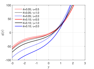
Figure 3: Graph of cubic polynomial in Eq. (32). The function is increasing in $y$, takes a negative value at $y=0$, and has a single positive root that lies between $0$ and $1$ for parameter values considered here.

In addition to the emissions shape function, it has been assumed that the 3^rd-order truncation of the series in Eq. (30) is adequate. This is justified in Figure 4, which shows contours of $\theta$ as a function of $x$ and $\alpha$. Owing to the inequality constraint, path-independence occurs to the lower left side of the contours. Shown are the exact values, corresponding to the ratio $\left|\frac{\tau_{M}}{\tau_{r}}\right|$ in Eq. (19), and 1^st- 3^rd order approximations. The approximation to 3^rd order in $y$ has converged and, since path-independence involves a constraint on $y=\alpha x$, the resulting boundaries are families of hyperbolas.

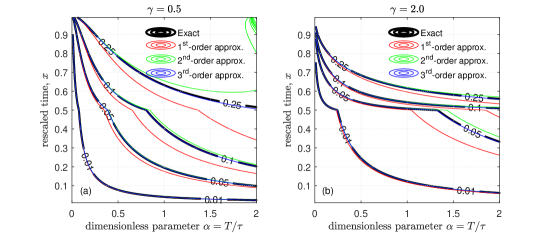
Figure 4: Contour plot of tolerance $\theta$ versus the dimensionless parameter $\alpha=T/\tau$ and rescaled time $x=t/T$. Black lines show exact values from numerical integration of Eq. (19) whereas colors show successive series approximations involving Eq. (31). The cubic approximation performs well for a wide range of the emissions parameter $\gamma$ and conditions in $\alpha$ and $x$. Therefore Eq. (32) is an adequate account of path-independence. This equation provides an inequality constraint on $y=\alpha x$ and the corresponding boundaries in the figure are hyperbolas. Path-independence occurs if $\alpha=T/\tau$ is equal to or smaller than the corresponding contour line. Further into the emissions cycle, measured by higher $x$, the condition for path-independence becomes more stringent, requiring smaller $\alpha$. For a more sharply peaked emissions cycle, involving higher $\gamma,$ the condition for path-independence becomes less stringent, entailing a rightward shift in the boundaries towards higher $\alpha$.

The shape function, as characterized by $\gamma$, has an important effect. The cumulative emissions timescale during the increasing phase is $\tau_{M}=Tx/\left(\gamma+1\right)$ as noted earlier, which is short for small $T$ or large $\gamma$. This is also true of the decreasing phase (please refer to SI). Hence more sharply-peaked emissions graphs, with higher $\gamma$, can lead to shorter cumulative emissions timescales and satisfy path-independence to a better approximation. The main influence remains of course the period of the emissions cycle. These results are summarized in Figure 5, which shows that the ratio of timescales $\left|\frac{\tau_{M}}{\tau_{r}}\right|$ is a function of $\alpha=T/\tau$. The figure also depicts the range of validity of the cubic approximation, which fails for higher $\alpha$.

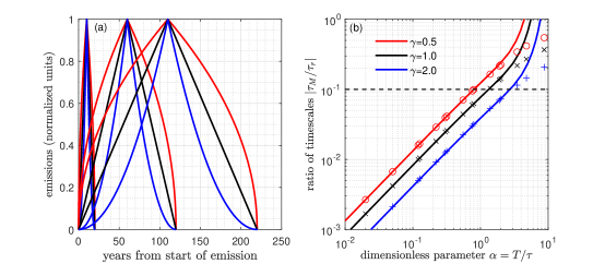
Figure 5: The ratio of timescales $\left|\tau_{M}/\tau_{r}\right|$ at the peak of the emissions graph, i.e. $x=\frac{1}{2}$, as a function of the dimensionless parameter $\alpha=T/\tau$ and the sharpness of the emissions shape function, as measured by exponent $\gamma$. This is drawn for different emissions graphs depicted in the left panel. On the right panel, markers describe exact values from Eq. (19), whereas the continuous lines show approximations from the model of Eq. (30) truncated to cubic terms. The model is valid for small ratio of timescales, including where $\left|\tau_{M}/\tau_{r}\right|\leq 0.1$ for which it is stipulated that path-independence holds. This value of $\left|\tau_{M}/\tau_{r}\right|$ is governed by the ratio between the period of the emissions cycle and the atmospheric lifetime. For example, with $\gamma$ between $0.5$ and $1.0$, the ratio $\left|\tau_{M}/\tau_{r}\right|<0.1$ at the emissions peak if, approximately, $T\leq\tau$. For a given atmospheric lifetime, this entails a short emissions cycle. For a more sharply peaked emissions cycle with higher $\gamma,$ path-independence can occur for larger $T$, corresponding to families of emissions cycles having longer periods.

3.4 Example

The above account of path-independence has practical relevance even to those GHGs with lifetime considerably shorter than CO₂, whose emissions have recently begun. A good example is hydrofluorocarbons (HFC) that replaced ozone-depleting substances under the implementation of the Montreal Protocol, with their emissions beginning to grow during the early 1990s (Velders et al. (2009); Lunt et al. (2015); Stanley et al. (2020)). These HFCs are greenhouse gases with large global warming potentials, and individual lifetimes ranging from few years to a few hundred years (Naik et al. (2000)). Their present contribution to radiative forcing is quite small, but projected to increase by two orders of magnitude by end of century, to larger than 0.1 W m^-2, if unabated (Velders et al. (2009); Zhang et al. (2011); Velders et al. (2015)). In the future some important contributors are expected to include HFC22 (12), HFC134a (14), HFC125 (29), HFC152a (1.4), HFC143a (52), and HFC32 (4.9), with estimated lifetimes (in years) listed in brackets (Naik et al. (2000); Zhang et al. (2011)).

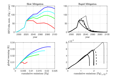
Figure 6: Global warming versus cumulative emissions for HFC143a, with atmospheric lifetime of 52 years. Left-side panels show scenarios involving slow mitigation, whereas right-side panels show rapid mitigation. Each color in the left-side panels shows a different emissions scenario, and each linestyle in the right-side panels shows a different scenario. Global warming is independent of emissions pathway if the emissions cycles play out over timescales comparable to the atmospheric lifetime (right-side panels).

The example of HFC143a (Figure 6) is particularly relevant, because its lifetime of 52 years is still longer than the roughly 30-year period that has elapsed since its emissions began (Orkin et al. (1996); Zhang et al. (2011)). Past annual emissions are drawn from Simmonds et al. (2017), for the period 1991-2015. During the years 2016 to 2019, we interpolate the RCP3 scenario (van Vuuren et al. (2007); Meinshausen et al. (2011)) and future scenarios in the left panels are modification of the basic RCP3 scenario, with both larger and smaller emissions scenarios included (Figure 6a). Radiative forcing of HFC143a is linear in concentrations (in ppbv) (Naik et al. (2000); Zhang et al. (2011); Stocker et al. (2013)). Global warming is computed for HFC143a from numerical integrations of the 2-box EBM (Held et al. (2010)). The lower-left panel (c) shows that cumulative emissions accounting is not applicable for these scenarios because the relation between global warming and cumulative emissions is not path-independent. The right panel (Figure 6b) presents scenarios involving much more rapid mitigation, so that emissions decrease to nearly zero by the middle of the 21^st century. For these scenarios, during the growing phase of cumulative emissions of HFC143a while annual emissions are non-zero, global warming is approximately a function of cumulative emissions. This breaks down only after cumulative emissions stop growing and the global warming contribution begins to decrease following a draw-down of concentrations, as also occurs for CO₂. During the increasing phase of cumulative emissions, path-independence is a good approximation, supporting cumulative emissions accounting for such a scenario family.

4 Discussion

Path-independence of the relation between global warming and cumulative emissions is adequate for cumulative emissions accounting, and hence its mathematics bears examination. The question of path-independence is whether global warming can be approximated by cumulative emissions alone, and this occurs where directional derivatives of global warming with respect to the other parameters are small compared to the effect of cumulative emissions. The idealized account of this paper, based on an explicit formula for global warming obtained by integrating an EBM (Seshadri (2017a)), shows that no special model of radiative forcing or atmospheric cycle is necessary. Path-independence only requires the emissions cycle to progress rapidly enough that the cumulative emissions timescale is short compared to the timescale for evolution of the airborne fraction. This broadens the potential relevance of cumulative emissions accounting beyond CO₂, especially to other GHGs with lifetimes of several decades whose emissions have recently begun.

The cumulative emissions timescale depends on the period of the emissions cycle and its shape, but not its amplitude. Quantitatively, if the emissions cycle proceeds with a period comparable to or less than the atmospheric lifetime, path-independence is approximately valid, because the effects of changes in airborne fraction are an order of magnitude smaller than the effect of growing cumulative emissions. In effect, if the emissions cycle is rapid compared to the atmospheric lifetime, it does not matter when the species is emitted.

For GHGs with lifetime on the range of several decades, this could occur if the emissions cycle proceeds rapidly enough. This has been illustrated for HFC143a. Although this has a much shorter atmospheric lifetime than CO₂ of about 52 years, since its emissions began only in the 1990s (Simmonds et al. (2017)), cumulative emissions accounting would be applicable to this species while considering scenarios where the emissions were to be reduced substantially if not eliminated during the first half of the 21^st century. Of course, this is not relevant to the much shorter-lived HFCs, or to short-lived climate pollutants in general.

Path-independence is a straightforward result of differing timescales, and does not depend on particular physics of climate forcers or the Earth system. The present model considers only single atmospheric time-constants, but can be readily extended to multiple time-constants or baskets of greenhouse gases such as the HFCs considered together (Velders et al. (2009, 2015)). It makes predictions that would be useful to examine using more complex models. Sharply-peaked emissions cycles present rapid evolution of cumulative emissions, with shorter cumulative emissions timescales, so path-independence can occur somewhat more easily in this case. The adequacy of the path-independence approximation degrades with progression of the emissions cycle, owing to increase in the cumulative emissions timescale with time. These are made explicit using the power-law model of the emissions cycle, but the qualitative conclusions are broadly applicable and observed in the results involving the more general emissions scenarios presented here.

References

- Allen et al. (2009) Allen, M. R., D. J. Frame, C. Huntingford, C. D. Jones, J. A. Lowe, M. Meinshausen, and N. Meinshausen (2009), Warming caused by cumulative carbon emissions towards the trillionth tonne, Nature, 458, 1163–1166, doi:http://dx.doi.org/10.1038/nature08019.
- Allen et al. (2016) Allen, M. R., J. S. Fuglestvedt, K. P. Shine, A. Reisinger, R. T. Pierrehumbert, and P. M. Forster (2016), New use of global warming potentials to compare cumulative and short-lived climate pollutants, Nature Climate Change, 6, 773–777, doi:10.1038/NCLIMATE2998.
- Bowerman et al. (2011) Bowerman, N. H. A., D. J. Frame, C. Huntingford, J. A. Lowe, and M. R. Allen (2011), Cumulative carbon emissions, emissions floors and short-term rates of warming: implications for policy, Philosophical Transactions of the Royal Society of London A, 369, 45–66, doi:http://dx.doi.org/10.1098/rsta.2010.0288.
- Frame et al. (2019) Frame, D. J., L. J. Harrington, J. S. Fuglestvedt, R. J. Millar, M. M. Joshi, and S. Caney (2019), Emissions and emergence: a new index comparing relative contributions to climate change with relative climatic consequences, Environmental Research Letters, 14, 1–10, doi:10.1088/1748-9326/ab27fc.
- Friedlingstein et al. (2019) Friedlingstein, P., M. W. Jones, M. O’Sullivan, R. M. Andrew, J. Hauck, and G. P. Peters (2019), Global Carbon Budget 2019, Earth System Science Data, 11, 1783–1838, doi:10.5194/essd-11-1783-2019.
- Fuglestvedt et al. (2003) Fuglestvedt, J. S., T. K. Berntsen, O. Godal, R. Sausen, K. P. Shine, and T. Skodvin (2003), Metrics of climate change: assessing radiative forcing and emission indices, Climatic Change, 58, 267–331, doi:10.1023/A:1023905326842.
- Geoffroy et al. (2013a) Geoffroy, O., D. Saint-Martin, D. J. L. Olivie, A. Voldoire, G. Bellon, and S. Tyteca (2013a), Transient climate response in a two-layer energy-balance model: Part 1: analytical solution and parameter calibration using CMIP5 AOGCM experiments, Journal of Climate, 26, 1841–1857, doi:http://dx.doi.org/10.1175/JCLI-D-12-00195.1.
- Geoffroy et al. (2013b) Geoffroy, O., D. Saint-Martin, G. Bellon, A. Voldoire, D. J. L. Olivie, and S. Tyteca (2013b), Transient climate response in a two-layer energy-balance model. Part II: Representation of the efficacy of deep-ocean heat uptake and validation for CMIP5 AOGCMs, Journal of Climate, 26, 1859–1876, doi:http://dx.doi.org/10.1175/JCLI-D-12-00196.1.
- Goodwin et al. (2015) Goodwin, P., R. G. Williams, and A. Ridgwell (2015), Sensitivity of climate to cumulative carbon emissions due to compensation of ocean heat and carbon uptake, Nature Geoscience, 8, 29–34, doi:http://dx.doi.org/10.1038/ngeo2304.
- Gregory (2000) Gregory, J. M. (2000), Vertical heat transports in the ocean and their effect on time-dependent climate change, Climate Dynamics, 16, 501–515, doi:http://dx.doi.org/10.1007/s003820000059.
- Hall et al. (2019) Hall, A., P. Cox, C. Huntingford, and S. Klein (2019), Progressing emergent constraints on future climate change, Nature Climate Change, 9, 269–278, doi:10.1038/s41558-019-0436-6.
- Held et al. (2010) Held, I. M., M. Winton, K. Takahashi, T. Delworth, F. Zeng, and G. K. Vallis (2010), Probing the fast and slow components of global warming by returning abruptly to preindustrial forcing, Journal of Climate, 23, 2418–2427, doi:http://dx.doi.org/10.1175/2009JCLI3466.1.
- Herrington and Zickfeld (2014) Herrington, T., and K. Zickfeld (2014), Path independence of climate and carbon cycle response over a broad range of cumulative carbon emissions, Earth System Dynamics, 5, 409–422, doi:http://dx.doi.org/10.5194/esd-5-409-2014.
- Lunt et al. (2015) Lunt, M. F., M. Rigby, A. L. Ganesan, A. J. Manning, R. G. Prinn, and S. O’Doherty (2015), Reconciling reported and unreported HFC emissions with atmospheric observations, Proceedings of the National Academy of Sciences, 112, 5927–5931, doi:10.1073/pnas.1420247112.
- MacDougall and Friedlingstein (2015) MacDougall, A. H., and P. Friedlingstein (2015), The origin and limits of the near proportionality between climate warming and cumulative CO2 emissions, Journal of Climate, 28, 4217–4230, doi:http://dx.doi.org/10.1175/JCLI-D-14-00036.1.
- Matthews et al. (2009) Matthews, H. D., N. P. Gillett, P. A. Stott, and K. Zickfeld (2009), The proportionality of global warming to cumulative carbon emissions, Nature, 459, 829–832, doi:http://dx.doi.org/10.1038/nature08047.
- Matthews et al. (2012) Matthews, H. D., S. Solomon, and R. T. Pierrehumbert (2012), Cumulative carbon as a policy framework for achieving climate stabilization, Philosophical Transactions of the Royal Society of London A, 370, 4365–4379, doi:http://dx.doi.org/10.1098/rsta.2012.0064.
- Meinshausen et al. (2009) Meinshausen, M., N. Meinshausen, W. Hare, S. C. B. Raper, K. Frieler, R. Knutti, D. J. Frame, and M. R. Allen (2009), Greenhouse-gas emission targets for limiting global warming to 2C, Nature (London, United Kingdom), 458, 1158–1162, doi:10.1038/nature08017.
- Meinshausen et al. (2011) Meinshausen, M., S. J. Smith, K. Calvin, J. S. Daniel, and M. L. T. Kainuma (2011), The RCP greenhouse gas concentrations and their extensions from 1765 to 2300, Climatic Change, 109, 213–241, doi:http://dx.doi.org/10.1007/s10584-011-0156-z.
- Millar et al. (2017) Millar, R. J., J. S. Fuglestvedt, P. Friedlingstein, M. Grubb, J., Rogelj, and H. D. Matthews (2017), Emission budgets and pathways consistent with limiting warming to 1.5°C, Nature Geoscience, 10, 741–747, doi:10.1038/ngeo3031.
- Naik et al. (2000) Naik, V., A. K. Jain, K. O. Patten, and D. J. Wuebbles (2000), Consistent sets of atmospheric lifetimes and radiative forcings on climate for CFC replacements: HCFCs and HFCs, Journal of Geophysical Research, 105, 6903–6914, doi:10.1029/1999JD901128.
- Nijsse et al. (2020) Nijsse, F. J., P. M. Cox, and M. S. Williamson (2020), An emergent constraint on Transient Climate Response from simulated historical warming in CMIP6 models, Earth System Dynamics Discussions, pp. 1–14, doi:10.5194/esd-2019-86.
- Orkin et al. (1996) Orkin, V. L., R. E. Huie, and M. J. Kurylo (1996), Atmospheric Lifetimes of HFC-143a and HFC-245fa: Flash Photolysis Resonance Fluorescence Measurements of the OH Reaction Rate Constants, The Journal of Physical Chemistry, 100, 8907–8912, doi:10.1021/jp9601882.
- Seshadri (2017a) Seshadri, A. K. (2017a), Fast-slow climate dynamics and peak global warming, Climate Dynamics, 48, 2235–2253, doi:10.1007/s00382-016-3202-8.
- Seshadri (2017b) Seshadri, A. K. (2017b), Origin of path independence between cumulative CO2 emissions and global warming, Climate Dynamics, 49, 3383–3401, doi:10.1007/s00382-016-3519-3.
- Shine et al. (2005) Shine, K., J. S. Fuglestvedt, K. Hailemariam, and N. Stuber (2005), Alternatives to the global warming potential for comparing climate impacts of emissions of greenhouse gases, Climatic Change, 68, 281–302, doi:10.1007/s10584-005-1146-9.
- Simmonds et al. (2017) Simmonds, P. G., M. Rigby, A. McCulloch, S. O’Doherty, D. Young, and J. Muhle (2017), Changing trends and emissions of hydrochlorofluorocarbons (HCFCs) and their hydrofluorocarbon (HFCs) replacements, Atmospheric Chemistry and Physics, 17, 4641–4655, doi:10.5194/acp-17-4641-2017.
- Stanley et al. (2020) Stanley, K., D. Say, J. Muhle, C. Harth, P. Krummel, D. Young, and S. O’Doherty (2020), Increase in global emissions of HFC-23 despite near-total expected reductions, Nature Communications, 396, 1–6, doi:10.1038/s41467-019-13899-4.
- Stocker (2013) Stocker, T. F. (2013), The closing door of climate targets, Science, 339, 280–282, doi:http://dx.doi.org/10.1126/science.1232468.
- Stocker et al. (2013) Stocker, T. F., D. Qin, G.-K. Plattner, L. V. Alexander, and S. K. Allen (2013), Climate Change 2013: The Physical Science Basis. Contribution of Working Group I to the Fifth Assessment Report of the Intergovernmental Panel on Climate Change, chap. Technical Summary, pp. 33–118, Cambridge University Press.
- Stouffer (2004) Stouffer, R. J. (2004), Time scales of climate response, Journal of Climate, 17, 209–217, doi:http://dx.doi.org/10.1175/1520-0442(2004)017<0209:TSOCR>2.0.CO;2.
- van Vuuren et al. (2007) van Vuuren, D. P., M. G. J. den Elzen, P. L. Lucas, B. Eickhout, and B. J. Strengers (2007), Stabilizing greenhouse gas concentrations at low levels: an assessment of reduction strategies and costs, Climatic Change, 81, 119–159, doi:10.1007/s10584-006-9172-9.
- Velders et al. (2015) Velders, G. J., D. W. Fahey, J. S. Daniel, S. O. Andersen, and M. McFarland (2015), Future atmospheric abundances and climate forcings from scenarios of global and regional hydrofluorocarbon (HFC) emissions, Atmospheric Environment, 123, 200–209, doi:10.1016/j.atmosenv.2015.10.071.
- Velders et al. (2009) Velders, G. J. M., D. W. Fahey, J. S. Daniel, M. McFarland, and S. O. Andersen (2009), The large contribution of projected HFC emissions to future climate forcing, Proceedings of the National Academy of Sciences, 106, 10,949–10,954, doi:10.1073/pnas.0902817106.
- Winton et al. (2010) Winton, M., K. Takahashi, and I. M. Held (2010), Importance of ocean heat uptake efficacy to transient climate change, Journal of Climate, 23, 2333–2344, doi:http://dx.doi.org/10.1175/2009JCLI3139.1.
- Zhang et al. (2011) Zhang, H., J. Wu, and P. Lu (2011), A study of the radiative forcing and global warming potentials of hydrofluorocarbons, Journal of Quantitative Spectroscopy & Radiative Transfer, 112, 220–229, doi:10.1016/j.jqsrt.2010.05.012.
- Zickfeld et al. (2009) Zickfeld, K., M. Eby, H. D. Matthews, and A. J. Weaver (2009), Setting cumulative emissions targets to reduce the risk of dangerous climate change, Proceedings of the National Academy of Sciences of the United States of America, 106, 16,129–16,134, doi:http://dx.doi.org/10.1073/pnas.0805800106.
- Zickfeld et al. (2012) Zickfeld, K., V. K. Arora, and N. P. Gillett (2012), Is the climate response to carbon emissions path dependent?, Geophysical Research Letters, 39, 1–6, doi:10.1029/2011GL050205.