subfig
Modeling and Control of a Hybrid Wheeled Jumping Robot
Abstract
In this paper, we study a wheeled robot with a prismatic extension joint. This allows the robot to build up momentum to perform jumps over obstacles and to swing up to the upright position after the loss of balance. We propose a template model for the class of such two-wheeled jumping robots. This model can be considered as the simplest wheeled-legged system. We provide an analytical derivation of the system dynamics which we use inside a model predictive controller (MPC). We study the behavior of the model and demonstrate highly dynamic motions such as swing-up and jumping. Furthermore, these motions are discovered through optimization from first principles. We evaluate the controller on a variety of tasks and uneven terrains in a simulator.
I Introduction
Wheels have been used by humanity since the Bronze age. Wheeled vehicles have enabled fast and reliable transport of goods across great distances due to their simplicity and efficiency. However, they require structured terrain such as roads or rails. Legged robots on the other hand are capable of navigating unstructured, rough terrain, including jumping over obstacles and across gaps. This comes at the cost of a more complex mechanical structure. This complexity makes the robot more expensive to control—both in terms of computation as well as energy expenditure. Wheel-legged robots can combine the best of both designs—the fast motion of a wheeled system with the ability to navigate rugged terrain via legged locomotion.
For model-based control, a model of the system is needed. It should be able to handle the rolling contact of the wheels as well as the discrete contact changes typical for stepping and jumping motions of legged robots. However, instead of adding complexity to a legged robot model by adding the rolling contact, we choose to focus on developing a simplified model with only one prismatic joint to ‘mimic’ the capability of a leg. This provides us with a better tool for modeling the robot behavior than some of the more complex models.
https://youtu.be/j2sIWL8m2pQ
Most wheel-legged robots ([1, 2, 3, 4, 5]) are high degree of freedom nonlinear systems which do not lend themselves readily to online whole-body trajectory optimization (TO).
Previous work [6, 5, 7] explored kinematic motion planning where the robot is controlled like a mobile vehicle and the legs act as a suspension. By definition, these techniques do not consider the dynamics of the system.
The authors of [1] use a linear quadratic regulator (LQR) for balancing the Ascento robot. They linearize the nonlinear system dynamics around the fixed point at the upright configuration. This provides an efficient approximation but it limits the range of motion around the fixed point [8, Chapter 3].
By contrast, ANYmal [2] uses a centroidal dynamics model [9] in a two-stage controller: One for the center of mass (CoM) and one for the wheels. This approach, therefore, fails to exploit potential combined synergies of the wheel and body dynamics.
Skaterbots [4] solve the full optimization. However, due to the complexity of the resulting nonlinear program, the constraints are expressed as cost terms and optimized using Newton’s method. Compared to Skaterbots, we are able to solve the nonlinear problem due to the simple template model. Additionally, here, we use a Model Predictive Controller scheme, compared to the PD control used in Skaterbots.
Finally, the authors in [10] propose a Quadratic Programming (QP)-based approach to wheel-legged locomotion. In order to make the problem tractable, the -component of the trajectory, as well as the CoM trajectory are taken as inputs to the QP-solver. In contrast, we directly optimize the -component of the robot, thus allowing the optimizer to discover jump-like motions.
The Handle and the Flea by Boston Dynamics show remarkably dynamic motions. Flea is capable of jumping to a height of using combustive propulsion [11]. Handle shows jumping motion while driving forward, as well as traversing rugged terrain. However, methods used to control these systems have not been published.
Indeed, there is a gap with respect to the control of wheel-legged robots. Staged optimization and linearization schemes inherently do not allow for the system to fully exploit its dynamics. Motions such as jumping are hard to execute using these schemes. Jumping in particular is often accomplished using a hand-tuned controller (e.g. Ascento [1] and AirHopper [12]).
Instead of considering the full rigid body dynamics, one can model the system using simpler template models that capture the essence of the robot dynamics.
A popular template model for legged robots is the Spring-Loaded Inverted Pendulum (SLIP) [13]. SLIP has been used for high speed running and jumping [14]. For wheeled balancing systems, Wheeled Inverted Pendulum models (WIP) have been extensively used as template models [15]. Template models based on SLIP and WIP can be applied to wheel-legged systems, however they will consider either only the leg or only the wheel, respectively.
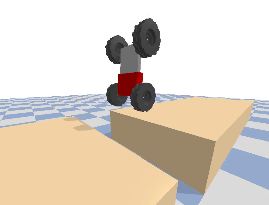
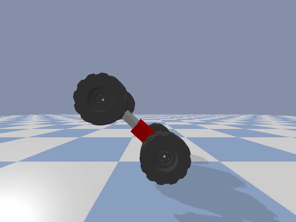
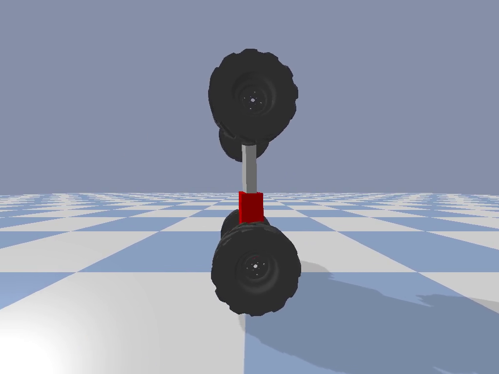
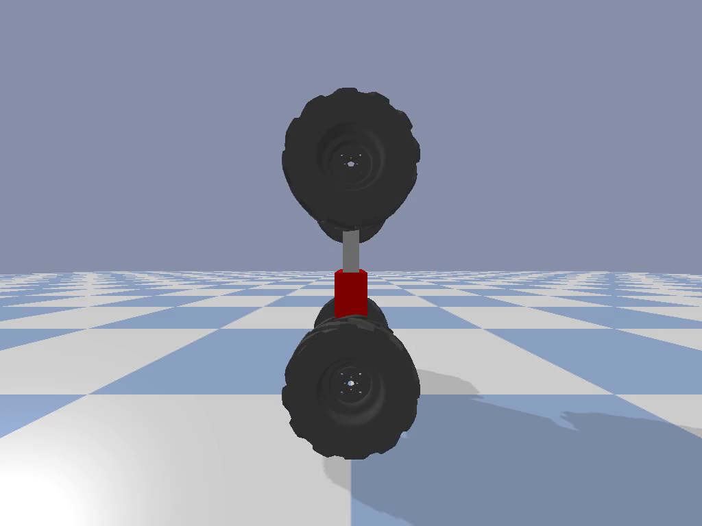
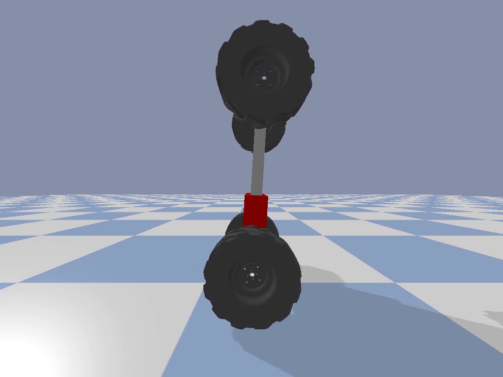
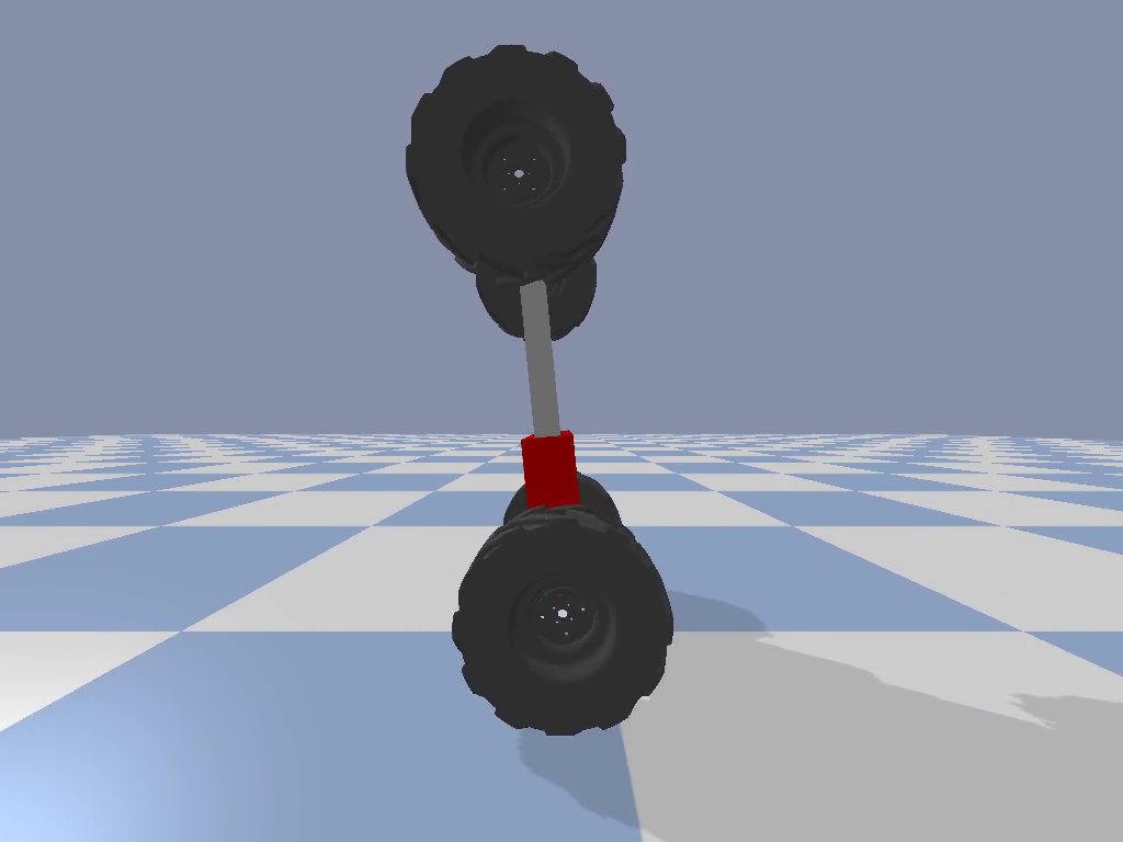
In this paper, we propose the simplest template model of wheel-legged robots. Our system consists of two sets of wheels connected by a prismatic joint (see Figure 1). Our main contributions are:
-
•
We propose the Variable-Length Wheeled Inverted Pendulum (VL-WIP) template model for wheeled-legged systems.
-
•
We implement a motion planner using the VL-WIP model and the direct transcription method which we integrate into a Model Predictive Controller (MPC).
-
•
We show that using the VL-WIP model, the robot can execute motions such as jumping that are only achievable using the combined action of wheels and base.
-
•
We validate the controller in a closed loop in a physics simulator, and we evaluate the robustness of the MPC with sensor noise and on a rough terrain locomotion task. We also compare these results to a Proportional Derivative (PD) controller on a driving and balancing task.
The ability to discover dynamic motion and to exploit the predictive power of the controller stems from the dynamics model we propose.
II Dynamics Model
We begin by modeling the system behavior using a template model we call a Variable-Length Wheeled Inverted Pendulum (VL-WIP). Our model is based on the WIP model which is used to control balancing robots [15]. WIP consists of a wheel and a pole. The pole is modeled as a point mass a fixed distance away from the wheel (see the derivation in [16]). We extend this model to include a prismatic joint and a floating base described by a -coordinate as shown in Figure 2.
The dynamics model describes the system behavior in terms of its state and controls , where is the generalized position and is the generalized velocity. The generalized position is , where are the coordinates of the center of the wheel, is the wheel’s angle along its axis, is the distance from the center of the wheel to the body point mass and is the rotation of the body from the inertia -axis. Controls are , where is actuation torque of the wheel and is the linear force in the prismatic joint. The explicit Equations of Motion (EoM) for the system under contact can be written as:
| (1) |
where is the mass matrix, is the Coriolis matrix, is the gravity vector, is a selection matrix, is the contact Jacobian and stands for the contact forces. Note that, this dynamics equation also applies when the robot is in flight and the contact forces vanish. We compute , and using Lagrangian dynamics. For the full derivation, see the Appendix. The results of this derivation are the following matrices:
| (2) | ||||
| (3) | ||||
| (4) |
where is the total mass which sums up the body mass and the wheel mass , is the inertia of the wheel, and .
The matrix translates controls and into the generalized coordinates of the system. directly maps to the prismatic joint. The torque applied on the wheel will lead to a counter reaction torque on the body of the robot. We write this down as:
| (5) |
Finally, the contact Jacobian relates the velocity of the contact point to the generalized velocities of the robot:
| (6) |
where is the radius of the wheel.
Because of our system’s simplicity, we have derived an analytic dynamics model. Compared to the full-body dynamics of complex systems, e.g. computed using recursive algorithms, analytic dynamics and their derivatives are faster to evaluate. Using the analytic dynamics allows us to plan motions for both the body and the wheels in a unified way. A unified planning approach allows the solver to plan for motions for which the interaction between wheels and base is key.
III Problem Formulation and Control
| (Minimum Energy Cost) | ||||
| s.t. | (Start State) | |||
| (Goal State) | ||||
| (Dynamics) | ||||
| (State Bounds) | ||||
| (Control Bounds) | ||||
| if | ||||
| (No Ground Force) | ||||
| if | ||||
| (Friction Cone) | ||||
| (Unilateral Force) | ||||
| (No Slip on Ground) |
This section looks at how the derived system dynamics can be incorporated into a planning and control pipeline. For motion planning, we use an optimal control formulation, namely direct transcription [17]. To account for model mismatch and perturbations during execution, we use Model Predictive Control [18], which calls the planner iteratively to replan the motion from the current robot state.
III-A Planning
The generic planning problem formulation is illustrated in Figure 3. We formulate a nonlinear optimization problem (NLP) that finds trajectories , , and that satisfy the problem constraints and minimize the total energy, weighted by a normalizing term . Here, , , and refer to the robot state, controls and contact forces respectively.
Firstly, we specify the duration of the motion in seconds and discretize it into knot points. At each knot point the optimizer finds states , controls , and contact forces that satisfy the system dynamics derived in section II.
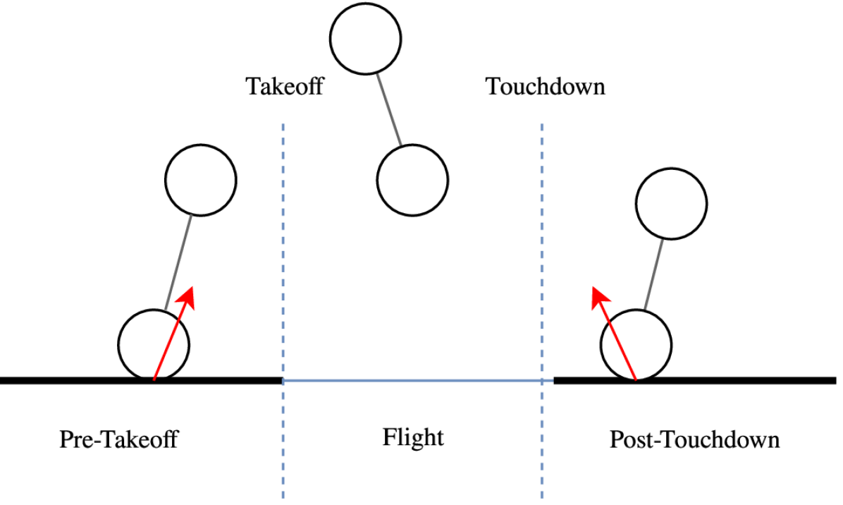
Next we setup task specific constraints. The start state and the target state are specified for knots and . At each knot point, state limits , and control limits are enforced. These limits ensure the physical feasibility of the motion generated. For different tasks the state and control limits will differ. For instance, when jumping over a gap, the state limits for the three phases will indicate where the “flight“ phase begins and ends. In general, a jumping motion involves three phases: a “pre-takeoff” phase, where the robot is on the ground, a “flight” phase where the robot is in the air, and a “post-touchdown” phase where the robot lands and re-balances. We specify the duration of each phases by setting the time of takeoff , and the time of touchdown .
Finally, we specify ground contact constraints. Contact forces must be zero () while the robot is in the flight phase. For the ground phases, they should stay inside the friction cone (, where is the friction coefficient) and have a positive vertical component (). For kinematics, we enforce a no-slip constraint while the robot is on the ground: , where is the wheel radius. For motions without jumping, we use a similar formulation by removing the flight phase related constraints.
The planner finds an admissible trajectory for the control task. However, for executing it on a real system or in simulation, a controller is needed.
III-B Control
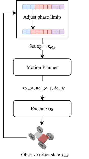
With open-loop control, the planned trajectory cannot be tracked precisely due to tracking error introduced by model mismatch and external perturbations. Thus, we use Model Predictive Control [18] to handle the errors. Figure 4 illustrates the scheme. At each timestep, the planner re-plans the trajectory starting at the observed robot state obtained from the simulator. Then, the first action of the plan is executed. After that, it recedes the time horizon by the elapsed time.
A natural problem arises with the recession of . Ideally we would keep the number of knot points constant—this enables saving the optimizer’s state and avoids costly re-initialization. The solution requires adjusting the limits of the problem so that each phase always has the same duration. Thus, we maintain the ratio of pre / flight / post phases by shifting the limits of the problem while keeping the same.
To implement the optimal control problem, we used CasADI [19]. As the underlying solver, we used KNITRO and selected the Interior/Conjugate-Gradient algorithm that is well-suited for large-scale sparse optimal control problems [20].
IV Simulation Results
In order to validate our approach, we investigated several tasks, namely swing-up, balancing and jumping in the physics simulator PyBullet [21]. Please find the accompanying video at https://youtu.be/j2sIWL8m2pQ.
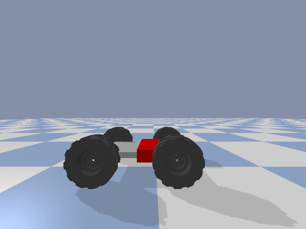
The simulated robot weighs including the wheels and the dimensions of the base are . The radius of the wheels is and wheels are wide.
IV-A Swing-up and Balance
Firstly, we demonstrate that the robot can switch from a driving mode on four wheels to a balancing mode on two wheels. This demonstrates that the robot can switch between modes without intervention. We used a two-stage controller for this task. Since controlling the robot in driving mode is outside the scope of this paper, we drive forward with a constant acceleration until we reach a velocity of . Then we switch to the proposed MPC scheme.
The trajectory duration (and MPC horizon) was with knot points. We set control limits to and for and , respectively. Figure 6 shows the resulting motion. The controller planned a motion where the robot coordinates its prismatic joint and wheel to swing-up.
IV-B Driving Upright
Next we demonstrate that, in the upright mode, the robot can balance and drive forward using the proposed approach. In this experiment, the goal is to drive the robot forward while balancing upright. We defined the same limits on the states , and the controls for the entire trajectory. We set torque limits for the wheels to and force limits for the prismatic joint to . The total time (MPC horizon) was and knot points.
The resulting motion is shown in Figure 8. We noticed that the optimizer first chooses to extend the prismatic joint before moving forward. This behavior can, for instance, be explained by noticing that it is easier to balance a body with a higher center of mass, which is achieved through extending the prismatic joint. Note that we did not in any way encode this behavior—the planner discovered it from first principles of optimization.
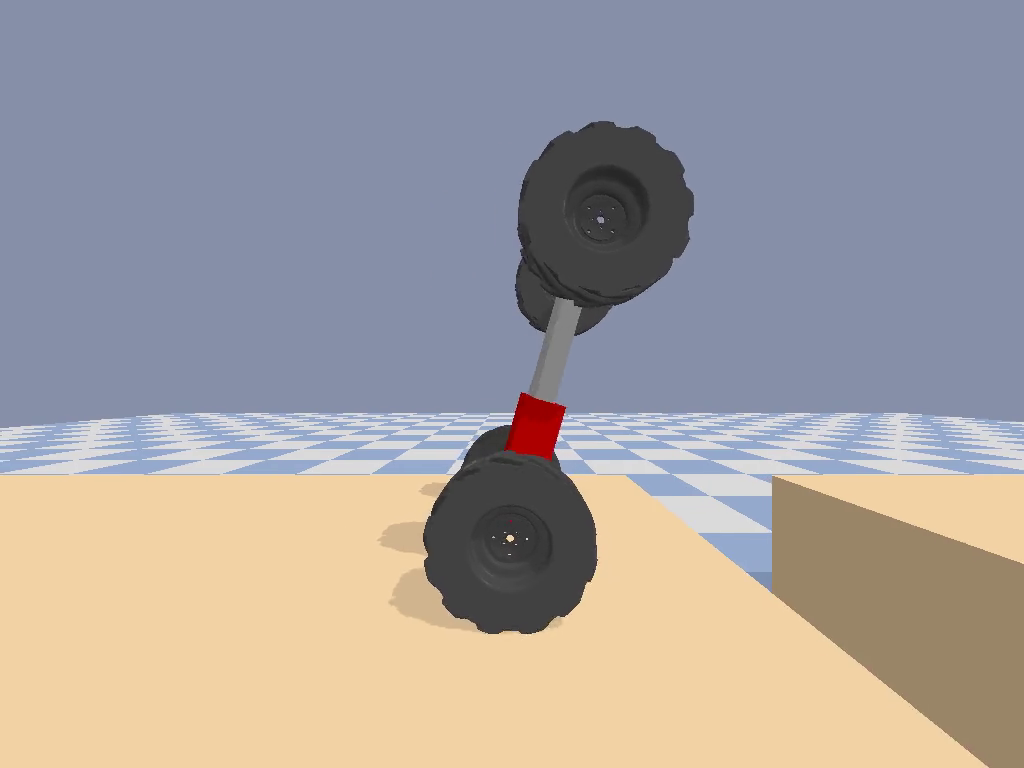
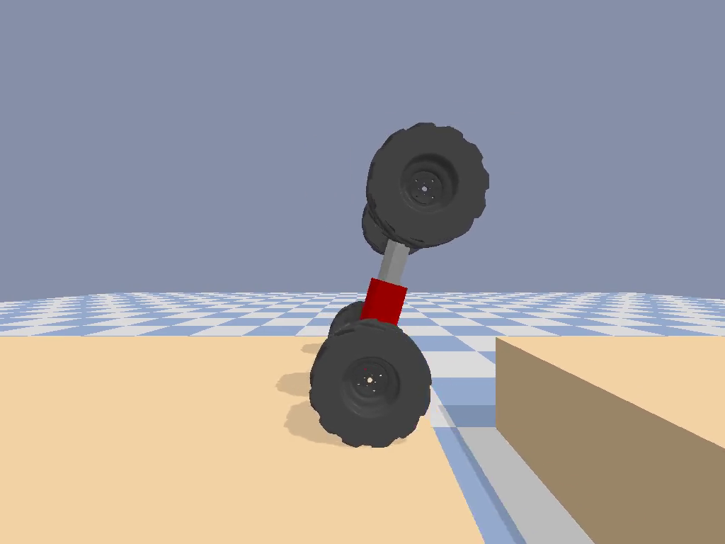
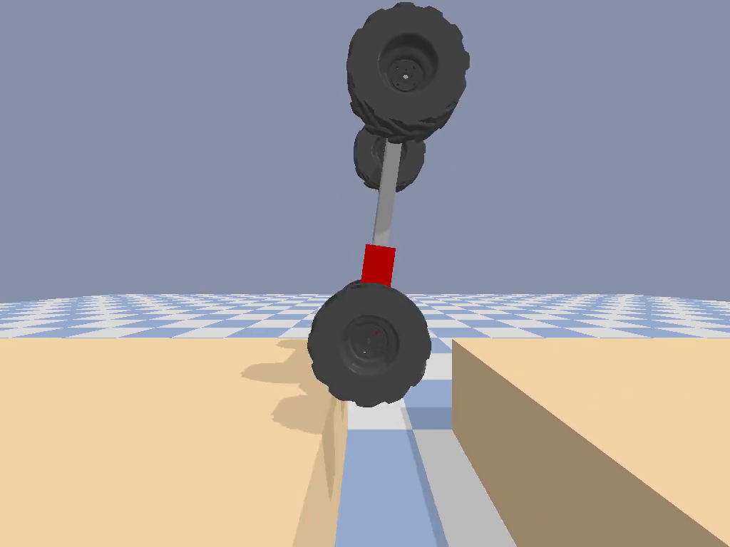
IV-C Jumping Over a Gap
Finally, we consider jumping over a gap, which uses the full multi-phase optimization described in section III. This task is more complex since different phases are involved in the motion.
We can entirely describe the jumping motion via state and control limits. In addition to torque limits and force limits , we set the state limits for each of the phases. Letting specify the bounds of the gap in the direction, we obtain:
| (7) | ||||
| (8) | ||||
| (9) |
where and are the limits of the prismatic joint, is the wheel radius, and limits the jumping height. In order to set up the length of the trajectory , we ran time optimization within bounds and knot points . This ensures that the optimizer chooses the appropriate flight duration that is physically feasible within the set time limits. In this sense, was the optimal time and MPC horizon.
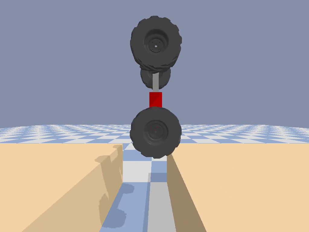
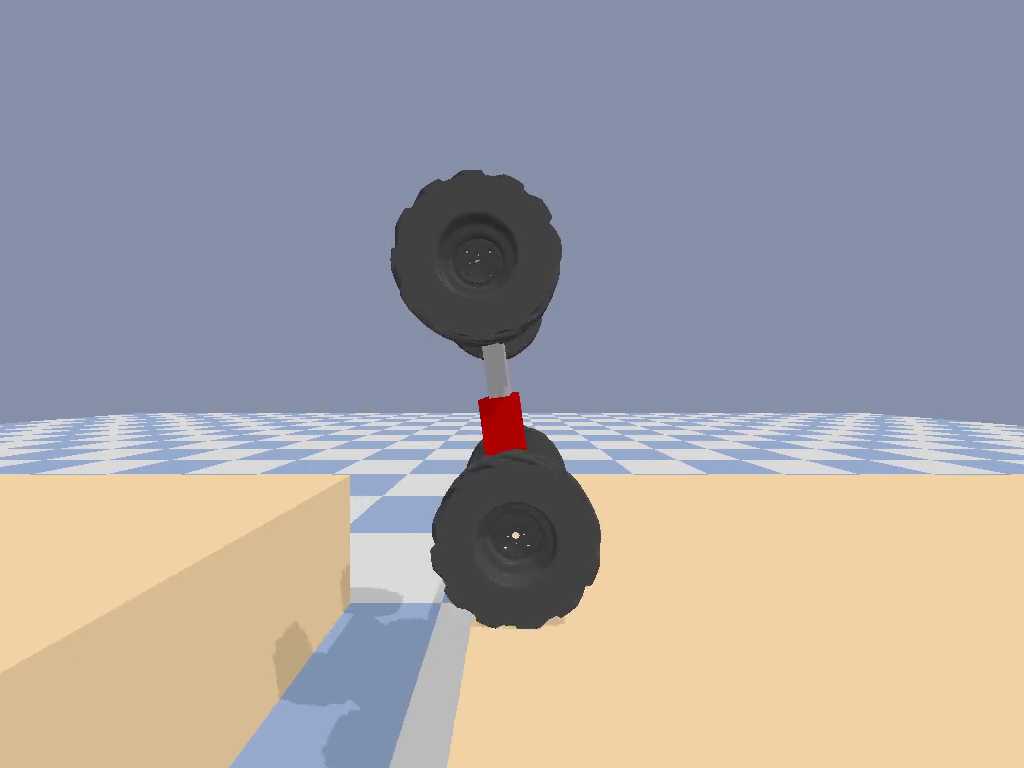
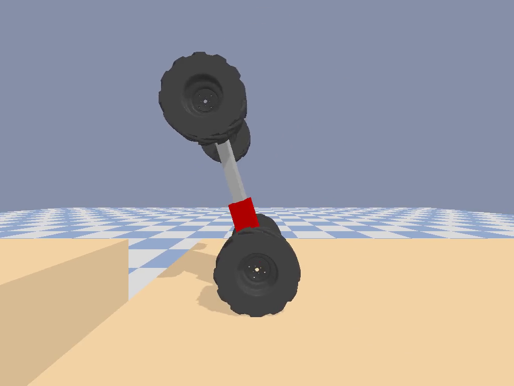
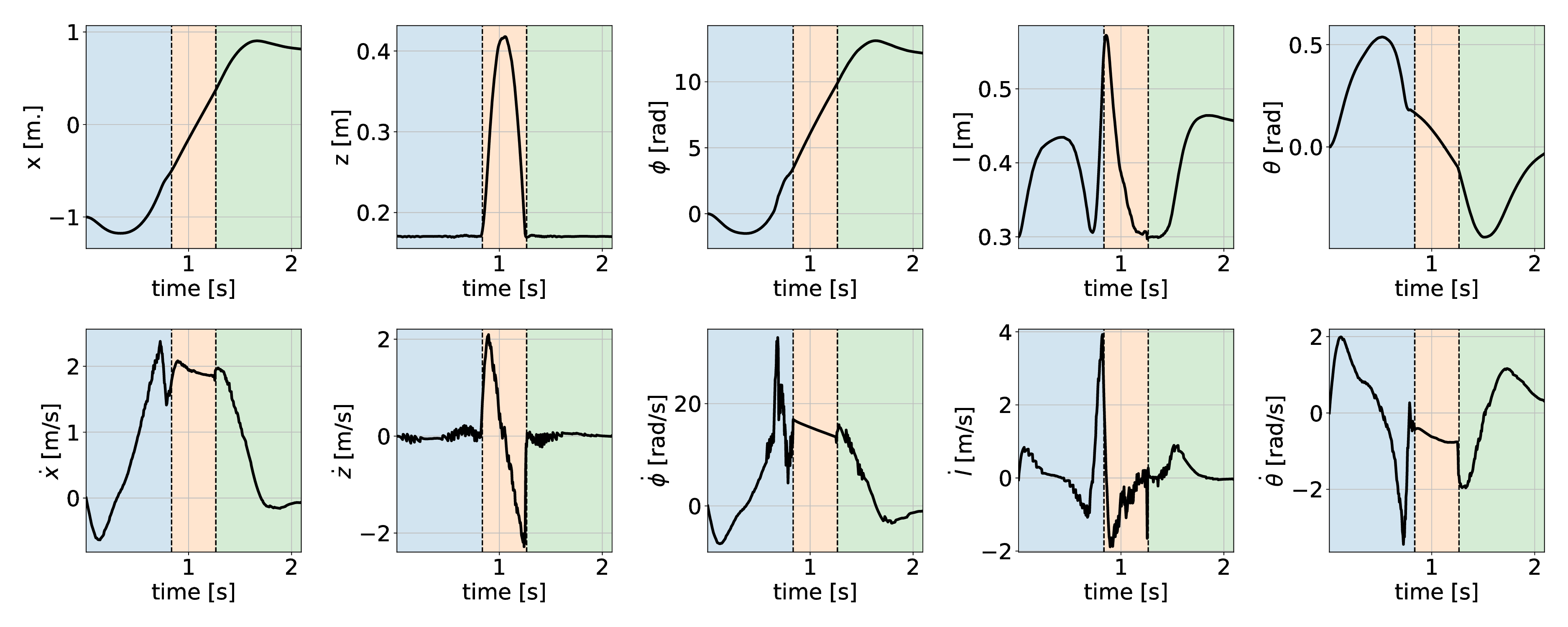
The resulting motion is shown in Figure 9 and its state and control history is plotted in Figure 10. The optimizer first “contracts” the body of the robot by retracting the prismatic joint before takeoff and extends it just before landing to absorb impact. We can see the preparatory movement in the optimized motion in Figure 9 for , and .
V Robustness
In the following experiments, we evaluate the robustness of the MPC approach as compared to a Proportional-Derivative (PD) controller with feed-forward torque.
The PD controller has the following control equation:
| (10) | ||||
| (11) |
where is the error between desired and measured state variables, , , , , , are the PD gains we tuned by hand. We add a term dependent on in the first equation so that position error is taken into account. Note, the larger PD gains for the prismatic joint—this is due to the scale difference in the length and force needed. We tuned the PD controller so that it achieves similar performance when driving on flat terrain as the MPC controller.
V-A Robustness to Sensor Noise
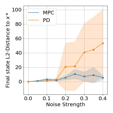
This experiment has the same setup as subsection IV-B. We compare the effects of sensor noise on both the MPC and the PD controllers. We added Gaussian noise to sensor readings at each timestep of the simulation:
| (12) |
where is the noise standard deviation, which was varied in the range and is the identity matrix. We computed the L2-distance from the observed state to the goal state at the end of the simulation. For this experiment we ran trials for each value of , computing the means as well as the standard deviations of the L2-distance. The results are in Figure 11.
We notice similar performance for the PD controller at lower noise strengths. However, at the PD controller has a significant drop in performance. Additionally, as the noise strength increases, the variability in performance for the PD controller becomes larger. In contrast, the MPC controller shows better mean performance and lower performance variability across values.
V-B Rough Terrain Locomotion
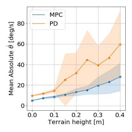
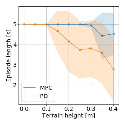
For this experiment we consider the task of driving forward on two wheels, as outlined in subsection IV-B. For the MPC controller we set a target velocity and horizon . The PD controller has no feed-forward torque reference; it has the same desired velocity target as well as a balance target . Neither have knowledge of the terrain and the overall duration of each experiment was .
We ran experiments for varied terrain heights in the range . We generated random terrain using Perlin noise for every experiment while keeping the same random number generator seed between the PD and MPC. Example generated terrain for heights and are shown in 13(a) and 13(b), respectively. We computed the mean absolute angle velocity for the entire trajectory for each of the terrain heights and its standard deviation. We also show the episode duration as well as one standard deviation. The episode is terminated when the angle of the robot is more than degrees. The results are in 12(a) and 12(b), respectively.
For flat terrain and for terrain height up to , MPC and PD show similar results. As the terrain height increases, however, MPC is better at stabilizing the robot with much less variability in performance.
VI Discussion and Future Work
The results demonstrated in this paper show that the VL-WIP model, regardless of its simplicity, is sufficient for generating complex dynamic motions. We consider the combined motion planning pipeline developed here as a first step towards more dynamic locomotion of hybrid wheel-legged systems. Future work will apply several connected VL-WIP models, one for each limb, to wheel-legged bipeds and quadrupeds, using the standard motion planning and control pipeline outlined here. This approach is similar to using a SLIP model for each limb of a biped [22, 23, 24]. Compared to single rigid-body models, like the one in [25], the stacked VL-WIP model will model leg mass and inertia properties, allowing for more complex in-air maneuvers as well as not requiring inertia compensation.
Furthermore, for all the motions the planner exploited the dynamics of the system without being guided to do so explicitly. Most notably for jumping it discovered the preparatory motion from optimization alone—including contracting and extending the robot before take off, absorbing the impact upon landing, and extending the prismatic joint for easier balancing.
Currently for swing up and jumping we have predefined the switching times. In the future these will be automatically discovered, for instance via phase-based parametrization [25, 26].
When transferring to a real system, we note that work needs to be done to increase the speed of the computation, for instance by warm-starting the solver using trajectory libraries [27] or using policy learning. Our MPC controller ran at Hz for balancing, Hz for jumping, and Hz for swing-up on a Intel Core i9-9980HK at with of DDR4 RAM at . We have indeed noticed that the solver did not take an equal number of iterations for all initial conditions and it sometimes did not converge. For this reason the speed was significantly lower on the more complex three-phase optimization for the jumping task. The convergence of the motion planner and the impact of warm starts is outside of the scope of this paper but it presents an exciting direction for future research.
Acknowledgements
This research is supported by the EPSRC Centre for Doctoral Training in Robotics and Autonomous Systems (EP/L016834/1), the EPSRC UK RAI Hub in Future AI and Robotics for Space (FAIR-SPACE, ID:EP/R026092/1) and the EU H2020 project Memory of Motion (MEMMO, ID: 780684). We would like to thank Henrique Ferollho and Matthew Timmons-Brown for their valuable help and feedback,
References
- [1] V. Klemm, A. Morra, C. Salzmann, F. Tschopp, K. Bodie, L. Gulich, N. Kung, D. Mannhart, C. Pfister, M. Vierneisel, F. Weber, R. Deuber, and R. Siegwart, “Ascento: A Two-Wheeled Jumping Robot,” in 2019 International Conference on Robotics and Automation (ICRA). Montreal, QC, Canada: IEEE, May 2019, pp. 7515–7521.
- [2] M. Bjelonic, P. K. Sankar, C. D. Bellicoso, H. Vallery, and M. Hutter, “Rolling in the Deep – Hybrid Locomotion for Wheeled-Legged Robots using Online Trajectory Optimization,” arXiv:1909.07193 [cs, eess], Jan. 2020.
- [3] M. Bjelonic, C. D. Bellicoso, Y. de Viragh, D. Sako, F. D. Tresoldi, F. Jenelten, and M. Hutter, “Keep Rollin’ - Whole-Body Motion Control and Planning for Wheeled Quadrupedal Robots,” IEEE Robotics and Automation Letters, vol. 4, no. 2, pp. 2116–2123, Apr. 2019.
- [4] M. Geilinger, R. Poranne, R. Desai, B. Thomaszewski, and S. Coros, “Skaterbots: optimization-based design and motion synthesis for robotic creatures with legs and wheels,” ACM Transactions on Graphics, vol. 37, no. 4, pp. 1–12, July 2018.
- [5] M. Giftthaler, F. Farshidian, T. Sandy, L. Stadelmann, and J. Buchli, “Efficient kinematic planning for mobile manipulators with non-holonomic constraints using optimal control,” in 2017 IEEE International Conference on Robotics and Automation (ICRA), May 2017, pp. 3411–3417.
- [6] P. R. Giordano, M. Fuchs, A. Albu-Schaffer, and G. Hirzinger, “On the kinematic modeling and control of a mobile platform equipped with steering wheels and movable legs,” in 2009 IEEE International Conference on Robotics and Automation, May 2009, pp. 4080–4087.
- [7] K. Nagano and Y. Fujimoto, “The stable wheeled locomotion in low speed region for a wheel-legged mobile robot,” in 2015 IEEE International Conference on Mechatronics (ICM), Mar. 2015, pp. 404–409.
- [8] R. Tedrake, “Underactuated Robotics,” Feb. 2018. [Online]. Available: http://underactuated.mit.edu/
- [9] D. E. Orin, A. Goswami, and S.-H. Lee, “Centroidal dynamics of a humanoid robot,” Autonomous Robots, vol. 35, no. 2, pp. 161–176, Oct. 2013.
- [10] Y. de Viragh, M. Bjelonic, C. D. Bellicoso, F. Jenelten, and M. Hutter, “Trajectory Optimization for Wheeled-Legged Quadrupedal Robots Using Linearized ZMP Constraints,” IEEE Robotics and Automation Letters, vol. 4, no. 2, pp. 1633–1640, Apr. 2019, conference Name: IEEE Robotics and Automation Letters.
- [11] A. Saunders, C. E. Thorne, and A. A. Rizzi, “Environmentally sealed combustion powered linear actuator,” US Patent US9 238 967B2, 2012.
- [12] T. Tanaka and S. Hirose, “Development of leg-wheel hybrid quadruped “AirHopper” design of powerful light-weight leg with wheel,” in 2008 IEEE/RSJ International Conference on Intelligent Robots and Systems, Sept. 2008, pp. 3890–3895.
- [13] I. Poulakakis and J. W. Grizzle, “The Spring Loaded Inverted Pendulum as the Hybrid Zero Dynamics of an Asymmetric Hopper,” IEEE Transactions on Automatic Control, vol. 54, no. 8, pp. 1779–1793, Aug. 2009.
- [14] P. M. Wensing and D. E. Orin, “Development of high-span running long jumps for humanoids,” in 2014 IEEE International Conference on Robotics and Automation (ICRA), May 2014, pp. 222–227.
- [15] R. P. M. Chan, K. A. Stol, and C. R. Halkyard, “Review of modelling and control of two-wheeled robots,” Annual Reviews in Control, vol. 37, no. 1, pp. 89–103, Apr. 2013.
- [16] Y. Ding, J. Gafford, and M. Kunio, “Modeling, Simulation and Fabrication of a Balancing Robot,” p. 22, 2012.
- [17] M. Kelly, “An Introduction to Trajectory Optimization: How to Do Your Own Direct Collocation,” SIAM Review, vol. 59, no. 4, pp. 849–904, Jan. 2017.
- [18] J. B. Rawlings, D. Q. Mayne, and M. Diehl, Model predictive control: theory, computation, and design. Nob Hill Publishing Madison, WI, 2017, vol. 2.
- [19] J. Andersson, J. Åkesson, and M. Diehl, “CasADi: A Symbolic Package for Automatic Differentiation andOptimal Control,” in Recent Advances in Algorithmic Differentiation, ser. Lecture Notes in Computational Science and Engineering, S. Forth, P. Hovland, E. Phipps, J. Utke, and A. Walther, Eds. Berlin, Heidelberg: Springer, 2012, pp. 297–307.
- [20] R. H. Byrd, J. Nocedal, and R. A. Waltz, “Knitro: An Integrated Package for Nonlinear Optimization,” in Large-Scale Nonlinear Optimization, P. Pardalos, G. Di Pillo, and M. Roma, Eds. Boston, MA: Springer US, 2006, vol. 83, pp. 35–59.
- [21] E. Coumans and Y. Bai, “Pybullet, a python module for physics simulation for games, robotics and machine learning,” GitHub repository, 2016.
- [22] P. M. Wensing and D. E. Orin, “High-speed humanoid running through control with a 3D-SLIP model,” in 2013 IEEE/RSJ International Conference on Intelligent Robots and Systems, Nov. 2013, pp. 5134–5140.
- [23] ——, “3D-SLIP steering for high-speed humanoid turns,” in 2014 IEEE/RSJ International Conference on Intelligent Robots and Systems, Sept. 2014, pp. 4008–4013.
- [24] Y. Liu, P. M. Wensing, D. E. Orin, and Y. F. Zheng, “Dynamic walking in a humanoid robot based on a 3D Actuated Dual-SLIP model,” in 2015 IEEE International Conference on Robotics and Automation (ICRA), May 2015, pp. 5710–5717.
- [25] A. W. Winkler, C. D. Bellicoso, M. Hutter, and J. Buchli, “Gait and Trajectory Optimization for Legged Systems Through Phase-Based End-Effector Parameterization,” IEEE Robotics and Automation Letters, vol. 3, no. 3, pp. 1560–1567, July 2018.
- [26] T. Stouraitis, I. Chatzinikolaidis, M. Gienger, and S. Vijayakumar, “Dyadic collaborative manipulation through hybrid trajectory optimization.” in CoRL, 2018, pp. 869–878.
- [27] W. Merkt, V. Ivan, and S. Vijayakumar, “Leveraging Precomputation with Problem Encoding for Warm-Starting Trajectory Optimization in Complex Environments,” in IEEE/RSJ IROS, Oct 2018, pp. 5877–5884.
- [28] D. Morin, Introduction to classical mechanics: with problems and solutions. Cambridge University Press, 2008.
We use the Lagrangian method to derive the dynamics of the system [28, Chapter 6]. First, we define the position of the mass and its velocity :
| (13) | ||||
Lagrange’s method states that for a system with total kinetic energy and potential energy :
| (14) |
where is the system’s Lagrangian and are external forces applied to the system. We now need to compute the system’s kinetic and potential energy.
In general, every link will have a rotational and translational kinetic energy component. For the wheel we include a rotational kinetic energy term where is the moment of inertia of the wheel. Since the point mass has a zero moment of inertia, it only has a translational kinetic energy , where is the velocity of the point mass.