Abstract

Consensus-based distributed optimization methods have recently been advocated as alternatives to parameter server and ring all-reduce paradigms for large scale training of machine learning models. In this case, each worker maintains a local estimate of the optimal parameter vector and iteratively updates it by averaging the estimates obtained from its neighbors, and applying a correction on the basis of its local dataset. While theoretical results suggest that worker communication topology should have strong impact on the number of epochs needed to converge, previous experiments have shown the opposite conclusion. This paper sheds lights on this apparent contradiction and show how sparse topologies can lead to faster convergence even in the absence of communication delays.

1 INTRODUCTION

In 2014, Google’s Sybil machine learning (ML) platform was processing hundreds of terabytes through thousands of cores to train models with hundreds of billions of parameters (Canini et al., 2014). At this scale, no single machine can solve these problems in a timely manner, and, as time goes on, the need for efficient distributed solutions becomes even more urgent. For example, experiments in (Young et al., 2017) rely on more than $10^{4}$ computing nodes to iteratively improve the (hyper)parameters of a deep neural network.

The example in (Young et al., 2017) is typical of a large class of iterative ML distributed algorithms. Such algorithms begin with a guess of an optimal vector of parameters and proceed through multiple iterations over the input data to improve the solution. The process evolves in a data-parallel manner: input data is divided among worker threads. Currently, two communication paradigms are commonly used to coordinate the different workers (Google I/O, 2018): parameter server and ring all-reduce. Both paradigms are natively supported by TensorFlow (Abadi et al., 2016).

In the first case, a stateful parameter server (PS) (Smola and Narayanamurthy, 2010) maintains the current version of the model parameters. Workers use locally available versions of the model to compute “delta” updates of the parameters (e.g., through a gradient descent step). Updates are then aggregated by the parameter server and combined with its current state to produce a new estimate of the optimal parameter vector.

As an alternative, it is possible to remove the PS, by letting each worker aggregate the inputs of all other workers through the ring all-reduce algorithm (Gibiansky, 2017). With $M$ workers, each aggregation phase requires $2(M-1)$ communication steps with $\mathcal{O}(1)$ data transmitted per worker. There are many efficient low level implementations of ring all-reduce, e.g., in NVIDIA’s library NCCL.

We observe that both the PS and the ring all-reduce paradigms 1) maintain a unique candidate parameter vector at any given time and 2) rely logically on an all-to-all communication scheme. Recently Lian et al. (2017, 2018) have promoted an alternative approach in the ML research community, where each worker 1) keeps updating a local version of the parameters and 2) broadcasts its updates only to a subset of nodes (its neighbors). This family of algorithms became originally popular in the control community, starting from the seminal work of Tsitsiklis et al. (1986) on distributed gradient methods. They are often referred to as consensus-based distributed optimization methods. Experimental results in (Lian et al., 2017, 2018; Luo et al., 2019) show that

1. in terms of number of epochs, the convergence speed is almost the same when the communication topology is a ring or a clique, contradicting theoretical findings that predict convergence to be faster on a clique;

2. in terms of wall-clock time, convergence is faster for sparser topologies, an effect attributed in (Lian et al., 2017) to smaller communication load.

In particular, Luo et al. (2019) summarize their findings as follows “in theory, the bigger the spectral gap, [i.e., the more connected the topology] the fewer iterations it takes to converge. However, our experiments do not show a significant difference in the convergence rate w.r.t. iterations, even when spectral gaps are very dissimilar.”

In this paper we contribute to a better understanding of the potential advantages of consensus-based gradient methods. In particular,

1. we present a refined convergence analysis that helps to explain the apparent contradiction among theoretical results and empirical observations,

2. we show that sparse topologies can speed-up wall-clock time convergence even when communication costs are negligible, because they intrinsically mitigate the straggler problem.

The paper is organized as follows. Section 2 provides required background. Our theoretical analysis of the effect of communication topology is in Sect. 3. Experiment results in Sect. 4 confirm our findings. Section 5 concludes the paper.

2 NOTATION AND BACKGROUND

The goal of supervised learning is to learn a function that maps an input to an output using $S$ examples from a training dataset ${\mathbb{S}}=\{({\bm{x}}^{(l)},y^{(l)}),l=1,\dots S\}$. Each example $({\bm{x}}^{(l)},y^{(l)})$ is a pair consisting of an input object ${\bm{x}}^{(l)}$ and an associated target value $y^{(l)}$. In order to find the best statistical model, ML techniques often find the set of parameters ${\bm{w}}\in\mathbb{R}^{n}$ that solves the following optimization problem:

$$\operatorname*{minimize}_{\bm{w}}\;\;\sum_{l=1}^{S}f({\bm{w}},{\bm{x}}^{(l)},y^{(l)})$$ (1)

where function $f({\bm{w}},{\bm{x}}^{(l)},y^{(l)})$ represents the error the model commits on the $l$-th element of the dataset ${\mathbb{S}}$ when parameter vector ${\bm{w}}$ is used. The objective function may also include a regularization term that enforces some “simplicity” (e.g., sparseness) on ${\bm{w}}$; such a term is easily taken into account in our analysis.

Due to increases in available data and statistical model complexity, distributed solutions are often required to determine the parameter vector in a reasonable time. The dataset in this case is divided among $M$ workers (${\mathbb{S}}=\cup_{j=1}^{M}{\mathbb{S}}_{j}$), possibly with some overlap. For simplicity, we consider that all local datasets ${\mathbb{S}}_{j}$ have the same size. Problem (1) can be restated in an equivalent form as minimization of the sum of functions local to each node:

$$\operatorname*{minimize}_{\bm{w}}\;\;F({\bm{w}})=\sum_{j=1}^{M}F_{j}({\bm{w}}),$$ (2)

where $F_{j}({\bm{w}})=\frac{1}{|{\mathbb{S}}_{j}|}\sum_{({\bm{x}}^{(l)},y^{(l)})\in{\mathbb{S}}_{j}}f({\bm{w}},{\bm{x}}^{(l)},y^{(l)})$.

The distributed system can be represented by a directed dataflow graph ${\mathcal{G}}=(\mathcal{V},\mathcal{E})$, where $\mathcal{V}=\{1,2,\dots M\}$ is the set of nodes (the workers) and an edge $(i,j)\in\mathcal{E}$ indicates that, at each iteration, node $j$ waits for updates from node $i$ for the previous iteration. We assume the graph is strongly connected. Let $N_{j}=\{i|(i,j)\in\mathcal{E}\}$ denote the in-neighborhood of node $j$, i.e., the set of predecessors of node $j$ in ${\mathcal{G}}$. Each node $j$ maintains a local estimate of the parameter vector ${\bm{w}}_{j}(k)$ and broadcasts it to its successors. The local estimate is updated as follows:

$${\bm{w}}_{j}(k+1)=\sum_{i\in N_{j}\cup\{j\}}{\bm{w}}_{i}(k){A}_{i,j}-\eta(k){\bm{g}}_{j}({\bm{w}}_{j}(k)).$$ (3)

The node computes a weighted average (consensus/gossip component) of the estimates of its neighbors and itself, and then corrects it taking into account a stochastic subgradient ${\bm{g}}_{j}({\bm{w}}_{j}(k))$ of its local function, i.e.,

$${\bm{g}}_{j}({\bm{w}}_{j}(k))=\frac{1}{B}\sum_{({\bm{x}}^{(l)},y^{(l)})\in\xi_{j}(k)}\partial f({\bm{w}}_{j}(k),{\bm{x}}^{(l)},y^{(l)}),$$

where $\partial f({\bm{w}},{\bm{x}}^{(l)},y^{(l)})$ denotes a subgradient of $f$ with respect to ${\bm{w}}$, and $\xi_{j}(k)$ is a random minibatch of size $B$ drawn from ${\mathbb{S}}_{j}$. Parameter $\eta(k)>0$ is the (potentially time-varying) learning rate. ${\bm{A}}=({A}_{i,j})$ is an $M\times M$ matrix of non-negative weights. We call ${\bm{A}}$ the consensus matrix.

The operation of a synchronous PS or ring all-reduce is captured by (3) when the underlying graph $\mathcal{G}$ is a clique, ${\bm{A}}={\bf 1}{\bf 1}^{\intercal}/M$, where $\bf 1$ is the $M\times 1$ vector consisting of all ones, and ${\bm{w}}_{i}(0)={\bm{w}}_{j}(0),\forall i,j\in\mathcal{V}$.

Under some standard technical conditions, (Nedić et al., 2018, Thm. 8) and (Duchi et al., 2012, Thm. 2) conclude, respectively for Distributed Subgradient Method (DSM) and for the Dual Averaging Distributed method, that the number of iterations $K_{\epsilon}$ needed to approximate the minimum objective function value by the desired error $\epsilon$ is

$$K_{\epsilon}\in\mathcal{O}\!\left(\frac{1}{\epsilon^{2}\gamma({\bm{A}})}\right),$$ (4)

where $0\leq\gamma({\bm{A}})\leq 1$ is the spectral gap of the matrix ${\bm{A}}$, i.e., the difference between the moduli of the two largest eigenvalues of ${\bm{A}}$. The spectral gap quantifies how information flows in the network. In particular, the spectral gap is maximal for a clique with weights $A_{i,j}=1/M$. Motivated by these convergence results, existing theoretically-oriented literature has concluded that a more connected network topology leads to faster convergence (Nedić et al., 2018; Duchi et al., 2012). But some recent experimental results report that consensus-based gradient methods achieve similar performance after the same number of iterations/epochs on topologies as different as rings and cliques. For example (Lian et al., 2017, Fig. 3) shows almost overlapping training losses for different ResNet architectures trained on CIFAR-10 with up to one hundred workers. (Luo et al., 2019, Fig. 20), (Koloskova et al., 2019, Fig. 11 in supplementary material), and our experimental results in Sect. 4 confirm these findings.

Lian et al. (2017) provide a partial explanation for this insensitivity in their Corollary 2, showing that the convergence rate is topology-independent 1) after a large number of iterations ($\mathcal{O}(M^{5}/\gamma({\bm{A}})^{2})$), 2) for a vanishing learning rate, and 3) when the functions $F_{j}$ are differentiable with Lipschitzian gradients. Under the additional hypothesis of strong convexity, Pu et al. (2019) prove that topology insensitivity should manifest after $\mathcal{O}(M/\gamma({\bm{A}})^{2})$ iterations. Assran et al. (2019) provide similar results in terms of the graph diameter and maximum degree. These results do not explain why insensitivity is often observed in practice (as shown in (Lian et al., 2017, 2018; Luo et al., 2019; Koloskova et al., 2019)) 1) since the beginning of the training phase, 2) with constant learning rates, and 3) for non-differentiable machine learning models (e.g., neural networks). In the following section, we present a refined convergence analysis that explains when and why the effect of topology on the number of iterations needed to converge is weaker than what previously predicted.

3 ANALYSIS

A less connected topology requires more iterations to achieve a given precision as indicated by (4). Our detailed analysis below shows that, when consensus-based optimization methods are used for ML training, the increase in the number of iterations is much less pronounced than previous studies predict. This is due to two different effects. First, consensus is affected only by variability in initial estimates and subgradients across nodes, and not by their absolute values. Second, certain configurations of initial estimates and subgradients are more difficult to achieve a consensus over, and would make the training highly dependent on the topology, but they are unlikely to be obtained by randomly partitioning the dataset.

Let $n$ be the number of parameters of the model, and ${\bm{W}}(k)$ and ${\bm{G}}(k)$ be $n\times M$ matrices, whose columns are, respectively, node estimates ${\bm{w}}_{1}(k),\dots,{\bm{w}}_{M}(k)$ and subgradients ${\bm{g}}_{1}({\bm{w}}_{1}(k)),\dots,{\bm{g}}_{M}({\bm{w}}_{M}(k))$ at the completion of iteration $k$. Equation (3) can be rewritten in the form ${\bm{W}}(k+1)={\bm{W}}(k){\bm{A}}-\eta(k){\bm{G}}(k)$, from which we obtain iteratively

$${\bm{W}}(k+1)={\bm{W}}(0){\bm{A}}^{k+1}-\sum_{h=0}^{k}\eta(h){\bm{G}}(h){\bm{A}}^{k-h}.$$ (5)

We make the following assumptions:

A1

all functions $F_{i}$ are convex,

A2

the set of (global) minimizers ${\mathbb{W}}^{*}$ is non-empty,

A3

graph ${\mathcal{G}}$ is strongly connected,

A4

matrix ${\bm{A}}$ is normal (i.e., ${\bm{A}}^{\intercal}{\bm{A}}={\bm{A}}{\bm{A}}^{\intercal}$) and doubly stochastic,

A5

the squared Frobenius norm of subgradient matrix ${\bm{G}}(k)$ is bounded in expectation over the vector $\bm{\xi}$ of minibatches randomly drawn at nodes, i.e., there exists $E$, such that $\operatorname{\mathbb{E}}_{\bm{\xi}}\left[\left\lVert{\bm{G}}(k)\right\rVert_{F}^{2}\right]\leq E$.

Assumptions A1-A4 are standard ones in the related literature, see for example (Nedić and Ozdaglar, 2009; Duchi et al., 2012; Nedić et al., 2018). Assumption A5 imposes a bound on the (expected) energy of the subgradients, because $\left\lVert{\bm{G}}(k)\right\rVert_{F}^{2}=\sum_{j}\left\lVert{\bm{g}}_{j}({\bm{w}}_{j}(k))\right\rVert_{2}^{2}$. In the literature it is often replaced by the stronger requirement that the norm-2 of the subgradients ${\bm{g}}_{j}({\bm{w}}_{j}(k))$ is bounded. Let $\Delta{\bm{G}}(k)$ denote the matrix ${\bm{G}}(k)-{\bm{G}}(k){\bm{1}}{\bm{1}}^{\intercal}/{M}$, whose column $j$ is the difference between subgradient ${\bm{g}}_{j}({\bm{w}}_{j}(k))$ and the average of subgradients $\sum_{j=1}^{M}{\bm{g}}_{j}({\bm{w}}_{j}(k))/M$. $\left\lVert\Delta{\bm{G}}(k)\right\rVert_{F}^{2}$ captures the variability in the subgradients. Assumption A5 also implies that there exist two constants $E_{\textrm{sp}}\leq E$ and $H\leq\sqrt{E}$ such that

$$\operatorname{\mathbb{E}}_{\bm{\xi}}\left[\left\lVert\Delta{\bm{G}}(k)\right\rVert_{F}^{2}\right]\leq E_{\textrm{sp}},\;\;\;\left\lVert\operatorname{\mathbb{E}}_{\bm{\xi}}\left[{\bm{G}}(k)\right]\right\rVert_{F}\leq H.$$

Similarly, let $R$ denote the energy of the initial parameter vectors (or an upper bound for it), i.e., $R\triangleq\left\lVert{\bm{W}}(0)\right\rVert_{F}^{2}$. We also denote by $R_{\textrm{sp}}$ the energy for the difference matrix $\Delta{\bm{W}}(0)\triangleq{\bm{W}}(0)-{\bm{W}}(0){\bm{1}}{\bm{1}}^{\intercal}/M$, i.e.,  $R_{\textrm{sp}}\triangleq\left\lVert\Delta{\bm{W}}(0)\right\rVert_{F}^{2}$. $R_{\textrm{sp}}$ captures the variability in initial estimates. It holds $R_{\textrm{sp}}\leq R$.

Because of Assumption A4, the consensus matrix has a spectral decomposition with orthogonal projectors ${\bm{A}}=\sum_{q=1}^{Q}\lambda_{q}{\bm{P}}_{q},$ where $\lambda_{1},\dots,\lambda_{Q}$ are the $Q\leq M$ distinct eigenvalues of ${\bm{A}}$, ${\bm{P}}_{q}$ is the orthogonal projector onto the nullspace of ${\bm{A}}-\lambda_{q}{\bm{I}}$ along the range of ${\bm{A}}-\lambda_{q}{\bm{I}}$. We assume that the eigenvalues are ordered so that $|\lambda_{1}|\geq|\lambda_{2}|\geq\dots\geq|\lambda_{Q}|$. Assumptions A3 and A4 imply that $\lambda_{1}=1$, and $|\lambda_{2}|<1$ (Appendix B). Finally, we define

$$\alpha\triangleq\begin{cases}\sqrt{\sum_{q=2}^{Q}e_{q}\left|\frac{\lambda_{q}}{\lambda_{2}}\right|^{2}},&\textrm{if }\lambda_{2}\neq 0,\\ 1,&\textrm{otherwise.}\end{cases}$$ (6)

where $e_{q}$ is an upper-bound for the normalized fraction of energy $\operatorname{\mathbb{E}}_{\bm{\xi}}\left[\left\lVert\Delta{\bm{G}}(k)\right\rVert_{F}^{2}\right]$ in the subspace defined by projector ${\bm{P}}_{q}$ (Appendix D). The quantity $\alpha$ can be interpreted as an effective bound for the fraction of the energy $E_{\textrm{sp}}$ that falls in the subspace relative to the second largest eigenvalue $\lambda_{2}$.

We are now ready to introduce our main convergence result. We state it for the average model over nodes and time, i.e., for $\hat{\overline{\bm{w}}}(K-1)\triangleq\frac{1}{K}\sum_{k=0}^{K-1}\frac{1}{M}\sum_{i=1}^{M}{\bm{w}}_{i}(k)$. We have also derived a similar bound for the local time-average model at each node, i.e., for $\hat{\bm{w}}_{i}(K-1)\triangleq\frac{1}{K}\sum_{k=0}^{K-1}{\bm{w}}_{i}(k)$ (Appendix D.3).

Proposition 3.1.

Under assumptions A1-A5 and that a constant learning rate $\eta(k)=\eta$ is used, an upper bound for the objective value at the end of the ($K-1$)th iteration is given by:

$$\operatorname{\mathbb{E}}\left[F\!\left(\hat{\overline{\bm{w}}}(K-1)\right)\right]-F^{*}\leq\frac{M}{2\eta{K}}{\operatorname{\mathrm{dist}}{\!\left(\hat{\overline{\bm{w}}}(0),{\mathbb{W}}^{*}\right)}}^{2}+\frac{\eta E}{2}$$

$$\phantom{123}+2H\sqrt{R_{\textrm{sp}}}\frac{\sqrt{M}}{K}\frac{1-|\lambda_{2}|^{K}}{1-|\lambda_{2}|}$$

$$\phantom{123}+2\eta H\sqrt{E_{\textrm{sp}}}\left((1-\alpha)\frac{K-1}{K}\right.$$ (7)

$$\phantom{123+2\eta H\sqrt{E_{\textrm{sp}}}\left(\right.}\left.+\frac{\alpha}{1-|\lambda_{2}|}\left(1-\frac{1}{K}\frac{1-|\lambda_{2}|^{K}}{1-|\lambda_{2}|}\right)\right).$$

Here, $\operatorname{\mathrm{dist}}{\!\left({\bm{x}},{\mathbb{W}}^{*}\right)}$ denotes the Euclidean distance between vector ${\bm{x}}$ and set of global minimizers ${\mathbb{W}}^{*}$. The proof is in Appendix D.1. The first two terms on the right hand side of (7) also appear when studying the convergence of centralized subgradient methods. The last two terms appear because of the distributed consensus component of the algorithm and depend on $|\lambda_{2}|<1$. We observe that $1-|\lambda_{2}|$ is the spectral gap of ${\bm{A}}$. It measures how well connected the graph is. In particular, the larger the spectral gap (the smaller $\lambda_{2}$), the better the connectivity and the smaller the bound in (7).

From Proposition 3.1, we can derive a looser bound analogous to the bound for DSM in (Nedić and Ozdaglar, 2009). In fact, observing that $R_{\textrm{sp}}\leq R$, $E_{\textrm{sp}}\leq E$, $H\leq\sqrt{E}$, and $0\leq\alpha\leq 1$, we can prove (Appendix D.2):

Corollary 3.2.

Under assumptions A1-A5 and that constant learning rate $\eta(k)=\eta$ is used, an upper bound for the objective value at the end of the ($K-1$)th iteration is given by:

$$\operatorname{\mathbb{E}}\left[F\!\left(\hat{\overline{\bm{w}}}(K-1)\right)\right]-F^{*}\leq\frac{M}{2\eta{K}}{\operatorname{\mathrm{dist}}{\!\left(\hat{\overline{\bm{w}}}(0),{\mathbb{W}}^{*}\right)}}^{2}+\frac{\eta E}{2}$$

$$\phantom{12345}+2\sqrt{E}\sqrt{R}\frac{\sqrt{M}}{K}\frac{1-|\lambda_{2}|^{K}}{1-|\lambda_{2}|}$$

$$\phantom{12345}+2\eta E\frac{1}{1-|\lambda_{2}|}\left(1-\frac{1}{K}\frac{1-|\lambda_{2}|^{K}}{1-|\lambda_{2}|}\right).$$ (8)

In particular, if workers compute full-batch subgradients and the 2-norm of subgradients of functions $F_{i}$ is bounded by a constant $L$, we obtain:

$$F\!\left(\hat{\overline{\bm{w}}}(K-1)\right)-F^{*}\leq\frac{M}{2\eta{K}}{\operatorname{\mathrm{dist}}{\!\left(\hat{\overline{\bm{w}}}(0),{\mathbb{W}}^{*}\right)}}^{2}+\frac{\eta ML^{2}}{2}$$

$$\phantom{12345}+2L\sqrt{R}\frac{M}{K}\frac{1-|\lambda_{2}|^{K}}{1-|\lambda_{2}|}$$

$$\phantom{12345}+2\eta L^{2}\frac{M}{1-|\lambda_{2}|}\left(1-\frac{1}{K}\frac{1-|\lambda_{2}|^{K}}{1-|\lambda_{2}|}\right).$$ (9)

When $K$ is large enough, the fourth term in (8) and (9) is dominant, so that the error is essentially proportional to $1/(1-|\lambda_{2}|)$. Note that the constant multiplying $1/(1-|\lambda_{2}|)$ in (8) is larger than the corresponding one in (7) by a factor

$$\beta\triangleq\frac{1}{\alpha}\times\frac{E}{\sqrt{E_{\textrm{sp}}}H}$$ (10)

The value $\beta$ roughly indicates how much looser bound (8) is in comparison to bound (7).

Existing theoretical works like (Nedić and Ozdaglar, 2009; Duchi et al., 2012; Nedić et al., 2018) derived bounds similar to (9) and concluded then that one should select the learning rate proportional to $\sqrt{1-|\lambda_{2}|}$ to reduce the effect of topology. In particular, one obtains (4) when $\eta=\eta_{0}\sqrt{(1-|\lambda_{2}|)/K}$. Our bound (7) improves bound (8) by replacing $R$ in the third terms of (8) by the smaller value $R_{\textrm{sp}}$, and $\sqrt{E}$ in the third and fourth terms by the smaller values $H$ and $\sqrt{E_{\textrm{sp}}}$, and introducing the new coefficient $\alpha$. We qualitatively describe the effect of these constants.

$\mathbf{R_{\textrm{sp}}}$

Bound (7) shows that the norm of the initial estimates ($R$) does not really matter, but rather variability among workers does. In particular, for ML computation we can make ${\bm{w}}_{i}(0)={\bm{w}}_{j}(0)$ for each $i$ and $j$, and then $R_{\textrm{sp}}=0$, so that the third term in the RHS of (7) vanishes.

$\mathbf{E_{\textrm{sp}},H}$

For $E_{\textrm{sp}}$, considerations similar to those applying to $R_{\textrm{sp}}$ hold. What matters is the variability of the subgradients. Assume that the dataset is replicated at each node and each node computes the subgradient over the full batch ($B=S$). In this case all subgradients would be equal, and $\left\lVert\Delta{\bm{G}}(k)\right\rVert=0$, $E_{\textrm{sp}}=0$, and the fourth term would also vanish. This corresponds to the fact that, when initial parameter vectors, as well as local functions, are the same, the parameter vectors are equal at any iteration $k$ and the system evolves exactly as it would under a centralized subgradient method. In general, local subgradients can be expected to be close (and $E\gg E_{\textrm{sp}}$), if 1) local datasets are representative of the entire dataset (the dataset has been randomly split and $|{\mathbb{S}}_{j}|\gg M$), and 2) large batch sizes are used. On the other hand, when batch sizes are very small, one expects stochastic subgradients to be very noisy, and as a consequence the energy of the matrix ${\bm{G}}$ to be much larger than the energy of $\operatorname{\mathbb{E}}_{\bf\xi}\left[{\bm{G}}\right]$, so that $\sqrt{E}\gg H$. In both cases, $E/(\sqrt{E_{\textrm{sp}}}H)$ is large (in the first case because $\sqrt{E}\gg\sqrt{E_{\textrm{sp}}}$, and in the second because $\sqrt{E}\gg H$). We quantify these effects below.

$\bm{\alpha}$

From (5) we see that the effect of the subgradients is modulated by ${\bm{A}}^{k-h}$, that equals $\sum_{q=1}^{Q}\lambda_{q}^{k-h}{\bm{P}}_{q}$. The energy of the subgradients is spread across the different subspaces defined by the eigenvectors of ${\bm{A}}$. The classic bound (8) implicitly assumes that all energy falls in the subspace corresponding to $\lambda_{2}$ (this occurs if the row of the matrices ${\bm{G}}(k)$ are aligned with the second eigenvector). In reality, on average each subspace will only get $1/Q$-th of the total energy ($e_{q}\approx 1/Q$), and the energy in other subspaces will be dissipated faster than what happens for the subspace corresponding to $\lambda_{2}$. $\alpha\leq 1$ quantifies this effect.

A toy example in Appendix F illustrates qualitatively these effects. Here we provide estimates for the expected values of $E$, $E_{\textrm{sp}}$, and $H$ over all possible ways to distribute the dataset ${\mathbb{S}}$ randomly across the nodes. We reason as follows. For a given parameter vector ${\bm{w}}$, consider the set of subgradients at all dataset points, i.e., $\cup_{({\bm{x}}^{(l)},y^{(l)})\in{\mathbb{S}}}\{\partial f({\bm{w}},{\bm{x}}^{(l)},y^{(l)})\}$. The average subgradient over all datapoints is $\partial F({\bm{w}})$. Let $\sigma^{2}({\bm{w}})$ denote the trace of the covariance matrix of all subgradients. $\sigma^{2}({\bm{w}})$ then equals the sum of the variances of all the components of the subgradients. We denote by ${\mathbb{S}}_{C}$ the expanded dataset where each datapoint is replicated $C$ times with $1\leq C\leq M$. The dataset ${\mathbb{S}}_{C}$ is split across the $M$ nodes. Each node selects a random minibatch from its local dataset and we denote by ${\bm{G}}$ the corresponding subgradient matrix.

Proposition 3.3.

Consider a uniform random permutation $\pi$ of  ${\mathbb{S}}_{C}$ with the constraint that $C$ copies of the same point are placed at $C$ different nodes. The following holds

$$\operatorname{\mathbb{E}}_{\pi}\left[\operatorname{\mathbb{E}}_{\bm{\xi}}\left[\left\lVert{\bm{G}}\right\rVert_{F}^{2}\right]\right]=M\left(\left\lVert\partial F\right\rVert_{2}^{2}+\frac{S-B}{B(S-1)}\sigma^{2}\right),$$

$$\operatorname{\mathbb{E}}_{\pi}\left[\operatorname{\mathbb{E}}_{\bm{\xi}}\left[\left\lVert\Delta{\bm{G}}\right\rVert_{F}^{2}\right]\right]=\sigma^{2}\frac{MC(S-B)-CS+MB}{CB(S-1)},$$

$$\operatorname{\mathbb{E}}_{\pi}\left[\left\lVert\operatorname{\mathbb{E}}_{\bm{\xi}}\left[{\bm{G}}\right]\right\rVert_{F}\right]$$ (11)

$$\phantom{\operatorname{\mathbb{E}}_{\pi}\left[\right]}\in\left[\sqrt{M}\left\lVert\partial F\right\rVert_{2},\sqrt{M}\sqrt{\left\lVert\partial F\right\rVert_{2}^{2}+\frac{M-C}{C(S-1)}\sigma^{2}}\;\right].$$

We can use (11) to study how $E$, $E_{\textrm{sp}}$, and $H$ vary with dataset size, batch size, and number of replicas, using the following approximations:

$$\widehat{E}=\operatorname{\mathbb{E}}_{\pi}\left[\operatorname{\mathbb{E}}_{\bm{\xi}}\left[\left\lVert{\bm{G}}\right\rVert_{F}^{2}\right]\right],\widehat{E}_{\textrm{sp}}=\operatorname{\mathbb{E}}_{\pi}\left[\operatorname{\mathbb{E}}_{\bm{\xi}}\left[\left\lVert\Delta{\bm{G}}\right\rVert_{F}^{2}\right]\right],$$

$$\widehat{H}=\sqrt{M}\sqrt{\left\lVert\partial F\right\rVert_{2}^{2}+\frac{M-C}{C(S-1)}\sigma^{2}}.$$ (12)

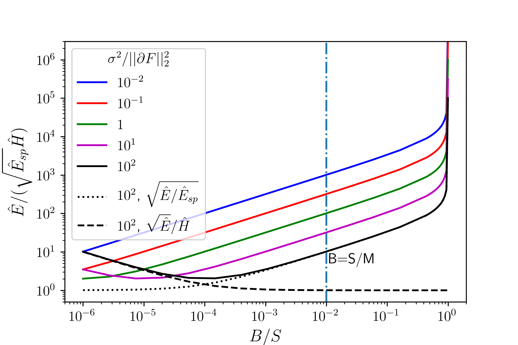
(a) $C=M$

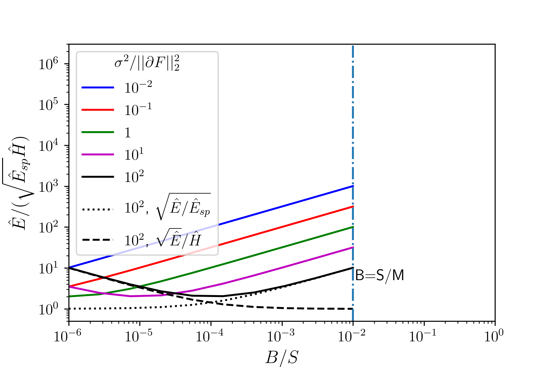
(b) $C=1$

Figure 1: Estimate of $E/(\sqrt{E_{\textrm{sp}}}H)$ versus the relative batch size $B/S$ for $M=100$, $S=10^{6}$ and different level of heterogeneity.

Figure 1 illustrates the ratio $\widehat{E}/(\sqrt{\widehat{E}_{\textrm{sp}}}\widehat{H})(=\beta\alpha)$ for a particular setting. It also highlights the two regimes discussed above: $\beta\approx 1/\alpha\times\sqrt{E/E_{\textrm{sp}}}$ for large batch sizes and $\beta\approx 1/\alpha\times\sqrt{E}/H$ for small ones. As $\beta$ indicates how much looser bound (8) is in comparison to bound (7), and $\beta>E/(\sqrt{E_{\textrm{sp}}}H)$, the figure shows that (8) may indeed overestimate the effect of the topology by many orders of magnitudes. The comparison of Fig. 1(b) and Fig. 1(a) shows that $\frac{E}{\sqrt{E_{\textrm{sp}}}H}$ (and then $\beta$) does not depend much on the replication factor $C$, but for the fact that the batch size can scale up to $CS/M$.

4 EXPERIMENTS

Table 1: Empirical estimation of $E$, $E_{\textrm{sp}}$, $H$, $\alpha$ on different ML problems and comparison of their joint effect ($\beta$) with the value $\widehat{\beta}$ predicted through (12). Number of iterations by which training losses for the ring and the clique differ by $4\%$, $10\%$, as predicted by the old bound (8), $k^{\prime}_{o}$, by the new one (7), $k^{\prime}_{n}$, and as measured in the experiment, $k^{\prime}$. When a value exceeds the total number of iterations we ran (respectively 1200 for CT, 1190 for MNIST, and 1040 for CIFAR-10), we simply indicate it as $\infty$.

Dataset	Model	M	B	$\eta$	$\sqrt{E/E_{sp}}$	$\sqrt{E}/H$	$\frac{1}{\alpha}$	$\beta$	$\widehat{\beta}$	$@4\%$			$@10\%$
										$k^{\prime}_{o}$	$k^{\prime}_{n}$	$k^{\prime}$	$k^{\prime}_{o}$	$k^{\prime}_{n}$	$k^{\prime}$
CT (S=52000)	Linear regr. n=384	16	128	0.0003	7.92	1.01	1.53	12.23	12.31	1	$\infty$	$\infty$	1	$\infty$	$\infty$
			3250		38.45	1.00	1.64	62.86	60.97	1	$\infty$	$\infty$	1	$\infty$	$\infty$
		100	128		7.75	1.01	1.54	12.05	11.56	1	10	$\infty$	1	$\infty$	$\infty$
			520		15.58	1.00	1.51	23.60	22.96	1	17	$\infty$	1	$\infty$	$\infty$
MNIST (S=60000)	2-conv layers n=431080	16	128	0.1	1.45	1.42	1.49	3.07	2.92	1	16	$\infty$	1	72	$\infty$
			500		2.15	1.14	1.53	3.75	3.71	1	22	40	1	260	$\infty$
		64	128		1.41	1.42	1.51	3.02	3.03	1	10	$\infty$	1	24	$\infty$
split by digit		10	500	0.01	1.01	1.00	1.42	1.42	3.62	1	3	60	1	7	100
CIFAR-10 (S= 50000)	ResNet18 n=11173962	16	128	0.05	1.07	3.35	1.49	5.34	5.62	1	10	30	1	20	$\infty$
			500		1.18	1.91	1.50	3.40	3.52	1	21	$\infty$	1	$250$	$\infty$

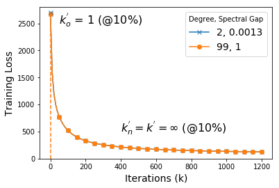
(a) CT: M=100, B = 128

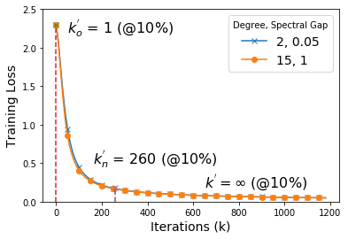
(b) MNIST: M=16, B = 500

(c) CIFAR-10: M=16, B = 500

Figure 2: Effect of network connectivity (degree $d$) on the iterations to convergence.

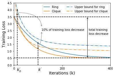
Figure 3: How to determine the number of iteration at which training loss for the clique and for the ring differs significantly.

With our experiments we want to 1) evaluate the effect of topology on the number of epochs to converge, and in particular quantify $E$, $E_{\textrm{sp}}$, $H$, and $\alpha$ in practical ML problems, 2) evaluate the effect of topology on the convergence time. We considered three different optimization problems:

1. Minimization of mean squared error (MSE) for linear regression on the dataset “Relative location of CT slices on axial axis” from (uci, ; Graf et al., 2011). Convexity holds, but gradients are potentially unbounded.

2. Minimization of cross-entropy loss through a neural network with two convolutional layers on MNIST dataset (Lecun et al., 1998). Neither convexity, nor subgradient boundness hold.

3. Minimization of cross-entropy loss through ResNet18 neural network (He et al., 2016) on CIFAR-10 dataset (Krizhevsky, 2009). Neither convexity, nor subgradient boundness hold. Moreover, we employ local subgradients with classical momentum (Sutskever et al., 2013) (with coefficient 0.9).

We have developed an ad-hoc Python simulator that allows us to test clusters with a large number of nodes, as well as a distributed application using PyTorch MPI backend to run experiments on a real GPU cluster platform. In general, datasets have been randomly split across the different workers without any replication ($C=1$). For MNIST we have also considered a scenario with $M=10$ workers, where each worker has been assigned all images for a specific digit. A constant learning rate has been set using the configuration rule from (Smith, 2017) described in Appendix G. Interestingly, for a given ML problem, when the dataset is split randomly, this procedure has led to choose the learning rate independently of the average node degree. The values selected are indicated in Table 1. Each node starts from the same model parameters ($R_{\textrm{sp}}{}=0$) that have been initialized through PyTorch default functions. We report here a subset of all results, the others can be found in Appendix G.

Table 1 shows values of $\sqrt{E/E_{\textrm{sp}}}$, $\sqrt{E}/H$, $1/\alpha$, and their product $\beta$ for different problems and different settings. $E$, $E_{\textrm{sp}}$, and $H$ have been evaluated through empirical averages using the random minibatches drawn at the first iteration. $\alpha$ is computed for an undirected ring topology. Remember that the value $\beta$ (defined in (10)) indicates how much tighter the new bound (7) is in comparison to the classic one (8). We also use (12) to provide an estimate of $\beta$ as follows $\widehat{\beta}=1/\alpha\times\widehat{E}/(\sqrt{\widehat{E}_{\textrm{sp}}}\widehat{H})$. The approximation is very accurate when the dataset is split randomly across the nodes. On the other hand, for MNIST, when all images for a given digit are assigned to the same node, local datasets are very different and approximations (12) are too crude (but our bound (7) still holds). Interestingly, $\beta$ is dominated by different effects for the three ML problems. The similarity of local datasets prevails for CT (large $\sqrt{E/E_{\textrm{sp}}}$), while the noise of stochastic subgradients prevails for CIFAR (large $\sqrt{E}/H$). For MNIST the three effects, including energy spreading over different eigenspaces ($1/\alpha$), contribute almost equally. This can be explained considering that, even if local datasets have similar sizes, they are statistically more different the more complex the model to train, i.e., the larger $n$.

From (7) and (8), we can also compute at which iteration the two bounds predict that the effect of the topology becomes significant, by identifying when the training loss difference between the clique and the ring accounts for a given percentage of the loss decrease over the entire training period. Figure 3 qualitatively illustrates the procedure. These predictions are indicated in the last columns of Table 1 and are compared with the values observed in the experiments ($k^{\prime}$).

We note that forecasts are very different, despite the fact that, in some settings, our bound is only 3 times tighter than the classic one. Bound (8) predicts that the training loss curves should differ by more than $10\%$ since the first iteration ($k^{\prime}_{o}=1$). The new bound (7) correctly identifies that the topology’s effect becomes evident later, sometimes beyond the total number of iterations performed in the experiment (in this case we indicate $k^{\prime}_{n}=\infty$).

Figure 2 shows the training loss evolution $F(\hat{\overline{\bm{w}}}(k))$ for specific settings (one for each ML problem) and two very different topologies (undirected ring and clique), when the dataset is split randomly across the nodes. The behaviour is qualitatively similar to what observed in previous works (Lian et al., 2017, 2018; Luo et al., 2019); despite the remarkable difference in the level of connectivity (quantified also by the spectral gap), the curves are very close, sometimes indistinguishable.

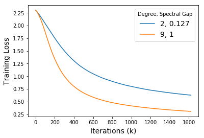
Figure 4: MNIST split by digit, M=10, B=500.

Figure 4 shows the same plot for the case when MNIST images for the same digit have been assigned to the same node. In this case the local datasets are very different and $\sqrt{E/E_{\textrm{sp}}}\approx 1$; the topology has a remarkable effect! This plot warns against extending the empirical finding in (Lian et al., 2017, 2018; Luo et al., 2019) to settings where local datasets can be highly different as it can be for example in the case of federated learning (Konecný et al., 2015).

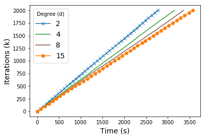
(a) Throughput

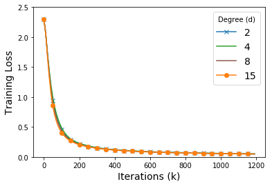
(b) Error vs iterations

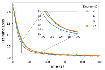
(c) Error vs time

Figure 5: Effect of network connectivity (degree $d$) on the convergence for dataset MNIST with computation times from a Spark cluster. M = 16, B = 500.

The experiments above confirm that the communication topology has little influence on the number of epochs needed to converge (when local datasets are statistically similar). Our analysis reconciles (at least in part) theory and experiments by pushing farther the training epoch at which the effect of the topology should be evident.

The conclusion about the role of the topology is radically different if one considers the time to converge. For example, Karakus et al. (2017) and Luo et al. (2019) observe experimentally that sparse topologies can effectively reduce the convergence wall-clock time. A possible explanation is that each iteration is faster because less time is spent in the communication phase: the less connected the graph, the smaller the communication load at each node. Lian et al. (2017, 2018) advance this explanation to justify why DSM on ring-like topologies can converge faster than the centralized PS.

Here, we show that sparse topologies can speed-up wall-clock time convergence even when communication costs are negligible, because they intrinsically mitigate the effect of stragglers, i.e., tasks whose completion time can be occasionally much longer than its typical value. Transient slowdowns are common in computing systems (especially in shared ones) and have many causes, such as resource contention, background OS activities, garbage collection, and (for ML tasks) stopping criteria calculations. Stragglers can significantly reduce computation speed in a multi-machine setting (Ananthanarayanan et al., 2013; Karakus et al., 2017; Li et al., 2018). For consensus-based method, one can hope that, when the topology is sparse, a temporary straggler only slows down a limited number of nodes (its out-neighbors in $\mathcal{G}$), so that the system can still maintain a high throughput.

Neglia et al. (2019) have proposed approximate formulas to evaluate the throughput of distributed ML systems for some specific random distribution of the computation time (uniform, exponential, and Pareto). Here, we take a more practical approach. Our PyTorch-based distributed application allow us to simulate systems with arbitrary distributions of the computation times and communication delays. We have carried out experiments with zero communication delays (an ideal network) and two different empirical distributions for the computation time. One was obtained by running stochastic gradient descent on a production Spark cluster with sixteen servers using Zoe Analytics (Pace et al., 2017), each with two 8-core Intel E5-2630 CPUs running at 2.40GHz. The other was extracted from ASCI-Q super-computer traces (Petrini et al., 2003, Fig. 4). Figure 5 shows the effect of topology connectivity on the convergence time for a MNIST experiment with Spark computation distribution. We consider in this case undirected $d$-regular random graphs. The number of iterations completed per node grows faster the less connected the topology (Fig. 5 (a)). As the training loss is almost independent of the topology (Fig. 5 (b)), the ring achieves the shortest convergence time (Fig. 5 (c)), even if there is no communication delay. Qualitatively similar results for other ML problems and time distributions are in Appendix G.

5 CONCLUSIONS

We have explained, both through analysis and experiments, when and why the communication topology does not affect the number of epochs consensus-based optimization methods need to converge, an effect recently observed in many papers, but not thoroughly investigated. We have also shown that, as a consequence of this invariance, a less connected topology achieves a shorter convergence time, not necessarily because it incurs a smaller communication load, but because it mitigates the stragglers’ problem. The distributed operation of consensus-based approaches appears particularly suited for federated and multi-agent learning. Our study points out that further research is required for these applications, because the benefits observed until now are dependent on the statistical similarity of the local datasets, an assumption that is not satisfied in federated learning.

6 ACKNOWLEDGEMENTS

We warmly thank Alain Jean-Marie, Pietro Michiardi, and Bruno Ribeiro for their feedback on the manuscript and their help preparing the rebuttal letter. We are also grateful to the OPAL infrastructure from Université Côte d’Azur and Inria Sophia Antipolis - Méditerranée “NEF” computation platform for providing resources and support. Finally, We would like to thank the anonymous reviewers for their insightful comments and suggestions, which helped us improve this work.

This work was supported in part by ARL under Cooperative Agreement W911NF-17-2-0196.

Appendix A Notation

We use an overline to denote an average over all the nodes and a “hat” to denote the time-average. For example

$$\overline{\bm{w}}(k)=\frac{1}{M}\sum_{i=1}^{M}{\bm{w}}_{i}(k), \hat{\bm{w}}_{i}(k)=\frac{1}{k+1}\sum_{h=0}^{k}{\bm{w}}_{i}(h).$$ (13)

For a matrix, e.g., ${\bm{W}}(k)=({\bm{w}}_{1}(k),\dots\bm{w}_{M}(k))$, $\overline{\bm{W}}(k)$ denotes the matrix whose column $i$ is $\overline{\bm{w}}(k)$, i.e.,

$$\overline{\bm{W}}(k)={\bm{W}}(k){\bm{P}}({\bm{1}}),$$

where ${\bm{P}}({\bm{1}})=\frac{{\bm{1}}{\bm{1}}^{\intercal}}{M}$ is the orthogonal projector on the subspace generated by ${\bm{1}}$. $\Delta{\bm{W}}(k)$ is used to denote the difference ${\bm{W}}(k)-\overline{\bm{W}}(k)$.

Given a matrix ${\bm{A}}$, ${\bm{A}}_{i,:}$ and ${\bm{A}}_{:,j}$ denote the $i$-th row and the $j$-th column, respectively.

We use different standard matrix norms, whose definitions are reported here for completeness. Let ${\bm{A}}$ be a $I\times J$ matrix:

$$\lVert{\bm{A}}\rVert_{2}=\sigma_{\max}({\bm{A}}),$$ (14)

$$\lVert{\bm{A}}\rVert_{F}=\sqrt{\sum_{1\leq i\leq I,1\leq j\leq J}|A_{i,j}|^{2}}=\sqrt{\sum_{i=1}^{\min(I,J)}\sigma_{i}^{2}({\bm{A}})},$$ (15)

where $\{\sigma_{i}({\bm{A}})\}$ are the singular values of the matrix ${\bm{A}}$ and $\sigma_{\max}({\bm{A}})$ is the largest one.

We will also consider the Frobenius inner product between matrices defined as follows

$$\langle{\bm{A}},{\bm{B}}\rangle_{F}\triangleq\sum_{i,j}A_{i,j}B_{i,j}=\operatorname{Tr}\left({\bm{A}}^{\intercal}{\bm{B}}\right)$$ (16)

All the results in Appendix D assume that the matrix ${\bm{A}}$ is irreducible, primitive, doubly stochastic, non-negative, and normal.

Appendix B Linear algebra reminders

B.1 Irreducible primitive doubly stochastic non-negative matrices

We remind some results from Perron-Frobenius theory (Meyer, 2000, Ch. 8). As our communication graph ${\mathcal{G}}=(\mathcal{V},\mathcal{E})$ is strongly connected, and $A_{i,j}>0$ whenever $(i,j)$ is an edge of ${\mathcal{G}}$, the $M\times M$ consensus matrix ${\bm{A}}$ is irreducible. Moreover, the consensus matrix has non-null diagonal elements and then it is also primitive. The spectral radius $\rho({\bm{A}})\triangleq\max_{i}|\lambda_{i}|$ is then itself a simple eigenvalue. Because ${\bm{A}}$ is also stochastic, its eigenvalue $\lambda_{1}=1$ coincides with the spectral radius ($1\leq\max|\lambda_{i}|\leq\|{\bm{A}}\|_{1}=1$).

Let ${\bm{P}}({\bm{1}})\triangleq\frac{{\bm{1}}{\bm{1}}^{\intercal}}{M}$ be the orthogonal projector on the subspace generated by the unit vector ${\bm{1}}$.

The non-zero singular values of ${\bm{A}}$ are the positive square roots of the non-zero eigenvalues of ${\bm{A}}^{\intercal}{\bm{A}}$. We observe that $({\bm{A}}-{\bm{P}}({\bm{1}}))^{\intercal}({\bm{A}}-{\bm{P}}({\bm{1}}))={\bm{A}}^{\intercal}{\bm{A}}-{\bm{P}}({\bm{1}})$. The spectrum of ${\bm{A}}^{\intercal}{\bm{A}}-{\bm{P}}({\bm{1}})$ is equal to the spectrum of ${\bm{A}}^{\intercal}{\bm{A}}$ but for one eigenvalue $1$ that is replaced by an eigenvalue $0$. It follows that $\sigma_{1}({\bm{A}}-{\bm{P}}({\bm{1}}))=\sigma_{2}({\bm{A}})$.

B.2 Normal matrices

An $M\times M$ matrix ${\bm{A}}$ is normal if ${\bm{A}}^{\intercal}{\bm{A}}={\bm{A}}{\bm{A}}^{\intercal}$. A matrix ${\bm{A}}$ is normal if and only if it is unitarily diagonalizable (Meyer, 2000, p. 547), i.e., it exists a complete orthonormal set of eigenvectors ${\bm{u}}_{1},{\bm{u}}_{2},\dots\bm{u}_{M}$ such that ${\bm{U}}^{\intercal}{\bm{A}}{\bm{U}}={\bm{D}}$, where ${\bm{D}}$ is the diagonal matrix containing the eigenvalues and ${\bm{U}}$ has the eigenvectors as columns.

Normal matrices have a spectral decomposition with orthogonal projectors (Meyer, 2000, p. 517), i.e.,

$${\bm{A}}=\sum_{q=1}^{Q}\lambda_{q}{\bm{P}}_{q},$$

where $\lambda_{1},\dots\lambda_{Q}$ are the $Q\leq M$ eigenvalues of ${\bm{A}}$, ${\bm{P}}_{i}$ is the orthogonal projector onto the nullspace of ${\bm{A}}-\lambda_{i}{\bm{I}}$ along the range of ${\bm{A}}-\lambda_{i}{\bm{I}}$, ${\bm{P}}_{i}{\bm{P}}_{j}=\mathbf{0}$ for $i\neq j$, and $\sum_{i=1}^{M}{\bm{P}}_{i}={\bm{I}}$. Because the projectors ${\bm{P}}_{i}$ are orthogonal and non null it holds ${\bm{P}}_{i}^{\intercal}={\bm{P}}_{i}$ and $||{\bm{P}}_{i}||_{2}=1$ (Meyer, 2000, p. 433). Moreover, for any vector ${\bm{x}}$ and $h\geq 0$, it holds:

$$\left\|{\bm{A}}^{h}{\bm{x}}\right\|_{2}^{2}=\sum_{q=1}^{Q}|\lambda_{q}|^{2h}\left\|{\bm{P}}_{q}{\bm{x}}\right\|_{2}^{2}.$$ (17)

Symmetric matrices as well as circulant matrices are normal. In fact, a circulant matrix is always diagonalizable by the Fourier matrix and then it is normal.

The non-zero singular values of a normal matrix ${\bm{A}}$ are the modules of its eigenvalues, i.e., $\sigma_{q}({\bm{A}})=|\lambda_{q}({\bm{A}})|$. If the matrix ${\bm{A}}$ is also imprimitive, irreducible, doubly stochastic and non-negative, it holds

$$\sigma_{1}({\bm{A}}-{\bm{P}}({\bm{1}}))=\sigma_{2}({\bm{A}})=|\lambda_{2}|<1.$$ (18)

Moreover, observe that in this case ${\bm{P}}_{1}={\bm{P}}({\bm{1}})$.

Appendix C Insensitivity quantification in previous work

Lian et al. (2017) and Pu et al. (2019) have studied the convergence of decentralized stochastic gradient method predicting topology independence after a certain number of iterations. Here, we evaluate quantitatively their predictions on some ML problems and compare them with our experimental observations. The results show that these predictions are very loose and then they do not fully explain why insensitivity is often observed since the beginning of the training phase.

These two papers have slightly different assumptions than ours.

A^′1

the consensus matrix ${\bm{A}}$ is symmetric and doubly stochastic,

A^′2

every $F_{j}({\bm{w}})$ has L-Lipschitz continuous gradient, i.e.,

$$\lVert\nabla F_{j}({\bm{w}})-\nabla F_{j}({\bm{v}})\rVert_{2}\leq L\lVert{\bm{w}}-{\bm{v}}\rVert_{2},\,\,\,\forall{\bm{w}},{\bm{v}}\in\mathbb{R}^{n},\forall j\in\{1,2,...,M\},$$

A^′3

the expected variance of stochastic gradient is uniformly bounded, i.e.,

$$\mathbb{E}_{\xi}[\lVert{\bm{g}}_{j}({\bm{w}})-\nabla F_{j}({\bm{w}})\rVert_{2}^{2}]\leq\sigma^{2},\,\,\,\forall{\bm{w}}\in\mathbb{R}^{n},\forall j\in\{1,2,...,M\},$$

A^′4

every $F_{j}({\bm{w}})$ is $\mu$-strongly convex, i.e.,

$$(\nabla F_{j}({\bm{w}})-\nabla F_{j}({\bm{v}}))^{T}({\bm{w}}-{\bm{v}})\geq\mu\lVert{\bm{w}}-{\bm{v}}\rVert^{2}_{2},\forall{\bm{w}},{\bm{v}}\in\mathbb{R}^{n},\forall j\in\{1,2,...,M\}.$$

We observe that A^′1 implies A4, A^′2 implies A5, and A^′4 implies A1.

Next, we will present the bounds obtained in (Lian et al., 2017; Pu et al., 2019) and how we evaluate them quantitatively.

Corollary C.1 (Corollary 2 in Lian et al. (2017)).

Under assumptions A2-A3, A^′1-A^′3, and that a constant learning rate $\eta=\frac{1}{2L+\sigma\sqrt{K/M}}$ is used, the convergence rate is independent of the topology if the total number of iterations $K$ is sufficiently large, in particular if

$$K\geq K_{l}\triangleq\frac{4L^{4}M^{5}}{\sigma^{2}(f(0)+L)^{2}(1-|\lambda_{2}|)^{2}}.$$ (19)

We estimate the constants $L,\sigma^{2}$, and $K_{l}$ as follows:

Estimate of $L$:

$\widehat{L}=\max_{j}\max_{({\bm{w}},{\bm{v}})\in\Xi}\frac{\lVert\nabla F_{j}({\bm{w}})-\nabla F_{j}({\bm{v}})\rVert_{2}}{\lVert{\bm{w}}-{\bm{v}}\rVert\_2}$, where $\Xi$ is a random set of pairs of parameter vectors.

Estimate of $\sigma^{2}$:

$\widehat{\sigma^{2}}=\frac{\max_{k}\lVert\Delta G(k)\rVert_{F}^{2}}{M}=\max_{k}\frac{E_{\textrm{sp}}(k)}{M}$, as the dataset is randomly split.

Estimate of $K_{l}$:

$\widehat{K_{l}}=\frac{4\widehat{L}^{4}M^{5}}{\widehat{\sigma^{2}}(f(0)+\widehat{L})^{2}(1-|\lambda_{2}|)^{2}}$.

We observe that $\widehat{L}$ in general underestimates the Lipschitz constant $L$, and $\widehat{\sigma^{2}}$ is likely to overestimate $\sigma^{2}$. Both effects lead to underestimate $K_{l}$, that makes our conclusions stronger.

We evaluate these quantities for three machine learning problems (SUSY, CT and MNIST). The tests are done on 16 workers with batch size $B=128$ and $|\Xi|=100$. As we want to measure from which iteration there is no difference between undirected ring and clique topologies, we consider in (19) the spectral gap ($1-|\lambda_{2}|$) of the ring. The results are given in Table 2. Corollary 19 predicts that topology insensitivity should be observed starting from $10^{6}$ iterations for MNIST and even after for the other problems. On the contrary, our experiments (see Fig. 2(a) and 2(b)) show no significant effect of topology.

Dataset	$\widehat{L}$	$\widehat{\sigma^{2}}$	$\widehat{K_{l}}$
SUSY	5.03	2.82	1.0e10
CT	37.56	1953.27	9.2e11
MNIST	86.05	12.83	2.3e6

Table 2: Number of iterations after which topology-insensitivity should manifest based on (Lian et al., 2017) for three ML problems.

Theorem C.2 (Theorem (4.2) in (Pu et al., 2019)).

Under assumptions A1-A3, A^′2-A^′4, suppose $\theta>2$, learning rate $\eta(k)=\frac{\theta}{\mu(k+K_{0})}$. For all $k\geq K_{1}-K_{0}$ it holds

$$\mathbb{E}[\lVert\bar{{\bm{w}}}(k)-{\bm{w}}^{*}\rVert^{2}] \leq \frac{\theta^{2}\sigma^{2}}{(1.5\theta-1)M\mu^{2}\tilde{k}}+\frac{3\theta^{2}(1.5\theta-1)\sigma^{2}}{(1.5\theta-2)M\mu^{2}\tilde{k}^{2}}+\frac{6\theta L^{2}V}{(1.5\theta-2)M\mu^{2}\tilde{k}^{2}},$$ (20)

where ${\bm{w}}^{*}$ is the minimizer of $F(\cdot)$, $K_{0}=\left\lceil\frac{2\theta L^{2}}{\mu^{2}}\right\rceil$, $K_{1}=\left\lceil\frac{24L^{2}\theta}{(1-|\lambda_{2}|^{2})\mu^{2}}\right\rceil$, $\tilde{k}=k+K_{0}$,
$\nabla F({\bm{w}}^{*}{\bm{1}}^{\intercal})=[\nabla F_{1}({\bm{w}}^{*}),\nabla F_{2}({\bm{w}}^{*}),\dots\nabla F_{M}({\bm{w}}^{*})]$, $X=\max\{\lVert{\bm{W}}(0)-{\bm{w}}^{*}{\bm{1}}^{\intercal}\rVert^{2}_{F},\frac{9\sum_{i=1}^{M}\lVert\nabla F_{i}({\bm{w}}^{*})\rVert^{2}_{2}}{\mu^{2}}+\frac{M\sigma^{2}}{L^{2}}\}$,
$V=\max\left\{K_{1}^{2}X,\frac{8\theta^{2}|\lambda_{2}|^{2}}{\mu^{2}(1-|\lambda_{2}|^{2})}\left(\frac{4\lVert\nabla F({\bm{w}}^{*}{\bm{1}}^{\intercal})\rVert^{2}_{F}}{1-|\lambda_{2}|^{2}}+M\sigma^{2}+\frac{4ML^{2}Y}{(1-|\lambda_{2}|^{2})K_{1}}\right)\right\}$, and $Y=\frac{K_{1}X}{M}+\frac{3}{(4\theta-3)}\left(\frac{\sigma^{2}\theta^{2}}{M\mu^{2}}+\frac{\sigma^{2}|\lambda_{2}|^{2}\theta^{2}}{2\mu^{2}}\right)+\frac{12\lVert\nabla F({\bm{w}}^{*}{\bm{1}}^{\intercal})\rVert^{2}_{F}|\lambda_{2}|^{2}\theta^{2}}{(4\theta-3)M\mu^{2}(1-|\lambda_{2}|^{2})}$.

Notice that in (20), only the third term is related to the topology as $V$ depends on the spectral gap of the consensus matrix. The bound in Corollary 19 is obtained imposing that the term depending on the spectral gap is smaller than the other terms (Lian et al., 2017, Thm. 1). Here we apply the same idea, requiring the third term of (20) to be bounded by the first and the second term of (20), i.e.,

$$\frac{6\theta L^{2}V}{(1.5\theta-2)M\mu^{2}\tilde{k}^{2}}\leq\frac{\theta^{2}\sigma^{2}}{(1.5\theta-1)M\mu^{2}\tilde{k}}+\frac{3\theta^{2}(1.5\theta-1)\sigma^{2}}{(1.5\theta-2)M\mu^{2}\tilde{k}^{2}},$$

and then

$$\frac{6L^{2}V}{(1.5\theta-2)\tilde{k}}\leq\frac{\theta\sigma^{2}}{(1.5\theta-1)}+\frac{3\theta(1.5\theta-1)\sigma^{2}}{(1.5\theta-2)\tilde{k}}.$$

Then, we have

$$\tilde{k}\geq\left(\frac{6L^{2}V}{\theta\sigma^{2}}-4.5\theta+3\right)\frac{1.5\theta-1}{1.5\theta-2}.$$

As $V\geq\left(\frac{24L^{2}\theta}{(1-|\lambda_{2}|^{2})\mu^{2}}\right)^{2}\frac{M\sigma^{2}}{L^{2}}$ and $\theta>2$, assuming that $\frac{3456ML^{4}}{\mu^{4}(1-|\lambda_{2}|^{2})^{2}}-\frac{2L^{2}}{\mu^{2}}-4.5>0$, we conclude that the convergence rate is independent of the topology if the total number of iterations $k$ is sufficiently large, and more precisely if

$$k \geq \left[\left(\frac{3456ML^{4}}{\mu^{4}(1-|\lambda_{2}|^{2})^{2}}-4.5\right)\theta+3\right]\frac{1.5\theta-1}{1.5\theta-2}-K_{0}$$

$$> \left[\left(\frac{3456ML^{4}}{\mu^{4}(1-|\lambda_{2}|^{2})^{2}}-4.5\right)\theta+3\right]-\frac{2\theta L^{2}}{\mu^{2}}-1$$

$$= \left(\frac{3456ML^{4}}{\mu^{4}(1-|\lambda_{2}|^{2})^{2}}-\frac{2L^{2}}{\mu^{2}}-4.5\right)\theta+2$$

$$> \frac{6912ML^{4}}{\mu^{4}(1-|\lambda_{2}|^{2})^{2}}-\frac{4L^{2}}{\mu^{2}}-7.$$

We denote the last expression in the sequence of inequalities as $K^{\prime}_{l}$, i.e.,

$$K^{\prime}_{l}\triangleq\frac{6912ML^{4}}{\mu^{4}(1-|\lambda_{2}|^{2})^{2}}-\frac{4L^{2}}{\mu^{2}}-7.$$ (21)

Here we evaluate $K^{\prime}_{l}$ for SUSY dataset, as its loss function is strongly convex fulfilling the assumptions of Thm. C.2. Remind that the loss function of SUSY is the hinge loss with L2 regularization $\frac{\mu}{2}\lVert{\bm{w}}\rVert^{2}$, which is $\mu$-strongly convex.

The quantity $L$ in (21) is estimated as above. We derive estimates for $K^{\prime}_{l}$, $K_{0}$, $K_{1}$ and the rule to set the learning rate $\eta(k)$, by simply replacing $\widehat{L}$ in their analytical expressions.

$\mu$	$\widehat{L}$	$\widehat{K_{0}}$	$\widehat{K_{1}}$	$\eta(0)$	$\widehat{K^{\prime}_{l}}$
0.01	5.03	2.5e6	3.1e8	2e-4	7.4e17
1	5.03	254	31140	0.02	7.4e9

Table 3: Number of iterations after which topology-insensitivity should manifest based on (Pu et al., 2019) for SUSY dataset.

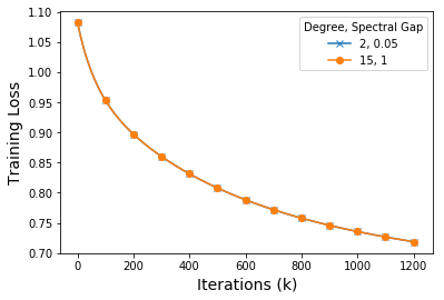
Figure 6: SUSY, M = 16, B = 128.

In our experiments, we consider $M=16$, $B=128$. As the value of $K^{\prime}_{l}$ is highly sensitive to $\mu$, we consider both $\mu=0.01$ and $\mu=1$. The results are shown in Table 3. $\widehat{K_{0}}$, $\widehat{K_{1}}$ and $\eta(0)$ are measured for the case where $\theta=5$.

The values predicted for $K^{\prime}_{l}$ are larger than 1e9 iterations. But again we observe no effect of topology in our experiments. For example, Fig. 6 shows the training loss over the number of iterations for $\mu=1$.

Appendix D Convergence results

All the following results assume that the matrix ${\bm{A}}$ is irreducible, primitive, doubly stochastic, non-negative, and normal.

Lemma D.1.

The following inequality holds.

$$\operatorname{\mathbb{E}}_{\bm{\xi}}\left[||\Delta{\bm{W}}(k+1)||_{F}\right]\leq\sqrt{M}\left\lVert\Delta{\bm{W}}(0)\right\rVert_{F}|\lambda_{2}|^{k+1}+\sum_{h=0}^{k}\eta(h)\sqrt{\sum_{l=2}^{Q}|\lambda_{l}|^{2(k-h)}\operatorname{\mathbb{E}}_{\bm{\xi}}\left[\left\lVert\Delta{\bm{G}}(h){\bm{P}}_{l}\right\rVert_{F}^{2}\right]}.$$ (22)

Proof.

$$\lVert\Delta{\bm{W}}(k+1)\rVert_{F} =\left\|{\bm{W}}(0)\left({\bm{A}}^{k+1}-{\bm{P}}({\bm{1}})\right)-\sum_{h=0}^{k}\eta(h){\bm{G}}(h)\left({\bm{A}}^{k-h}-{\bm{P}}({\bm{1}})\right)\right\|_{F}$$ (23)

$$=\left\|\Delta{\bm{W}}(0)\left({\bm{A}}^{k+1}-{\bm{P}}({\bm{1}})\right)-\sum_{h=0}^{k}\eta(h)\Delta{\bm{G}}(h)\left({\bm{A}}^{k-h}-{\bm{P}}({\bm{1}})\right)\right\|_{F}$$ (24)

$$\leq\left\|\Delta{\bm{W}}(0)\left({\bm{A}}^{k+1}-{\bm{P}}({\bm{1}})\right)\right\|_{F}+\sum_{h=0}^{k}\eta(h)\left\|\Delta{\bm{G}}(h)\left({\bm{A}}^{k-h}-{\bm{P}}({\bm{1}})\right)\right\|_{F}$$ (25)

$$=\left\|\Delta{\bm{W}}(0)\left({\bm{A}}-{\bm{P}}({\bm{1}})\right)^{k+1}\right\|_{F}+\sum_{h=0}^{k}\eta(h)\left\|\Delta{\bm{G}}(h)\left({\bm{A}}-{\bm{P}}({\bm{1}})\right)^{k-h}\right\|_{F}$$ (26)

$$=\left\|\Delta{\bm{W}}(0)(\Delta{\bm{A}})^{k+1}\right\|_{F}+\sum_{h=0}^{k}\eta(h)\left\|\Delta{\bm{G}}(h)(\Delta{\bm{A}})^{k-h}\right\|_{F}.$$ (27)

The first equality (23) follows from (5), $\overline{\bm{W}}(k+1)={\bm{W}}(k+1){\bm{P}}({\bm{1}})$, and ${\bm{A}}{\bm{P}}({\bm{1}})={\bm{P}}({\bm{1}})$, because ${\bm{A}}$ is row stochastic. Equation (24) follows from the fact that, for any matrix ${\bm{B}}$, $\overline{\bm{B}}={\bm{B}}{\bm{P}}({\bm{1}})$ and then $\overline{\bm{B}}({\bm{A}}^{h}-{\bm{P}}({\bm{1}}))={\bm{B}}{\bm{P}}({\bm{1}}){\bm{A}}^{h}-{\bm{B}}{\bm{P}}({\bm{1}})^{2}={\bm{B}}{\bm{P}}({\bm{1}})-{\bm{B}}{\bm{P}}({\bm{1}})=\mathbf{0}$, because ${\bm{A}}$ is column stochastic and ${\bm{P}}({\bm{1}})$ is a projector. For (26) expand $({\bm{A}}-{\bm{P}}({\bm{1}}))^{h}$ taking into account again that ${\bm{A}}$ is row stochastic.

Let us now bound separately the two terms on the right hand side of inequality (26). For the first one it holds

$$\left\|\Delta{\bm{W}}(0)(\Delta{\bm{A}})^{k+1}\right\|_{F} \leq\left\lVert\Delta{\bm{W}}(0)\right\rVert_{F}\left\lVert(\Delta{\bm{A}})^{k+1}\right\rVert_{F}$$

$$=\left\lVert\Delta{\bm{W}}(0)\right\rVert_{F}\sqrt{\sum_{l=2}^{M}|\lambda_{l}|^{2(k+1)}}$$

$$\leq\sqrt{M}\left\lVert\Delta{\bm{W}}(0)\right\rVert_{F}|\lambda_{2}|^{k+1},$$ (28)

where the first inequality follows from the sub-multiplicative property of Frobenius norm. For the second term on the right hand side of (26), we carry out a more careful analysis.

$$\left\lVert\Delta{\bm{G}}(h)(\Delta{\bm{A}})^{k-h}\right\rVert_{F}^{2} =\sum_{i=1}^{n}\left\lVert\Delta{\bm{G}}_{i,:}(h)(\Delta{\bm{A}})^{k-h}\right\rVert_{2}^{2}$$

$$=\sum_{i=1}^{n}\left\lVert\Delta{\bm{G}}_{i,:}(h)\sum_{l=2}^{Q}|\lambda_{l}|^{k-h}{\bm{P}}_{l}\right\rVert_{2}^{2}$$

$$=\sum_{i=1}^{n}\sum_{l=2}^{Q}|\lambda_{l}|^{2(k-h)}\left\lVert\Delta{\bm{G}}_{i,:}(h){\bm{P}}_{l}\right\rVert_{2}^{2}$$

$$=\sum_{l=2}^{Q}|\lambda_{l}|^{2(k-h)}\sum_{i=1}^{n}\left\lVert\Delta{\bm{G}}_{i,:}(h){\bm{P}}_{l}\right\rVert_{2}^{2}$$

$$=\sum_{l=2}^{Q}|\lambda_{l}|^{2(k-h)}\left\lVert\Delta{\bm{G}}(h){\bm{P}}_{l}\right\rVert_{F}^{2}.$$ (29)

From (26), (28), (29), and Jensen’s inequality, it follows

$$\operatorname{\mathbb{E}}_{\bm{\xi}}\left[||\Delta{\bm{W}}(k+1)||_{F}\right]\leq\sqrt{M}\left\lVert\Delta{\bm{W}}(0)\right\rVert_{F}|\lambda_{2}|^{k+1}+\sum_{h=0}^{k}\eta(h)\sqrt{\sum_{l=2}^{Q}|\lambda_{l}|^{2(k-h)}\operatorname{\mathbb{E}}_{\bm{\xi}}\left[\left\lVert\Delta{\bm{G}}(h){\bm{P}}_{l}\right\rVert_{F}^{2}\right]}.$$

∎

Let $R$ be a bound on the energy of the initial parameter vector across the different nodes, i.e., $\left\lVert{\bm{W}}(0)\right\rVert_{F}^{2}\leq R$, and $R_{\textrm{sp}}$ be the corresponding bound for the spread of the parameter vectors around their averages, i.e., $\left\lVert{\bm{W}}(0)-\overline{\bm{W}}(0)\right\rVert_{F}^{2}\leq R_{\textrm{sp}}$. Similarly, we define $E$ and $E_{\textrm{sp}}$ as bounds for the subgradient matrix $\Delta G$ for any time $h$: $\sup_{h\geq 0}\operatorname{\mathbb{E}}_{\bm{\xi}}\left[\left\lVert{\bm{G}}(h)\right\rVert_{F}^{2}\right]\leq E$, $\sup_{h\geq 0}\operatorname{\mathbb{E}}_{\bm{\xi}}\left[\left\lVert\Delta{\bm{G}}(h)\right\rVert_{F}^{2}\right]\leq E_{\textrm{sp}}$. We observe that $R_{\textrm{sp}}\leq R$ and $E_{\textrm{sp}}\leq E$.

Moreover, for a normal matrix ${\bm{A}}$, we define for $l=1,\dots M$:

$$E_{\textrm{sp},l}\triangleq\sup_{h\geq 0}\operatorname{\mathbb{E}}_{\bm{\xi}}\left[\left\lVert\Delta{\bm{G}}_{i,:}(h)\sum_{l^{\prime}=2}^{l}{\bm{P}}_{l^{\prime}}\right\rVert_{F}^{2}\right],$$

with the usual convention that $\sum_{i}^{j}\cdot=0$ if $j<1$ and then $E_{\textrm{sp},1}=0$. We observe that $E_{\textrm{sp},l}$ represents the maximum expected energy $\Delta{\bm{G}}(h)$ in the projection subspace defined by the first $l$ projectors. In particular it holds

$$E_{\textrm{sp},M} =\sup_{h\geq 0}\left\lVert\Delta{\bm{G}}(h)\sum_{l^{\prime}=2}^{M}{\bm{P}}_{l^{\prime}}\right\rVert_{F}^{2}=\sup_{h\geq 0}\left\lVert\Delta{\bm{G}}(h)({\bm{I}}-{\bm{P}}_{1})\right\rVert_{F}^{2}$$ (30)

$$=\sup_{h\geq 0}\left\lVert\Delta{\bm{G}}(h)\right\rVert_{F}^{2}\leq E_{\textrm{sp}}.$$ (31)

Let us now consider the normalized fraction of energy in each subspace, defined as follows:

$$e_{l} \triangleq\frac{E_{\textrm{sp},l}-E_{\textrm{sp},l-1}}{E_{\textrm{sp},M}},$$ (32)

so that $\sum_{l}e_{l}=1$. Finally, let

$$\alpha(h) \triangleq\sqrt{\sum_{l=2}^{M}e_{l}\left|\frac{\lambda_{l}}{\lambda_{2}}\right|^{2h}},$$ (33)

and we denote $\alpha(1)$ simply as $\alpha$. We observe that $|\lambda_{l}/\lambda_{2}|\leq 1$, then $\alpha(h)$ is decreasing in $h$. Moreover, $e_{2}\leq 1$ as

$$\sqrt{e_{2}}=\sqrt{e_{2}\left|\frac{\lambda_{2}}{\lambda_{2}}\right|^{2h}}\leq\sqrt{\sum_{l=2}^{M}e_{l}\left|\frac{\lambda_{l}}{\lambda_{2}}\right|^{2h}}\leq\sqrt{\sum_{l=2}^{M}e_{l}}=1.$$

$\alpha(h)$ can be considered a bound for the effective energy contribution of the vector $\Delta{\bm{G}}(h)$ in the projection subspace defined by ${\bm{P}}_{2}$.

Corollary D.2.

Considering the definition of $R_{\textrm{sp}}$, $E_{\textrm{sp}}$, and $\alpha(l)$, the following inequality holds for a constant learning rate $\eta$:

$$||\Delta{\bm{W}}(k)||_{F}\leq\sqrt{M}\sqrt{R_{\textrm{sp}}}|\lambda_{2}|^{k}+\eta\sqrt{E_{\textrm{sp}}}\left((1-\alpha)\mathbbm{1}_{k\geq 1}+\alpha\frac{1-|\lambda_{2}|^{k}}{1-|\lambda_{2}|}\right).$$ (34)

Proof.

The first term on the right hand side bounds $\sqrt{M}\left\lVert{\bm{W}}(0)\right\rVert_{F}$ by definition of $R_{\textrm{sp}}$.

Observe that

$$\sqrt{\sum_{l=2}^{M}|\lambda_{l}|^{2(k-h)}\operatorname{\mathbb{E}}_{\bm{\xi}}\left[\left\lVert\Delta{\bm{G}}(h){\bm{P}}_{l}\right\rVert_{F}^{2}\right]} \leq|\lambda_{2}|^{k-h}\sqrt{E_{\textrm{sp}}}\sqrt{\sum_{l=2}^{M}\frac{\operatorname{\mathbb{E}}_{\bm{\xi}}\left[\left\lVert\Delta{\bm{G}}(h){\bm{P}}_{l}\right\rVert_{F}^{2}\right]}{E_{\textrm{sp}}}\left|\frac{\lambda_{l}}{\lambda_{2}}\right|^{2(k-h)}}$$ (35)

$$\leq|\lambda_{2}|^{k-h}\sqrt{E_{\textrm{sp}}}\sqrt{\sum_{l=2}^{M}e_{l}\left|\frac{\lambda_{l}}{\lambda_{2}}\right|^{2(k-h)}}$$ (36)

$$\leq|\lambda_{2}|^{k-h}\sqrt{E_{\textrm{sp}}}\alpha(k-h).$$ (37)

Using this bound, we obtain

$$\sum_{h=0}^{k}\sqrt{\sum_{l=2}^{M}|\lambda_{l}|^{2(k-h)}\operatorname{\mathbb{E}}_{\bm{\xi}}\left[\left\lVert\Delta{\bm{G}}(h){\bm{P}}_{l}\right\rVert_{2}^{2}\right]} \leq\sqrt{E_{\textrm{sp}}}\sum_{h=0}^{k}\alpha(h)|\lambda_{2}|^{h}$$ (38)

$$=\sqrt{E_{\textrm{sp}}}\left(1+\sum_{h=1}^{k}\alpha(h)|\lambda_{2}|^{h}\right)$$ (39)

$$\leq\sqrt{E_{\textrm{sp}}}\left(1+\alpha(1)\sum_{h=1}^{k}|\lambda_{2}|^{h}\right)$$ (40)

$$=\sqrt{E_{\textrm{sp}}}\left(1+\alpha\sum_{h=1}^{k}|\lambda_{2}|^{h}\right)$$ (41)

$$=\sqrt{E_{\textrm{sp}}}\left((1-\alpha)+\alpha\sum_{h=0}^{k}|\lambda_{2}|^{h}\right)$$ (42)

$$=\sqrt{E_{\textrm{sp}}}\left((1-\alpha)+\alpha\frac{1-|\lambda_{2}|^{k+1}}{1-|\lambda_{2}|}\right).$$ (43)

From this last bound and (22), an inequality similar to (34), but without the indicator function, follows immediately. The indicator function can be introduced because, for $k=0$, it is simply $||\Delta{\bm{W}}(k)||_{F}\leq\sqrt{R_{\textrm{sp}}}$.

∎

Lemma D.3.

Let ${\mathbb{W}}^{*}$ the (non-empty) optimal solution set. It holds:

$$\operatorname{\mathbb{E}}_{\bm{\xi}}\left[{\operatorname{\mathrm{dist}}{\!\left(\overline{\bm{w}}(k+1),{\mathbb{W}}^{*}\right)}}^{2}\right]\leq\operatorname{\mathbb{E}}_{\bm{\xi}}\left[{\operatorname{\mathrm{dist}}{\!\left(\overline{\bm{w}}(k),{\mathbb{W}}^{*}\right)}}^{2}\right]+\frac{\eta^{2}E}{M}+\frac{4\eta H}{M}\left\lVert\Delta{\bm{W}}(k)\right\rVert_{F}-\frac{2\eta}{M}\left(\operatorname{\mathbb{E}}_{\bm{\xi}}\left[F(\overline{\bm{w}}(k))\right]-F^{*}\right).$$ (44)

where $\operatorname{\mathrm{dist}}{\!\left({\bm{x}},{\mathbb{X}}\right)}$ denotes the distance between a vector ${\bm{x}}$ and the set ${\mathbb{X}}$.

Proof.

The proof follows closely the proof in (Nedić and Ozdaglar, 2009, Lemma 5), replacing the Euclidean norm with the Frobenius norm used in this paper.

We denote the subgradients of $F_{j}$ in ${\bm{w}}_{j}(k)$ and $\overline{\bm{w}}(k)$ simply as ${\bm{g}}_{j}(k)$ and $\tilde{\bm{g}}_{j}(k)$, respectively, i.e., ${\bm{g}}_{j}(k)={\bm{g}}_{j}({\bm{w}}_{j}(k))$ and $\tilde{\bm{g}}_{j}(k)={\bm{g}}_{j}(\overline{\bm{w}}(k))$. Let ${\bm{G}}(k)$ and $\tilde{\bm{G}}(k)$ be respectively the matrices whose columns are ${\bm{g}}_{j}(k)$ and $\tilde{\bm{g}}_{j}(k)$. Let ${\bm{x}}$ be a generic vector in $\mathbb{R}^{n}$.

$$\left\lVert\overline{\bm{w}}(k+1)-{\bm{x}}\right\rVert_{2}^{2} =\left\lVert\overline{\bm{w}}(k)-{\bm{x}}-\frac{\eta}{M}\sum_{j=1}^{M}{\bm{g}}_{j}({\bm{w}}_{j}(k))\right\rVert_{2}^{2}$$

$$=\left\lVert\overline{\bm{w}}(k)-{\bm{x}}\right\rVert_{2}^{2}+\frac{\eta^{2}}{M^{2}}\left\lVert\sum_{j=1}^{M}{\bm{g}}_{j}(k)\right\rVert_{2}^{2}-\frac{2\eta}{M}\sum_{j=1}^{M}{\bm{g}}_{j}(k)^{\intercal}(\overline{\bm{w}}(k)-{\bm{x}})$$

$$\leq\left\lVert\overline{\bm{w}}(k)-{\bm{x}}\right\rVert_{2}^{2}+\frac{\eta^{2}}{M}\left\lVert{\bm{G}}(k)\right\rVert_{F}^{2}-\frac{2\eta}{M}\sum_{j=1}^{M}{\bm{g}}_{j}(k)^{\intercal}(\overline{\bm{w}}(k)-{\bm{x}}).$$ (45)

Let us bound the scalar product ${\bm{g}}_{j}(k)^{\intercal}(\overline{\bm{w}}(k)-{\bm{x}})$:

$${\bm{g}}_{j}(k)^{\intercal}(\overline{\bm{w}}(k)-{\bm{x}}) ={\bm{g}}_{j}(k)^{\intercal}(\overline{\bm{w}}(k)-{\bm{w}}_{j}(k))+{\bm{g}}_{j}(k)^{\intercal}({\bm{w}}_{j}(k)-{\bm{x}})$$

$$\geq{\bm{g}}_{j}(k)^{\intercal}(\overline{\bm{w}}(k)-{\bm{w}}_{j}(k))+F_{j}({\bm{w}}_{j}(k))-F_{j}({\bm{x}})$$ (46)

$$={\bm{g}}_{j}(k)^{\intercal}(\overline{\bm{w}}(k)-{\bm{w}}_{j}(k))+F_{j}({\bm{w}}_{j}(k))-F_{j}(\overline{\bm{w}}(k))+F_{j}(\overline{\bm{w}}(k))-F_{j}({\bm{x}})$$

$$\geq{\bm{g}}_{j}(k)^{\intercal}(\overline{\bm{w}}(k)-{\bm{w}}_{j}(k))+\tilde{\bm{g}}_{j}(k)^{\intercal}({\bm{w}}_{j}(k)-\overline{\bm{w}}(k))+F_{j}(\overline{\bm{w}}(k))-F_{j}({\bm{x}}),$$ (47)

where (46) follows from ${\bm{g}}_{j}(k)$ being a subgradient of $F_{j}$ in ${\bm{w}}_{j}(k)$ and (47) from $\tilde{\bm{g}}_{j}(k)$ being a subgradient of $F_{j}$ in $\overline{\bm{w}}(k)$. Summing over $j$ the LHS and RHS of the above inequality, we obtain:

$$\sum_{j=1}^{M}{\bm{g}}_{j}(k)^{\intercal}(\overline{\bm{w}}(k)-{\bm{x}}) \geq\sum_{j=1}^{M}{\bm{g}}_{j}(k)^{\intercal}(\overline{\bm{w}}(k)-{\bm{w}}_{j}(k))+\sum_{j=1}^{M}\tilde{\bm{g}}_{j}(k)^{\intercal}({\bm{w}}_{j}(k)-\overline{\bm{w}}(k))+\sum_{j=1}^{M}F_{j}(\overline{\bm{w}}(k))-\sum_{j=1}^{M}F_{j}({\bm{x}})$$

$$=\mathrlap{-\langle{\bm{G}}(k),\Delta{\bm{W}}(k)\rangle_{F}+\langle\tilde{\bm{G}}(k),\Delta{\bm{W}}(k)\rangle_{F}+F(\overline{\bm{w}}(k))-F({\bm{x}}),}$$

where we have used the definition of the Frobenius inner product (16). By computing the expected value we obtain

$$\operatorname{\mathbb{E}}_{\bm{\xi}}\left[\sum_{j=1}^{M}{\bm{g}}_{j}(k)^{\intercal}(\overline{\bm{w}}(k)-{\bm{x}})\right] \geq\left(\langle\operatorname{\mathbb{E}}_{\bm{\xi}}\left[{\bm{G}}(k)\right],\Delta{\bm{W}}(k)\rangle_{F}-\langle\operatorname{\mathbb{E}}_{\bm{\xi}}\left[\tilde{\bm{G}}(k)\right],\Delta{\bm{W}}(k)\rangle_{F}\right)+\operatorname{\mathbb{E}}_{\bm{\xi}}\left[F(\overline{\bm{w}}(k))-F({\bm{x}})\right]$$

$$\mathrlap{\geq-\left(\left\lVert\operatorname{\mathbb{E}}_{\bm{\xi}}\left[{\bm{G}}(k)\right]\right\rVert_{F}+\left\lVert\operatorname{\mathbb{E}}_{\bm{\xi}}\left[\tilde{\bm{G}}(k)\right]\right\rVert_{F}\right)\left\lVert\Delta{\bm{W}}(k)\right\rVert_{F}+\operatorname{\mathbb{E}}_{\bm{\xi}}\left[F(\overline{\bm{w}}(k))-F({\bm{x}})\right]}$$

$$\mathrlap{\geq-2H\left\lVert\Delta{\bm{W}}(k)\right\rVert_{F}+\operatorname{\mathbb{E}}_{\bm{\xi}}\left[F(\overline{\bm{w}}(k))-F({\bm{x}})\right]}.$$ (48)

From (45) and (48), we obtain:

$$\operatorname{\mathbb{E}}_{\bm{\xi}}\left[\left\lVert\overline{\bm{w}}(k+1)-{\bm{x}}\right\rVert_{2}^{2}\right]\leq \operatorname{\mathbb{E}}_{\bm{\xi}}\left[\left\lVert\overline{\bm{w}}(k)-{\bm{x}}\right\rVert_{2}^{2}\right]+\frac{\eta^{2}E}{M}+\frac{4\eta H}{M}\left\lVert\Delta{\bm{W}}(k)\right\rVert_{F}-\frac{2\eta}{M}\operatorname{\mathbb{E}}_{\bm{\xi}}\left[F(\overline{\bm{w}}(k))-F({\bm{x}})\right].$$ (49)

Then the thesis follows from considering ${\bm{x}}$ a generic point in the optimal set ${\mathbb{W}}^{*}$. ∎

D.1 Proof of Proposition 3.1

Proof.

We start computing a bound for the time average of $\left\lVert\Delta{\bm{W}}(k)\right\rVert_{F}$ using Corollary D.2:

$$\frac{1}{K}\sum_{k=0}^{K-1}\left\lVert\Delta{\bm{W}}(k)\right\rVert_{F}\leq \frac{\sqrt{M}\sqrt{R_{\textrm{sp}}}}{K}\frac{1-|\lambda_{2}|^{K}}{1-|\lambda_{2}|}+\eta\sqrt{E_{\textrm{sp}}}(1-\alpha)\frac{K-1}{K}$$

$$+\frac{\eta\sqrt{E_{\textrm{sp}}}\alpha}{1-|\lambda_{2}|}\left(1-\frac{1}{K}\frac{1-|\lambda_{2}|^{K}}{1-|\lambda_{2}|}\right)$$ (50)

If we take into account convexity of $F$, Lemma D.3, and (50), we obtain:

$$\operatorname{\mathbb{E}}_{\bm{\xi}}\left[F\!\left(\hat{\overline{\bm{w}}}(k)\right)\right]-F^{*} =\operatorname{\mathbb{E}}_{\bm{\xi}}\left[F\!\left(\frac{1}{K}\sum_{k=0}^{K-1}\overline{\bm{w}}(k)\right)\right]-F^{*}$$

$$\underset{\textrm{convexity}}{\leq}\frac{1}{K}\sum_{k=0}^{K-1}\left(\operatorname{\mathbb{E}}_{\bm{\xi}}\left[F(\overline{\bm{w}}(k))\right]-F^{*}\right)$$

$$\underset{\textrm{Lem~{}\ref{l:distance}}}{\leq}\frac{1}{K}\sum_{k=0}^{K-1}\left(\frac{M}{2\eta}\left({\operatorname{\mathrm{dist}}{\!\left(\overline{\bm{w}}(k),{\mathbb{W}}^{*}\right)}}^{2}-{\operatorname{\mathrm{dist}}{\!\left(\overline{\bm{w}}(k+1),{\mathbb{W}}^{*}\right)}}^{2}\right)+\frac{\eta E}{2}+2H\left\lVert\Delta{\bm{W}}(k)\right\rVert_{F}\right)$$

$$=\frac{M}{2\eta K}\left({\operatorname{\mathrm{dist}}{\!\left(\overline{\bm{w}}(0),{\mathbb{W}}^{*}\right)}}^{2}-{\operatorname{\mathrm{dist}}{\!\left(\overline{\bm{w}}(K),{\mathbb{W}}^{*}\right)}}^{2}\right)+\frac{\eta E}{2}+2H\frac{1}{K}\sum_{k=0}^{K-1}\left\lVert\Delta{\bm{W}}(k)\right\rVert_{F}$$

$$\leq\frac{M}{2\eta K}{\operatorname{\mathrm{dist}}{\!\left(\overline{\bm{w}}(0),{\mathbb{W}}^{*}\right)}}^{2}+\frac{\eta E}{2}+2H\frac{1}{K}\sum_{k=0}^{K-1}\left\lVert\Delta{\bm{W}}(k)\right\rVert_{F}$$

$$\underset{\textrm{\eqref{e:avg_frob_bound}}}{\leq}\frac{M}{2\eta K}{\operatorname{\mathrm{dist}}{\!\left(\overline{\bm{w}}(0),{\mathbb{W}}^{*}\right)}}^{2}+\frac{\eta E}{2}+2H\frac{\sqrt{M}\sqrt{R_{\textrm{sp}}}}{K}\frac{1-|\lambda_{2}|^{K}}{1-|\lambda_{2}|}$$

$$\phantom{\underset{\textrm{\eqref{e:avg_frob_bound}}}{\leq}}+2H\eta\sqrt{E_{\textrm{sp}}}\left((1-\alpha)\frac{K-1}{K}+\frac{\alpha}{1-|\lambda_{2}|}\left(1-\frac{1}{K}\frac{1-|\lambda_{2}|^{K}}{1-|\lambda_{2}|}\right)\right)$$ (51)

∎

D.2 Proof of Corollary 3.2

Proof.

Because of the relations $R_{\textrm{sp}}\leq R$ and $E_{\textrm{sp}}\leq E$, the only step to prove is that

$$(1-\alpha)\frac{K-1}{K}+\alpha\frac{1}{1-|\lambda_{2}|}\left(1-\frac{1}{K}\frac{1-|\lambda_{2}|^{K}}{1-|\lambda_{2}|}\right)\leq\frac{1}{1-|\lambda_{2}|}\left(1-\frac{1}{K}\frac{1-|\lambda_{2}|^{K}}{1-|\lambda_{2}|}\right).$$ (52)

The two sides can be rewritten as the sums indicated below:

$$\frac{1}{K}\sum_{k=0}^{K-1}\left((1-\alpha)\mathbbm{1}_{k\geq 1}+\alpha\frac{1-|\lambda_{2}|^{k}}{1-|\lambda_{2}|}\right)\leq\frac{1}{K}\sum_{k=0}^{K-1}\frac{1-|\lambda_{2}|^{k}}{1-|\lambda_{2}|}.$$ (53)

It is then sufficient to prove that for each $k\geq 0$

$$(1-\alpha)\mathbbm{1}_{k\geq 1}+\alpha\frac{1-|\lambda_{2}|^{k}}{1-|\lambda_{2}|}\leq\frac{1-|\lambda_{2}|^{k}}{1-|\lambda_{2}|}.$$ (54)

This relation is obviously satisfied for $k=0$ ($\alpha<1$). For any $k>0$, it follows from

$$\frac{1-|\lambda_{2}|^{k}}{1-|\lambda_{2}|}=\sum_{h=0}^{k-1}|\lambda_{2}|^{h}\geq 1.$$ (55)

∎

D.3 Convergence of local estimates

Proposition D.4.

Under assumptions A1-A5 and that a constant learning rate $\eta(k)=\eta$ is used, an upper bound for the objective value at the end of the ($K-1$)th iteration is given, for each $i$, by:

$$\operatorname{\mathbb{E}}\left[F\!\left(\hat{\bm{w}}_{i}(K-1)\right)\right]-F^{*}\leq \frac{M}{2\eta{K}}{\operatorname{\mathrm{dist}}{\!\left(\overline{\bm{w}}(0),{\mathbb{W}}^{*}\right)}}^{2}+\frac{\eta E}{2}+H\frac{3M\sqrt{R_{\textrm{sp}}}}{K}\frac{1-|\lambda_{2}|^{K}}{1-|\lambda_{2}|}$$

$$+3\eta\sqrt{M}H\sqrt{E_{\textrm{sp}}}\left((1-\alpha)\frac{K-1}{K}+\frac{\alpha}{1-|\lambda_{2}|}\left(1-\frac{1}{K}\frac{1-|\lambda_{2}|^{K}}{1-|\lambda_{2}|}\right)\right).$$ (56)

Proof.

We consider the local model at node $i$ (${\bm{w}}_{i}(k)$). Using convexity of the local functions and the definition of subgradients, we obtain:

$$\operatorname{\mathbb{E}}_{\bm{\xi}}\left[F\!\left(\hat{{\bm{w}}}_{i}(k)\right)\right] =\sum_{j=1}^{M}\operatorname{\mathbb{E}}_{\bm{\xi}}\left[F_{j}\!\left(\hat{{\bm{w}}}_{i}(k)\right)\right]\underset{\textrm{convexity}}{\leq}\sum_{j=1}^{M}\left(\operatorname{\mathbb{E}}_{\bm{\xi}}\left[F_{j}\!\left(\hat{\overline{\bm{w}}}(k)\right)\right]+\operatorname{\mathbb{E}}_{\bm{\xi}}\left[{\bm{g}}_{j}\!(\hat{{\bm{w}}}_{i}(k))\right]^{\intercal}(\hat{{\bm{w}}}_{i}(k)-\hat{\overline{\bm{w}}}(k))\right)$$

$$=\operatorname{\mathbb{E}}_{\bm{\xi}}\left[F\!\left(\hat{\overline{\bm{w}}}(k)\right)\right]+\sum_{j=1}^{M}\operatorname{\mathbb{E}}_{\bm{\xi}}\left[{\bm{g}}_{j}\!(\hat{{\bm{w}}}_{i}(k))\right]^{\intercal}(\hat{{\bm{w}}}_{i}(k)-\hat{\overline{\bm{w}}}(k))$$

$$\leq\operatorname{\mathbb{E}}_{\bm{\xi}}\left[F\!\left(\hat{\overline{\bm{w}}}(k)\right)\right]+\sum_{j=1}^{M}\left\lVert\operatorname{\mathbb{E}}_{\bm{\xi}}\left[{\bm{g}}_{j}\!(\hat{{\bm{w}}}_{i}(k))\right]\right\rVert_{2}\lVert\hat{{\bm{w}}}_{i}(k)-\hat{\overline{\bm{w}}}(k)\rVert_{2}$$

$$\leq\operatorname{\mathbb{E}}_{\bm{\xi}}\left[F\!\left(\hat{\overline{\bm{w}}}(k)\right)\right]+\sqrt{M}\left\lVert\operatorname{\mathbb{E}}_{\bm{\xi}}\left[G(\hat{{\bm{w}}}_{i}(k))\right]\right\rVert_{F}\left\lVert\hat{{\bm{w}}}_{i}(k)-\hat{\overline{\bm{w}}}(k)\right\rVert_{2}$$

$$\leq\operatorname{\mathbb{E}}_{\bm{\xi}}\left[F\!\left(\hat{\overline{\bm{w}}}(k)\right)\right]+\sqrt{M}H\left\lVert\hat{{\bm{w}}}_{i}(k)-\hat{\overline{\bm{w}}}(k)\right\rVert_{2}$$

$$\leq\operatorname{\mathbb{E}}_{\bm{\xi}}\left[F\!\left(\hat{\overline{\bm{w}}}(k)\right)\right]+\sqrt{M}H\frac{1}{K}\sum_{k=0}^{K-1}\lVert{\bm{w}}_{i}(k)-\overline{\bm{w}}(k)\rVert_{2}$$

$$\leq\operatorname{\mathbb{E}}_{\bm{\xi}}\left[F\!\left(\hat{\overline{\bm{w}}}(k)\right)\right]+\sqrt{M}H\frac{1}{K}\sum_{k=0}^{K-1}\left\lVert{\bm{W}}(k)-\overline{\bm{W}}(k)\right\rVert_{F}$$

$$\leq\operatorname{\mathbb{E}}_{\bm{\xi}}\left[F\!\left(\hat{\overline{\bm{w}}}(k)\right)\right]+\sqrt{M}H\frac{\sqrt{M}\sqrt{R_{\textrm{sp}}}}{K}\frac{1-|\lambda_{2}|^{K}}{1-|\lambda_{2}|}$$

$$\phantom{\leq}+\sqrt{M}H\eta\sqrt{E_{\textrm{sp}}}\left((1-\alpha)\frac{K-1}{K}+\frac{\alpha}{1-|\lambda_{2}|}\left(1-\frac{1}{K}\frac{1-|\lambda_{2}|^{K}}{1-|\lambda_{2}|}\right)\right).$$ (57)

Putting together (51) and (57), we obtain:

$$\operatorname{\mathbb{E}}_{\bm{\xi}}\left[F\!\left(\hat{{\bm{w}}}_{i}(k)\right)\right]-F^{*} \leq\frac{M}{2\eta K}{\operatorname{\mathrm{dist}}{\!\left(\overline{\bm{w}}(0),{\mathbb{W}}^{*}\right)}}^{2}+\frac{\eta E}{2}+(2+\sqrt{M})H\frac{\sqrt{M}\sqrt{R_{\textrm{sp}}}}{K}\frac{1-|\lambda_{2}|^{K}}{1-|\lambda_{2}|}$$

$$\phantom{\leq}+(2+\sqrt{M})H\eta\sqrt{E_{\textrm{sp}}}\left((1-\alpha)\frac{K-1}{K}+\frac{\alpha}{1-|\lambda_{2}|}\left(1-\frac{1}{K}\frac{1-|\lambda_{2}|^{K}}{1-|\lambda_{2}|}\right)\right)$$

$$\leq\frac{M}{2\eta K}{\operatorname{\mathrm{dist}}{\!\left(\overline{\bm{w}}(0),{\mathbb{W}}^{*}\right)}}^{2}+\frac{\eta E}{2}+H\frac{3M\sqrt{R_{\textrm{sp}}}}{K}\frac{1-|\lambda_{2}|^{K}}{1-|\lambda_{2}|}$$

$$\phantom{\leq}+3\sqrt{M}H\eta\sqrt{E_{\textrm{sp}}}\left((1-\alpha)\frac{K-1}{K}\phantom{\leq}+\frac{\alpha}{1-|\lambda_{2}|}\left(1-\frac{1}{K}\frac{1-|\lambda_{2}|^{K}}{1-|\lambda_{2}|}\right)\right),$$ (58)

where the last inequality is simply to slightly compact the formula. ∎

Corollary D.5.

Under assumptions A1-A5 and that constant learning rate $\eta(k)=\eta$ is used, an upper bound for the objective value at the end of the ($K-1$)th iteration is given, for each $i$, by:

$$\operatorname{\mathbb{E}}\left[F\!\left(\hat{\bm{w}}_{i}(K-1)\right)\right]-F^{*}\leq \frac{M}{2\eta{K}}{\operatorname{\mathrm{dist}}{\!\left(\overline{\bm{w}}(0),{\mathbb{W}}^{*}\right)}}^{2}+\frac{\eta E}{2}+\sqrt{E}\frac{3M\sqrt{R}}{K}\frac{1-|\lambda_{2}|^{K}}{1-|\lambda_{2}|}+\frac{3\eta\sqrt{M}E}{1-|\lambda_{2}|}\left(1-\frac{1}{K}\frac{1-|\lambda_{2}|^{K}}{1-|\lambda_{2}|}\right).$$ (59)

In particular, if workers compute full-batch subgradients and the 2-norm of subgradients of functions $F_{i}$ is bounded by a constant $L$, we obtain:

$$F\!\left(\hat{\bm{w}}_{i}(K-1)\right)-F^{*}\leq \frac{M}{2\eta{K}}{\operatorname{\mathrm{dist}}{\!\left(\overline{\bm{w}}(0),{\mathbb{W}}^{*}\right)}}^{2}+\frac{\eta ML^{2}}{2}+L\frac{3M^{3/2}\sqrt{R}}{K}\frac{1-|\lambda_{2}|^{K}}{1-|\lambda_{2}|}+\frac{3\eta M^{3/2}L^{2}}{1-|\lambda_{2}|}\left(1-\frac{1}{K}\frac{1-|\lambda_{2}|^{K}}{1-|\lambda_{2}|}\right).$$ (60)

Proof.

The result follows immediately from Proposition D.4 and (52). ∎

Appendix E Proof of Proposition 3.3

Proof.

Our first remark is that selecting a uniform permutation and then a uniform random batch of size $B$ without resampling is equivalent to selecting uniformly $B$ elements from the dataset ${\mathbb{S}}$ without resampling. We denote this sampling with the random variable $\xi_{\mathbb{S}}$. This is true independently from the presence of data replication, as far as data point replicas are located at different nodes. From this observation and the formula for the variance of the average of a sample drawn without resampling, it follows:

$$\operatorname{\mathbb{E}}_{\pi}\left[\operatorname{\mathbb{E}}_{\bm{\xi}}\left[\left\lVert{\bm{G}}\right\rVert_{F}^{2}\right]\right] =\sum_{i,j}\operatorname{\mathbb{E}}_{\pi}\left[\operatorname{\mathbb{E}}_{\bm{\xi}}\left[{G}_{i,j}^{2}\right]\right]=\sum_{i,j}\operatorname{\mathbb{E}}_{\xi_{{\mathbb{S}}}}\left[{G}_{i,j}^{2}\right]=\sum_{i,j}\left(\left(\operatorname{\mathbb{E}}_{\xi_{{\mathbb{S}}}}\left[{G}_{i,j}\right]\right)^{2}+\mathrm{Var}_{\xi_{{\mathbb{S}}}}\!\left[{G}_{i,j}\right]\right)$$

$$=\sum_{i,j}\left((\partial F)_{i}^{2}+\frac{S}{S-1}\frac{\sigma_{i}^{2}}{B}\left(1-\frac{B}{S}\right)\right)=\sum_{i,j}\left((\partial F)_{i}^{2}+\frac{S-B}{S-1}\frac{\sigma_{i}^{2}}{B}\right)$$

$$=M\left(\left\lVert\partial F\right\rVert_{2}^{2}+\frac{S-B}{S-1}\frac{\sigma^{2}}{B}\right).$$ (61)

From $\sum_{j=1}^{M}x_{j}^{2}=\sum_{j=1}^{M}(x_{j}-\bar{x})^{2}+M\bar{x}^{2}$, where $\bar{x}$ denote the mean of the $M$ values $x_{j}$, it follows

$$\left\lVert\Delta{\bm{G}}\right\rVert_{F}^{2} =\left\lVert{\bm{G}}\right\rVert_{F}^{2}-\left\lVert{\bm{G}}\frac{{\bm{1}}{\bm{1}}^{\intercal}}{M}\right\rVert_{F}^{2}.$$ (62)

In order to compute $\operatorname{\mathbb{E}}_{\pi}\left[\operatorname{\mathbb{E}}_{\bm{\xi}}\left[\left\lVert\Delta{\bm{G}}\right\rVert_{F}^{2}\right]\right]$, we will then compute $\operatorname{\mathbb{E}}_{\pi}\left[\operatorname{\mathbb{E}}_{\bm{\xi}}\left[\left\lVert{\bm{G}}{\bm{1}}{\bm{1}}^{\intercal}/M\right\rVert_{F}^{2}\right]\right]$ and then use (61) and (62). We denote the double expectation over $\bf\xi$ and $\pi$ simply as $\operatorname{\mathbb{E}}\left[\right]$.

$$\operatorname{\mathbb{E}}\left[\left(\frac{1}{M}\sum_{j=1}^{M}G_{i,j}\right)^{2}\right] =\frac{1}{M^{2}}\left(\sum_{j}\operatorname{\mathbb{E}}\left[G_{i,j}^{2}\right]+\sum_{j\neq j^{\prime}}^{M}\operatorname{\mathbb{E}}\left[G_{i,j}G_{i,j^{\prime}}\right]\right)$$

$$=\frac{1}{M}\left(\operatorname{\mathbb{E}}\left[G_{i,j}^{2}\right]+(M-1)\operatorname{\mathbb{E}}\left[G_{i,j}G_{i,j^{\prime}}\right]\right),$$ (63)

where $j$ and $j^{\prime}$ are arbitrary values in $\{1,\dots M\}$ with $j^{\prime}\neq j$.

$$\operatorname{\mathbb{E}}\left[G_{i,j}^{2}\right] =\operatorname{\mathbb{E}}\left[G_{i,j}\right]^{2}+\mathrm{Var}\left[G_{i,j}\right]=(\partial F)_{i}^{2}+\frac{S-B}{S-1}\frac{\sigma_{i}^{2}}{B}.$$ (64)

Let $\mathbbm{1}_{s,s^{\prime}}$ be the indicator function denoting if the datapoint $(x^{(s)},y^{(s)})$ has been selected in the minibatch at node $j$ and the datapoint $(x^{(s^{\prime})},y^{(s^{\prime})})$ has been selected in the minibatch at node $j^{\prime}$. In order to keep the notation compact we also denote by $\partial f_{i,s}$ and $\partial f_{i,s^{\prime}}$ respectively $(\partial f({\bm{w}},(x^{(s)},y^{(s)})))_{i}$ and $(\partial f({\bm{w}},(x^{(s^{\prime})},y^{(s^{\prime})})))_{i}$.

$$\operatorname{\mathbb{E}}\left[G_{i,j}G_{i,j^{\prime}}\right] =\frac{1}{B^{2}}\sum_{s=1}^{S}\sum_{s^{\prime}=1}^{S}\partial f_{i,s}\partial f_{i,s^{\prime}}\operatorname{\mathbb{E}}\left[\mathbbm{1}_{s,s^{\prime}}\right].$$ (65)

The probability that the point $s$ is in the local dataset at node $i$ and the point is selected in the minibatch is $\frac{CS/M}{S}\times\frac{B}{CS/M}=\frac{B}{S}$. Let us consider first the case $s^{\prime}=s$. Given that $s$ is in $j$, the probability that one of the other $C-1$ copies is stored in $j^{\prime}$ is $\frac{C-1}{M-1}$ and this copy has a probability $\frac{B}{CS/M}$ to be selected. Then the total probability of the event that a copy of $s$ is selected in the minibatch at $j$ and another copy is selected in the minibatch at $j^{\prime}$ is

$$\frac{B}{S}\times\frac{C-1}{M-1}\times\frac{B}{CS/M}=\frac{B^{2}}{S^{2}}\frac{C-1}{C}\frac{M}{M-1}.$$

If $s^{\prime}\neq s$, then $s^{\prime}$ may be present in $j$ or not. The first event occurs with probability $\frac{\frac{CS}{M}-1}{S-1}$ (because $s$ has already been located in $j$) and in this case the probability that $s^{\prime}$ is also located in $j^{\prime}$ is $\frac{C-1}{M-1}$. $s^{\prime}$ is not present in $j$ with probability $1-\frac{\frac{CS}{M}-1}{S-1}$ and in this case it is located in $j^{\prime}$ with probability $\frac{C}{M-1}$. Then the total probability of the event that a copy of $s^{\prime}$ is located at $j^{\prime}$ given that a copy of $s$ is located at $j$ is

$$\frac{\frac{CS}{M}-1}{S-1}\frac{C-1}{M-1}+\left(1-\frac{\frac{CS}{M}-1}{S-1}\right)\frac{C}{M-1}=\frac{C}{M}+\frac{M-C}{M(M-1)(S-1)},$$

and the probability that a copy of $s$ is selected in the minibatch at $j$ and a copy of $s^{\prime}\neq s$ is located at $j^{\prime}$ is

$$\frac{B}{S}\times\frac{C}{M}+\frac{M-C}{M(M-1)(S-1)}\times\frac{B}{\frac{CS}{M}}=\frac{B^{2}}{S^{2}}\left(1+\frac{M-C}{C(M-1)(S-1)}\right).$$

In conclusion, we have just proved that:

$$\operatorname{\mathbb{E}}\left[\mathbbm{1}_{s,s^{\prime}}\right]=\begin{cases}\frac{B^{2}}{S^{2}}\frac{C-1}{C}\frac{M}{M-1},&\textrm{ for }s^{\prime}=s,\\ \frac{B^{2}}{S^{2}}\left(1+\frac{M-C}{C(M-1)(S-1)}\right),&\textrm{ for }s^{\prime}\neq s.\end{cases}$$ (66)

We observe that

$$\frac{1}{S}\sum_{s}(\partial f_{i,s})^{2}=(\partial F)_{i}^{2}+\sigma_{i}^{2},$$ (67)

$$(\partial F)_{i}^{2}=\left(\frac{1}{S}\sum_{s}\partial f_{i,s}\right)^{2}=\frac{1}{S^{2}}\left(\sum_{s}(\partial f_{i,s})^{2}+\sum_{s\neq s^{\prime}}\partial f_{i,s}\partial f_{i,s^{\prime}}\right).$$ (68)

Using these two relations and (66) in (65) we obtain

$$\operatorname{\mathbb{E}}\left[G_{i,j}G_{i,j^{\prime}}\right] =(\partial F)_{i}^{2}+\sigma_{i}^{2}\frac{C-M}{C(M-1)(S-1)}.$$ (69)

This equality together with (63) and (64) leads to:

$$\operatorname{\mathbb{E}}\left[\left\lVert{\bm{G}}{\bm{1}}{\bm{1}}^{\intercal}/M\right\rVert_{F}^{2}\right] =\sum_{i}\operatorname{\mathbb{E}}\left[G_{i,j}^{2}\right]+(M-1)\operatorname{\mathbb{E}}\left[G_{i,j}G_{i,j^{\prime}}\right]$$

$$=\left\lVert\partial F\right\rVert_{2}^{2}+\frac{S-B}{S-1}\frac{\sigma^{2}}{B}+(M-1)\left(\left\lVert\partial F\right\rVert_{2}^{2}+\sigma^{2}\frac{C-M}{C(M-1)(S-1)}\right)$$

$$=M\left\lVert\partial F\right\rVert_{2}^{2}+\sigma_{2}\frac{CS-MB}{CB(S-1)}.$$ (70)

Finally,

$$\operatorname{\mathbb{E}}\left[\left\lVert\Delta{\bm{G}}\right\rVert_{F}^{2}\right] =\operatorname{\mathbb{E}}\left[\left\lVert{\bm{G}}\right\rVert_{F}^{2}\right]-\operatorname{\mathbb{E}}\left[\left\lVert{\bm{G}}{\bm{1}}{\bm{1}}^{\intercal}/M\right\rVert_{F}^{2}\right]$$ (71)

$$=M\sigma^{2}\left(\frac{S-B}{B(S-1)}-\frac{CS-MB}{MCB(S-1)}\right).$$ (72)

We now move to bound $\operatorname{\mathbb{E}}_{\pi}\left[\left\lVert\operatorname{\mathbb{E}}_{\bm{\xi}}\left[{\bm{G}}\right]\right\rVert_{F}\right]$. The lower bound follows immediately from the fact that any norm is a convex function, so that

$$\operatorname{\mathbb{E}}_{\pi}\left[\left\lVert\operatorname{\mathbb{E}}_{\bm{\xi}}\left[{\bm{G}}\right]\right\rVert_{F}\right]\geq\left\lVert\operatorname{\mathbb{E}}_{\pi}\left[\operatorname{\mathbb{E}}_{\bm{\xi}}\left[{\bm{G}}\right]\right]\right\rVert_{F}=\sqrt{M}\left\lVert\partial F\right\rVert_{2}.$$

For the upper bound:

$$\operatorname{\mathbb{E}}_{\pi}\left[\left\lVert\operatorname{\mathbb{E}}_{\bm{\xi}}\left[{\bm{G}}\right]\right\rVert_{F}\right] =\operatorname{\mathbb{E}}_{\pi}\left[\sqrt{\sum_{i,j}\left(\operatorname{\mathbb{E}}_{\bm{\xi}}\left[G_{i,j}\right]\right)^{2}}\right]$$

$$\leq\sqrt{\sum_{i,j}\operatorname{\mathbb{E}}_{\pi}\left[\left(\operatorname{\mathbb{E}}_{\bm{\xi}}\left[G_{i,j}\right]\right)^{2}\right]}$$ (73)

$$=\sqrt{\sum_{i,j}\left(\operatorname{\mathbb{E}}_{\pi}\left[\operatorname{\mathbb{E}}_{\bm{\xi}}\left[G_{i,j}\right]\right]\right)^{2}+\mathrm{Var}_{\pi}\left[\operatorname{\mathbb{E}}_{\bm{\xi}}\left[G_{i,j}\right]\right]}$$ (74)

$$=\sqrt{\sum_{i,j}(\partial F)_{i}^{2}+\sigma_{i}^{2}\frac{M-C}{C(S-1)}}$$ (75)

$$=\sqrt{M\left(\left\lVert\partial F\right\rVert_{2}^{2}+\frac{M-C}{C(S-1)}\sigma^{2}\right)},$$ (76)

where the first inequality follows from the concavity of square root function. Observe that $\operatorname{\mathbb{E}}_{\bm{\xi}}\left[G_{:,j}\right]$ is equal to the full-batch gradient computed on the local dataset at node $j$. As such, its expected value over the permutations $\pi$ is equal to $\partial F$, and its variance corresponds to the variance of the sample average when we draw $CS/M$ samples from a dataset of $S$ elements without resampling. ∎

Appendix F Toy example

In this section we consider a toy example to illustrate the implications of the findings in the previous section. We want to solve the following problem:

$$\operatorname*{minimize}_{w} F(w)=\frac{1}{M}\sum_{l=1}^{M}1-y^{(l)}x^{(l)}w$$ (77)

subject to $$w\in{\mathbb{W}}$$

where $x^{(l)}$ is a data feature and $y^{(l)}\in\{-1,1\}$ identifies the class label. Note that there is only one parameter $w\in\mathbb{R}$ ($n=1$) and, for the moment, the number of nodes equals the size of the dataset ($M=m$). $\Delta{\bm{G}}(k)={\bm{G}}(k)-{\bm{G}}(k)\frac{{\bm{1}}{\bm{1}}^{\intercal}}{M}$ is in this case a constant row vector.

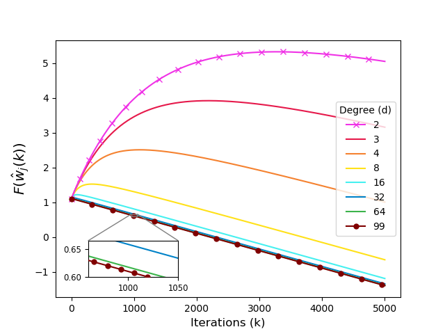
(a) Rings with aligned gradient

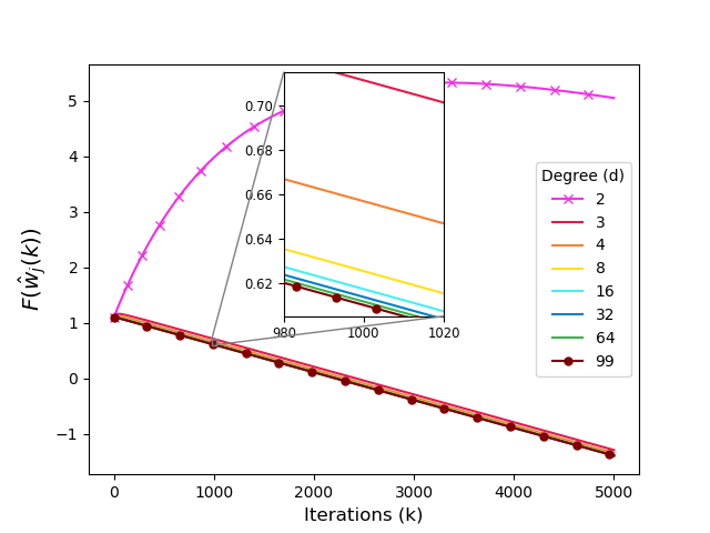
(b) Expanders with aligned gradient

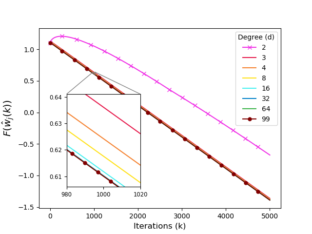
(c) Expanders with generic gradient

Figure 7: Objective function (77) evaluated for the worst model ${\bm{w}}_{j}(k)$ versus number of iterations: effect of the topology and its relation with the gradients.

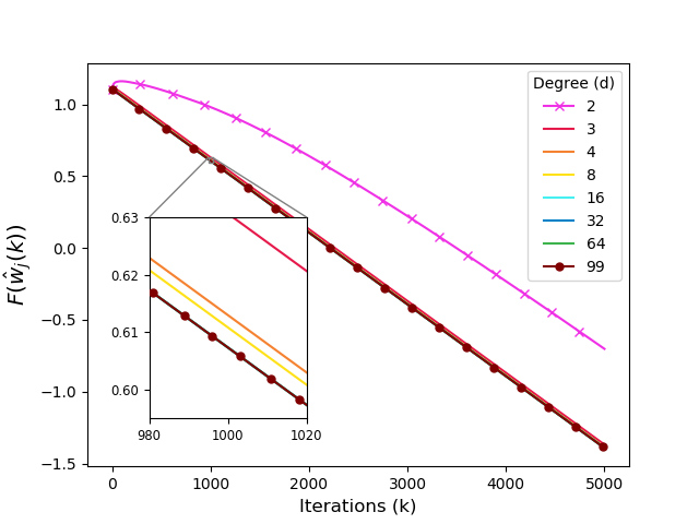
(a) 2X dataset

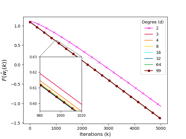
(b) 20X dataset

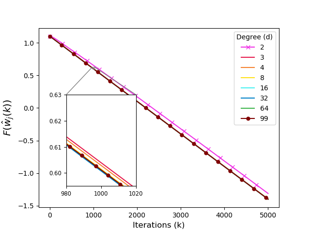
(c) 100X dataset

Figure 8: Objective function (77) evaluated for the worst model ${\bm{w}}_{j}(k)$ versus number of iterations: effect of dataset size. Expanders with generic gradient.

We consider an undirected $d$-regular graph with $M=100$ nodes and homogeneous non-negative weights, i.e., $A_{i,j}=1/(d+1)$ for $(i,j)\in\mathcal{E}$ and $A_{i,j}=0$ otherwise. Matrix ${\bm{A}}$ is then symmetric.

Figure 7(a) presents results for undirected $d$-regular rings, where each node $i$ is connected to nodes $i-1$ and $i+1$ (hence forming a cycle) as well as the $d-2$ closest nodes on the cycle. Among graphs with degree $d$, these rings are poorly connected, with a diameter that is order of $M/d$ and low spectral gap $1-|\lambda_{2}|$. The curves show the evolution of the objective function evaluated at the worst estimate, i.e., $\max_{i}F(\hat{w}_{i}(k))$ for different values of the degree $d$. For each degree, the dataset is chosen selecting a vector ${\bm{u}}$ orthogonal to ${\bm{1}}$ and perturbing each of its components by a small amount $\zeta$, so that ${\bm{G}}={\bm{u}}^{\intercal}+\zeta{\bm{1}}^{\intercal}$ and $\Delta{\bm{G}}(k)={\bm{u}}^{\intercal}$. Because ${\bm{1}}$ and ${\bm{u}}$ are orthogonal, it follows that

$$E=\left\lVert{\bm{u}}^{\intercal}+\zeta{\bm{1}}^{\intercal}\right\rVert_{F}^{2}=\left\lVert{\bm{u}}\right\rVert_{2}^{2}+\zeta^{2}\left\lVert{\bm{1}}\right\rVert_{2}^{2}=\left\lVert{\bm{u}}\right\rVert_{2}^{2}+M\zeta^{2}=E_{\textrm{sp}}+M\zeta^{2}.$$

Then, by selecting $\zeta$ small enough we can make $E_{\textrm{sp}}$ and $E$ arbitrarily close. This also a full-batch setting, so that $H=\sqrt{E}$. We can select ${\bm{u}}$ equal to a left eigenvector of ${\bm{A}}$ relative to $\lambda_{2}$, because ${\bm{A}}$ has orthogonal eigenvectors among which there is ${\bm{1}}$. In this case, we say that gradients are aligned with the topology, If ${\bm{u}}$ is a left eigenvector of ${\bm{A}}$, all the energy of $\Delta{\bm{G}}(k)$ is in the subspace defined by ${\bm{P}}_{2}$, then $\alpha=\sqrt{e_{2}}=1$. Details about how the dataset is built are in the sections below, together with calculations showing that the value of the objective function is

$$\max_{i} (F(\hat{w}_{i}(k-1)))=1+\zeta+\frac{\eta\zeta}{1-\lambda_{2}}\left(1-\frac{1-\lambda_{2}^{k}}{k(1-\lambda_{2})}\right)-\eta\zeta^{2}\frac{k}{2}.$$ (78)

Equation (78) exactly matches the plots in Fig. 7(a). Comparing (78) with (8) and (7), we recognize the same dependence on the second largest eigenvalue. Because $E_{\textrm{sp}}\approx E$, $E=\sqrt{E}$, and $\alpha=1$, the two bounds (8) and (7) are almost equivalent, but for the fact that (7) correctly takes into account that there is no dependence on the initial estimates ($R_{\textrm{sp}}=0$).

Figure 7(a) shows clearly a high variability of the performance of the optimization algorithm across different topologies. The number of iterations required to achieve a given approximation of the optimum is orders of magnitude larger for the cycle ($d=2$) than for the clique ($d=99$).

In Fig. 7(b) the same experiments are executed on $d$-regular connected random graphs. These graphs are known to be Ramanujan graphs with high-probability, i.e., they have the smallest $|\lambda_{2}|$ among all graphs with the same degree (McKay, 1981). The curves still follow (78), but because $\lambda_{2}$ is smaller, objective function $F(\cdot)$ takes on smaller values. Note that the curves for $d=2$ and $d=M-1$ are unchanged, because the corresponding graphs are always the same (the cycle and the clique, respectively). We also observe that the relative performance differences for graphs with $d\geq 3$ are much smaller: the marginal benefit to increase connectivity is much less for random graphs.

Until now, we have assumed that row matrix $\Delta{\bm{G}}$ is aligned with a left eigenvector of ${\bm{A}}$, but there is no particular reason to think this should be the case. Figure 7(c) shows numerical results for the case when the same datasets as in Fig. 7(b) are used, but the graph is a new independently generated $d$-regular random graph. In the figure, we see that connectivity is even less important and that the curve for $d=2$ starts approaching the others. This experiment shows the effect of $\alpha$. ${\bm{u}}$ is the most difficult configuration to average for the consensus matrix ${\bm{A}}$. Now vector $\Delta{\bm{G}}$ and the vector ${\bm{u}}$ are arbitrarily oriented, so that on average only $(1/M)$th of the energy of $\Delta{\bm{G}}$ falls in the direction of ${\bm{u}}$.

We now look at how gradient variability affects convergence. We increase the dataset size and have each node compute its local function on the basis of more data samples. The additional data is built as above from the second eigenvectors of new independently generated $d$-regular random graphs. The new data have then the same statistical properties. Figure 8 shows what happens when each node stores respectively 2, 20, and 100 data points. Because the local datasets become more and more similar as dataset size increases, $E_{\textrm{sp}}$ reduces and the curves get closer and closer. For a $100$x dataset, the convergence rate of a cycle ($d=2$) differs little from that of a fully connected graph.

F.1 Datasets’ generation

The datasets are generated as follows. We start from a vector ${\bm{u}}$ of values in ${[-1,1]}$ which sum up to zero. We describe later how the vector ${\bm{u}}$ is selected in the different experiments. Features $x^{(l)}$ are defined as $x^{(l)}=|u_{l}+\zeta|$, where $\zeta$ is a small positive constant. The labels are defined as $y^{(l)}=-\operatorname{sign}(u_{l}+\zeta)$. We select ${\mathbb{W}}={[-30,1]}$. Observe that $F(w)=1-\sum_{l}y^{(l)}x^{(l)}/M=1+\zeta w$, and consequently the minimizer of problem (77) is $w^{*}=-30$. We select $\zeta=1/10$, $\eta(k)=1/10$ and all nodes start with the same initial estimate $w_{i}(0)=1$.

We say that gradients are aligned with the topology, when vector ${\bm{u}}$ is a left eigenvector of ${\bm{A}}$ relative to $\lambda_{2}$, normalized so that $\lVert{\bm{u}}\rVert_{\infty}=1$ and $\min_{i}{u_{i}}=-1$. In this case, $\Delta{\bm{G}}(k)={\bm{G}}(k)-{\bm{G}}(k)\frac{{\bm{1}}{\bm{1}}^{\intercal}}{M}={\bm{u}}^{\intercal}$.

F.2 Proof of (78)

In the toy example, the estimates matrix (a $1\times M$ vector in this case) evolves as

$${\bm{W}}(k) ={\bm{W}}(0){\bm{A}}^{k}-\sum_{h=0}^{k-1}\eta{\bm{G}}{\bm{A}}^{k-1-h}$$

$$={\bm{1}}^{\intercal}-\eta\sum_{h=0}^{k-1}\left({\bm{u}}^{\intercal}{\bm{A}}^{k-1-h}+\zeta{\bm{1}}^{\intercal}{\bm{A}}^{k-1-h}\right)={\bm{1}}^{\intercal}-\eta\sum_{h=0}^{k-1}\left(\lambda_{2}^{k-1-h}{\bm{u}}^{\intercal}+\zeta{\bm{1}}^{\intercal}\right)$$

$$={\bm{1}}^{\intercal}-\eta{\bm{u}}^{\intercal}\frac{1-\lambda_{2}^{k}}{1-\lambda_{2}}-\eta\zeta k{\bm{1}}^{\intercal}.$$

If $\lambda_{2}>0$, and $\zeta$ is small enough, the worst local model is the one of the node, call it $j$, that stores the data pair $x^{(j)}=|-1+\zeta|$ for which $u_{j}=-1$. Its local model evolves as:

$$w_{j}(k) =1+\eta\frac{1-\lambda_{2}^{k}}{1-\lambda_{2}}-\eta\zeta k,$$

For node $j$ the time-average model is

$$\hat{w}_{j}(k-1) =1+\frac{\eta}{1-\lambda_{2}}\left(1-\frac{1-\lambda_{2}^{k}}{k(1-\lambda_{2})}\right)-\eta\zeta\frac{k}{2}.$$

Finally, the objective function is

$$\max_{i}(F(\hat{w}_{i}(k-1))) =F(\hat{w}_{j}(k-1))$$

$$=1+\zeta+\frac{\eta\zeta}{1-\lambda_{2}}\left(1-\frac{1-\lambda_{2}^{k}}{k(1-\lambda_{2})}\right)-\eta\zeta^{2}\frac{k}{2}.$$ (78)

Equation (78) exactly matches the plots in Fig. 7(a). This implicitly confirms that $\lambda_{2}>0$.

Because $\Delta{\bm{G}}(k)={\bm{u}}^{\intercal}$ is a left eigenvector of ${\bm{A}}$ corresponding to $\lambda_{2}$, all the energy of $\Delta{\bm{G}}(k)$ is in the subspace defined by ${\bm{P}}_{2}$, then $\alpha=\sqrt{e_{2}}=1$.

Appendix G Experiments

We consider two families of regular graphs that we call directed ring lattices, and undirected expanders. Let ${\mathbb{V}}=\{0,1,2,\dots M\}$ be the set of nodes. In a directed regular ring lattice with degree $d$, each node $i$ is connected to nodes $(i+1)\!\!\mod M$, $(i+2)\!\!\mod M$, …, $(i+d)\!\!\mod M$. An undirected regular expander is obtained by generating a large number (200) of regular random graphs (using the NetworkX implementation of the algorithm in (McKay and Wormald, 1990)), and selecting the one with the largest spectral gap. All the experiments presented in the main paper are performed on undirected regular expanders.

For each experiment, the learning rate has been set using the configuration rule in (Smith, 2017). We increase geometrically the learning rate and evaluate the training loss after one iteration. We then determine two “knees” in the loss versus learning rates plots: the learning rate value for which the loss starts decreasing significantly and the value for which it starts increasing again. We set the learning rate to the geometric average of these two values. As Fig. 9 shows, for a given experiment, this procedure leads to select the same learning rate independently of the degree of the topology, respectively equal to $\eta=3\times 10^{-4}$ for the linear regression (Fig. 9(a)), $\eta=6\times 10^{-4}$ for ResNet18 on MNIST dataset (Fig. 9(b)), $\eta=0.1$ for 2-conv layers on MNIST dataset (Fig. 9(c)) and $\eta=0.05$ for ResNet18 on CIFAR-10 dataset (Fig. 9(d)).

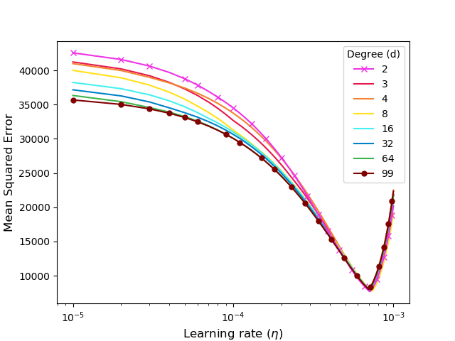
(a) Linear regression on CT dataset, M=100

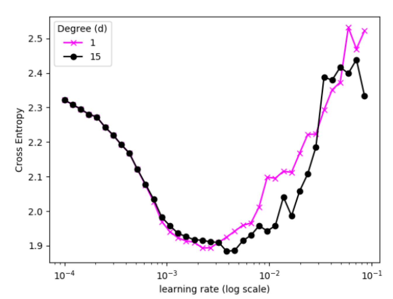
(b) ResNet18 on MNIST dataset, M=16

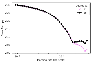
(c) 2-conv layers on MNIST, M=16

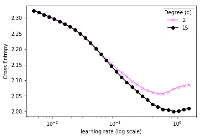
(d) ResNet18 on CIFAR-10, M=16

Figure 9: Error after one iteration vs learning rate.

In comparison to Table 1, Table 4 also shows the predictions for an “intermediate” bound, obtained by replacing in (8) $R$ with $R_{\textrm{sp}}{}$. These predictions are denoted by $k^{\prime\prime}_{o}$. Comparing $k^{\prime\prime}_{o}$ with $k^{\prime}_{o}$ and $k^{\prime}_{n}$ reveals that the difference between $k^{\prime}_{o}$ and $k^{\prime}_{n}$ is mainly due to the effect of $E_{\textrm{sp}}$, $H$, and $\alpha$, while $R_{\textrm{sp}}{}$ plays a less important role.

Table 4: Empirical estimation of $E$, $E_{\textrm{sp}}$, $H$, $\alpha$ on different ML problems and comparison of their joint effect ($\beta$) with the value $\widehat{\beta}$ predicted through (12). Number of iterations by which training losses for the ring and the clique differ by $4\%$, $10\%$, as predicted by the old bound (8), $k^{\prime}_{o}$, by the old bound (8) where $R$ is replaced by $R_{sp}$, $k^{{}^{\prime\prime}}_{o}$, by the new one (7), $k^{\prime}_{n}$, and as measured in the experiment, $k^{\prime}$. When their values exceeds the total number of iterations we ran (respectively 1200 for CT, 1190 for MNIST, and 1040 for CIFAR-10), we simply indicate it as $\infty$.

Dataset	Model	M	B	$\sqrt{E/E_{sp}}$	$\sqrt{E}/H$	$\frac{1}{\alpha}$	$\beta$	$\widehat{\beta}$	$@4\%$				$@10\%$
									$k^{\prime}_{o}$	$k^{{}^{\prime\prime}}_{o}$	$k^{\prime}_{n}$	$k^{\prime}$	$k^{\prime}_{o}$	$k^{{}^{\prime\prime}}_{o}$	$k^{\prime}_{n}$	$k^{\prime}$
CT (S=52000)	Linear regr. n=384	16	128	7.92	1.01	1.53	12.23	12.31	1	2	$\infty$	$\infty$	1	5	$\infty$	$\infty$
			3250	38.45	1.00	1.64	62.86	60.97	1	2	$\infty$	$\infty$	1	5	$\infty$	$\infty$
		100	128	7.75	1.01	1.54	12.05	11.56	1	2	10	$\infty$	1	4	$\infty$	$\infty$
			520	15.58	1.00	1.51	23.60	22.96	1	2	17	$\infty$	1	4	$\infty$	$\infty$
MNIST (S=60000)	2-conv layers n=431080	16	128	1.45	1.42	1.49	3.07	2.92	1	5	16	$\infty$	1	11	72	$\infty$
			500	2.15	1.14	1.53	3.75	3.71	1	6	22	40	1	14	260	$\infty$
		64	128	1.41	1.42	1.51	3.02	3.03	1	5	10	$\infty$	1	11	24	$\infty$
split by digit		10	500	1.01	1.00	1.42	1.42	3.62	1	2	3	60	1	3	7	100
CIFAR-10 (S= 50000)	ResNet18 n=11173962	16	128	1.07	3.35	1.49	5.34	5.62	1	2	10	30	1	4	20	$\infty$
			500	1.18	1.91	1.50	3.40	3.52	1	10	21	$\infty$	1	20	250	$\infty$

Figures 10(a) and 10(b) show the Cumulative Distribution Functions of computing times for the Spark cluster and for ASCI Q super-computer, respectively.

The following experiments have been carried out:

1. Linear regression on CT dataset on undirected expanders with computation time distribution from the Spark cluster (Fig. 11) and from ASCI Q super-computer (Fig. 12).

2. ResNet18 on MNIST dataset on directed ring lattices with computation time distribution from the Spark cluster (Fig. 13).

3. 2-conv layers on MNIST dataset on undirected expanders with computation time distribution from ASCI Q super-computer (Fig. 14)

4. ResNet18 on CIFAR-10 dataset on undirected expanders with computation time distribution from the Spark cluster (Fig. 15) and from ASCI Q super-computer (Fig. 16).

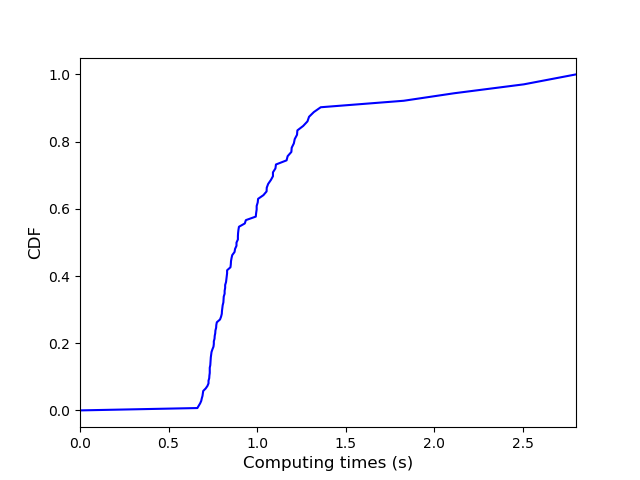
(a) Spark cluster

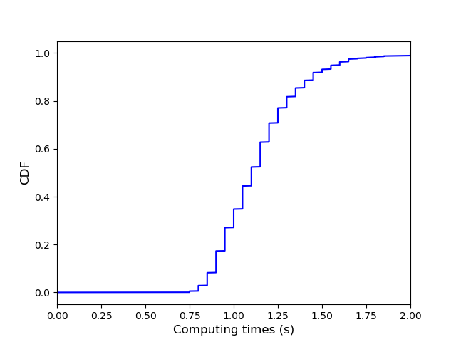
(b) ASCI Q

Figure 10: Empirical distribution of the computation times.

(a) Error vs iterations

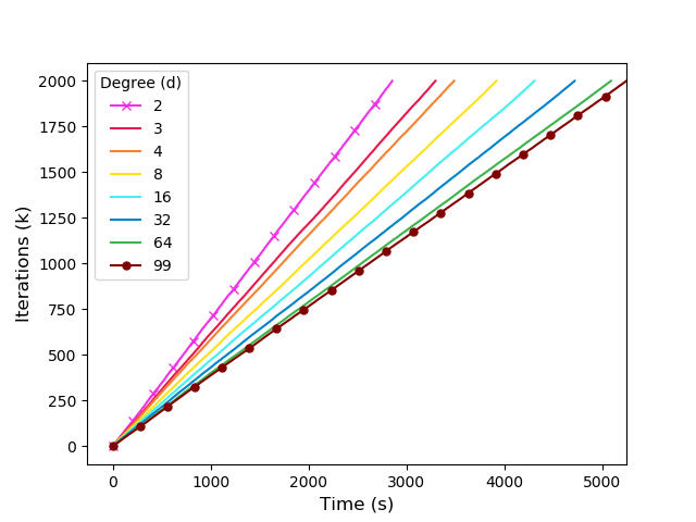
(b) Throughput

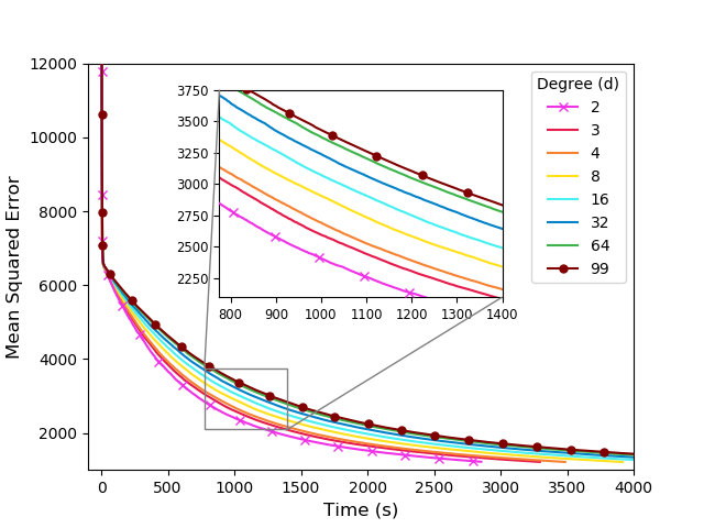
(c) Error vs time

Figure 11: Effect of network connectivity (degree $d$) on the convergence for linear regression on dataset CT with computation times from a Spark cluster. M = 100, B = 128.

(a) Error vs iterations

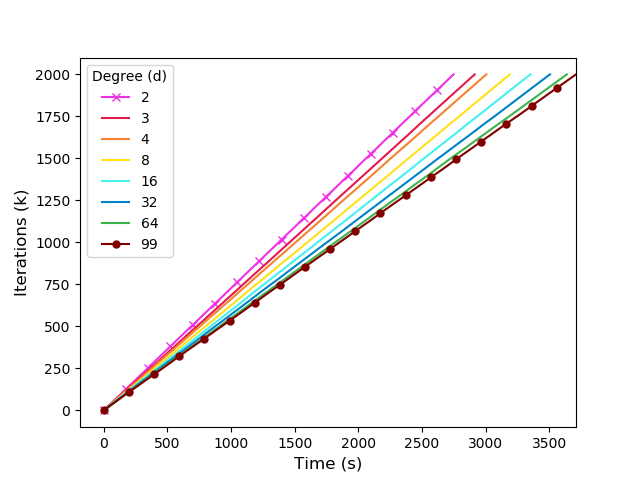
(b) Throughput

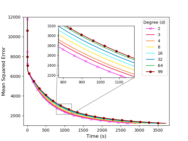
(c) Error vs time

Figure 12: Effect of network connectivity (degree $d$) on the convergence for linear regression on dataset CT with computation times from ASCI-Q super-computer. M = 100, B = 128.

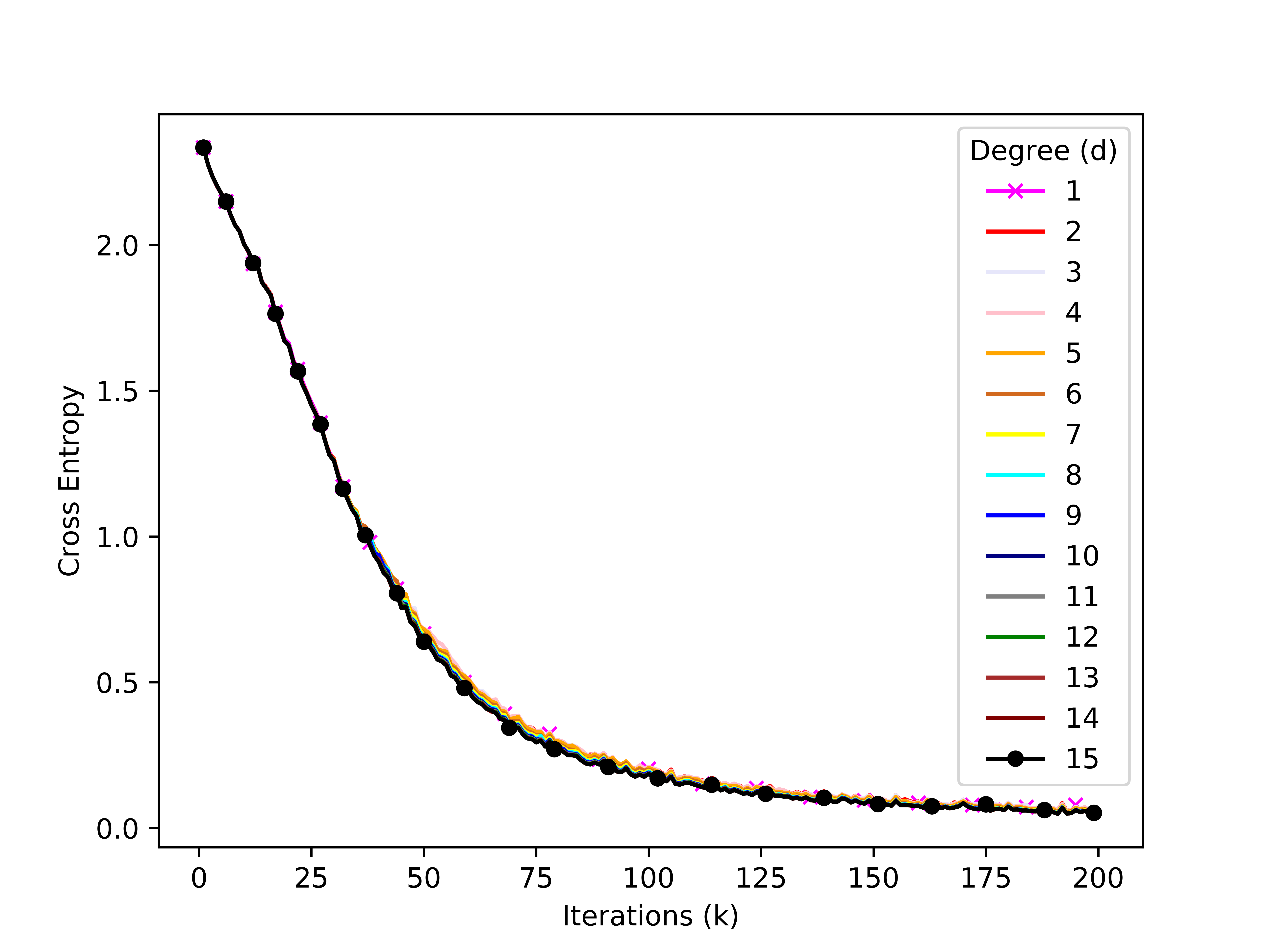
(a) Error vs iterations

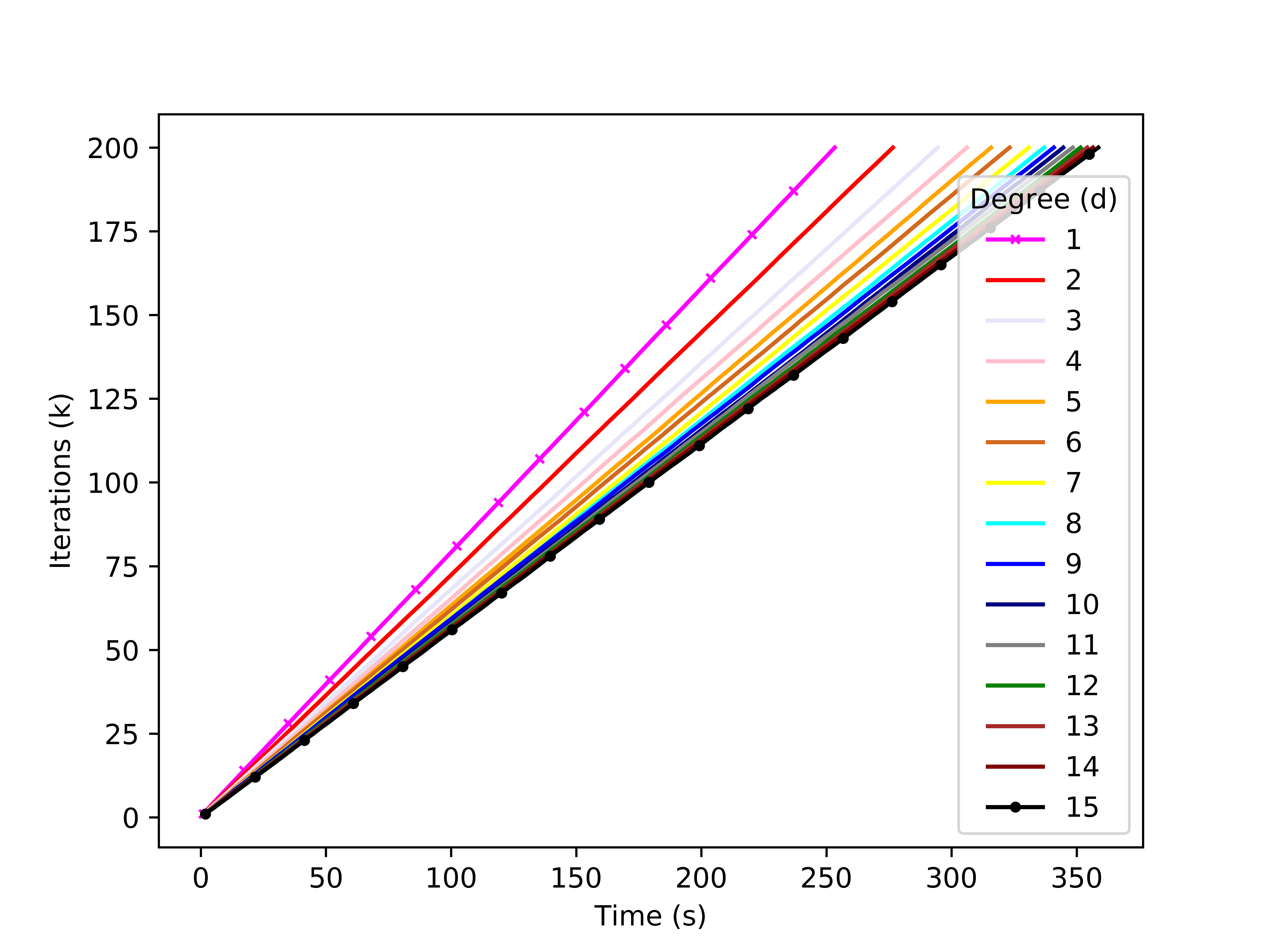
(b) Throughput

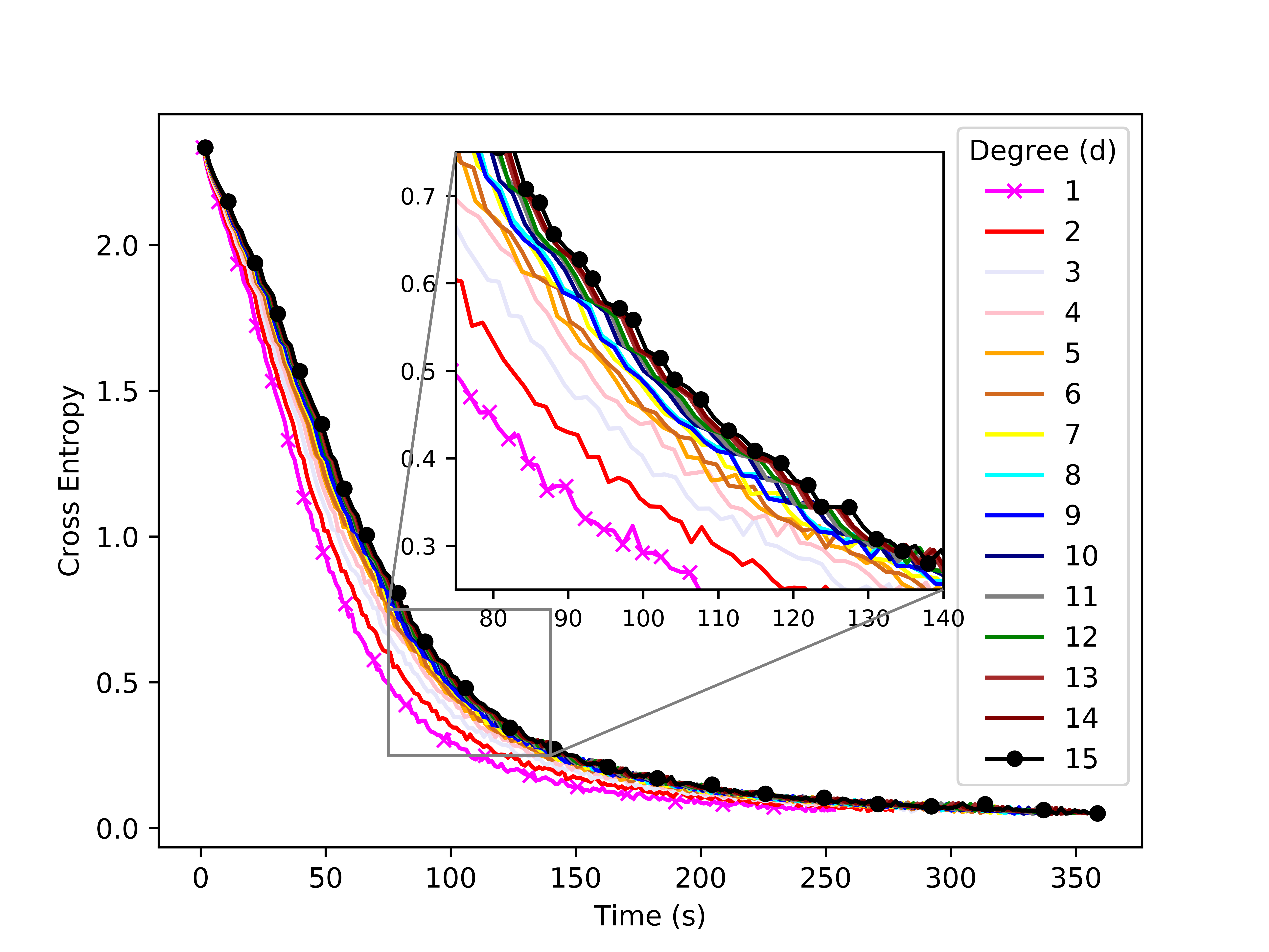
(c) Error vs time

Figure 13: Effect of network connectivity (degree $d$) on the convergence for ResNet18 on dataset MNIST with computation times from a Spark cluster. M = 16, B = 500.

(a) Error vs iterations

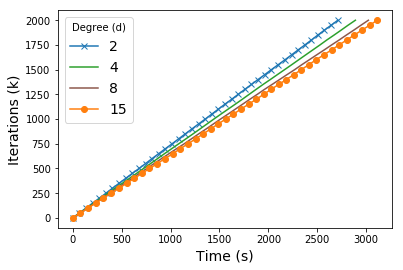
(b) Throughput

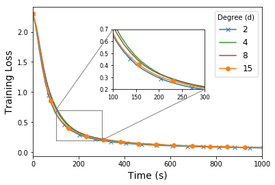
(c) Error vs time

Figure 14: Effect of network connectivity (in-degree $d$) on the convergence for 2-conv layers on dataset MNIST with computation times from ASCI-Q super-computer. M = 16, B = 500.

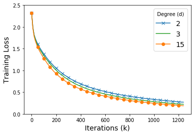
(a) Error vs iterations

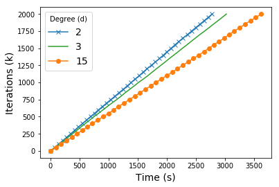
(b) Throughput

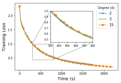
(c) Error vs time

Figure 15: Effect of network connectivity (degree $d$) on the convergence for CIFAR-10 with computation times from a spark cluster. M = 16, B = 128.

(a) Error vs iterations

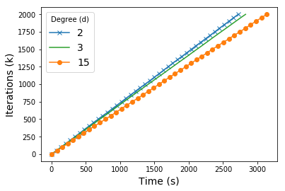
(b) Throughput

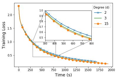
(c) Error vs time

Figure 16: Effect of network connectivity (degree $d$) on the convergence for CIFAR-10 with computation times from ASCI-Q super computer. M = 16, B = 128.

References

- (1) UCI Machine Learning Repository. http://archive.ics.uci.edu/ml/datasets/.
- Abadi et al. (2016) Martín Abadi, Paul Barham, Jianmin Chen, Zhifeng Chen, Andy Davis, Jeffrey Dean, Matthieu Devin, Sanjay Ghemawat, Geoffrey Irving, Michael Isard, Manjunath Kudlur, Josh Levenberg, Rajat Monga, Sherry Moore, Derek G. Murray, Benoit Steiner, Paul Tucker, Vijay Vasudevan, Pete Warden, Martin Wicke, Yuan Yu, and Xiaoqiang Zheng. Tensorflow: A system for large-scale machine learning. In Proceedings of the 12th USENIX Conference on Operating Systems Design and Implementation, OSDI’16, pages 265–283, 2016. ISBN 978-1-931971-33-1.
- Ananthanarayanan et al. (2013) Ganesh Ananthanarayanan, Ali Ghodsi, Scott Shenker, and Ion Stoica. Effective straggler mitigation: Attack of the clones. In Proc. of the 10th USENIX Conf. NSDI, 2013.
- Assran et al. (2019) Mahmoud Assran, Nicolas Loizou, Nicolas Ballas, and Michael Rabbat. Stochastic gradient push for distributed deep learning. In Proceedings of the 36th International Conference on Machine Learning, ICML 2019, volume 97 of Proceedings of Machine Learning Research, pages 344–353. PMLR, 2019.
- Baldi et al. (2014) Pierre Baldi, Peter Sadowski, and Daniel Whiteson. Searching for exotic particles in high-energy physics with deep learning. Nature communications, 5:4308, 2014.
- Canini et al. (2014) Kevin Canini, Tushar Chandra, Eugene Ie, Jim McFadden, Ken Goldman, Mike Gunter, Jeremiah Harmsen, Kristen LeFevre, Dmitry Lepikhin, Tomas Lloret Llinares, Indraneel Mukherjee, Fernando Pereira, Josh Redstone, Tal Shaked, and Yoram Singer. Sibyl: A system for large scale supervised machine learning, 2014. Technical talk.
- Duchi et al. (2012) John C. Duchi, Alekh Agarwal, and Martin J. Wainwright. Dual averaging for distributed optimization: Convergence analysis and network scaling. IEEE Trans. on Automatic Control, 57(3):592–606, 2012.
- Gibiansky (2017) Andrew Gibiansky. Bringing hpc techniques to deep learning. online, http://research.baidu.com/bringing-hpc-techniques-deep-learning, 2017.
- Google I/O (2018) Google I/O. Distributed tensorflow training. online, https://www.youtube.com/watch?v=bRMGoPqsn20, 2018.
- Graf et al. (2011) Franz Graf, Hans-Peter Kriegel, Matthias Schubert, Sebastian Pölsterl, and Alexander Cavallaro. 2D Image Registration in CT Images Using Radial Image Descriptors. In Proc. of MICCAI, pages 607–614, 2011.
- He et al. (2016) Kaiming He, Xiangyu Zhang, Shaoqing Ren, and Jian Sun. Deep residual learning for image recognition. In Proceedings of the IEEE conference on computer vision and pattern recognition, pages 770–778, 2016.
- Karakus et al. (2017) Can Karakus, Yifan Sun, Suhas Diggavi, and Wotao Yin. Straggler mitigation in distributed optimization through data encoding. In Proc. of NIPS, pages 5434–5442. 2017.
- Koloskova et al. (2019) Anastasia Koloskova, Sebastian U. Stich, and Martin Jaggi. Decentralized stochastic optimization and gossip algorithms with compressed communication. In Proceedings of the 36th International Conference on Machine Learning, ICML, volume 97 of Proceedings of Machine Learning Research, pages 3478–3487. PMLR, 2019.
- Konecný et al. (2015) Jakub Konecný, Brendan McMahan, and Daniel Ramage. Federated Optimization: Distributed Optimization Beyond the Datacenter. In Neural Information Processing Systems (workshop), 2015.
- Krizhevsky (2009) Alex Krizhevsky. Learning multiple layers of features from tiny images. Technical report, 2009.
- Lecun et al. (1998) Y. Lecun, L. Bottou, Y. Bengio, and P. Haffner. Gradient-based learning applied to document recognition. Proceedings of the IEEE, 86(11):2278–2324, Nov 1998.
- Li et al. (2014) Mu Li, David G Andersen, Alexander J Smola, and Kai Yu. Communication efficient distributed machine learning with the parameter server. In Z. Ghahramani, M. Welling, C. Cortes, N. D. Lawrence, and K. Q. Weinberger, editors, Advances in Neural Information Processing Systems 27, pages 19–27. Curran Associates, Inc., 2014.
- Li et al. (2018) Songze Li, Seyed Mohammadreza Mousavi Kalan, A. Salman Avestimehr, and Mahdi Soltanolkotabi. Near-Optimal Straggler Mitigation for Distributed Gradient Methods. In Proc. of the 7th Intl. Workshop ParLearning, May 2018.
- Lian et al. (2017) Xiangru Lian, Ce Zhang, Huan Zhang, Cho-Jui Hsieh, Wei Zhang, and Ji Liu. Can Decentralized Algorithms Outperform Centralized Algorithms? A Case Study for Decentralized Parallel Stochastic Gradient Descent. In NIPS, 2017.
- Lian et al. (2018) Xiangru Lian, Wei Zhang, Ce Zhang, and Ji Liu. Asynchronous decentralized parallel stochastic gradient descent. In ICML, 2018.
- Luo et al. (2019) Qinyi Luo, Jinkun Lin, Youwei Zhuo, and Xuehai Qian. Hop: Heterogeneity-aware decentralized training. In Proceedings of the Twenty-Fourth International Conference on Architectural Support for Programming Languages and Operating Systems, ASPLOS ’19, pages 893–907, 2019.
- McKay (1981) Brendan D. McKay. The expected eigenvalue distribution of a large regular graph. Linear Algebra and its Applications, 40:203 – 216, 1981.
- McKay and Wormald (1990) Brendan D. McKay and Nicholas C. Wormald. Uniform generation of random regular graphs of moderate degree. J. Algorithms, 11(1):52–67, February 1990. ISSN 0196-6774.
- Meyer (2000) Carl D. Meyer, editor. Matrix Analysis and Applied Linear Algebra. SIAM, Philadelphia, PA, USA, 2000. ISBN 0-89871-454-0.
- Nedić and Ozdaglar (2009) Angelia Nedić and Asuman E. Ozdaglar. Distributed subgradient methods for multi-agent optimization. IEEE Trans. Automat. Contr., 54(1):48–61, 2009.
- Nedić et al. (2018) Angelia Nedić, Alex Olshevsky, and Michael G. Rabbat. Network topology and communication-computation tradeoffs in decentralized optimization. Proc. of the IEEE, 106(5):953–976, May 2018.
- Neglia et al. (2019) Giovanni Neglia, Gianmarco Calbi, Don Towsley, and Gayane Vardoyan. The Role of Network Topology for Distributed Machine Learning. In IEEE International Conference on Computer Communications (INFOCOM), 2019.
- Pace et al. (2017) Francesco Pace, Daniele Venzano, Damiano Carra, and Pietro Michiardi. Flexible scheduling of distributed analytic applications. In Proceedings of the 17th IEEE/ACM International Symposium on Cluster, Cloud and Grid Computing, CCGrid ’17, pages 100–109, Piscataway, NJ, USA, 2017. IEEE Press. ISBN 978-1-5090-6610-0.
- Petrini et al. (2003) Fabrizio Petrini, Darren J. Kerbyson, and Scott Pakin. The case of the missing supercomputer performance: Achieving optimal performance on the 8,192 processors of asci q. In Proceedings of the 2003 ACM/IEEE Conference on Supercomputing, SC ’03, pages 55–, 2003.
- Pu et al. (2019) Shi Pu, Alex Olshevsky, and Ioannis Ch. Paschalidis. A non-asymptotic analysis of network independence for distributed stochastic gradient descent, 2019. arXiv preprint arXiv:1906.02702v9.
- Smith (2017) Leslie N Smith. Cyclical learning rates for training neural networks. In Applications of Computer Vision (WACV), 2017 IEEE Winter Conference on, pages 464–472. IEEE, 2017.
- Smola and Narayanamurthy (2010) Alexander Smola and Shravan Narayanamurthy. An architecture for parallel topic models. Proc. VLDB Endow., 3(1-2):703–710, September 2010. ISSN 2150-8097.
- Sutskever et al. (2013) Ilya Sutskever, James Martens, George Dahl, and Geoffrey Hinton. On the importance of initialization and momentum in deep learning. In International conference on machine learning, pages 1139–1147, 2013.
- Tsitsiklis et al. (1986) John Tsitsiklis, Dimitri Bertsekas, and Michael Athans. Distributed asynchronous deterministic and stochastic gradient optimization algorithms. IEEE Transactions on Automatic Control, 31(9):803–812, September 1986.
- Young et al. (2017) Steven R. Young, Derek C. Rose, Travis Johnston, William T. Heller, Thomas P. Karnowski, Thomas E. Potok, Robert M. Patton, Gabriel Perdue, and Jonathan Miller. Evolving Deep Networks Using HPC. In Proceedings of the Machine Learning on HPC Environments, MLHPC’17, 2017.