KeypointNet: A Large-scale 3D Keypoint Dataset
Aggregated from Numerous Human Annotations

Abstract

Detecting 3D objects keypoints is of great interest to the areas of both graphics and computer vision. There have been several 2D and 3D keypoint datasets aiming to address this problem in a data-driven way. These datasets, however, either lack scalability or bring ambiguity to the definition of keypoints. Therefore, we present KeypointNet: the first large-scale and diverse 3D keypoint dataset that contains 103,450 keypoints and 8,234 3D models from 16 object categories, by leveraging numerous human annotations. To handle the inconsistency between annotations from different people, we propose a novel method to aggregate these keypoints automatically, through minimization of a fidelity loss. Finally, ten state-of-the-art methods are benchmarked on our proposed dataset. Our code and data are available on https://github.com/qq456cvb/KeypointNet.

1 Introduction

Detection of 3D keypoints is essential in many applications such as object matching, object tracking, shape retrieval and registration [22, 6, 37]. Utilization of keypoints to match 3D objects has its advantage of providing features that are semantically significant and such keypoints are usually made invariant to rotations, scales and other transformations.

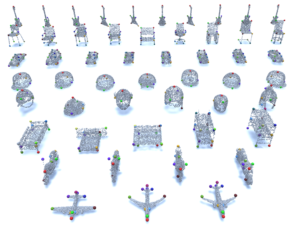
Figure 1: We propose a large-scale KeypointNet dataset. It contains 8K+ models and 103K+ keypoint annotations.

In the trend of deep learning, 2D semantic point detection has been boosted with the help of a large quantity of high-quality datasets [3, 23]. However, there are few 3D datasets focusing on the keypoint representation of an object. Dutagaci et al. [11] collect 43 models and label them according to annotations from various persons. Annotations from different persons are finally aggregated by geodesic clustering. ShapeNetCore keypoint dataset [42], and a similar dataset [15], in another way, resort to an expert’s annotation on keypoints, making them vulnerable and biased.

In order to alleviate the bias of experts’ definitions on keypoints, we ask a large group of people to annotate various keypoints according to their own understanding. Challenges rise in that different people may annotate different keypoints and we need to identify the consensus and patterns in these annotations. Finding such patterns is not trivial when a large set of keypoints spread across the entire model. A simple clustering would require a predefined distance threshold and fail to identify closely spaced keypoints. As shown in Figure 1, there are four closely spaced keypoints on each airplane empennage and it is extremely hard for simple clustering methods to distinguish them. Besides, clustering algorithms do not give semantic labels of keypoints since it is ambiguous to link clustered groups with each other. In addition, people’s annotations are not always exact and errors of annotated keypoint locations are inevitable. In order to solve these problems, we propose a novel method to aggregate a large number of keypoint annotations from distinct people, by optimizing a fidelity loss. After this auto aggregation process, we verify these generated keypoints based on some simple priors such as symmetry.

In this paper, we build the first large-scale and diverse dataset named KeypointNet which contains 8,234 models with 103,450 keypoints. These keypoints are of high fidelity and rich in structural or semantic meanings. Some examples are given in Figure 1. We hope this dataset could boost semantic understandings of common objects.

In addition, we propose two large-scale keypoint prediction tasks: keypoint saliency estimation and keypoint correspondence estimation. We benchmark ten state-of-the-art algorithms with mIoU, mAP and PCK metrics. Results show that the detection and identification of keypoints remain a challenging task.

Dataset	Domain	Correspondence	Template-free	Instances	Categories	Keypoints	Format
FAUST [4]	human	$\surd$	$\times$	100	1	689K	mesh
SyncSpecCNN [42]	chair	$\surd$	$\times$	6243	1	$\sim$60K	point cloud
Dutagaci et al. [11]	general	$\times$	$\surd$	43	16	$<$1K	mesh
Kim et al. [16]	general	$\surd$	$\times$	404	4	$\sim$3K	mesh
PASCAL 3D+ [40]	general	$\times$	$\times$	36292	12	150K+	RGB w. 3D model
Ours	general	$\surd$	$\surd$	8234	16	103K+	point cloud & mesh

Table 1: Comparison of 3d keypoint datasets. Correspondence indicates whether keypoints are indexed correspondingly. Template-free indicates whether it avoids hardcoded keypoint templates.

In summary, we make the following contributions:

• To the best of our knowledge, we provide the first large-scale dataset on 3D keypoints, both in number of categories and keypoints.

• We come up with a novel approach on aggregating people’s annotations on keypoints, even if their annotations are independent from each other.

• We experiment with ten state-of-the-art benchmarks on our dataset, including point cloud, graph, voxel and local geometry based keypoint detection methods.

2 Related Work

2.1 Detection of Keypoints

Detection of 3D keypoints has been a very important task for 3D object understanding which can be used in many applications, such as object pose estimation, reconstruction, matching, segmentation, etc. Researchers have proposed various methods to produce interest points on objects to help further objects processing. Traditional methods like 3D Harris [31], HKS [32], Salient Points [7], Mesh Saliency [18], Scale Dependent Corners [24], CGF [14], SHOT [35], etc, exploit local reference frames (LRF) to extract geometric features as local descriptors. However, these methods only consider the local geometric information without semantic knowledge, which forms a gap between detection algorithms and human understanding.

Recent deep learning methods like SyncSpecCNN [42], deep functional dictionaries [33] are proposed to detect keypoints. Unlike traditional ones, these methods do not handle rotations well. Though some recent methods like S2CNN [9] and PRIN [43] try to fix this, deep learning methods still rely on ground-truth keypoint labels annotated by human with expert verification.

2.2 Keypoint Datasets

Keypoint datasets have its origin in 2D images, where plenty of datasets on human skeletons and object interest points are proposed. For human skeletons, MPII human pose dataset [3], MSCOCO keypoint challenge [1] and PoseTrack [2] annotate millions of keypoints on humans. For more general objects, SPair-71k [23] contains 70,958 image pairs with diverse variations in viewpoint and scale, with a number of corresponding keypoints on each image pair. PUB [36] provides 15 part locations on 11,788 images from 200 bird categories and PASCAL [5] provides keypoint annotations for 20 object categories. HAKE [19] provides numerous annotations on human interactiveness keypoints. ADHA [25] annotates key adverbs in videos, which is a sequence of 2D images.

Keypoint datasets on 3D objects, include Dutagaci et al. [11], SyncSpecCNN [42] and Kim et al. [15]. Dutagaci et al. [11] aggregates multiple annotations from different people with an ad-hoc method while the dataset is extremely small. Though SyncSpecCNN [42], Pavlakos et al. [26] and Kim et al. [15] give a relatively large keypoint dataset, they rely on a manually designed template of keypoints, which is inevitably biased and flawed. GraspNet [12] gives dense annotations on 3D object grasping. The differences between theirs and ours are illustrated in Table 1.

3 KeypointNet: A Large-scale 3D Keypoint Dataset

3.1 Data Collection

KeypointNet is built on ShapeNetCore [8]. ShapeNetCore covers 55 common object categories with about 51,300 unique 3D models.

We filter out those models that deviate from the majority and keep at most 1000 instances for each category in order to provide a balanced dataset. In addition, a consistent canonical orientation is established (e.g., upright and front) for every category because of the incomplete alignment in ShapeNetCore.

We let annotators determine which points are important, and same keypoint indices should indicate same meanings for each annotator. Though annotators are free to give their own keypoints, three general principles should be obeyed: (1) each keypoint should describe an object’s semantic information shared across instances of the same object category, (2) keypoints of an object category should spread over the whole object and (3) different keypoints have distinct semantic meanings. After that, we utilize a heuristic method to aggregate these points, which will be discussed in Section 4.

Keypoints are annotated on meshes and these annotated meshes are then downsampled to 2,048 points. Our final dataset is a collection of point clouds, with keypoint indices.

3.2 Annotation Tools

We develop an easy-to-use web annotation tool based on NodeJS. Every user is allowed to click up to 24 interest points according to his/her own understanding. The UI interface is shown in Figure 2. Annotated models are shown in the left panel while the next unprocessed model is shown in the right panel.

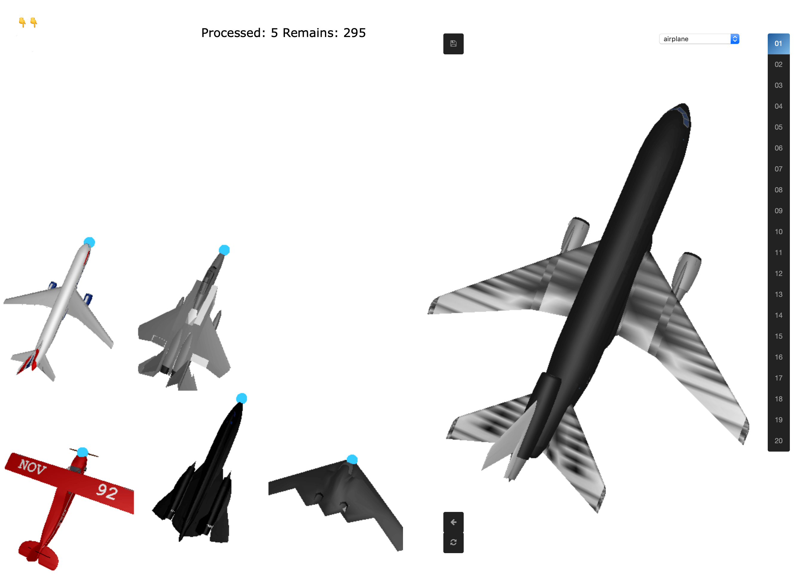
Figure 2: Web interface of the annotation tool.

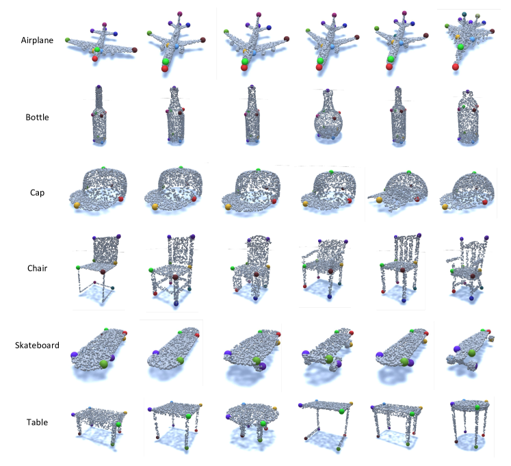
Figure 3: Dataset Visualization. Here we plot ground-truth keypoints for several categories. We can see that by utilizing our automatic aggregation method, keypoints of high fidelity are extracted.

3.3 Dataset Statistics

At the time of this work, our dataset has collected 16 common categories from ShapeNetCore, with 8234 models. Each model contains 3 to 24 keypoints. Our dataset is divided into train, validation and test splits, with 7:1:2 ratio. Table 3.3 gives detailed statistics of our dataset. Some visualizations of our dataset is given in Figure 3.

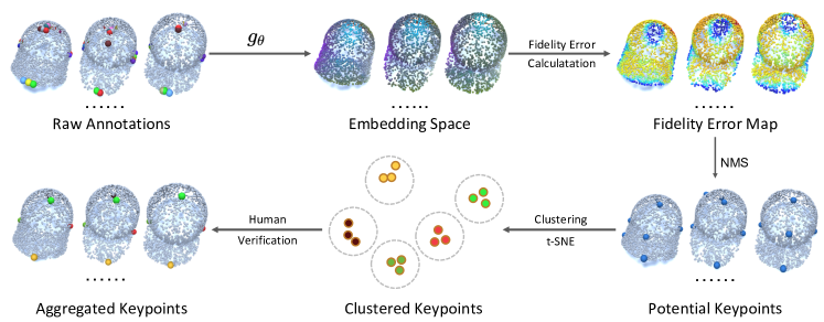
Figure 4: Keypoint aggregation pipeline. We first infer dense embeddings from human labeled raw annotations. Then fidelity error maps are calculated by summing embedding distances to human labeled keypoints. Non Minimum Suppression is conducted to form a potential set of keypoints. These keypoints are then projected onto 2D subspace with t-SNE and verified by humans.

tabularl—c—c—c—c—c @Category @Train @Val @Test @All @#Annotators
@Airplane 715 102 205 sum(b2:d2) 26
@Bathtub 344 49 99 sum(b3:d3) 15
@Bed 102 14 30 sum(b4:d4) 8
@Bottle 266 38 76 sum(b5:d5) 9
@Cap 26 4 8 sum(b6:d6) 6
@Car 701 100 201 sum(b7:d7) 17
@Chair 699 100 200 sum(b8:d8) 15
@Guitar 487 70 140 sum(b9:d9) 13
@Helmet 62 10 18 sum(b10:d10) 8
@Knife 189 27 54 sum(b11:d11) 5
@Laptop 307 44 88 sum(b12:d12) 12
@Motorcycle 208 30 60 sum(b13:d13) 7
@Mug 130 18 38 sum(b14:d14) 9
@Skateboard 98 14 29 sum(b15:d15) 9
@Table 786 113 225 sum(b16:d16) 17
@Vessel 637 91 182 sum(b17:d17) 18
@Total sum(b2:b17) sum(c2:c17) sum(d2:d17) sum(e2:e17) sum(f2:f17)

tabularl—c—c—c—c @Category @Train @Val @Test @All
@Airplane 9695 1379 2756 sum(b2:d2)
@Bathtub 5519 772 1589 sum(b3:d3)
@Bed 1276 188 377 sum(b4:d4)
@Bottle 4366 625 1269 sum(b5:d5)
@Cap 154 24 48 sum(b6:d6)
@Car 14976 2133 4294 sum(b7:d7)
@Chair 8488 1180 2395 sum(b8:d8)
@Guitar 4112 591 1197 sum(b9:d9)
@Helmet 529 85 162 sum(b10:d10)
@Knife 946 136 276 sum(b11:d11)
@Laptop 1842 264 528 sum(b12:d12)
@Motorcycle 2690 394 794 sum(b13:d13)
@Mug 1427 198 418 sum(b14:d14)
@Skateboard 903 137 283 sum(b15:d15)
@Table 6325 913 1809 sum(b16:d16)
@Vessel 9168 1241 2579 sum(b17:d17)
@Total sum(b2:b17) sum(c2:c17) sum(d2:d17) sum(e2:e17)

Table 2: Keypoint Dataset statistics. Left: number of models in each category. Right: number of keypoints in each category.

4 Keypoint Aggregation

Given all human labeled raw keypoints, we leverage a novel method to aggregate them together into a set of ground-truth keypoints.

There are generally two reasons: 1) distinct people may annotate different sets of keypoints and human labeled keypoints are sometimes erroneous, so we need an elegant way to aggregate these keypoints; 2) a simple clustering algorithm would fail to distinguish those closely spaced keypoints and cannot give consistent semantic labels.

4.1 Problem Statement

Given a $2$-dimensional sub-manifold $\mathcal{M}_{m}\subset\mathbb{R}^{3}$, where $m$ is the index of the model, a valid annotation from the $c$-th person is a keypoint set $\{l_{m,k}^{(c)}|l_{m,k}^{(c)}\in\mathcal{M}_{m}\}_{k=1}^{K_{c}}$, where $k$ is the keypoint index and $K_{c}$ is the number of keypoints annotated by person $c$. Note that different people may have different sets of keypoint indices and these indices are independent.

Our goal is to aggregate a set of potential ground-truth keypoints $\mathcal{Y}=\{y_{m,k}|y_{m,k}\in\mathcal{M}_{m},m=1,\dots M,k=1,\dots K_{m}\}$, where ${K_{m}}$ is the number of proposed keypoints for each model $\mathcal{M}_{m}$, so that $y_{m_{1},k}$ and $y_{m_{2},k}$ share the same semantic.

4.2 Keypoint Saliency

Each annotation is allowed to be erroneous within a small region, so that a keypoint distribution is defined as follows:

$$p(x|x\text{ is the $k$-th keypoint},x\in\mathcal{M}_{m})=\frac{\phi(l_{m,k},x)}{Z(\phi)},$$

where $\phi$ is Gaussian kernel function. $Z$ is a normalization constant. This contradicts many previous methods on annotating keypoints where a $\delta$-function is implicitly assumed. We argue that it is common that humans make mistakes when annotating keypoints and due to central limit theorem, the keypoint distribution would form a Gaussian.

4.3 Ground-truth Keypoint Generation

We propose to jointly output a dense mapping function $g_{\theta}:\mathcal{M}\rightarrow\mathbb{R}^{d}$ whose parameters are $\theta$, and the aggregated ground-truth keypoint set $\mathcal{Y}$. $g_{\theta}$ transforms each point into an high-dimensional embedding vector in $\mathbb{R}^{d}$. Specifically, we solve the following optimization problem:

$$\begin{split}(\theta^{\ast},\mathcal{Y}^{\ast})&=\operatorname*{arg\,min}_{\theta,\mathcal{Y}}[f(\mathcal{Y},g_{\theta})+H(g_{\theta})]\\ &s.t.\ g_{\theta}(y_{m_{1},k})\equiv g_{\theta}(y_{m_{2},k}),\forall m_{1},m_{2},k.\end{split}$$ (1)

where $f(\mathcal{Y},g_{\theta})$ is the data fidelity loss and $H(g_{\theta})$ is a regularization term to avoid trivial solution like $g_{\theta}\equiv 0$. The constraint states that the embedding of ground-truth keypoints with the same index should be the same.

Fidelity Loss

We define $f(\mathcal{Y},g_{\theta})$ as:

$$f(\mathcal{Y},g_{\theta})=\sum_{m=1}^{M}\sum_{c=1}^{C}\sum_{k=1}^{K_{m}}\int_{\mathcal{M}_{m}}\mathbf{d}_{\theta}(x,y_{m,k})\frac{\phi(l_{m,n^{*}}^{(c)},x)}{Z(\phi)}dx,$$

where $\mathbf{d}_{\theta}$ is the L2 distance between two vectors in embedding space:

$$\mathbf{d}_{\theta}(a,b)=\|g_{\theta}(a)-g_{\theta}(b)\|_{2}^{2},$$

and

$$n^{*}=\operatorname*{arg\,min}_{n}\mathbf{d}_{\theta}({l_{m,n}^{(c)}},y_{m}).$$

Unlike previous methods such as Dutagaci et al.[11] where a simple geodesic average of human labeled points is given as ground-truth points, we seek a point whose expected embedding distance to all human labeled points is smallest. The reason is that geodesic distance is sensitive to the misannotated keypoints and could not distinguish closely spaced keypoints, while embedding distance is more robust to noisy points as the embedding space encodes the semantic information of an object.

Equation 1 involves both $\theta$ and $\mathcal{Y}$ and it is impractical to solve this problem in closed form. In practice, we use alternating minimization with a deep neural network to approximate the embedding function $g_{\theta}$, so that we solve the following dual problem instead (by slightly loosening the constraints):

$$\begin{split}\theta^{\ast}=&\operatorname*{arg\,min}_{\theta}[H(g_{\theta})\\ &+\lambda\sum_{m_{1},m_{2}}^{M}\sum_{k}^{K_{m}}\|g_{\theta}(y_{m_{1},k})-g_{\theta}(y_{m_{2},k})\|_{2}^{2}],\end{split}$$ (2)

$$\begin{split}\mathcal{Y}^{\ast}=\operatorname*{arg\,min}_{\mathcal{Y}}&\sum_{m=1}^{M}\sum_{c=1}^{C}\sum_{k=1}^{K_{m}}\int_{\mathcal{M}_{m}}\mathbf{d}_{\theta}(x,y_{m,k})\frac{\phi(l_{m,n^{\star}}^{(c)},x)}{Z(\phi)}dx,\\ &s.t.\ g_{\theta}(y_{m_{1},k})\equiv g_{\theta}(y_{m_{2},k}),\forall m_{1},m_{2},k,\end{split}$$ (3)

and alternate between the two equations until convergence.

By solving this problem, we find both an optimal embedding function $g_{\theta}$, together with intra-class consistent ground-truth keypoints $\mathcal{Y}$, while keeping its embedding distance from human-labeled keypoints as close as possible. The ground-truth keypoints can be viewed as the projection of human labeled data onto embedding space.

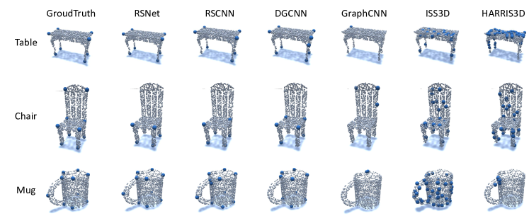
Figure 5: Visualizations of detected keypoints for six algorithms.

	Airplane	Bathtub	Bed	Bottle	Cap	Car	Chair	Guitar	Helmet	Knife	Laptop	Motor	Mug	Skate	Table	Vessel	Average
PointNet	10.4/9.3	0.8/6.3	3.0/9.4	0.5/8.2	0.0/0.3	7.3/9.2	7.7/6.5	0.1/1.4	0.0/1.3	0.0/0.9	23.6/32.0	0.1/4.0	0.2/3.9	0.0/2.9	20.9/23.1	7.1/9.1	5.1/8.0
PointNet++	33.5/44.6	18.5/32.3	16.4/23.4	22.1/38.2	13.2/12.1	24.0/41.0	18.2/29.4	24.3/27.7	7.0/7.4	19.0/22.1	30.9/60.0	21.9/36.0	16.3/21.4	13.7/16.1	29.3/47.4	16.7/26.9	20.3/30.4
RSNet	33.7/38.8	23.1/36.0	28.4/42.5	29.4/44.3	26.7/26.9	30.4/42.3	22.7/26.2	30.5/34.2	15.8/21.3	21.7/31.5	39.8/62.0	31.5/43.2	24.1/35.2	21.6/25.9	39.7/54.6	18.3/22.3	27.3/36.7
SpiderCNN	24.6/24.7	13.0/16.4	16.4/17.1	3.6/8.2	0.0/0.5	11.8/17.2	18.2/20.4	7.4/9.9	0.0/0.5	14.9/18.7	25.6/40.0	12.0/13.3	2.2/4.0	1.8/3.3	27.9/40.5	12.9/14.6	12.0/15.6
PointConv	40.0/51.2	29.0/44.7	25.1/43.7	33.6/46.5	0.0/7.0	35.9/55.6	25.5/39.8	28.0/39.3	7.7/8.3	26.6/38.1	43.1/63.5	35.9/50.6	19.8/32.0	9.3/10.1	44.1/64.0	21.7/31.8	26.6/39.1
RSCNN	31.1/45.0	20.4/34.9	26.2/40.1	25.6/40.1	7.0/8.9	25.4/44.7	22.0/33.0	27.3/34.1	8.9/10.8	21.1/27.2	35.2/58.8	23.6/37.0	15.9/18.6	21.9/30.1	27.4/49.8	18.1/28.9	22.3/33.9
DGCNN	39.2/52.0	25.5/40.6	32.4/42.8	40.3/61.6	0.0/2.0	27.0/48.6	24.9/34.6	31.9/44.1	17.1/19.9	31.5/39.9	44.8/69.6	30.3/41.4	23.9/33.2	22.6/29.8	41.0/59.0	24.4/35.6	28.5/40.9
GraphCNN	0.7/0.7	17.0/23.7	22.2/31.5	23.3/42.6	0.0/4.1	23.0/36.5	0.6/0.6	17.0/21.6	9.7/12.5	18.7/23.3	33.3/49.7	0.6/0.7	0.5/0.6	11.7/12.8	24.5/34.7	15.1/19.3	13.6/19.7
Harris3D	1.6/-	0.3/-	0.9/-	0.5/-	0.0/-	0.9/-	0.7/-	1.2/-	0.0/-	1.9/-	0.3/-	0.7/-	0.0/-	1.0/-	0.4/-	1.2/-	0.7/-
SIFT3D	1.2/-	1.0/-	0.5/-	1.1/-	0.4/-	1.0/-	0.7/-	0.7/-	0.4/-	0.6/-	0.2/-	0.8/-	0.5/-	0.7/-	0.3/-	1.0/-	0.7/-
ISS3D	1.1/-	1.4/-	0.9/-	1.8/-	0.6/-	1.7/-	0.7/-	0.7/-	0.8/-	0.4/-	0.1/-	0.8/-	0.9/-	0.8/-	0.3/-	1.1/-	0.9/-

Table 3: mIoU and mAP results (in percentage) for compared methods with distance threshold 0.01.

Non Minimum Suppression

Equation 3 may be hard to solve since $K_{m}$ is also unknown beforehand. For each model $\mathcal{M}_{m}$, the fidelity error associated with each potential keypoint $y_{m}\in\mathcal{M}_{m}$ is:

$$f(y_{m},g_{\theta})=\sum_{m^{\prime}\neq m}^{M}\sum_{c=1}^{C}\int_{\mathcal{M}_{m^{\prime}}}\mathbf{d}_{\theta}(x,y_{m^{\prime}})\frac{\phi(l_{{m^{\prime}},n^{*}}^{(c)},x)}{Z(\phi)}dx,$$ (4)

where $y_{m^{\prime}}=\operatorname*{arg\,min}_{y_{m^{\prime}}\in\mathcal{M}_{m^{\prime}}}\|g_{\theta}(y_{m^{\prime}})-g_{\theta}(y_{m})\|_{2}^{2}$.

Then $y_{m}^{\ast}$ is found by conducting Non Minimum Suppression (NMS), such that:

$$\begin{split}f(y_{m}^{\ast},g_{\theta})\leq f(y_{m},g_{\theta}),\\ \forall y_{m}\in\mathcal{M}_{m},\mathbf{d}_{\theta}(y_{m},y_{m}^{*})<\delta,\end{split}$$ (5)

where $\delta$ is some neighborhood threshold.

After NMS, we would get several ground-truth points $y_{m,1},y_{m,2},\dots,y_{m,k}$ for each manifold $\mathcal{M}_{m}$. However, the arbitrarily assigned index $k$ within each model does not provide a consistent semantic correspondence across different models. Therefore we cluster these points according to their embeddings by first projecting them onto 2D subspace with t-SNE [21].

Ground-truth Verification

Though the above method automatically aggregate a set of potential set of keypoints with high precision, it omits some keypoints in some cases. As the last step, experts manually verify these keypoints based on some simple priors such as the rotational symmetry and centrosymmetry of an object.

4.4 Implementation Details

At the start of the alternating minimization, we initialize $\mathcal{Y}$ to be sampled from raw annotations and then run one iteration, which is enough for the convergence. We choose PointConv with hidden dimension 128 as the embedding function $g$. During the optimization of Equation 3, we classify each point into $K$ classes with a SoftMax layer and extract the feature of the last but one layer as the embedding. The learning rate is 1e-3 and the optimizer is Adam [17].

4.5 Pipeline

The whole pipeline is shown in Figure 4. We first infer dense embeddings from human labeled raw annotations. Then fidelity error maps are calculated by summing embedding distances to human labeled keypoints. Non Minimum Suppression is conducted to form a potential set of keypoints. These keypoints are then projected onto 2D subspace with t-SNE and verified by humans.

5 Tasks and Benchmarks

In this section, we propose two keypoint prediction tasks: keypoint saliency estimation and keypoint correspondence estimation. Keypoint saliency estimation requires evaluated methods to give a set of potential indistinguishable keypoints while keypoint correspondence estimation asks to localize a fixed number of distinguishable keypoints.

5.1 Keypoint Saliency Estimation

Dataset Preparation

For keypoint saliency estimation, we only consider whether a point is the keypoint or not, without giving its semantic label. Our dataset is split into train, validation and test sets with the ratio 70%, 10%, 20%.

Evaluation Metrics

Two metrics are adopted to evaluate the performance of keypoint saliency estimation. Firstly, we evaluate their mean Intersection over Unions [34] (mIoU), which can be calculated as

$$\begin{split}IoU=\frac{TP}{TP+FP+FN}.\end{split}$$ (6)

mIoU is calculated under different error tolerances from 0 to 0.1. Secondly, for those methods that output keypoint probabilities, we evaluate their mean Average Precisions (mAP) over all categories.

Benchmark Algorithms

We benchmark eight state-of-the-art algorithms on point cloud semantic analysis: PointNet [27], PointNet++ [28], RSNet [13], SpiderCNN [41], PointConv [39], RSCNN [20], DGCNN [38] and GraphCNN [10]. Three traditional local geometric keypoint detectors are also considered: Harris3D [31], SIFT3D [29] and ISS3D [30].

Evaluation Results

For deep learning methods, we use the default network architectures and hyperparameters to predict the keypoint probability of each point and mIoU and mAP are adopted to evaluate their performance. For local geometry based methods, mIoU is used. Each method is tested with various geodesic error thresholds. In Table 3, we report mIoU and mAP results under a restrictive threshold 0.01. Figure  6 shows the mIoU curves under different distance thresholds from 0 to 0.1 and Figure 7 shows the mAP results. We can see that under a restrictive distance threshold 0.01, geometric and deep learning methods both fail to predict qualified keypoints.

Figure 5 shows some visualizations of the results from RSNet, RSCNN, DGCNN, GraphCNN, ISS3D and Harris3D. Deep learning methods can predict some of ground-truth keypoints while the predicted keypoints are sometimes missing. For local geometry based methods like ISS3D and Harris3D, they give much more interest points spread over the entire model while these points are agnostic of semantic information. Learning discriminative features for better localizing accurate and distinct keypoints across various objects is still a challenging task.

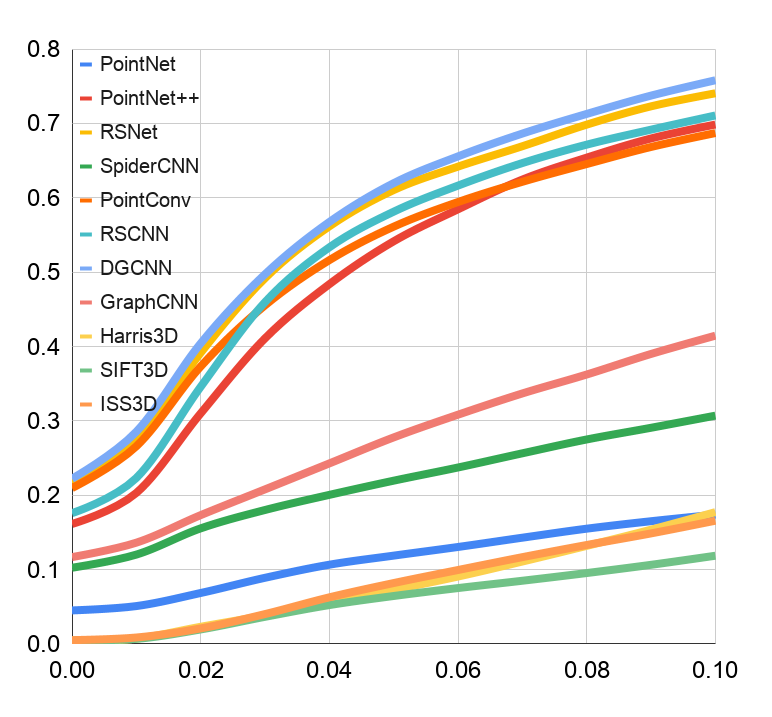
Figure 6: mIoU results under various distance thresholds (0-0.1) for compared algorithms.

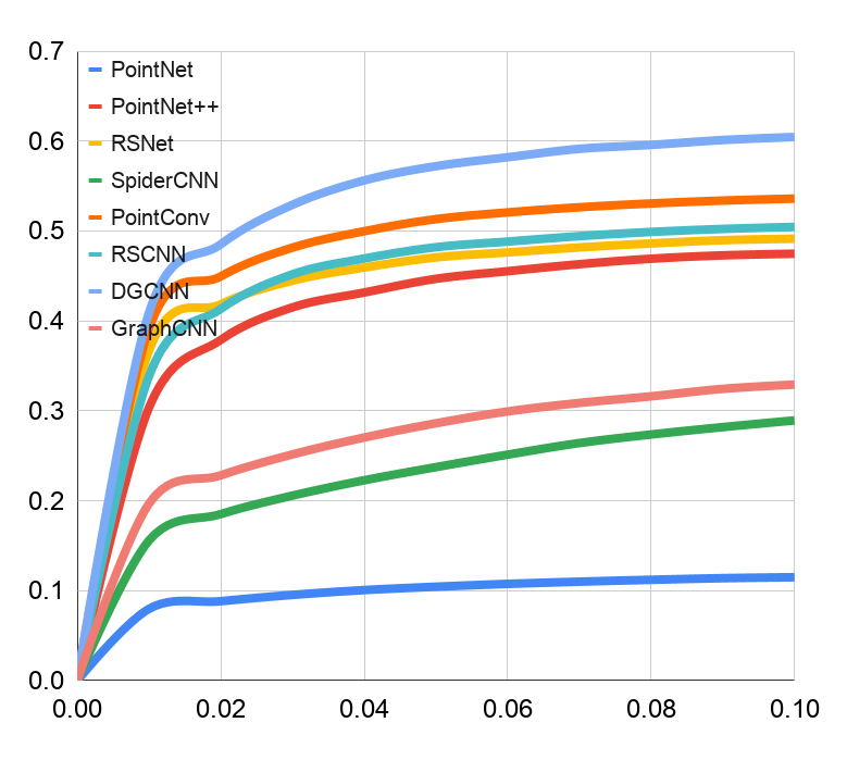
Figure 7: mAP results under various distance thresholds (0-0.1) for compared algorithms.

5.2 Keypoint Correspondence Estimation

Keypoint correspondence estimation is a more challenging task, where one needs to predict not only the keypoints, but also their semantic labels. The semantic labels should be consistent across different objects in the same category.

Dataset Preparation

For keypoint correspondence estimation, each keypoint is labeled with a semantic index. For those keypoints that do not exist on some objects, index -1 is given. Similar to SyncSpecCNN [42], the maximum number of keypoints is fixed and the data split is the same as keypoint saliency estimation.

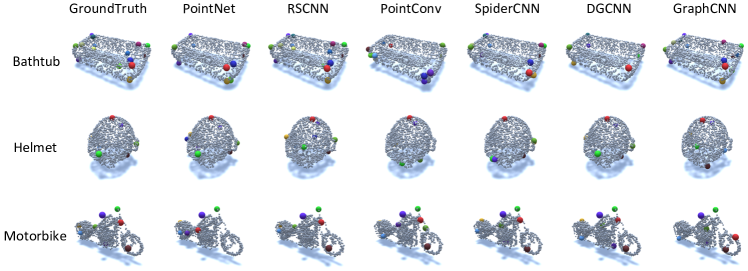
Figure 8: Visualizations of detected keypoints and their semantic labels. Same colors indicate same semantic labels.

	Airplane	Bath	Bed	Bottle	Cap	Car	Chair	Guitar	Helmet	Knife	Laptop	Motor	Mug	Skate	Table	Vessel	Average
PointNet	65.4	57.2	55.4	78.9	16.7	66.6	43.2	65.4	42.6	32.6	76.1	62.1	60.7	50.4	63.8	42.5	55.0
PointNet++	64.1	45.4	44.2	10.2	18.8	55.1	38.0	55.4	23.6	43.8	64.6	49.9	36.4	42.3	57.1	37.9	42.9
RSNet	68.9	56.0	69.2	78.2	47.9	65.7	49.4	63.7	33.8	56.9	80.3	67.4	61.7	69.2	72.3	46.7	61.7
SpiderCNN	54.9	36.8	43.9	50.4	0.0	47.1	36.9	37.7	5.6	32.2	63.4	36.6	16.4	15.8	61.0	36.8	36.0
PointConv	70.3	54.4	58.6	64.6	25.0	65.7	51.1	62.6	16.2	47.4	74.2	61.7	51.2	51.8	69.5	46.7	54.4
RSCNN	66.8	47.9	52.4	59.4	18.8	56.5	45.0	60.0	21.3	51.4	66.9	52.8	29.5	51.7	64.8	41.2	49.2
DGCNN	66.8	51.5	56.3	8.9	39.6	58.6	46.0	62.4	36.1	52.1	73.9	57.7	51.4	52.3	70.5	46.8	51.9
GraphCNN	41.8	19.5	35.4	32.1	8.3	36.9	27.0	28.9	8.8	20.0	65.9	34.4	15.6	26.2	17.3	22.1	27.5

Table 4: PCK results under distance threshold 0.01 for various deep learning networks.

Evaluation Metric

The prediction of network is evaluated by the percentage of correct keypoints (PCK), which is used to evaluate the accuracy of keypoint prediction in many previous works [42, 33].

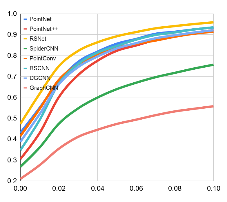
Figure 9: PCK results under various distance thresholds (0-0.1) for compared algorithms.

Benchmark Algorithms

We benchmark eight state-of-the-art algorithms: PointNet [27], PointNet++[28], RSNet [13], SpiderCNN [41], PointConv [39], RSCNN [20], DGCNN [38] and GraphCNN [10].

Evaluation Results

Similarly, we use the default network architectures. Table 4 shows the PCK results with error distance threshold 0.01. Figure 9 illustrates the percentage of correct points curves with distance thresholds varied from 0 to 0.1. RS-Net performs relatively better than the other methods under all thresholds. However, all eight methods face difficulty in giving exact consistent semantic keypoints under a threshold of 0.01.

Figure 8 shows some visualizations of the results for different methods. Same colors denote same semantic labels. We can see that most methods can accurately predict some of keypoints. However, there are still some missing keypoints and inaccurate localizations.

Keypoint saliency estimation and keypoint correspondence estimation are both important for object understanding. Keypoint saliency estimation gives a spare representation of object by extracting meaningful points. Keypoint correspondence estimation establishes relations between points on different objects. From the results above, we can see that these two tasks still remain challenging. The reason is that object keypoints from human perspective are not simply geometrically salient points but abstracts semantic meanings of the object.

6 Conclusion

In this paper, we propose a large-scale and high-quality KeypointNet dataset. In order to generate ground-truth keypoints from raw human annotations where identification of their modes are non-trivial, we transform the problem into an optimization problem and solve it in an alternating fashion. By optimizing a fidelity loss, ground-truth keypoints, together with their correspondences are generated. In addition, we evaluate and compare several state-of-the-art methods on our proposed dataset and we hope this dataset could boost the semantic understanding of 3D objects.

Acknowledgements

This work is supported in part by the National Key R&D Program of China (No. 2017YFA0700800), National Natural Science Foundation of China under Grants 61772332, 51675342, 51975350, SHEITC (2018-RGZN-02046) and Shanghai Science and Technology Committee.

References

- [1] Mscoco keypoint challenge 2016, 2016.
- [2] Mykhaylo Andriluka, Umar Iqbal, Eldar Insafutdinov, Leonid Pishchulin, Anton Milan, Juergen Gall, and Bernt Schiele. Posetrack: A benchmark for human pose estimation and tracking. In Proceedings of the IEEE Conference on Computer Vision and Pattern Recognition, pages 5167–5176, 2018.
- [3] Mykhaylo Andriluka, Leonid Pishchulin, Peter Gehler, and Bernt Schiele. 2d human pose estimation: New benchmark and state of the art analysis. In IEEE Conference on Computer Vision and Pattern Recognition (CVPR), June 2014.
- [4] Federica Bogo, Javier Romero, Matthew Loper, and Michael J. Black. FAUST: Dataset and evaluation for 3D mesh registration. In Proceedings IEEE Conf. on Computer Vision and Pattern Recognition (CVPR), Piscataway, NJ, USA, June 2014. IEEE.
- [5] Lubomir Bourdev and Jitendra Malik. Poselets: Body part detectors trained using 3d human pose annotations. In 2009 IEEE 12th International Conference on Computer Vision, pages 1365–1372. IEEE, 2009.
- [6] M Bueno, J Martínez-Sánchez, H González-Jorge, and H Lorenzo. Detection of geometric keypoints and its application to point cloud coarse registration. International Archives of the Photogrammetry, Remote Sensing & Spatial Information Sciences, 41, 2016.
- [7] Umberto Castellani, Marco Cristani, Simone Fantoni, and Vittorio Murino. Sparse points matching by combining 3d mesh saliency with statistical descriptors. In Computer Graphics Forum, volume 27, pages 643–652. Wiley Online Library, 2008.
- [8] Angel X Chang, Thomas Funkhouser, Leonidas Guibas, Pat Hanrahan, Qixing Huang, Zimo Li, Silvio Savarese, Manolis Savva, Shuran Song, Hao Su, et al. Shapenet: An information-rich 3d model repository. arXiv preprint arXiv:1512.03012, 2015.
- [9] Taco S Cohen, Mario Geiger, Jonas Köhler, and Max Welling. Spherical cnns. arXiv preprint arXiv:1801.10130, 2018.
- [10] Michaël Defferrard, Xavier Bresson, and Pierre Vandergheynst. Convolutional neural networks on graphs with fast localized spectral filtering. In Advances in neural information processing systems, pages 3844–3852, 2016.
- [11] Helin Dutagaci, Chun Pan Cheung, and Afzal Godil. Evaluation of 3d interest point detection techniques via human-generated ground truth. The Visual Computer, 28(9):901–917, 2012.
- [12] Hao-Shu Fang, Chenxi Wang, Minghao Gou, and Cewu Lu. Graspnet: A large-scale clustered and densely annotated datase for object grasping. arXiv preprint arXiv:1912.13470, 2019.
- [13] Qiangui Huang, Weiyue Wang, and Ulrich Neumann. Recurrent slice networks for 3d segmentation of point clouds. In Proceedings of the IEEE Conference on Computer Vision and Pattern Recognition, pages 2626–2635, 2018.
- [14] Marc Khoury, Qian-Yi Zhou, and Vladlen Koltun. Learning compact geometric features. In Proceedings of the IEEE International Conference on Computer Vision, pages 153–161, 2017.
- [15] Vladimir G Kim, Wilmot Li, Niloy J Mitra, Siddhartha Chaudhuri, Stephen DiVerdi, and Thomas Funkhouser. Learning part-based templates from large collections of 3d shapes. ACM Transactions on Graphics (TOG), 32(4):70, 2013.
- [16] Vladimir G Kim, Wilmot Li, Niloy J Mitra, Stephen DiVerdi, and Thomas Funkhouser. Exploring collections of 3d models using fuzzy correspondences. ACM Transactions on Graphics (TOG), 31(4):1–11, 2012.
- [17] Diederik P Kingma and Jimmy Ba. Adam: A method for stochastic optimization. arXiv preprint arXiv:1412.6980, 2014.
- [18] Chang Ha Lee, Amitabh Varshney, and David W Jacobs. Mesh saliency. ACM transactions on graphics (TOG), 24(3):659–666, 2005.
- [19] Yong-Lu Li, Liang Xu, Xijie Huang, Xinpeng Liu, Ze Ma, Mingyang Chen, Shiyi Wang, Hao-Shu Fang, and Cewu Lu. Hake: Human activity knowledge engine. arXiv preprint arXiv:1904.06539, 2019.
- [20] Yongcheng Liu, Bin Fan, Shiming Xiang, and Chunhong Pan. Relation-shape convolutional neural network for point cloud analysis. In Proceedings of the IEEE Conference on Computer Vision and Pattern Recognition, pages 8895–8904, 2019.
- [21] Laurens van der Maaten and Geoffrey Hinton. Visualizing data using t-sne. Journal of machine learning research, 9(Nov):2579–2605, 2008.
- [22] Ajmal S Mian, Mohammed Bennamoun, and Robyn Owens. Three-dimensional model-based object recognition and segmentation in cluttered scenes. IEEE transactions on pattern analysis and machine intelligence, 28(10):1584–1601, 2006.
- [23] Juhong Min, Jongmin Lee, Jean Ponce, and Minsu Cho. Spair-71k: A large-scale benchmark for semantic correspondence. arXiv preprint arXiv:1908.10543, 2019.
- [24] John Novatnack and Ko Nishino. Scale-dependent 3d geometric features. In 2007 IEEE 11th International Conference on Computer Vision, pages 1–8. IEEE, 2007.
- [25] Bo Pang, Kaiwen Zha, Yifan Zhang, and Cewu Lu. Further understanding videos through adverbs: A new video task. In AAAI, 2020.
- [26] Georgios Pavlakos, Xiaowei Zhou, Aaron Chan, Konstantinos G Derpanis, and Kostas Daniilidis. 6-dof object pose from semantic keypoints. In 2017 IEEE International Conference on Robotics and Automation (ICRA), pages 2011–2018. IEEE, 2017.
- [27] Charles R Qi, Hao Su, Kaichun Mo, and Leonidas J Guibas. Pointnet: Deep learning on point sets for 3d classification and segmentation. In Proceedings of the IEEE Conference on Computer Vision and Pattern Recognition, pages 652–660, 2017.
- [28] Charles Ruizhongtai Qi, Li Yi, Hao Su, and Leonidas J Guibas. Pointnet++: Deep hierarchical feature learning on point sets in a metric space. In Advances in neural information processing systems, pages 5099–5108, 2017.
- [29] Blaine Rister, Mark A Horowitz, and Daniel L Rubin. Volumetric image registration from invariant keypoints. IEEE Transactions on Image Processing, 26(10):4900–4910, 2017.
- [30] Samuele Salti, Federico Tombari, Riccardo Spezialetti, and Luigi Di Stefano. Learning a descriptor-specific 3d keypoint detector. In Proceedings of the IEEE International Conference on Computer Vision, pages 2318–2326, 2015.
- [31] Ivan Sipiran and Benjamin Bustos. Harris 3d: a robust extension of the harris operator for interest point detection on 3d meshes. The Visual Computer, 27(11):963, 2011.
- [32] Jian Sun, Maks Ovsjanikov, and Leonidas Guibas. A concise and provably informative multi-scale signature based on heat diffusion. In Computer graphics forum, volume 28, pages 1383–1392. Wiley Online Library, 2009.
- [33] Minhyuk Sung, Hao Su, Ronald Yu, and Leonidas J Guibas. Deep functional dictionaries: Learning consistent semantic structures on 3d models from functions. In Advances in Neural Information Processing Systems, pages 485–495, 2018.
- [34] Leizer Teran and Philippos Mordohai. 3d interest point detection via discriminative learning. In European Conference on Computer Vision, pages 159–173. Springer, 2014.
- [35] Federico Tombari, Samuele Salti, and Luigi Di Stefano. Unique signatures of histograms for local surface description. In European conference on computer vision, pages 356–369. Springer, 2010.
- [36] C. Wah, S. Branson, P. Welinder, P. Perona, and S. Belongie. The Caltech-UCSD Birds-200-2011 Dataset. Technical Report CNS-TR-2011-001, California Institute of Technology, 2011.
- [37] Hanyu Wang, Jianwei Guo, Dong-Ming Yan, Weize Quan, and Xiaopeng Zhang. Learning 3d keypoint descriptors for non-rigid shape matching. In Proceedings of the European Conference on Computer Vision (ECCV), pages 3–19, 2018.
- [38] Yue Wang, Yongbin Sun, Ziwei Liu, Sanjay E Sarma, Michael M Bronstein, and Justin M Solomon. Dynamic graph cnn for learning on point clouds. ACM Transactions on Graphics (TOG), 38(5):146, 2019.
- [39] Wenxuan Wu, Zhongang Qi, and Li Fuxin. Pointconv: Deep convolutional networks on 3d point clouds. In Proceedings of the IEEE Conference on Computer Vision and Pattern Recognition, pages 9621–9630, 2019.
- [40] Yu Xiang, Roozbeh Mottaghi, and Silvio Savarese. Beyond pascal: A benchmark for 3d object detection in the wild. In IEEE Winter Conference on Applications of Computer Vision (WACV), 2014.
- [41] Yifan Xu, Tianqi Fan, Mingye Xu, Long Zeng, and Yu Qiao. Spidercnn: Deep learning on point sets with parameterized convolutional filters. In Proceedings of the European Conference on Computer Vision (ECCV), pages 87–102, 2018.
- [42] Li Yi, Hao Su, Xingwen Guo, and Leonidas J Guibas. Syncspeccnn: Synchronized spectral cnn for 3d shape segmentation. In Proceedings of the IEEE Conference on Computer Vision and Pattern Recognition, pages 2282–2290, 2017.
- [43] Yang You, Yujing Lou, Qi Liu, Yu-Wing Tai, Weiming Wang, Lizhuang Ma, and Cewu Lu. Prin: Pointwise rotation-invariant network. arXiv preprint arXiv:1811.09361, 2018.