Elevated ionizing photon production efficiency in faint high-equivalent-width Lyman-$\alpha$ emitters

Abstract

While low-luminosity galaxies dominate number counts at all redshifts, their contribution to cosmic Reionization is poorly understood due to a lack of knowledge of their physical properties. We isolate a sample of 35 $z\approx 4-5$ continuum-faint Lyman-$\alpha$ emitters from deep VLT/MUSE spectroscopy and directly measure their H $\alpha$ emission using stacked Spitzer/IRAC Ch. 1 photometry. Based on Hubble Space Telescope imaging, we determine that the average UV continuum magnitude is fainter than $-$16 ($\approx$0.01 $L^{\star}$), implying a median Lyman-$\alpha$ equivalent width of 249 Å. By combining the H $\alpha$ measurement with the UV magnitude we determine the ionizing photon production efficiency, $\xi_{\mathrm{ion}}$, a first for such faint galaxies. The measurement of log₁₀ ($\xi_{\mathrm{ion}}$ [Hz erg^-1]) = 26.28 (${}^{+0.28}_{-0.40}$) is in excess of literature measurements of both continuum- and emission line-selected samples, implying a more efficient production of ionizing photons in these lower-luminosity, Lyman-$\alpha$-selected systems. We conclude that this elevated efficiency can be explained by stellar populations with metallicities between 4$\times$10^-4 and 0.008, with light-weighted ages less than 3 Myr.

1 INTRODUCTION

Although recent observations have provided ever more certainty about the timing and duration of the last significant phase transition in the Universe, cosmic Reionization (e.g Planck Collaboration et al., 2018; Bañados et al., 2018), much remains to be understood about the source(s) of the photons which caused the change. Evidence is mounting that star-forming galaxies could have produced enough ionizing photons to drive Reionization at $z>6$, but typically only under the assumption that galaxies with UV magnitudes much fainter than the characteristic luminosity ($L^{\star}$) dominate the total number counts and that these galaxies have similar physical properties to brighter systems (e.g. Yan & Windhorst, 2004; Bouwens et al., 2012; Finkelstein et al., 2012; Robertson et al., 2013).

While observed UV luminosity functions indicate that faint galaxies are numerous at all redshifts (e.g. Atek et al., 2018), few direct observational (spectroscopic) constraints on the efficiency of their ionizing photon production exist. This difficulty is primarily due to the observability of spectral features, particularly those in the rest-frame optical: ground-based spectroscopy can only cover features such as H $\alpha$ in the near-IR until $z\approx$ 2.8. H $\alpha$ in particular is crucial to understand the contribution of galaxies to Reionization as it is directly related to the intrinsic production rate of ionizing photons (compared to the resonantly-scattered Lyman-$\alpha$). The ratio of the H $\alpha$ flux to the flux of non-ionizing (UV) photons, when combined with the escape fraction of ionizing photons and the number density of galaxies, can be used to determine the total production rate of ionizing photons in the early Universe.

Although detecting H $\alpha$ is currently not possible with traditional spectroscopy for most systems at $z>2.8$ (and detections of H $\beta$ are often infeasible due to its faintness in low-luminosity galaxies), photometric techniques have been developed to measure H $\alpha$ and other rest-frame-optical emission lines in longer wavelength imaging data. For example, the existence of bright, high-equivalent width (EW) optical emission lines in $z\gtrsim 4$ galaxies is inferred by measuring strong excesses in broad-band Spitzer/IRAC Ch.1 (3.6 $\mu$m) and/or Ch. 2 (4.5 $\mu$m) photometry (e.g. Shim et al., 2011; González et al., 2012; Labbé et al., 2013; Smit et al., 2014; Roberts-Borsani et al., 2016; Rasappu et al., 2016). These studies have demonstrated that the typical rest-frame EWs of [O iii] and H $\alpha$ in $\sim$ $L^{\star}$ galaxies at high $z$ often exceed 300 Å. Moreover, the highest-EW sources at $z>7$ have ionizing photon production efficiencies that are a factor of 2.5 higher than the “canonical” value, implying a diversity in the ionization properties of the full galaxy population and that strong line emitters could be important contributors to cosmic Reionization (Matthee et al., 2017b; Stark et al., 2017).

The vast majority of the total galaxy population, namely those at sub-$L^{\star}$ UV luminosities, are much more difficult to understand at these redshifts. The low spatial resolution (FWHM > 1.5 arcsecond) and broad filter widths ($>$ 6000 Å) make shallow IRAC spectro-photometry for individual objects useful only when they are isolated and have relatively bright emission lines. Photometric stacking, though, can be used in order to detect fainter emission lines so long as there are no nearby contaminating sources, or those sources can be accurately modeled. As shown in Lam et al. (2019), this work can be extended to faint ($M_{\mathrm{UV}}$ $>$ $-$18; 0.05 $L^{\star}$ at $z=4$) galaxies when using MUSE spectroscopy and ultra-deep Spitzer/IRAC imaging with new techniques for modeling contamination from nearby sources (Labbé et al., 2015).

Moving to even fainter sources is necessary to fully understand the “budget” of ionizing photons in the early Universe. Sources fainter than $M_{\mathrm{UV}}$ $\approx$ $-$17 do not appear in the deepest broad-band imaging taken with Hubble unless they have been gravitationally lensed. Yet, an abundant population of sources with $M_{\mathrm{UV}}$ $\approx$ $-$15 (0.01 $L^{\star}$) at $z\approx 2.9-6.7$ have recently been discovered spectroscopically via Lyman-$\alpha$ emission in un-targeted surveys with the MUSE spectrograph (Bacon et al., 2017; Maseda et al., 2018). Their bright Lyman-$\alpha$ emission and faint UV continuum (detected only in stacks) implies that they have extreme Lyman-$\alpha$ EWs, in excess of 150 Å. Their number density is consistent with a simple extrapolation from the general population of star-forming Lyman-$\alpha$-emitters at these redshifts. Their high EWs can only be produced in stellar populations with ages less than 10 Myr and metallicities less than a few per cent Z_⊙ (e.g. Raiter et al., 2010; Hashimoto et al., 2017a, cf. Neufeld 1991), physical conditions which are also conducive to efficiently producing ionizing photons.

Here we aim to study the ionizing photon production efficiency in these high-EW Lyman-$\alpha$ emitters (LAEs) by using stacked Spitzer/IRAC photometry to measure the H $\alpha$ emission. We can put these results into context by comparing to the numerous studies at similar redshifts that have probed more luminous galaxies: LAEs (e.g. Harikane et al., 2018; Lam et al., 2019), H $\alpha$ emitters (HAEs; Matthee et al., 2017a), and continuum-dropouts (e.g. Bouwens et al., 2016). Our values will also be compared to larger samples of “typical” $\approx$ 0.3$-$3 $L^{\star}$ star forming galaxies at $z\approx 2$ (e.g. Shivaei et al., 2018), and theoretical stellar population models for the evolution of $\xi_{\mathrm{ion}}$ with physical properties.

This article is organized as follows. In Section 2 we describe the MUSE and IRAC datasets used for this study. In Section 3 we discuss how the data are used to determine the H $\alpha$ luminosity and hence $\xi_{\mathrm{ion}}$, with a discussion of these results given in Section 4. Finally, in Section 5 we summarize the primary results and give an outlook for future studies. We adopt a flat $\Lambda$CDM cosmology ($\Omega_{m}=0.3$, $\Omega_{\Lambda}=0.7$, and H${}_{0}=70~{}$km s^-1 Mpc^-1) and AB magnitudes (Oke, 1974) throughout.

2 Data

Using data from the MUSE spectrograph (Bacon et al., 2010) on the Very Large Telescope, we select high-EW LAEs from the MUSE UDF survey (Bacon et al., 2017; Inami et al., 2017). This survey covers approximately 9 square arcminutes to a depth of 10 to 30 hours at optical wavelengths (4750 $-$ 9300 Å). The un-targeted nature of MUSE spectroscopy means that objects do not need to be pre-selected based on their continuum properties, and we can search the data cubes for spectral features such as emission lines without requiring the detection of a continuum counterpart. From these catalogs, we only consider LAEs in the range $3.829<z<4.955$ with confident redshifts (i.e. CONFID of 2 or greater), where H $\alpha$ emission lies within the IRAC Ch. 1 bandpass.

In order to select a sample of high-EW LAEs, we must select not only on the Lyman-$\alpha$ flux but also on the UV continuum level. Using the aperture flux measurements from Maseda et al. (2018), based on the combined 11-band Illingworth et al. (2013) and Oesch et al. (2018) reductions, we select only MUSE LAEs from the Inami et al. (2017) catalog that have no $>$3-$\sigma$ HST detections in bands redwards of Lyman-$\alpha$. To wit, objects detected only in the HST band that contains Lyman-$\alpha$ are still included in the sample. This results in a sample of 41 objects. This selection differs from that presented in Lam et al. (2019), which is also based on Lyman-$\alpha$-emitters from the MUSE UDF survey, as they require continuum detections for individual objects. The threshold of 3-$\sigma$ compared with 5-$\sigma$ as in Maseda et al. (2018) is to restrict ourselves to only the highest-EW sources by limiting the acceptable detection limit in the UV continuum (the average F850LP 3-$\sigma$ magnitude limit in the field is approximately 30.0; Illingworth et al., 2013). We note that the qualitative conclusions of this work are independent of this choice.

Figure 1: HST/ACS $F775W$ cutouts showing the $z\approx 4-5$ LAEs used in this study. Purple crosshairs denote objects that are not detected in any HST photometric band at a significance greater than 3-$\sigma$ (cf. Maseda et al., 2018), while the blue crosshairs denote an object that is detected only in the HST photometric band that contains Lyman-$\alpha$ emission (i.e. $F775W$ and/or $F606W$). Cutouts are 5 arcsec on a side, and the length of the arms of the crosshairs are 1 arcsec. The dashed black circle in the upper-left panel shows the FWHM of the IRAC Ch. 1 PSF (1.6 arcsec diameter).

A key addition to the HST photometry is near-infrared observations with Spitzer/IRAC. Here we utilize the combination of data from the “GOODS Re-ionization Era wide-Area Treasury from Spitzer” (GREATS, PI: I. Labbé; M. Stefanon, in prep.) as well as all previous IRAC observations taken over the larger area around the UDF (Labbé et al., 2015; Lam et al., 2019). The average exposure time of the IRAC Ch. 1 imaging is 167 hours (26.6 magnitude using the photometric procedure of Labbé et al., 2015, 5-$\sigma$), with some regions in the UDF receiving 278 hours of coverage. In IRAC Ch. 2 the exposure time is similar (average 139 hours, deepest 264 hours, 26.5 magnitude).

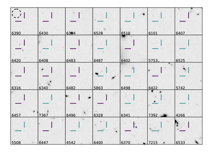
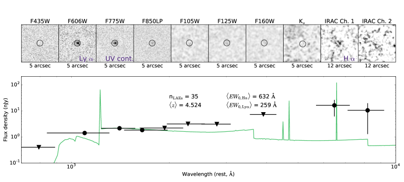
From our candidate sample of 41, we manually remove 6 objects with severely contaminated IRAC photometry, and those sources with significant residual flux in the cleaned images (see Section 2.1). This leaves a final sample of 35 high-EW LAEs with a median redshift of $z=$ 4.52, for which HST/ACS $F775W$ cutouts are shown in Figure 1. This represents 19 per cent of all LAEs in this redshift range from the MUSE UDF catalogs (Inami et al., 2017, and Bacon et al. in prep.). Based on the UV continuum slope measured for these galaxies described in Section 3.4 and the median Lyman-$\alpha$ flux from the PSF-weighted MUSE spectra (which does not include extended emission; Inami et al., 2017), the average rest-frame Lyman-$\alpha$ EW of the sample is 259 Å.

2.1 De-blended IRAC photometry

The large spatial point spread function (PSF) of IRAC (FWHM $\approx$ 2 arcsec) presents a challenge when dealing with compact sources in crowded fields. This is especially true in deep imaging data, where the wings of the PSF from neighboring sources often overlap. To correct for this effect, a higher spatial resolution image can be combined with a model PSF in order to de-blend the photometry in a crowded field. In this case, we use HST $F850LP$ imaging as the high-resolution prior image and follow the procedure of Labbé et al. (2015) and Lam et al. (2019). We create a model IRAC flux distribution for all continuum-detected sources in the field, which we then subtract from the IRAC data. We are therefore left with a residual image that should only contain flux from the primary (continuum-undetected) source

All 12 $\times$ 12 arcsecond cutouts are visually inspected for defects, which can be caused by e.g. poorly-modeled bright sources or can occur in exceptionally crowded fields. Any object that is deemed to have contaminated photometry due to model residuals is removed from the sample. We note that these contamination effects are independent of the intrinsic properties of the primary source. The resulting “clean” sample has residuals in the range of 0.01 to 0.3 nJy (cf. the mean from the “contaminated” sources of 0.6 nJy), determined via the standard deviation of pixel values within an annular region centred on the source and extending from 1.5 to 3 arcseconds.

3 Determination of $\xi_{ion}$

The three ingredients required to measure $\xi_{\mathrm{ion}}$ are the flux of H $\alpha$ (a proxy for the intrinsic ionizing photon production rate), the flux of the UV, and the escape fraction of ionizing photons:

$$\xi_{\textrm{ion}}(\textrm{Hz erg}^{-1})=Q(H^{0})/L_{\textrm{UV,int}}$$ (1)

where $Q(H^{0})$ is the intrinsic rate of ionizing photons with units of s^-1 and the intrinsic UV luminosity, $L_{\textrm{UV,int}}$, has units of erg s^-1 Hz^-1. Below we outline the determinations of each of these quantities from our data.

3.1 H $\alpha$ from IRAC stacking

We create a three-dimensional array of the cleaned IRAC cutouts for the LAEs, each of which are centered on the peak of the Lyman-$\alpha$ flux. We calculate the mean of the array at each spatial pixel, incorporating a sigma-clipping procedure with a threshold of 2-$\sigma$ in order to ensure that individual bright pixels do not dominate the mean. This “stacking” procedure results in a two-dimensional image, representing an average of the input sources. As the IRAC PSF varies across the field due to the combined nature of the GREATS dataset (see Section 3.2 of Labbé et al., 2015), we also create a 3D array of the local PSFs at the position of each LAE. This stack of PSFs is combined in the same way as the stack of the science data arrays, using the same mask derived from sigma-clipping. We fit this PSF to the stacked image to determine the total flux, under the assumption that our sources are unresolved compared to the 2 arcsecond IRAC PSF (cf. the HST images). The fit includes uncertainties in the flux determined from stacking the IRAC noise images in the same way as the data. This stacking procedure is used to measure the photometry and create the images shown in Figure 2.

For the remainder of this work, we deal with the distribution of the output IRAC Ch. 1 and Ch. 2 fluxes using random subsets of the 35 individual LAEs. Namely, we create a series of 10,000 data arrays made up of a random set of 35 LAEs, where we sample the full set with replacement. Each of these arrays is analyzed as above to determine flux in Ch. 1 and Ch. 2. This bootstrap procedure allows us to measure the distribution of H $\alpha$ fluxes within the sample while taking into account photometric uncertainties.

We determine the H $\alpha$ fluxes for each of the 10,000 bootstrap iterations by subtracting the Ch. 2 flux from the Ch. 1 flux, assuming Ch. 2 probes the underlying stellar continuum (see Section 3.1.1). We attribute all of the excess flux in Ch.1 to H$\alpha$ emission: in the models of Gutkin et al. (2016), for metallicities $\lesssim$ 10 per cent Z_⊙ the ratio of [N ii] ([S ii]) to H $\alpha$ never exceeds 0.01 (0.1) over a wide range in physical ISM conditions. While a detailed determination of the metallicities of these systems is beyond the scope of this paper and will require additional spectroscopic data, we stress that only models of normal stellar populations with extremely young ages ($<$ 3 Myr) and/or low metallicities ($Z<0.008$; 0.4 Z_⊙) can reproduce such large Lyman-$\alpha$ EWs (Hashimoto et al., 2017a, b, and Section 4). Similar conclusions are drawn by Trainor et al. (2016) for the faintest $z\approx 2.5$ LAEs, where they have spectroscopic access to strong optical emission line ratios.

Figure 2: (Top) Mean-stacked HST, $K_{s}$, and IRAC photometry for the 35 high-EW LAEs in the sample. The HST/$K_{s}$ cutouts are 5 arcseconds on a side, while the IRAC cutouts are 12 arcseconds. The apertures shown are used for the photometric measurements of $M_{\mathrm{UV}}$ from HST (0.4 arcsecond radius). (Bottom) Total observed restframe photometry and sample properties of the high-EW LAEs used in this study, as described in the text. Upper limits (3-$\sigma$) are denoted with downward-facing triangles. For illustrative purposes, we also plot an arbitrarily-scaled theoretical model for a single stellar population 2 Myr after a burst of star formation, with a metallicity of 0.001 (see Section 4 for details). Lines of Hydrogen and Helium are included in the model spectrum, as is the average intergalactic medium transmission at this redshift from Inoue et al. (2014).

3.1.1 The continuum level around H $\alpha$

In order to properly measure the emission line flux from a photometric broad-band measurement, we need to establish the local spectral continuum level. For the aforementioned studies that perform measurements of H $\alpha$ EW at high-$z$, the continuum level at the position of H $\alpha$ is typically established with photometric detections in the bands bluewards/redwards of H $\alpha$, such as the $K_{s}$-band or IRAC Ch. 2. In our case, the ground-based $K_{s}$-band data (from zFOURGE; Straatman et al., 2016) are not deep enough for reliable detections of the continuum flux bluewards of H $\alpha$. As the IRAC Ch. 2 stacks are deeper and are subject to similar systematics as the Ch. 1 data, we use them to constrain the continuum redwards of H $\alpha$ directly.

We assume a flat continuum slope in $f_{\nu}$ (van der Wel et al., 2011). Any residual contamination, if present in both Ch. 1 and Ch. 2, would not bias our determination of the line flux (and hence $\xi_{\mathrm{ion}}$) since this is determined via the difference between both measurements. Furthermore, residual contamination would lower the measured H $\alpha$ EW for a spectrum that is flat in $f_{\nu}$. We also assume no contribution to the Ch. 2 flux from emission lines such as [S iii], which is present for the $z<4.51$ subset of LAEs. As shown in Lam et al. (2019), [S iii] $\lambda$9069 can be strong in LAEs, with EW values in excess of 100 Å. Constraints on [S iii] do not currently exist for galaxies as faint as the LAEs probed here, but at metallicities below 0.3 Z_⊙ the ratio of [S iii] to H $\alpha$ is predicted to be less than 0.05 (Charlot & Longhetti, 2001). Furthermore, any contribution of [S iii] to the IRAC Ch. 2 photometry would mean that we are over-estimating the continuum level and hence under-estimating the strength of H $\alpha$ (and $\xi_{\mathrm{ion}}$).

We determine a mean H $\alpha$ EW for the sample of 632 Å. The 68 per cent confidence interval, weighted by the signal-to-noise of each bootstrap measurement of the H $\alpha$ EW, is between 210 and 1600 Å. The large range in EW measurements is primarily driven by the lower signal-to-noise in the IRAC Ch. 2 stacks, which is typically a factor of 1.9 lower than that derived in IRAC Ch. 1. In the case of measurements at low-EW (i.e. $<$ 210 Å), the typical signal-to-noise in the EW determination is 2.1.

The mean measured star formation rate (SFR) from the H $\alpha$ luminosity is 1.2 M_⊙ yr^-1 (0.4 $-$ 2 M_⊙ yr^-1; 68 per cent) when using the Murphy et al. (2011) conversion. This is larger than the implied UV-based SFR of 0.1 M_⊙ yr^-1, likely due to the fact that H $\alpha$ emission probes star formation on shorter timescales than the UV, namely $<$ 10 Myr, which is important given the implied young ages for these systems: see Section 4.

3.2 UV luminosity from HST stacking

Following the same procedure as for the IRAC stacks, for each bootstrap sample we create stacks of the HST images in order to determine $M_{\mathrm{UV}}$; for more details on this procedure, see Maseda et al. (2018). For the majority of galaxies in our sample, ACS/$F775W$ probes the rest-UV continuum directly. However, for the highest-$z$ objects this band contains flux from Lyman-$\alpha$: 3 of the 35 objects have Lyman-$\alpha$ at a position where the throughput of $F775W$ is greater than 33 per cent. The major results of this paper are consistent within the errors ($<$ 1-$\sigma$) when these higher-$z$ sources are included. Throughout, we assume that $F775W$ probes the UV continuum alone for our sample. Any potential contamination to this flux from Lyman-$\alpha$ emission would mean we are underestimating $\xi_{\mathrm{ion}}$. Additionally, an extrapolation assuming a UV continuum slope of -2.5 from the measured $F850LP$ magnitude is consistent with the measured $F775W$ flux (see Section 3.4). Such a continuum slope is expected for faint LAEs (Hashimoto et al., 2017a), and therefore this implies $F775W$ is a good tracer of the rest-frame UV continuum. We convert the measured $M_{\mathrm{UV}}$ into a luminosity assuming the median redshift for the LAEs in the bootstrap iteration.

3.3 Ionizing photon escape fraction

The escape fraction of ionizing photons relates the observed ionizing photon flux with the intrinsically-produced ionizing photon flux:

$$f_{\mathrm{esc}}^{\mathrm{ion}}=\frac{Q_{\mathrm{obs}}(H^{0})}{Q(H^{0})}.$$ (2)

For brevity, we will refer to $f_{\mathrm{esc}}^{\mathrm{ion}}$ as $f_{\mathrm{esc}}$ throughout the remainder of the text. This parameter is difficult to measure directly as $Q(H^{0})$ is not a readily-observable quantity. Studies such as Ono et al. (2010) suggest using SED fitting to the broadband photometry to estimate $f_{\mathrm{esc}}$ indirectly. At $z=6-7$ they find $f_{\mathrm{esc}}$ to be consistent with zero and constrain it to be $<$ 0.6. Using a similar method, Harikane et al. (2018) fit a relation to $f_{\mathrm{esc}}$ versus EW_Lyα, finding a value consistent with zero for rest-frame EWs in excess of 100 Å. We therefore assume $f_{\mathrm{esc}}$ = 0 throughout, but note that a higher value of $f_{\mathrm{esc}}$ will result in a larger $\xi_{\mathrm{ion}}$.

3.4 Dust attenuation

The true amount of dust extinction in these systems is difficult to establish with SED fitting as even in stacked images we only observe the rest-UV portion of the galaxies in addition to the H $\alpha$ emission. Many studies, particularly at these redshifts $z\approx 4-5$, instead rely on a measurement of the UV continuum slope $\beta$ and assume a dust law, as in Meurer et al. (1999). We measure a median $\beta$ = -2.43 from power-law fits to the rest-UV photometry from each of the bootstrap iterations, with a 68% confidence interval from -3.00 to -2.04, from a power-law fit to the stacked HST photometry for the full stacked sample. We defer a detailed treatment of the $\beta$ slopes of the full sample of high-EW LAEs to a forthcoming paper, but we would like to highlight that the intrinsic stellar UV continuum slope for systems with the highest Lyman-$\alpha$ EWs must be even bluer than the observed value due to the contribution of nebular continuum emission (Raiter et al., 2010).

For $\beta<$ -2.23, Meurer et al. (1999) estimate zero dust correction. As our best-estimate of $\beta$ (and 68 per cent of all bootstrap iterations) is below this, we determine that we do not need to include an additional term for dust attenuation when measuring line fluxes. Although our measurement is uncertain due to the intrinsic faintness of the sample, we a priori expect such a correction to be negligible based on results from (UV-brighter) LAEs at similar or higher redshifts (e.g. Stark et al., 2015; Hashimoto et al., 2017a; Harikane et al., 2018) and the result from Trainor et al. (2016) which shows an anti-correlation between nebular reddening and EW_Lyα. Similarly, Tang et al. (2019) measure the dust attenuation via the Balmer decrement for high-EW [O iii]- and H $\alpha$-emitters, finding negligible extinction for the highest-EW objects. Finally, such a result is also expected when considering the implied low stellar masses and gas-phase metallicities required to power the Lyman-$\alpha$ emission (Garn & Best, 2010).

3.5 The sample distribution of $\xi_{\mathrm{ion}}$

For each bootstrap iteration, we convert the H $\alpha$ flux into a luminosity assuming the median redshift for the LAEs that contributed to the stack. We then convert the luminosity (without a dust correction, as explained above) into the ionizing photon production rate $Q(H^{0})$ assuming Case B recombination at a temperature of 10⁴ K according to:

$$\left[\frac{Q(H^{0})}{\textrm{s}^{-1}}\right]\times(1-f_{\textrm{esc}})=\left(\frac{L_{H\alpha}}{\textrm{erg s}^{-1}}\right)\times 7.37\times 10^{11},$$ (3)

as in e.g. Murphy et al. (2011).

We can therefore calculate $\xi_{\mathrm{ion}}$ according to the usual formula given in Equation 1. The weighted mean of the distribution from the bootstrap iterations assuming zero $f_{\mathrm{esc}}$ is log₁₀ ($\xi_{\mathrm{ion}}$ / Hz erg^-1) $=$ 26.28, with a 68 per cent confidence interval from 25.89 $-$ 26.56, weighted by the individual uncertainties on each measurement.

In Figure 3, we show our estimate of $\xi_{\mathrm{ion}}$ versus $M_{\mathrm{UV}}$, compared to literature samples of line-selected samples (HAEs and LAEs Matthee et al., 2017a; Harikane et al., 2018; Lam et al., 2019) and continuum-selected galaxies (Bouwens et al., 2016) at similar redshifts, as well as “normal” $M_{\star}>10^{9}$ M_⊙, $L\approx$ 0.3$-$3 $L^{\star}$ star-forming galaxies at $z\approx 2$ from Shivaei et al. (2018). We use their value derived from an SMC extinction curve for consistency with the other studies presented here. The bottom panel shows the relationship between the measured luminosities of H $\alpha$ and the rest-frame-UV, which are the two components that go into $\xi_{\mathrm{ion}}$; any trend in $\xi_{\mathrm{ion}}$ versus $M_{\mathrm{UV}}$ could simply be because the UV luminosity goes into both the ordinate and the abcissa. While the information content in both panels is the same, the axes in the top panel are necessarily correlated.

Figure 3: $\xi_{\mathrm{ion}}$ versus $M_{\mathrm{UV}}$ for this sample, emission line-selected literature samples of Matthee et al. (2017a); Harikane et al. (2018); Lam et al. (2019), and the continuum-selected sample of Bouwens et al. (2016). In the case of Shivaei et al. (2018), the dashed line denotes an extrapolation below their faintest bin. The legend describes which result we use from the literature when the authors present multiple values for $\xi_{\mathrm{ion}}$ depending on e.g. their assumed dust law. The error bars on our data points show the (marginalized) sample distribution based on bootstrapping (see Section 3.1), whereas the error bars on $M_{\mathrm{UV}}$ from the literature sample reflect the bin width used in each study. The bottom panel isolates the two individual components of $\xi_{\mathrm{ion}}$, as the axes in the top panel are strongly correlated: the quoted uncertainties in $\xi_{\mathrm{ion}}$ for the literature samples do not typically include the width of the $M_{\mathrm{UV}}$ bins. Our high-EW LAEs are have higher ionizing photon production efficiency for their continuum (UV) luminosity than the literature samples.

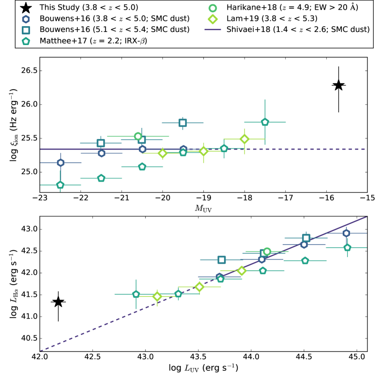
While all of the LAE- and LBG-derived data points are within 2-$\sigma$ (assuming the bin widths correspond to a measurement uncertainty on $L_{\mathrm{UV}}$) of the Shivaei et al. (2018) relation or its extrapolation in either $L_{\mathrm{H\alpha}}$ or $L_{\mathrm{UV}}$, the point derived here is more significantly above the relation for $L_{\mathrm{H\alpha}}$ and $L_{\mathrm{UV}}$. Therefore, relative to their UV luminosity, the MUSE high-EW LAEs are more efficient at producing ionizing photons than the general population of more luminous LBGs and LAEs at these redshifts.

3.6 The Lyman-$\alpha$ escape fraction

As discussed in Section 3.3, it is difficult to directly measure $f_{\mathrm{esc}}$ in these galaxies, although based on other samples we expect it to be low. We can, however, measure the escape fraction of Lyman-$\alpha$ photons:

$$f_{\mathrm{esc}}^{\mathrm{Ly\alpha}}=\frac{L_{\mathrm{Ly\alpha}}^{\mathrm{obs}}}{L_{\mathrm{Ly\alpha}}^{\mathrm{int}}}=\frac{L_{\mathrm{Ly\alpha}}^{\mathrm{obs}}}{8.7\times L_{\mathrm{H\alpha}}^{\mathrm{int}}}$$ (4)

where the superscripts obs and int refer to the observed and intrinsic luminosities, respectively. This equation is valid for Case B recombination with a temperature of 10⁴ K (see Henry et al., 2015; Trainor et al., 2015). Based on our observations, we derive a mean $f_{\mathrm{esc}}^{\mathrm{Ly\alpha}}$value of 0.217, with a 68 per cent confidence interval of 0.067 $-$ 0.333 based on our bootstrap iterations.

4 Discussion

Qualitatively, several studies have found a trend towards having higher $\xi_{\mathrm{ion}}$ values in galaxies with bluer UV continua, a proxy for galaxies with more dominant young stellar populations (Duncan & Conselice, 2015; Bouwens et al., 2015b, 2016). However, Matthee et al. (2017a) show that this is a product of using the UV slope itself (or galaxy SEDs that predominantly trace the rest-UV) as a proxy for dust attenuation. This is also sensitive to the assumed dust model, as can be seen in Figure 4 of Shivaei et al. (2018) where using different dust laws can produce a marginally positive or a negative correlation between $\xi_{\mathrm{ion}}$ and $M_{\mathrm{UV}}$. Nevertheless, Matthee et al. (2017a) find that $\xi_{\mathrm{ion}}$ increases with decreasing UV luminosity, increasing specific star formation rate, and increasing H $\alpha$ EW in their sample of $z\approx 2$ H $\alpha$ emitters.

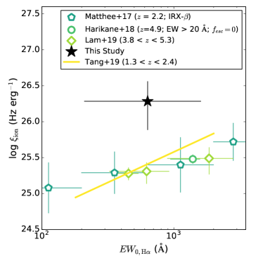
In Figure 4 we compare the equivalent width of H $\alpha$ with the derived $\xi_{\mathrm{ion}}$ value for the emission line-selected samples. In addition, we plot the fit to the relation from Tang et al. (2019) derived from $z\approx 1-2$ “extreme emission line galaxies” (EELGs), which are selected purely on the basis of high-EW optical emission lines ([O iii] and/or H $\alpha$). These systems have gas-phase metallicities $<$ 0.3 Z_⊙ and mass doubling times on the order of 100 Myr (Maseda et al., 2013, 2014). While these physical properties are broadly similar to those of literature samples of LAEs at higher redshifts, the offset compared with the high-EW LAEs presented here argues for a difference in $\xi_{\mathrm{ion}}$ at a fixed age. This is due to the fact that the EW of Balmer lines scales inversely with the age of the stellar population in these types of systems (e.g. van der Wel et al., 2011). Here and throughout, we specifically refer to the light-weighted age, which is dominated by the most recent generation of star formation: an older ($>$ 1 Gyr) stellar population could contribute to the total mass of the galaxy but would not contribute significantly to the UV or H $\alpha$ luminosities. The highest-EW objects in the Tang et al. (2019) sample, with ages $<$ 10 Myr, have the highest values of $\xi_{\mathrm{ion}}$. As these galaxies and the high-EW LAEs presented here have little to no dust attenuation (see Section 3.4), any correlation between $\xi_{\mathrm{ion}}$ and age is not driven by using the rest-UV to correct for dust attenuation. At a fixed H $\alpha$ EW, our sample presents a larger value of $\xi_{\mathrm{ion}}$ than the literature LAE/HAE results, implying a lower gas-phase metallicity. However, in all samples a trend with higher $\xi_{\mathrm{ion}}$ at younger ages is found.

Figure 4: Restframe H $\alpha$ EW versus $\xi_{\mathrm{ion}}$ for this sample, compared to the literature observations of other line emitters (LAEs and HAEs). The error bars are not independent as a higher H $\alpha$ EW necessarily implies a higher $\xi_{\mathrm{ion}}$. The relationship between the EW of H $\alpha$ and $\xi_{\mathrm{ion}}$ is consistent between the literature samples, with a strong trend to higher $\xi_{\mathrm{ion}}$ at higher H $\alpha$ EWs. As the H $\alpha$ EW is inversely proportional to the age, this smooth trend suggests that younger ages are the main driver of elevated $\xi_{\mathrm{ion}}$. Our elevated value at fixed H $\alpha$ EW suggests that these LAEs have a lower (gas-phase) metallicity than other samples presented in the literature (see Figure 5).

Figure 5: Predicted $\xi_{\mathrm{ion}}$ (left), intrinsic Lyman-$\alpha$ EW (i.e. corrected for the Lyman-$\alpha$ escape fraction; centre), and UV continuum slope ($\beta$; right) from the Raiter et al. (2010) stellar population models with constant star formation (solid lines) or an instantaneous burst (dotted lines) at different metallicities (colors), compared to the results presented here. The shaded regions denote our 68 per cent confidence interval in $\xi_{\mathrm{ion}}$ (left), the intrinsic Lyman-$\alpha$ EW for the sample (centre; including the uncertainty on the Lyman-$\alpha$ escape fraction), and $\beta$ (right), all from the bootstrap iterations described in Section 3.1

. We quantify the goodness-of-fit for each combination of star formation history, age, and metallicity in Figure 6.

Figure 6: Scaled likelihood of each of the Raiter et al. (2010) models to reproduce our observations as a function of age and metallicity for a constant star formation history (left) and an instantaneous burst (right). As each combination of metallicity, age, and star formation history produces an estimate for each of our three measured quantities ($\xi_{\mathrm{ion}}$, Lyman-$\alpha$ EW, and $\beta$; Figure 5), we can calculate a likelihood for that combination by comparing the predictions to our posterior probability distributions for each quantity. The total likelihood is then the product of the three individual probabilities, scaled to a maximum of 1. As shown by the colored contours, the most likely models have metallicities of 4$\times$10${}^{-4}~{}-$ 0.008 and ages less than 3 Myr, regardless of the star formation history. We cannot, however, conclusively rule out more metal-poor stellar populations with older ages ($>$ 10 Myr for constant star formation or $>$ 3 Myr for an instantaneous burst).

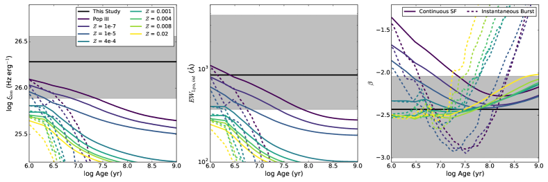
Qualitatively, for a constant star formation history $\xi_{\mathrm{ion}}$ is roughly constant for the first 1 Myr before monotonically declining until the population is approximately 1 Gyr old, when it plateaus again (Figure 5). This is related to differences in the star-formation timescales probed by H $\alpha$ and the UV, and the effect is strongest between 1 and 10 Myr (or longer when binary stellar evolution is included in the models, e.g. Stanway et al., 2016). For an instantaneous burst of star formation, the value of $\xi_{\mathrm{ion}}$ drops strongly after 1 Myr. At a fixed age (and hence UV luminosity) for both star formation histories, decreasing metallicity results in an increasing $\xi_{\mathrm{ion}}$ or H $\alpha$ luminosity. So, while young ages result in higher $\xi_{\mathrm{ion}}$ values for the (bursty) HAEs compared to the general population of star-forming galaxies, the observed offset in $\xi_{\mathrm{ion}}$ at fixed H $\alpha$ EW (and hence fixed age) for the high-EW LAEs shown in Figure 4 suggests that the metallicities must be lower and/or $f_{\mathrm{esc}}^{\mathrm{ion}}$ must be higher. Independent constraints on the metallicity from e.g. rest-optical spectroscopy will be required to determine the contribution of each.

In Figure 5, we show the predictions from the Raiter et al. (2010) stellar population models for the evolution of the H $\alpha$, Lyman-$\alpha$, and UV luminosities at different metallicities for a constant SFR and an instantaneous burst (their “cs5” and “is5” models, respectively). These models use the stellar tracks, atmospheres, and prescriptions for nebular (line and continuum) emission from Schaerer (2003). For the nebular emission, they assume ionization-bounded nebulae with constant electron temperature and densities, and that all photons are absorbed inside the H ii regions (i.e. $f_{\mathrm{esc}}^{\mathrm{ion}}$ $=$ 0). We consider models with a Salpeter (1955) initial mass function, with a high-mass cutoff of 500 M_⊙.

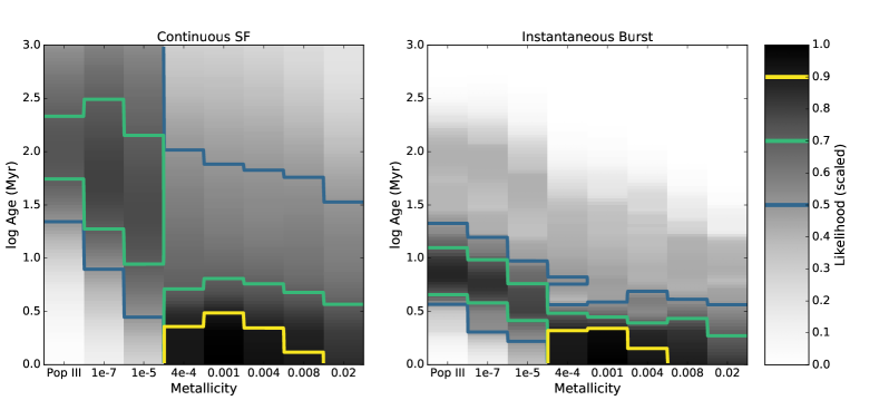
At each age and for a given star formation history, the fixed-metallicity models predict our observable quantities: $\xi_{\mathrm{ion}}$, the EW of Lyman-$\alpha$, and the UV continuum slope $\beta$. We can compare these predicted values to the posterior distributions derived from our bootstrapping procedure and derive a (relative) likelihood for each model. This grid of likelihoods is shown in Figure 6. While we do not have independent constraints on the star formation history, in both cases the most likely models have metallicities of 0.001 (4$\times$10${}^{-4}~{}-$ 0.008) and ages less than 3 Myr. Lower metallicity models are also permitted with older ages, up to 300 Myr. Although the specific metallicity threshold is dependent on our choice of stellar population model and IMF (cf. Stanway et al., 2016), our median value of $\xi_{\mathrm{ion}}$ is difficult to reproduce with any current set of models even when the high-mass cutoff of the IMF is set to 500 M_⊙ (T. Nanayakkara in prep.). This could be related to the lack of very hard ionizing photons in these models which struggle to reproduce observations of high-$z$, low-metallicity galaxies (e.g. Nanayakkara et al., 2019; Kewley et al., 2019).

Trainor et al. (2016) determine a maximum $\xi_{\mathrm{ion}}$ value of $10^{25.6}$ Hz erg^-1 at 7 per cent Z_⊙ from their sample of $z\approx 2.5$ LAEs, some of which have Lyman-$\alpha$ EWs in excess of 100 Å and have UV magnitudes fainter than $-$18. Based on their measurement of a high ionization parameter across their full sample, they conclude that age alone does not drive the elevated $\xi_{\mathrm{ion}}$ that they measure and hence these galaxies should be producing ionizing photons in a steady state. Indeed, even at 100 Myr the models shown in Figure 5 with metallicities below 3 per cent Z_⊙ are elevated with respect to the canonical value. Metallicity can indeed play a role in having an elevated $\xi_{\mathrm{ion}}$, as the extreme Lyman-$\alpha$ EWs require metal-poor ($<$ 0.02 Z_⊙) stellar populations with ages of 10 Myr or less (Figure 5 and Ono et al., 2010; Hashimoto et al., 2017a).

The EW of Lyman-$\alpha$  is observed to scale with $f_{\mathrm{esc}}^{\mathrm{Ly\alpha}}$ (which is correlated with $f_{\mathrm{esc}}^{\mathrm{ion}}$, albeit with large scatter Dijkstra et al., 2016), and for our sample of high-EW LAEs we would expect to have $f_{\mathrm{esc}}^{\mathrm{Ly\alpha}}$ values close to 1 (Sobral & Matthee, 2019). However, we do not observe such large values of $f_{\mathrm{esc}}^{\mathrm{Ly\alpha}}$: as shown in Section 3.6, the mean value is 0.217 assuming Case B recombination (cf. Raiter et al., 2010). This matches the value of 0.3 found in Trainor et al. (2015) despite that sample having a mean Lyman-$\alpha$  EW of only 43 Å. Interestingly, recent observations of an EELG at $z\approx 1.8$ by Erb et al. (2019) find $f_{\mathrm{esc}}^{\mathrm{Ly\alpha}}$to be 0.097, which is also low for its Lyman-$\alpha$ EW. Jaskot et al. (2019) do not find a strong correlation between H $\alpha$ EW, Lyman-$\alpha$ EW, and $f_{\mathrm{esc}}^{\mathrm{Ly\alpha}}$in “green pea galaxies,” which have extreme ionization fields that are plausibly similar to the galaxies presented here. They note that the highest H $\alpha$ EWs reflect high intrinsic Lyman-$\alpha$ production and hence a large escape fraction is not required to produce the observed EWs of Lyman-$\alpha$. In fact, the Sobral & Matthee (2019) model predicts the relationship between $f_{\mathrm{esc}}^{\mathrm{Ly\alpha}}$and the EW of Lyman-$\alpha$ to flatten with increasing $\xi_{\mathrm{ion}}$, such that we could expect a similar value of $f_{\mathrm{esc}}^{\mathrm{Ly\alpha}}$to the one we measure. The extreme galaxies we select here, then, do not require high values of $f_{\mathrm{esc}}^{\mathrm{Ly\alpha}}$ to have the very high EW values measured here (259 Å; median). In addition, Smith et al. (2019) find that the escape of Lyman-$\alpha$ photons lags behind the star formation activity by several tens of Myrs, hence our selection of the youngest star formation episodes via high-EW Lyman-$\alpha$ could preferentially select periods of relatively low escape.

4.1 Alternatives to Star Formation

So far we have only considered star formation as the source of ionizing photons in these systems. Overall, with the current data it is difficult to determine what is the main source of ionizing photons inside these galaxies. As previously mentioned, existing models of normal stellar populations can generally reproduce our observables (i.e. Figure 5). Similar conclusions are drawn by Trainor et al. (2016) for $z\approx$ 3 LAEs, where they use strong optical emission line ratios to demonstrate that star-formation is the dominant source of ionizing photons. In addition, we have demonstrated in Maseda et al. (2018) that the undetected sample plausibly represent the high-EW extension of the distribution of LAEs at these redshifts, a population which is not dominated by AGN.

Thus, we do not believe that AGN are the only or even the dominant contributor to these systems. However, we cannot conclusively rule out some contribution, either as the primary source in a subset of objects or a secondary source in all objects. Further spectroscopy is required in both the restframe-UV and restframe-optical.

5 Outlook and Conclusions

In this work, we have identified a population of 35 $z\approx 4-5$ high-EW LAEs using deep MUSE spectroscopic data in the UDF, with a median Lyman-$\alpha$ EW of 249 Å. By combining this with ultra-deep Spitzer/IRAC photometry, we have measured H $\alpha$ emission with an EW of 632 Å (210 $-$ 1600 Å; 68 per cent) from these systems, and used it to calculate the ionizing photon production efficiency, $\xi_{\mathrm{ion}}$ (Equation 1). Our primary conclusions are as follows:

• Using Spitzer/IRAC photometry to $\approx$ 200 hour depth and sophisticated techniques for source deblending, we detect H $\alpha$ emission in stacked data for objects with intrinsic UV magnitudes fainter than $-$16 (Figure 2).

• The mean value of $\xi_{\mathrm{ion}}$ for these high-EW LAEs is $10^{26.28}$ Hz erg^-1 for an escape fraction of zero, with a 68 per cent confidence interval from $10^{25.89}-10^{26.56}$ Hz erg^-1 (Section 3.5). At a UV magnitude of $-$15.7, this value is a factor of 8.7 in excess of the “canonical” value from literature studies of emission line-selected and continuum-selected samples at similar and higher redshifts, and also higher than the most extreme values for $z\approx 7$ galaxies from Stark et al. (2017) or local galaxies from Chevallard et al. (2018).

• While the values of $\xi_{\mathrm{ion}}$ from the literature are consistent with a constant value at all $M_{\mathrm{UV}}$ (e.g. Lam et al., 2019), our observation lies significantly above this relation (Figure 3). This naturally follows from selecting objects with bright Lyman-$\alpha$ luminosities (and hence ionizing photon production rate) compared to the UV continuum, i.e. selecting on the EW of Lyman-$\alpha$.

• Based on the observed trend between H $\alpha$ EW and $\xi_{\mathrm{ion}}$, as well as models of the evolution of $\xi_{\mathrm{ion}}$ from stellar population synthesis, we determine that an elevated H $\alpha$ luminosity compared with the UV luminosity is likely a natural consequence of a gas-phase metallicity between 4$\times$10^-4 and 0.008 and an age younger than 3 Myr, regardless of the star formation history (Figures 5 and 6).

Typical galaxies selected via the Lyman-break technique (e.g. Bouwens et al., 2017) require detections in the rest-UV, and hence are biased against the youngest ($<$ 10 Myr) galaxies which necessarily have not produced much UV flux. This is true for LAE selections as well (e.g. Lam et al., 2019), even in samples derived from narrow-band imaging (e.g. Harikane et al., 2018), as the relative depth of the emission line detection threshold with respect to the continuum detection threshold prevents these studies from finding the youngest systems. Our MUSE Lyman-$\alpha$ selection, on the other hand, is closer to an H $\alpha$ selection considering it is also a measurement of (emergent) ionizing photons; by requiring non-detections in the rest-frame-UV, we preferentially select the youngest systems. With a selection based on maximal line emission and minimal continuum, it is logical that we have found a population of galaxies with elevated values of $\xi_{\mathrm{ion}}$ compared with older, more massive galaxies.

We expect that observing continuum-faint LAEs with lower line EWs would result in a lower determination of $\xi_{\mathrm{ion}}$ as these systems could have older stellar populations, higher metallicities, or both. Indeed, lower-$z$ observations of $\xi_{\mathrm{ion}}$ show significant scatter at low luminosities and stellar masses (M. Paalvast et al. submitted), which is potentially due to a distribution in the ages, star-formation histories, and metallicities in this regime. These galaxies are currently unobservable in emission at high-$z$, but it is possible to measure the product of $f_{\mathrm{esc}}$ and $\xi_{\mathrm{ion}}$ for systems detected in absorption down to $M_{\mathrm{UV}}$ $\approx$ $-$16 (Meyer et al., 2019) which could select a population of galaxies that are distinct from LAEs.

Various hydrodynamical simulations predict that the star formation histories of low-mass galaxies in the early Universe is episodic in nature, with periods of star formation followed by more quiescent phases (e.g. Shen et al., 2014; Muratov et al., 2015). Although the precise duty cycle of these star formation episodes is unknown and could vary with properties such as the galaxy halo mass (van der Wel et al., 2011), a single galaxy could undergo multiple episodes of efficient ionizing photon production without significantly building up its stellar mass (e.g. Domínguez et al., 2015). Although a phase with extreme Lyman-$\alpha$ EW may not occur during the lifetime of every galaxy, depending on their star formation and metal enrichment histories, all galaxies should produce an excess of ionizing photons at young ages for several Myrs. Further work is required to fully characterize the duty cycle of intense star-formation episodes at high-$z$, but the steep faint-end slope of the UV luminosity function and the observed high number density of high-EW LAEs implies that a significant number of such events should be taking place across cosmic time: at $z=4-5$, high-EW LAEs as selected here represent 6.5 per cent of the full galaxy population at a UV magnitude of $-$16, based on the Bouwens et al. (2015a) luminosity functions. Such a large cumulative number of these episodes could have a significant contribution to cosmic Reionization, especially as LAEs have higher values of $f_{\mathrm{esc}}^{\mathrm{ion}}$ compared to continuum-selected samples (e.g. Trainor et al., 2015; Marchi et al., 2018) and have number densities at $z>6$ that are high enough that they can plausibly contribute significantly to Reionization (Drake et al., 2017). As stated above, understanding the distribution of Lyman-$\alpha$  EWs and the relation between LAEs and the general galaxy population at these redshifts is critical, along with the duty cycle, to fully understand the potential contribution of these faint sources to Reionization.

A detailed discussion of the implications for Reionization is beyond the scope of this work. Many studies combine the measured UV luminosity density $\rho_{\mathrm{UV}}$, derived from UV luminosity functions, with $\xi_{\mathrm{ion}}$ and $f_{\mathrm{esc}}^{\mathrm{ion}}$ in order to infer the ionizing emissivity $\dot{N}_{\mathrm{ion}}$ (e.g. Bouwens et al., 2015b). As we show in Figure 3, $\xi_{\mathrm{ion}}$ can vary with the UV luminosity (e.g. Duncan & Conselice, 2015) and the dust content or metallicity of the galaxy (Shivaei et al., 2018). Additionally, $\rho_{\mathrm{UV}}$ is not well-determined down to $M_{\mathrm{UV}}$ $<-15$ as the majority of the observational constraints come from strong gravitational lensing where the associated systematic uncertainties are large (Bouwens et al., 2017; Atek et al., 2018). Finally, the relationship between LAEs and the general population of galaxies, particularly at these extremely low luminosities, is unclear (e.g. Mesinger et al., 2015).

While these observations are the first step in understanding the ionizing photon production efficiency in such extreme systems, our method necessarily determines the average properties: individual objects could differ significantly. Similar high-EW LAEs at $z<4$ could be studied from the ground in the near-IR with detections of H $\beta$ in extremely long integrations with current instruments, or with future near-IR capabilities provided by the next generation of Extremely Large Telescopes. With the advent of new space-based facilities such as JWST, however, these measurements can be done out to higher redshifts using the brighter H $\alpha$ emission line. Combined with deep rest-UV imaging and spectroscopy to potentially measure $f_{\mathrm{esc}}^{\mathrm{ion}}$, we will obtain a more complete picture of the production and escape of ionizing photons from the abundant low-luminosity population of galaxies in the early Universe.

References

- Atek et al. (2018) Atek H., Richard J., Kneib J.-P., Schaerer D., 2018, MNRAS, 479, 5184
- Bañados et al. (2018) Bañados E., et al., 2018, Nature, 553, 473
- Bacon et al. (2010) Bacon R., et al., 2010, in Ground-based and Airborne Instrumentation for Astronomy III. p. 773508, doi:10.1117/12.856027
- Bacon et al. (2017) Bacon R., et al., 2017, A&A, 608, A1
- Bouwens et al. (2012) Bouwens R. J., et al., 2012, ApJ, 752, L5
- Bouwens et al. (2015a) Bouwens R. J., et al., 2015a, ApJ, 803, 34
- Bouwens et al. (2015b) Bouwens R. J., Illingworth G. D., Oesch P. A., Caruana J., Holwerda B., Smit R., Wilkins S., 2015b, ApJ, 811, 140
- Bouwens et al. (2016) Bouwens R. J., Smit R., Labbé I., Franx M., Caruana J., Oesch P., Stefanon M., Rasappu N., 2016, ApJ, 831, 176
- Bouwens et al. (2017) Bouwens R. J., Oesch P. A., Illingworth G. D., Ellis R. S., Stefanon M., 2017, ApJ, 843, 129
- Charlot & Longhetti (2001) Charlot S., Longhetti M., 2001, MNRAS, 323, 887
- Chevallard et al. (2018) Chevallard J., et al., 2018, MNRAS, 479, 3264
- Dijkstra et al. (2016) Dijkstra M., Gronke M., Venkatesan A., 2016, ApJ, 828, 71
- Domínguez et al. (2015) Domínguez A., Siana B., Brooks A. M., Christensen C. R., Bruzual G., Stark D. P., Alavi A., 2015, MNRAS, 451, 839
- Drake et al. (2017) Drake A. B., et al., 2017, A&A, 608, A6
- Duncan & Conselice (2015) Duncan K., Conselice C. J., 2015, MNRAS, 451, 2030
- Erb et al. (2019) Erb D. K., Berg D. A., Auger M. W., Kaplan D. L., Brammer G., Pettini M., 2019, arXiv e-prints, p. arXiv:1907.11733
- Finkelstein et al. (2012) Finkelstein S. L., et al., 2012, ApJ, 758, 93
- Garn & Best (2010) Garn T., Best P. N., 2010, MNRAS, 409, 421
- González et al. (2012) González V., Bouwens R. J., Labbé I., Illingworth G., Oesch P., Franx M., Magee D., 2012, ApJ, 755, 148
- Gutkin et al. (2016) Gutkin J., Charlot S., Bruzual G., 2016, MNRAS, 462, 1757
- Harikane et al. (2018) Harikane Y., et al., 2018, ApJ, 859, 84
- Hashimoto et al. (2017a) Hashimoto T., et al., 2017a, MNRAS, 465, 1543
- Hashimoto et al. (2017b) Hashimoto T., et al., 2017b, A&A, 608, A10
- Henry et al. (2015) Henry A., Scarlata C., Martin C. L., Erb D., 2015, ApJ, 809, 19
- Illingworth et al. (2013) Illingworth G. D., et al., 2013, ApJS, 209, 6
- Inami et al. (2017) Inami H., et al., 2017, A&A, 608, A2
- Inoue et al. (2014) Inoue A. K., Shimizu I., Iwata I., Tanaka M., 2014, MNRAS, 442, 1805
- Jaskot et al. (2019) Jaskot A. E., Dowd T., Oey M. S., Scarlata C., McKinney J., 2019, arXiv e-prints, p. arXiv:1908.09763
- Kewley et al. (2019) Kewley L. J., Nicholls D. C., Sutherland R. S., 2019, ARA&A, 57, 511
- Labbé et al. (2013) Labbé I., et al., 2013, ApJ, 777, L19
- Labbé et al. (2015) Labbé I., et al., 2015, ApJS, 221, 23
- Lam et al. (2019) Lam D., et al., 2019, A&A, 627, A164
- Marchi et al. (2018) Marchi F., et al., 2018, A&A, 614, A11
- Maseda et al. (2013) Maseda M. V., et al., 2013, ApJ, 778, L22
- Maseda et al. (2014) Maseda M. V., et al., 2014, ApJ, 791, 17
- Maseda et al. (2018) Maseda M. V., et al., 2018, ApJ, 865, L1
- Matthee et al. (2017a) Matthee J., Sobral D., Best P., Khostovan A. A., Oteo I., Bouwens R., Röttgering H., 2017a, MNRAS, 465, 3637
- Matthee et al. (2017b) Matthee J., Sobral D., Darvish B., Santos S., Mobasher B., Paulino-Afonso A., Röttgering H., Alegre L., 2017b, MNRAS, 472, 772
- Mesinger et al. (2015) Mesinger A., Aykutalp A., Vanzella E., Pentericci L., Ferrara A., Dijkstra M., 2015, MNRAS, 446, 566
- Meurer et al. (1999) Meurer G. R., Heckman T. M., Calzetti D., 1999, ApJ, 521, 64
- Meyer et al. (2019) Meyer R. A., Bosman S. E. I., Kakiichi K., Ellis R. S., 2019, MNRAS, 483, 19
- Muratov et al. (2015) Muratov A. L., Kereš D., Faucher-Giguère C.-A., Hopkins P. F., Quataert E., Murray N., 2015, MNRAS, 454, 2691
- Murphy et al. (2011) Murphy E. J., et al., 2011, ApJ, 737, 67
- Nanayakkara et al. (2019) Nanayakkara T., et al., 2019, A&A, 624, A89
- Neufeld (1991) Neufeld D. A., 1991, ApJ, 370, L85
- Oesch et al. (2018) Oesch P. A., et al., 2018, ApJS, 237, 12
- Oke (1974) Oke J. B., 1974, ApJS, 27, 21
- Ono et al. (2010) Ono Y., Ouchi M., Shimasaku K., Dunlop J., Farrah D., McLure R., Okamura S., 2010, ApJ, 724, 1524
- Planck Collaboration et al. (2018) Planck Collaboration et al., 2018, arXiv e-prints, p. arXiv:1807.06209
- Raiter et al. (2010) Raiter A., Schaerer D., Fosbury R. A. E., 2010, A&A, 523, A64
- Rasappu et al. (2016) Rasappu N., Smit R., Labbé I., Bouwens R. J., Stark D. P., Ellis R. S., Oesch P. A., 2016, MNRAS, 461, 3886
- Roberts-Borsani et al. (2016) Roberts-Borsani G. W., et al., 2016, ApJ, 823, 143
- Robertson et al. (2013) Robertson B. E., et al., 2013, ApJ, 768, 71
- Salpeter (1955) Salpeter E. E., 1955, ApJ, 121, 161
- Schaerer (2003) Schaerer D., 2003, A&A, 397, 527
- Shen et al. (2014) Shen S., Madau P., Conroy C., Governato F., Mayer L., 2014, ApJ, 792, 99
- Shim et al. (2011) Shim H., Chary R.-R., Dickinson M., Lin L., Spinrad H., Stern D., Yan C.-H., 2011, ApJ, 738, 69
- Shivaei et al. (2018) Shivaei I., et al., 2018, ApJ, 855, 42
- Smit et al. (2014) Smit R., et al., 2014, ApJ, 784, 58
- Smith et al. (2019) Smith A., Ma X., Bromm V., Finkelstein S. L., Hopkins P. F., Faucher-Giguère C.-A., Kereš D., 2019, MNRAS, 484, 39
- Sobral & Matthee (2019) Sobral D., Matthee J., 2019, A&A, 623, A157
- Stanway et al. (2016) Stanway E. R., Eldridge J. J., Becker G. D., 2016, MNRAS, 456, 485
- Stark et al. (2015) Stark D. P., et al., 2015, MNRAS, 454, 1393
- Stark et al. (2017) Stark D. P., et al., 2017, MNRAS, 464, 469
- Straatman et al. (2016) Straatman C. M. S., et al., 2016, ApJ, 830, 51
- Tang et al. (2019) Tang M., Stark D., Chevallard J., Charlot S., 2019, arXiv e-prints, p. arXiv:1809.09637
- Trainor et al. (2015) Trainor R. F., Steidel C. C., Strom A. L., Rudie G. C., 2015, ApJ, 809, 89
- Trainor et al. (2016) Trainor R. F., Strom A. L., Steidel C. C., Rudie G. C., 2016, ApJ, 832, 171
- Yan & Windhorst (2004) Yan H., Windhorst R. A., 2004, ApJ, 600, L1
- van der Wel et al. (2011) van der Wel A., et al., 2011, ApJ, 742, 111