Physics of Tidal Dissipation in Early-Type Stars and White Dwarfs: Hydrodynamical Simulations of Internal Gravity Wave Breaking in Stellar Envelopes

Abstract

In binaries composed of either early-type stars or white dwarfs, the dominant tidal process involves the excitation of internal gravity waves (IGWs), which propagate towards the stellar surface, and their dissipation via nonlinear wave breaking. We perform 2D hydrodynamical simulations of this wave breaking process in a stratified, isothermal atmosphere. We find that, after an initial transient phase, the dissipation of the IGWs naturally generates a sharp critical layer, separating the lower stationary region (with no mean flow) and the upper “synchronized” region (with the mean flow velocity equal to the horizontal wave phase speed). While the critical layer is steepened by absorption of these waves, it is simultaneously broadened by Kelvin-Helmholtz instabilities such that, in steady state, the critical layer width is determined by the Richardson criterion. We study the absorption and reflection of incident waves off the critical layer and provide analytical formulae describing its long-term evolution. The result of this study is important for characterizing the evolution of tidally heated white dwarfs and other binary stars.

1 Introduction

The physical processes responsible for tidal evolution in close binaries often involve the excitation and dissipation of internal waves, going beyond the “weak friction” of equilibrium tides (see Ogilvie, 2014 for a review). In particular, internal gravity waves (IGWs), arising from buoyancy of stratified stellar fluid, play an important role in several types of binary systems. In solar-type stars with radiative cores and convective envelopes, IGWs are excited by tidal forcing at the radiative-convective boundary and propagate inward; as the wave amplitude grows due to geometric focusing, nonlinear effects can lead to efficient damping of the wave (Goodman & Dickson, 1998; Barker & Ogilvie, 2010; Essick & Weinberg, 2015). In early-type main-sequence stars, with convective cores and radiative envelopes, IGWs are similarly excited at the convective-radiative interface but travel toward the stellar surface; nonlinearity develops as the wave amplitude grows, leading to efficient dissipation (Zahn, 1975, 1977). As the outgoing wave deposits its angular momentum to the stellar surface layer, a critical layer may form and the star is expected to synchronize from outside-in (Goldreich & Nicholson, 1989).

Tidal dissipation can also play an important role in compact double white dwarf (WD) binary systems (with orbital periods in the range of minutes to hours). Such binaries may produce a variety of exotic astrophysical systems and phenomena, ranging from isolated sdB/sdO stars, R CrB stars, AM CVn binaries, high-mass neutron stars and magnetars (created by the accretion-induced collapse of merging WDs), and various optical transients (underluminous supernovae, Ca-rich fast transients, and type Ia supernovae) (e.g. Livio & Mazzali, 2018; Toloza et al., 2019). The outcomes of WD mergers depend on the WD masses and composition, but tidal dissipation can strongly affect the pre-merger conditions of the WDs and therefore the merger outcomes. Tidal dissipation may also influence the evolution of eccentric WD-massive black hole binaries prior to the eventual tidal disruption of the WD (Vick et al., 2017).

Recent studies have identified nonlinear dissipation of IGWs as the key tidal process in compact WD binaries (Fuller & Lai, 2012a; Fuller & Lai, 2013; Fuller & Lai, 2012b; Burkart et al., 2013): IGWs are tidally excited mainly at the composition transitions of the WD envelope; as these waves propagate outwards towards the WD surface, they grow in amplitude until they break, and transfer both energy and angular momentum from the binary orbit to the outer envelope of the WD. However, these previous works parameterized the wave breaking process in an ad hoc manner. The details of dissipation, namely the location and spatial extent of the wave breaking, affect the observable outcomes: dissipation near the surface of the WD can be efficiently radiated away and simply brightens the WD, while dissipation deep in the WD envelope causes an energy buildup that results in energetic flares (Fuller & Lai, 2012b). An important goal of this paper is to elucidate the details of the nonlinear IGW breaking process; the result of this “microphysics” study will help determine the thermal evolution and the observational manifestations of tidally heated binary WDs.

In this paper, we perform numerical simulations of IGW breaking in a plane-parallel stratified atmosphere (a simple model for a stellar envelope). We use the pseudo-spectral code Dedalus (Burns et al., 2016; Burns et al., 2019) and a 2D Cartesian geometry, and consider IGWs propagating into an isothermal fluid initially at rest. We find that, after an initial transient phase, a critical layer naturally develops, separating a lower zone that has no horizontal mean flow and an upper zone with mean flow at the horizontal phase velocity of the IGW. The major part of our paper is dedicated to characterizing the behavior of the critical layer when interacting with a continuous train of IGW excited from the bottom of the atmosphere. IGWs are generally anti-diffusive, in that they steepen shear flows (Lindzen & Holton, 1968; Couston et al., 2018) and act to narrow the critical layer. We find this steepening is counter-balanced by the Kelvin-Helmholtz instability and turbulence within the narrow critical layer. By careful accounting of the momentum flux budget about the critical layer, we are able to model the reflection and absorption of the incident IGW, and the slow downward propagation of the critical layer.

While the motivation of our study is to understand tidal dissipation in WD and early-type stellar binaries, the IGW breaking process studied in this paper is also quite relevant to the circulation dynamics of planetary atmospheres (see e.g. Lindzen, 1981; Holton, 1983; Baldwin et al., 2001).

This paper is organized as follows. In Section 2 we present the system of equations used in our simulations. In Section 3, we review the existing understanding of wave breaking and present analytical results characterizing IGW behavior near a critical layer. In Section 4 we describe our numerical setup and in Section 5 we validate our method in the weak-forcing limit against linear theory. In Section 6, we present the results of simulations of IGW breaking and our characterization of the critical layer. We summarize and conclude in Section 7.

2 Problem Setup and Equations

We consider a incompressible, isothermally stratified fluid representing a stellar envelope or atmosphere. We study dynamics in 2D, so that fluid variables depend only on the Cartesian coordinates $x$ and $z$. While it is well known that waves break differently in 2D versus 3D (Klostermeyer, 1991; Winters & D’Asaro, 1994), the dynamical effect of the breaking process is likely to be similar in 2D (Barker & Ogilvie, 2010). We approximate the gravitational field as uniform, pointing in the $(-\hat{\mathbf{z}})$ direction. The plane-parallel approximation is justified since wave breaking generally occurs near the stellar surface. The background density stratification is given by

$$\overline{\rho}=\overline{\rho}_{0}e^{-z/H},$$ (1)

with $\overline{\rho}_{0}$ some reference density. We denote background quantities with overbars and perturbation quantities with primes.

The Euler equations for an incompressible fluid in a uniform gravitational field are

$$\mathbf{\nabla}\cdot\mathbf{u} =0,$$ (2a)

$$\frac{\mathrm{D}\rho}{\mathrm{D}t} =0,$$ (2b)

$$\frac{\mathrm{D}\mathbf{u}}{\mathrm{D}t}+\frac{\mathbf{\nabla}P}{\rho}+g\hat{\mathbf{z}} =0,$$ (2c)

where $\mathrm{D}/\mathrm{D}t=\partial/\partial t\,+\,\left(\mathbf{u}\cdot\mathbf{\nabla}\right)$ is the Lagrangian or material derivative, and $\mathbf{u},\rho,P$ denote the velocity field, density and pressure respectively. The constant gravitational acceleration is $(-g\hat{\mathbf{z}})$. Note that these equations conserve the same wave energy as the commonly used anelastic equations (Ogura & Phillips, 1962; Brown et al., 2012) and thus give the same wave amplitude growth. Appendix A provides a derivation of these equations and justification for using them.

For this isothermal background, hydrostatic equilibrium implies $\overline{P}(z)=\overline{\rho}(z)gH$. We assume there is initially no background flow, so $\mathbf{u}=\mathbf{u}^{\prime}$. Physically, this assumption corresponds to a non-rotating star.

For convenience, we introduce the dimensionless density variable $\Upsilon$ and the reduced pressure $\varpi$ (e.g. Lecoanet et al., 2014) via

$$\Upsilon \equiv\ln\frac{\rho}{\bar{\rho}},$$ (3)

$$\varpi \equiv\frac{P}{\rho}.$$ (4)

These variables automatically enforce $\rho>0$ and eliminate the stiff term $\mathbf{\nabla}P/\rho$ in the Euler equation. In terms of $\Upsilon$ and $\varpi$, the second two equations in (2) become

$$\frac{\mathrm{D}\Upsilon}{\mathrm{D}t}+u_{z}\frac{\partial\ln\overline{\rho}}{\partial z} =0,$$ (5a)

$$\frac{\mathrm{D}\mathbf{u}}{\mathrm{D}t}+\mathbf{\nabla}\varpi+\varpi\mathbf{\nabla}\Upsilon-\frac{\varpi}{H}\hat{\mathbf{z}}+g\hat{\mathbf{z}} =0.$$ (5b)

Hydrostatic equilibrium corresponds to $\Upsilon=0,\overline{\varpi}=gH$.

3 Internal Gravity Waves: Theory

3.1 Linear Analysis

In the small perturbation limit, we may linearize Eq. (5). The resulting equations admit the canonical IGW solution (Drazin, 1977; Dosser & Sutherland, 2011b)

$$u_{z}^{\prime}\left(x,z,t\right)=Ae^{z/2H}\cos\left(k_{x}x+k_{z}z-\omega t\right),$$ (6)

where $A$ is a constant amplitude, and the frequency $\omega$ and the wave number $\left(k_{x},k_{z}\right)$ satisfy the dispersion relation

$$\omega^{2}=\frac{N^{2}k_{x}^{2}}{k_{x}^{2}+k_{z}^{2}+\left(2H\right)^{-2}}.$$ (7)

Our equations are valid in the limit of large sound speed ($c_{s}\to\infty$), in which the Brunt-Väisälä frequency, $N$, is given by

$$N^{2}\equiv g^{2}\left(\frac{\mathrm{d}\rho}{\mathrm{d}P}-\frac{1}{c_{s}^{2}}\right)=\frac{g}{H},$$ (8)

and is constant. Other dynamical quantities are simply related to $u^{\prime}_{z}$.

In the short-wavelength/WKB limit ($\left|k_{z}H\right|\gg 1$), the solution exhibits the following characteristics:

1. The amplitude of the wave grows with $z$ as $e^{z/2H}$. Thus, the linear approximation always breaks down for sufficiently large $z$.

2. The phase and group velocities are given by:

   $$\mathbf{c}_{p} =\left(k_{x}\hat{\mathbf{x}}+k_{z}\hat{\mathbf{z}}\right)\frac{\omega}{k_{x}^{2}+k_{z}^{2}+\left(2H\right)^{-2}},$$ (9)

   $$\mathbf{c}_{g} =N\frac{\left[k_{z}^{2}+\left(2H\right)^{-2}\right]\hat{\mathbf{x}}-\left(k_{x}k_{z}\hat{\mathbf{z}}\right)}{\left[k_{x}^{2}+k_{z}^{2}+\left(2H\right)^{-2}\right]^{3/2}}.$$ (10)

   The additional $\left(2H\right)^{-2}$ term in the denominator accounts for the growing amplitude of the IGW in the $z$ direction (as the $z$ wavenumber is effectively $k_{z}-i/(2H)$). We note $\mathbf{c}_{p}\cdot\mathbf{c}_{g}=\mathcal{O}\left[\left(k_{z}H\right)^{-2}\right]\approx 0$. In the Boussinesq approximation where terms of order $\mathcal{O}\left(H^{-2}\right)$ are ignored, the phase and group velocities are exactly orthogonal (Drazin, 1977; Dosser & Sutherland, 2011a). We use the convention where upward propagating IGW have $c_{g,z}>0$, $k_{z}<0,k_{x}>0$.

3. The averaged horizontal momentum flux $F$ (in the $+\hat{\mathbf{z}}$ direction) carried by the IGW is defined by

   $$F(z,t)\equiv\left\langle\rho u_{x}^{\prime}u_{z}^{\prime}\right\rangle_{x}\equiv\frac{1}{L_{x}}\int_{0}^{L_{x}}\limits\rho u_{x}^{\prime}u_{z}^{\prime}\;\mathrm{d}x.$$ (11)

   The notation $\left\langle\dots\right\rangle_{x}$ denotes averaging over the $x$ direction. For the linear solution (Eq. 6), this evaluates to

   $$F\approx-\frac{A^{2}}{2}\overline{\rho}_{0}\frac{k_{z}}{k_{x}},$$ (12)

   Thus, indeed $F>0$ for an upward propagating IGW ($c_{g,z}>0$).

3.2 Wave Generation

To model continuous excitation of IGWs deep in the stellar envelope propagating towards the surface, we use a volumetric forcing term to excite IGW near the bottom of the simulation domain. Our forcing excites both IGWs propagating upwards, imitating a wave tidally excited deeper in the star, and downwards, which are not physically relevant in binaries. In our simulations, these downward propagating waves are dissipated by a damping zone described in Section 4.2.

As not to interfere with the incompressibility constraint, we force the system on the density equation. We implement forcing with strength $C$ localized around height $z_{0}$ with small width $\sigma$ by replacing Eq. (5a) with

$$\frac{\mathrm{D}\Upsilon}{\mathrm{D}t}+u_{z}\frac{\partial\ln\overline{\rho}}{\partial z}=Ce^{-\frac{(z-z_{0})^{2}}{2\sigma^{2}}}\cos\left(k_{x}x-\omega t\right).$$ (13)

Using a narrow Gaussian profile excites a broad $z$ power spectrum, but only the $k_{z}$ satisfying the dispersion relation (Eq. 7) for the given $k_{x}$ and $\omega$ will propagate.

In the linearized system, the effect of this forcing can be solved exactly (see Appendix B). In the limit $\left|k_{z}H\right|\gg 1,\sigma\ll H$, the solution can be approximated as two plane waves propagating away from the forcing zone

$$u_{z} (x,z,t)\approx{}\frac{C}{2k_{z}}\frac{gk_{x}^{2}}{\omega^{2}}\exp\left(-\frac{k_{z}^{2}\sigma^{2}}{2}\right)\sqrt{2\pi\sigma^{2}}$$

$${}\times\begin{cases}e^{\frac{z-z_{0}}{2H}}\sin\left(k_{x}x+k_{z}(z-z_{0})-\omega t+\frac{k_{z}\sigma^{2}}{2H}\right)&\text{for }z>z_{0},\\[5.0pt] e^{\frac{z-z_{0}}{2H}}\sin\left(k_{x}x-k_{z}(z-z_{0})-\omega t+\frac{k_{z}\sigma^{2}}{2H}\right)&\text{for }z<z_{0}.\\ \end{cases}$$ (14)

The $z>z_{0}$ region contains an upward propagating IGW wavetrain. The $x$ component of the velocity can be obtained by the incompressibility constraint (Eq. 2a).

3.3 Wave Breaking Height

As the upward propagating IGW grows in amplitude ($\left|\mathbf{u}\right|\propto e^{z/2H}$), it is expected to break due to nonlinear effects. We can estimate the height of wave breaking using the condition $\left|\mathbf{u}\right|\sim\omega/\left|\mathbf{k}\right|$. This can be rewritten using the Lagrangian displacement $\boldsymbol{\xi}=\mathbf{u}/\left(-i\omega\right)$:

$$\left|\xi_{z}k_{z}\right|\sim 1.$$ (15)

Drazin (1977); Klostermeyer (1991); Winters & D’Asaro (1994) describe the onset of wave breaking in some detail. At intermediate amplitudes, wave breaking occurs via triadic resonances, transferring energy from the “parent” IGW to “daughter” waves on smaller length scales that efficiently damp. The horizontal momentum flux decreases from $F$ to $0$ over this breaking region. The lost flux is deposited into a horizontal mean flow

$$\overline{U}(z,t)\equiv\left\langle u_{x}\right\rangle_{x}.$$ (16)

As the mean flow grows, a critical layer may form, as discussed below.

3.4 Critical Layers

A horizontal shear flow $\overline{U}(z,t)\hat{\mathbf{x}}$ enters the fluid equations via the Lagrangian derivative, which can be decomposed as

$$\frac{\mathrm{D}}{\mathrm{D}t}=\frac{\partial}{\partial t}+\overline{U}\frac{\partial}{\partial x}+\left(\mathbf{u}^{\prime}\cdot\mathbf{\nabla}\right),$$ (17)

where $\mathbf{u}^{\prime}$ is the velocity field without the shear flow. Thus, $\overline{U}$ has the effect of Doppler shifting the time derivative into the frame comoving with the mean flow. If $\overline{U}$ is roughly constant, then the behavior of a linear plane-wave perturbation satisfies the modified dispersion relation

$$\left(\omega-\overline{U}k_{x}\right)^{2}=\frac{N^{2}k_{x}^{2}}{k_{x}^{2}+k_{z}^{2}+\left(2H\right)^{-2}}.$$ (18)

This is just Eq. (7) with $\omega\to\omega-\overline{U}k_{x}$. It is apparent that if $\overline{U}=\overline{U}_{c}$, where

$$\overline{U}_{c}\equiv\frac{\omega}{k_{x}},$$ (19)

then the dispersion relation is singular and the linear solution breaks down. Physically, this corresponds to the Doppler-shifted frequency of the IGW being zero. Anywhere $\overline{U}=\overline{U}_{c}$ is called a critical layer.

The behavior of an IGW incident upon a critical layer was first studied in the inviscid, linear regime in Booker & Bretherton (1967), which found nearly complete absorption of the IGW. The amplitude reflection and transmission coefficients are given by

$$\mathcal{R} =\exp\left(-2\pi\sqrt{\mathrm{Ri}-\frac{1}{4}}\right), \mathcal{T} =\exp\left(-\pi\sqrt{\mathrm{Ri}-\frac{1}{4}}\right),$$ (20)

where $\mathrm{Ri}$ is the local Richardson number evaluated at the critical layer height $z_{c}$:

$$\mathrm{Ri}\equiv\left.\frac{N^{2}}{\left(\partial\overline{U}/\partial z\right)^{2}}\right|_{z_{c}}.$$ (21)

In the $\mathrm{Ri}\gg 1$ limit, $\mathcal{R},\mathcal{T}\ll 1$ and the incident wave is almost completely absorbed. This result also applies to viscous fluids (Hazel, 1967). However, weakly nonlinear theory (Brown & Stewartson, 1982) and numerical simulations (Winters & D’Asaro, 1994) suggest that nonlinear effects may significantly enhance reflection and transmission.

Consider now the long-term evolution of the critical layer due to continuous horizontal momentum transfer by IGWs. Any incident horizontal momentum flux absorbed by the fluid, denoted $F_{a}(t)$, must manifest as additional horizontal momentum of the shear flow. Additionally, as the mean flow $\overline{U}$ cannot grow efficiently above $\overline{U}_{c}$ (due to the breakdown of the linear solution), we assume $\overline{U}$ saturates at $\overline{U}_{c}$, which holds to good accuracy (see Fig. 4). In this case, the critical layer must propagate downward in response to the incident momentum flux. The horizontal momentum of the shear flow satisfies

$$\frac{\partial}{\partial t}\int\limits\overline{\rho}(z)\overline{U}(z,t)\;\mathrm{d}z-F_{a}(t)=0.$$ (22)

Assuming $\overline{U}(z>z_{c})\approx\overline{U}_{c}$ and $\overline{U}(z<z_{c})\approx 0$, this condition becomes

$$-\overline{\rho}(z_{c})\overline{U}_{c}\frac{\mathrm{d}z_{c}}{\mathrm{d}t}=F_{a}(t).$$ (23)

If $F_{a}$ is constant in time, the height of the critical layer $z_{c}(t)$ has analytical solution:

$$z_{c}(t)=-H\ln\left[\exp\left(-\frac{z_{c}(t=0)}{H}\right)+\frac{tF_{a}}{\overline{U}_{c}H\overline{\rho}_{0}}\right],$$ (24)

where $z_{c}(t=0)$ is the initial critical layer height.

4 Numerical Simulation Setup

We use the pseudo-spectral code Dedalus (Burns et al., 2016; Burns et al., 2019) to simulate the excitation and propagation of IGWs (Section 5) as well as their nonlinear breaking and the formation of a critical layer (Section 6).

4.1 Parameter Choices

We solve Eqs. (2a), (5b), and (13) in a Cartesian box with size $L_{x},L_{z}$. We choose periodic boundary conditions in both the $x$ and $z$ direction. To mimic the absence of physical boundaries at the top/bottom of the simulation domain, we damp perturbations to zero near the top/bottom using damping zones (see Section 4.2). We expand all variables as Fourier series with $N_{x}$ and $N_{z}$ modes, and use the $3/2$ dealiasing rule to avoid aliasing errors in the nonlinear terms (Boyd, 2001). We choose $L_{z}=12.5H$ ($z$ runs from $-H$ to $11.5H$), and the lower and upper damping zones are active for $z<0.3H$ and $z>9.5H$ respectively. The forcing (see Eq. (13)) is centered at $z_{0}=2H$ with width $\sigma=0.078H$, sufficiently far from the lower damping zone and permitting sufficient room for the upward propagating wave to grow as $\propto e^{z/2H}$. Finally, we want similar grid spacing in the $x$ and $z$ directions (i.e. $L_{x}/N_{x}\sim L_{z}/N_{z}$), guided by the intuition that turbulence generated by wave breaking is approximately isotropic, so we use $L_{x}=4H$ and $N_{z}/N_{x}=4$.

The time integration uses a split implicit-explicit third-order scheme where certain terms are treated implicitly and the remaining terms are treated explicitly. A third-order, four-stage DIRK-ERK scheme (Ascher et al., 1997) is used with adaptive timesteps computed from the minimum of $0.1/N$ and the advective Courant-Friedrichs-Lewy (CFL) time. The CFL time is given by $\Delta t=0.7\min(\Delta x/u_{x},\Delta z/u_{z})$, where the minimum is taken over every grid point in the domain, and $\Delta x\equiv L_{x}/N_{x}$ and $\Delta z\equiv L_{z}/N_{z}$ are the grid spacings in the $x$ and $z$ directions respectively.

We non-dimensionalize the problem such that $H=N=\rho_{0}=1$. The physics of the simulation is then fixed by the four remaining parameters $k_{x}$, $\omega$, $C$, and the viscosity $\nu$. We describe our choices for these parameters below:

1. $k_{x}$: Tidally excited waves in stars generally have $\ell=2$, corresponding to a horizontal wavenumber $k_{\perp}\sim 1/R$, where $R$ is the radius of the star. We use the smallest wavenumber in our simulation, $k_{x}=2\pi/L_{x}$.

2. $\omega$: We choose $\omega$ by evaluating the dispersion relation $\omega(k_{x},k_{z})$ for a desired $k_{z}$ (see Eq. (7)). We pick $\left|k_{z}H\right|=2\pi$ to ensure the waves are very well resolved in all of our simulations. Note however that tidally forced IGWs typically have $\omega\ll N$, or equivalently $k_{r}/k_{\perp}\sim k_{r}R\gg 1$. This requires $\left|k_{z}H\right|\gtrsim 1$, which is only marginally satisfied in our simulations.

3. $C$: In our weak forcing simulations (Section 5), we first choose the forcing strength $C$ (see Eq. (13)) to be sufficiently weak such that $\left|\xi_{z}k_{z}\right|\ll 1$ is satisfied everywhere in the simulation domain. This constrains $C$ by Eq. (14). In our wave breaking simulations (Section 6), we choose larger $C$.

4. $\nu$: Nonlinear effects transfer wave energy from the injection wavenumber $\mathbf{k}$ to larger wavenumbers. Our spectral method does not have any numerical viscosity, so diffusivity must be introduced into the equations to regularize the systems at large wavenumbers. We add viscosity and diffusivity to the system in a way that conserves horizontal momentum (see Appendix C for details). We define the dimensionless Reynolds number

   $$\mathrm{Re}\equiv\frac{\omega}{\nu k_{z}^{2}}=\frac{\omega}{\nu}\left(\frac{H}{2\pi}\right)^{2}.$$ (25)

   We use $\mathrm{Re}\gg 1$ in our simulations.

Finally, we use initial conditions $\mathbf{u}(x,z,0)=\Upsilon(x,z,0)=0$ and $\varpi(x,z,0)=1$, corresponding to hydrostatic equilibrium and no initial fluid motion.

4.2 Damping Layers

We aim to damp disturbances that reach the vertical boundaries of the simulation domain without inducing nonphysical reflection. To do so, we replace material derivatives in Eq. (5) with:

$$\frac{\mathrm{D}}{\mathrm{D}t} \to\frac{\mathrm{D}}{\mathrm{D}t}+\Gamma(z),$$ (26)

$$\Gamma(z) =\frac{1}{2\tau}\left[2+\tanh\frac{z-z_{T}}{\Delta z}+\tanh\frac{z_{B}-z}{\Delta z}\right],$$ (27)

where $z_{B}=0.3H$ and $z_{T}=9.5H$ are the boundaries of the lower and upper damping zones respectively. This damps perturbations below $z_{B}$ and above $z_{T}$ with damping time $\tau$ and negligibly affects the dynamics between $z_{B}$ and $z_{T}$. Most importantly, horizontal momentum remains conserved between $z_{B}$ and $z_{T}$, and outgoing boundary conditions are imposed at $z_{B},z_{T}$. We choose the transition width $\Delta z=0.25H$ and damping time $\tau=1/(15N)$. This prescription is similar to Lecoanet et al. (2016) and has the advantage of being smooth, important for spectral methods. Further details of our implementation of the fluid equations in Dedalus are described in Appendix C.

5 Weakly Forced Numerical Simulation

To test our numerical code and implementation, we carry out a simulation in the weakly forced regime with $C=1.64\times 10^{-7}$. According to the linear solution (Eq. (14)), this generates IGW with $\left|\xi_{z}k_{z}\right|\approx 5\times 10^{-5}$ just above the forcing zone. The IGW grows to $\left|\xi_{z}k_{z}\right|\approx 7.4\times 10^{-3}$ at the upper damping zone and satisfies $\left|\xi_{z}k_{z}\right|\ll 1$ in the entire simulation domain. We include a nonzero $\nu$ corresponding to $\mathrm{Re}=10^{7}$.

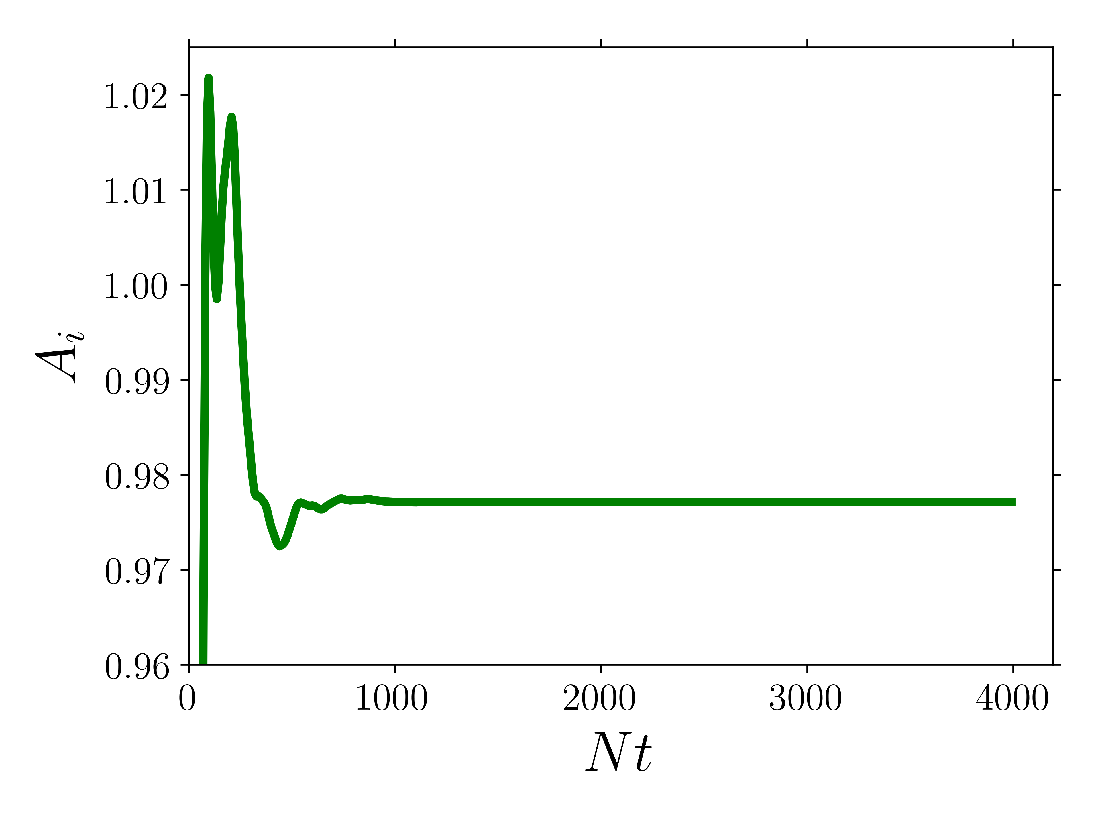
We expect the waves to follow the analytical solution given by Eq. (14) and the corresponding $u_{x}(x,z,t)$; we denote this analytical solution $\mathbf{u}_{an}(x,z,t)$. The amplitude of the observed IGW in the simulation field $\mathbf{u}$ relative to $\mathbf{u}_{an}$ over some region $z\in[z_{b},z_{t}]$ can be estimated from

$$A_{i}(t)=\frac{\int\limits_{z_{b}}^{z_{t}}\int\limits_{0}^{L_{x}}\overline{\rho}\left(\mathbf{u}\cdot\mathbf{u}_{an}\right)\;\mathrm{d}x\mathrm{d}z}{\int\limits_{z_{b}}^{z_{t}}\int\limits_{0}^{L_{x}}\overline{\rho}\left|\mathbf{u}_{an}\right|^{2}\;\mathrm{d}x\mathrm{d}z}.$$ (28)

The subscript $i$ denotes the incident wave. If $\mathbf{u}=\mathbf{u}_{an}$, then $A_{i}(t)=1$. The factor of $\bar{\rho}$ inside the integrands in Eq. (28) corrects for the $\propto e^{z/2H}$ growth of $\mathbf{u}_{an}$; without it, $A_{i}(t)$ would be dominated by the contribution near $z_{t}$.

For the weakly forced simulation, we expect $A_{i}(t)=1$ when integrated between the forcing and damping zones, i.e. $z_{b}\gtrsim z_{0}$ and $z_{t}\lesssim z_{T}$ ($z_{0},z_{T}$ are defined in Eq. (13) and Eq. (27) respectively). For consistency with the nonlinear case later, we choose $z_{b}=z_{0}+3\sigma$ and $z_{t}=z_{b}+H$. Note that using a larger integration domain by choosing $z_{t}=z_{T}-\Delta z$ just below the upper damping zone instead does not change the measured $A_{i}$. The resulting measurement of $A_{i}(t)$ is shown in Fig. 1, and indeed $A_{i}\approx 1$ after the initial transient.

Figure 1: Amplitude of the excited IGW over time (in units of $N^{-1}$) in the weakly forced simulation, computed using Eq. (28). $A_{i}(t)=1$ corresponds to perfect agreement with the analytical estimate. After an initial transient phase, we observe $A_{i}(t)$ asymptotes to $\approx 1$, implying continuous excitation of identical IGW with the expected amplitude. The small deviation of $A_{i}(t)$ from unity may be due to truncation error in our implicit timestepping scheme, as a relatively large fixed step size $\Delta t=0.1/N$ was used for this simulation.

The analytical theory (Section 3.1) also predicts that the horizontal momentum flux $F(z,t)$ is independent of $z$ between the forcing zone where the wave is generated and the damping zone where it is dissipated. The expected horizontal momentum flux carried by the excited IGW in the linear theory can be computed by simply evaluating Eq. (11) for $\mathbf{u}_{an}$ and is a constant:

$$F_{an}\equiv\left\langle\rho u_{an,x}u_{an,z}\right\rangle_{x}.$$ (29)

Denoting the momentum flux measured in the simulation by $F(z,t)$ (use Eq. (11) with velocities taken from the simulation), we expect $F(z,t)=F_{an}$ between $z_{0}$ and $z_{T}$. Fig. 2 shows agreement with this prediction.

Figure 2: $F/F_{an}$ plotted at select times $t$ (in units of $N^{-1}$). As the initial transient dies out, $F/F_{an}\approx 1$ to a good approximation above the forcing zone $z>z_{0}=2H$ and below the damping zone $z\lesssim z_{T}=9.5H$. The horizontal momentum flux excited in the forcing zone is transported without loss to the top of the domain, where it is dissipated by the damping zone (see Section 4.2) without reflection.

6 Numerical Simulations of Wave Breaking

To perform simulations of wave breaking phenomena, we use the same setup as described in Section 4 and Section 5 except for different values of $C$ and $\nu$. In particular, we choose $C$ such that $\left|\xi_{z}k_{z}\right|=0.1$ in the forcing zone ($z=z_{0}$). The linear solution predicts $\left|\xi_{z}k_{z}\right|\sim 4.25$ at the upper damping zone $z_{T}$. We choose the viscosity $\nu$ for each resolution to be as small as possible while still resolving the shortest spatial scales of the wave breaking. A table of our simulations can be found in Table 1.

Resolution	$\mathrm{Re}$
$1024\times 4096$	$2048$
$768\times 3072$	$1024$
$512\times 2048$	$512$
$256\times 1024$	$341$
$256\times 1024$	$205$
$256\times 1024$	$146$

Table 1: Spectral resolutions and Reynolds numbers of simulations of wave breaking.

6.1 Numerical Simulation Results

A full video of our simulation with $N_{x}=768$, $N_{z}=3072$, $\mathrm{Re}=1024$ is available online. We take this to be our fiducial simulation for the remainder of this paper, though other simulations show qualitatively similar behavior.

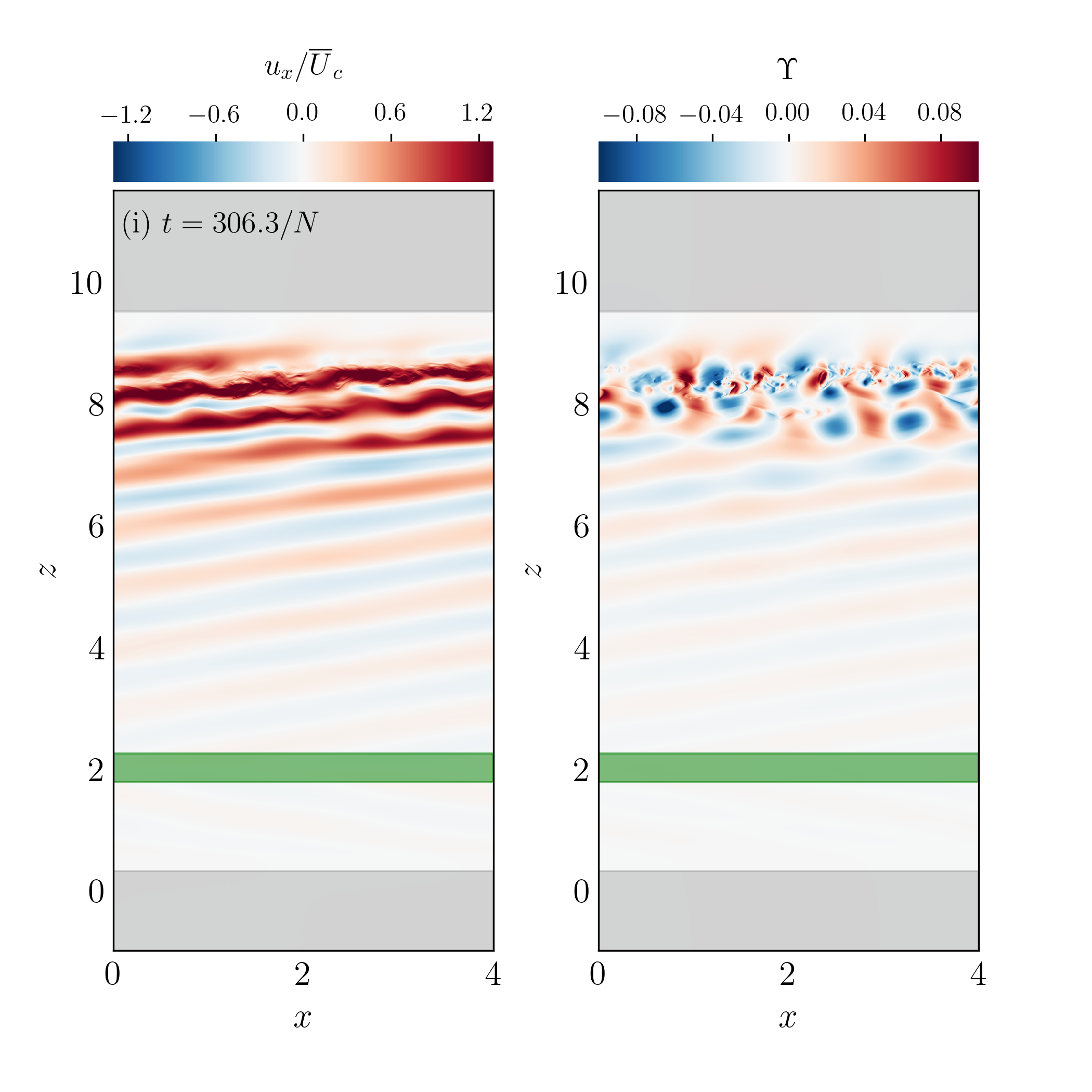
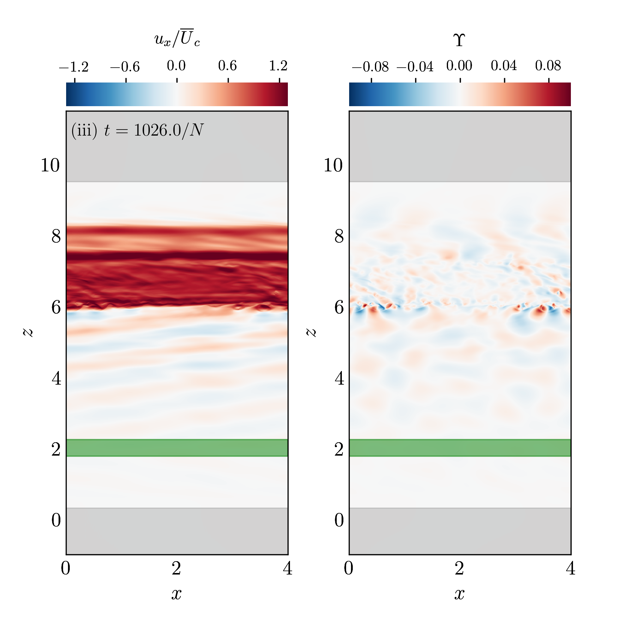
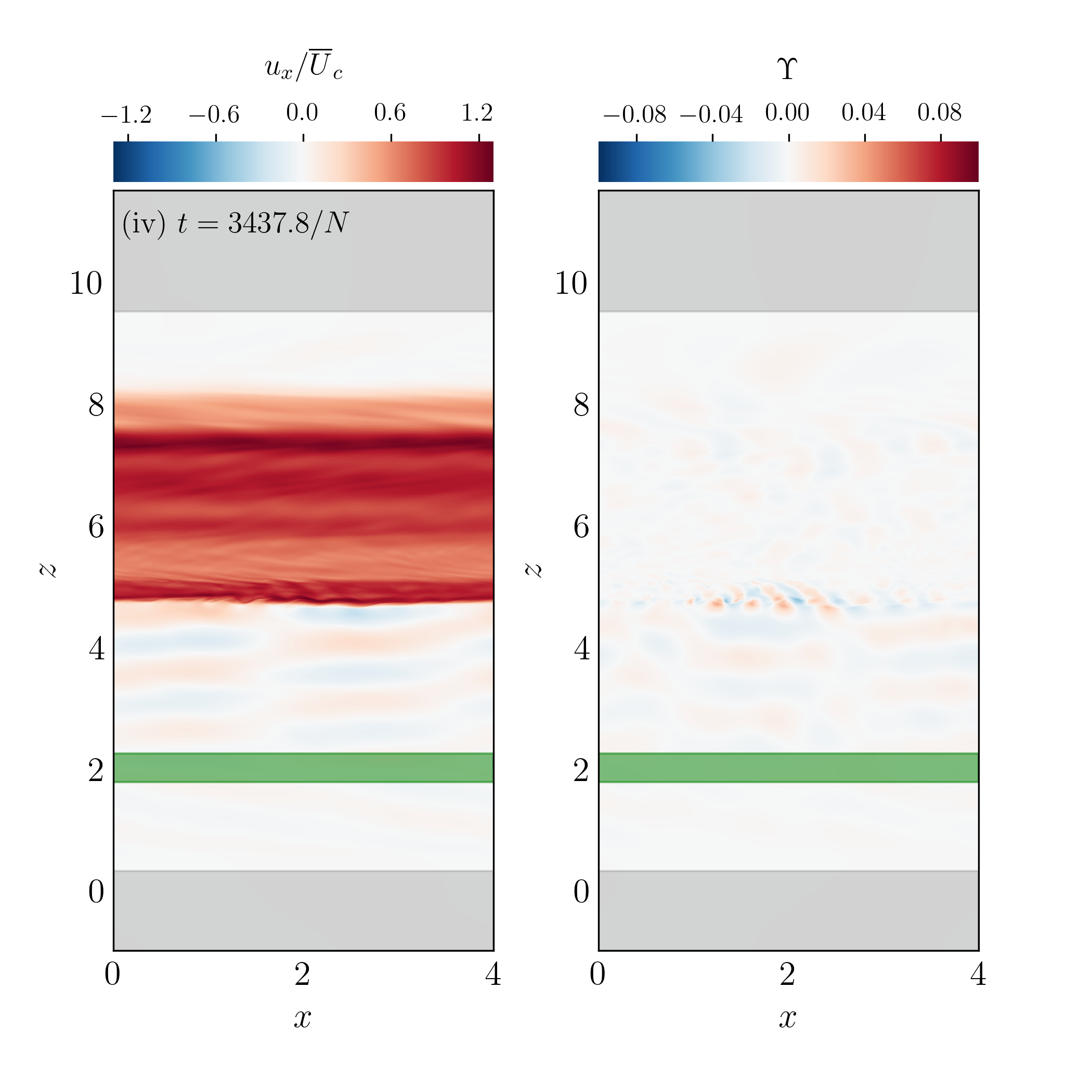
In Fig. 3, we present snapshots of $u_{x}$ and $\Upsilon$ at various phases of the simulation. Note that $\Upsilon\lesssim 0.1$, so the density stratification does not deviate significantly from equilibrium. The flow evolves through several distinct stages:

1. At early times (top left panel), the flow resembles a linear IGW lower in the simulation domain but breaks down into smaller-scale features at higher $z$. Some characteristic swirling motion can be seen in the advected scalar $\Upsilon$, indicating Kelvin-Helmholtz instabilities.

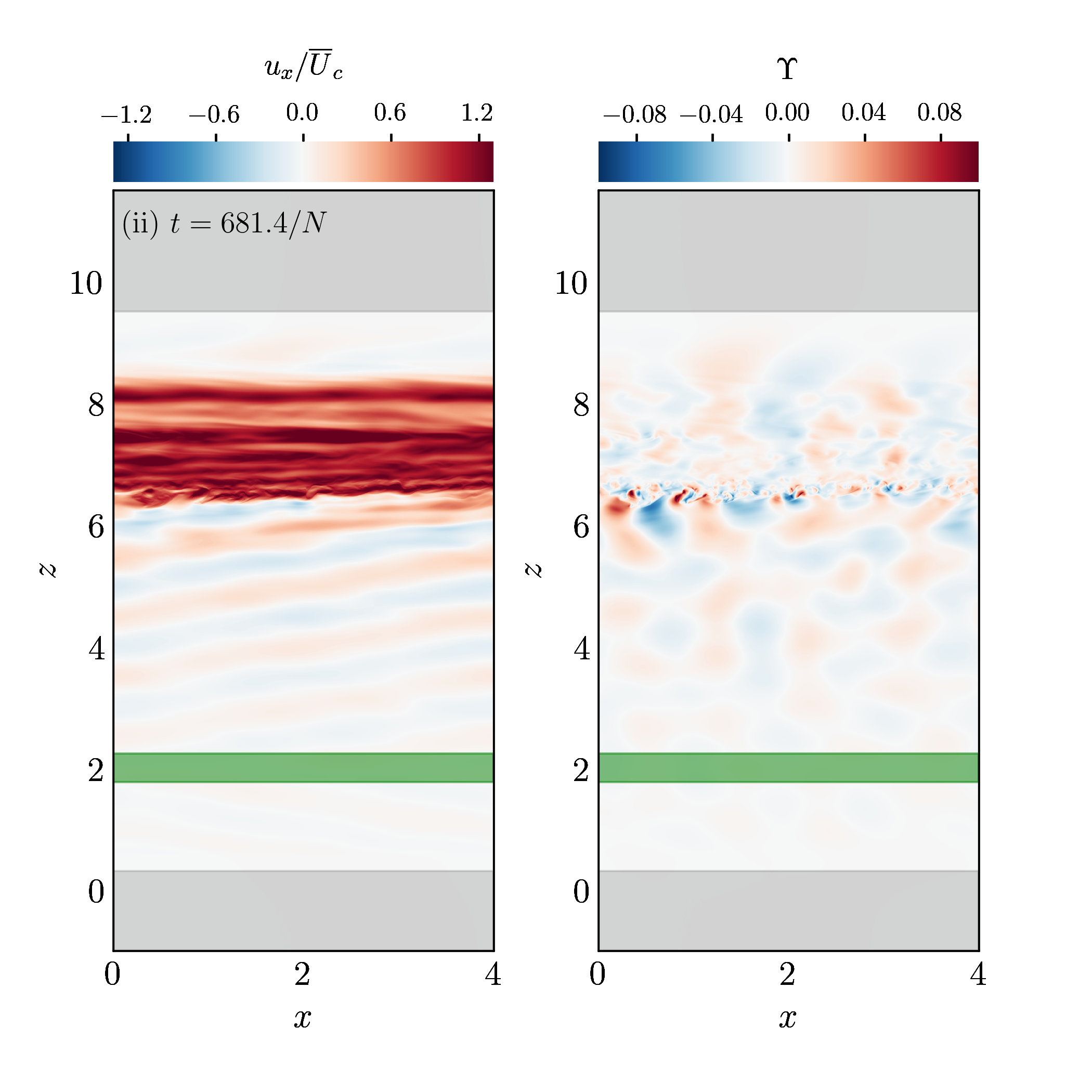
2. At a slightly later time (top right panel), the mean flow in $u_{x}$ becomes much more prominent and the critical layer $z_{c}$ has become much more definite. Small-scale fluctuations are still present in $u_{x}$ but at smaller amplitudes due to being in a denser region of the fluid.

3. In the bottom left panel, the critical layer transition becomes very sharp, and small swirls of limited vertical extent in $\Upsilon$ at the location of the critical layer suggest that the Kelvin-Helmholtz instability is responsible for regulating the width of this transition. More discussion can be found in Section 6.2.

4. At the end of the simulation (bottom right panel), the critical layer has advanced downwards, but otherwise the flow shows very few significant qualitative differences from the previous snapshot. This suggests that the latter phase of the simulation has reached a steady state. Notably, the horizontal banded structure of $u_{x}$ in the upper, synchronized fluid does not continue to evolve (also visible in the top panel of Fig. 4), suggesting that momentum redistribution and mixing within the synchronized fluid are negligible.

Figure 3: Snapshots of $u_{x}$ and $\Upsilon\equiv\ln\left(\rho/\bar{\rho}\right)$ in the fiducial simulation illustrating distinct phases of the evolution of the flow. See the online PDF for a color version. Damping layers at the top and bottom of the simulation domain are shaded in light grey (see Section 4.2), while the forcing zone in the lower middle portion of the simulation domain (see Section 3.2) is shaded in light green (boundaries are at $z_{0}\pm 3\sigma$). The four panels illustrate (i) the initial transient wave breaking phase, (ii) formation of a distinct critical layer, (iii) steepening of the critical layer, and (iv) downward advance of the critical layer.

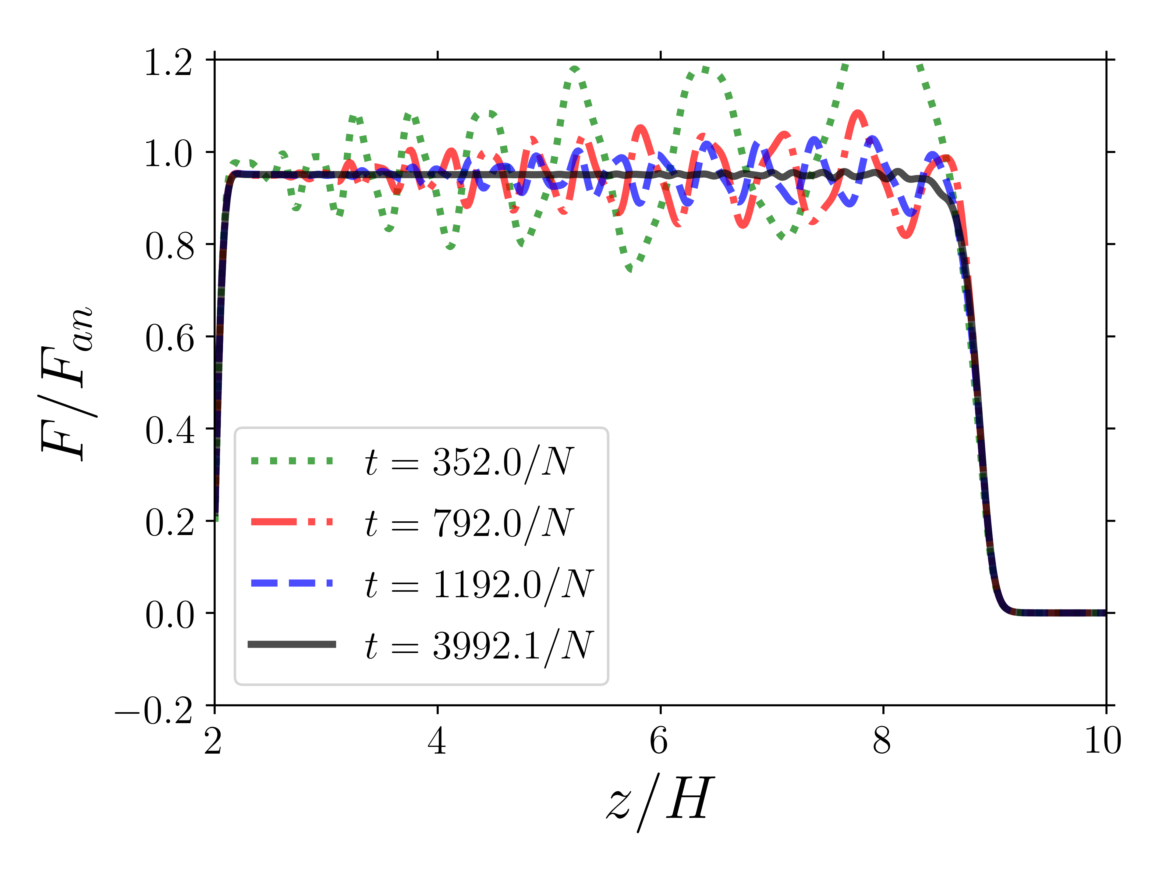
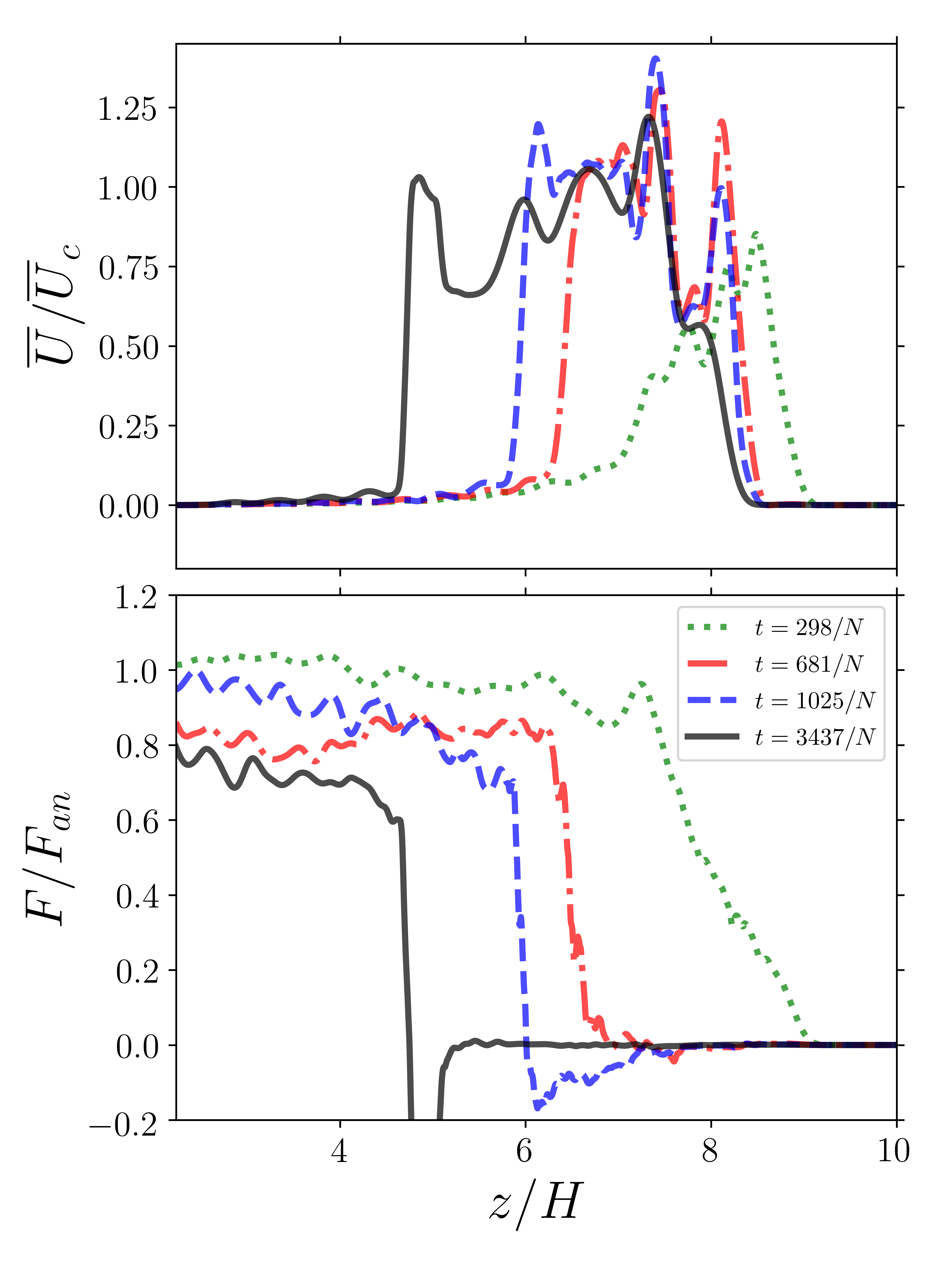
In Fig. 4, we plot the mean horizontal flow velocity $\overline{U}$ (Eq. (16)) and the dimensionless momentum flux $F/F_{an}$ (Eqs. (11) and (29)) as a function of $z$ at the times depicted in Fig. 3. At each time, $\overline{U}$ is close to zero below the critical layer, but then sharply increases to $\overline{U}_{c}$ at the critical layer (i.e. the flow is “spun-up”). Above the critical layer, $\overline{U}$ varies slightly due to momentum transport within the spun-up layer. This agrees with the expectation discussed in Section 3.4.

Similarly, $F\lesssim F_{an}$ below the critical layer, and then decreases to about zero above the critical layer. However, two notable deviations from the discussion in Section 3.4 can be observed: (i) the incident flux on the critical layer fluctuates somewhat temporally, and (ii) there is a small negative flux just above the critical layer at later times. These are addressed in subsequent sections.

Figure 4: The mean horizontal flow velocity $\overline{U}(z,t)$ (Eq. (16)) and the dimensionless momentum flux $F(z,t)/F_{an}$ (Eqs. (11) and (29)) in our fiducial simulation plotted at the same times as in Fig. 3. The two distinct zones of mean flow are separated by a critical layer. The critical layer propagates toward lower $z$ due to momentum transport ($\partial F/\partial z$).

6.2 Kelvin-Helmholtz Instability and Critical Layer Width

The formation of the critical layer is associated with a strong shear flow. What is the width of this layer? Inspection of Fig. 3 suggests the presence of the Kelvin-Helmholtz Instability (KHI) in the critical layer. In a stratified medium, KHI occurs when the Richardson number (Eq. (21)) satisfies $\mathrm{Ri}\lesssim 1/4$ (e.g. Shu, 1991). It is natural to suspect that the shear flow cannot steepen further than the onset of KHI. To test this, we compute the local $\mathrm{Ri}$ for the shear flow around the critical layer.

It is difficult to accurately measure the Richardson number, as it depends on the derivative of the velocity. We measure $\mathrm{Ri}$ as follows: we first assign an $\mathrm{Ri}_{x}(x,t)$ for every $x$ in the critical layer, then take the median of $\mathrm{Ri}$ for the entire layer. $\mathrm{Ri}_{x}$ is computed using the vertical distance over which the local $u_{x}$ increases from $0.3\bar{U}_{c}$ to $\bar{U}_{c}$ (see Eq. (19)). The value $0.3$ is necessary to exclude the small mean flow generated in the weakly nonlinear regime far below the critical layer. This procedure can be written:

$$z_{CL,\min}(x,t) \equiv\min\left\{z\mid u_{x}(x,z,t)>0.3\overline{U}_{c}\right\},$$ (30)

$$z_{CL,\max}(x,t) \equiv\max\left\{z\mid u_{x}(x,z,t)<\overline{U}_{c}\right\},$$ (31)

$$\mathrm{Ri}_{x}(x,t) \equiv\left(\frac{N^{2}\left(z_{CL,\max}-z_{CL,\min}\right)^{2}}{(0.7\overline{U}_{c})^{2}}\right),$$ (32)

$$\mathrm{Ri}(t) \equiv\operatorname*{med}_{x}\mathrm{Ri}\left(x,t\right).$$ (33)

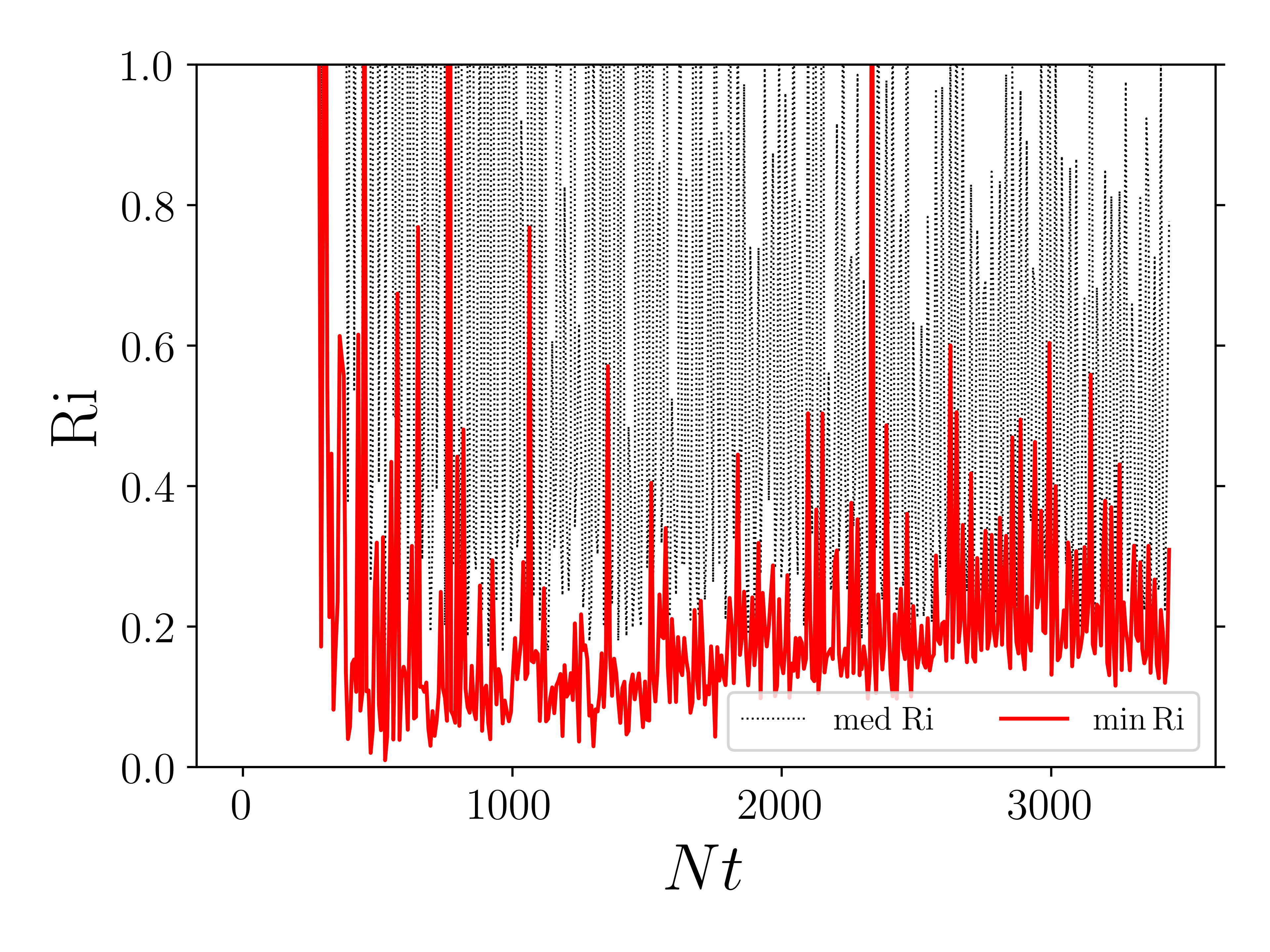
We use the background buoyancy frequency to compute $\mathrm{Ri}$, as fluctuations do not change $N^{2}$ significantly ($\sim 1\%$). To understand the variation in $\mathrm{Ri}$ over $x$, we also compute $\min\limits_{x}\mathrm{Ri}_{x}(x,t)$ (the maximum is very noisy). Both are shown in Fig. 5. Absorption of incident IGWs quickly decreases the Richardson number to between $0.25$ and $0.5$, characteristic of the onset of the KHI.

This result suggests that the critical layer width is regulated by the competition between steepening induced by IGW breaking and broadening due to shear instability. This width does not vary significantly with resolution in our resolved simulations (see Fig. 10). As such, $\mathrm{Ri}\sim 0.5$ can be used to calculate the critical layer width in stars, where $N^{2}$ and $\overline{U}_{c}$ (corresponding to the tidal frequency) are known.

Figure 5: Local Richardson number (Eq. (33)) of the flow at the critical layer over time (in units of $N^{-1}$) in our fiducial simulation. The solid red and dotted black lines denote respectively the minimum and median of $\mathrm{Ri}_{x}(x,t)$. These numbers measure the mean and spread in width of the critical layer over $x$. Note that $\mathrm{Ri}\sim\frac{1}{4}$ corresponds to the KHI, so this plot suggests the shear at the critical layer does not steepen past the onset of the KHI.

6.3 Flux Budget

The downward propagation of the critical layer location $z_{c}(t)$ is driven by the absorption of horizontal momentum flux at $z_{c}$, following Eq. (23). The flux budget at the critical layer can be decomposed as

$$F_{i}(t)=F_{a}(t)+F_{r}(t)+F_{s}(t),$$ (34)

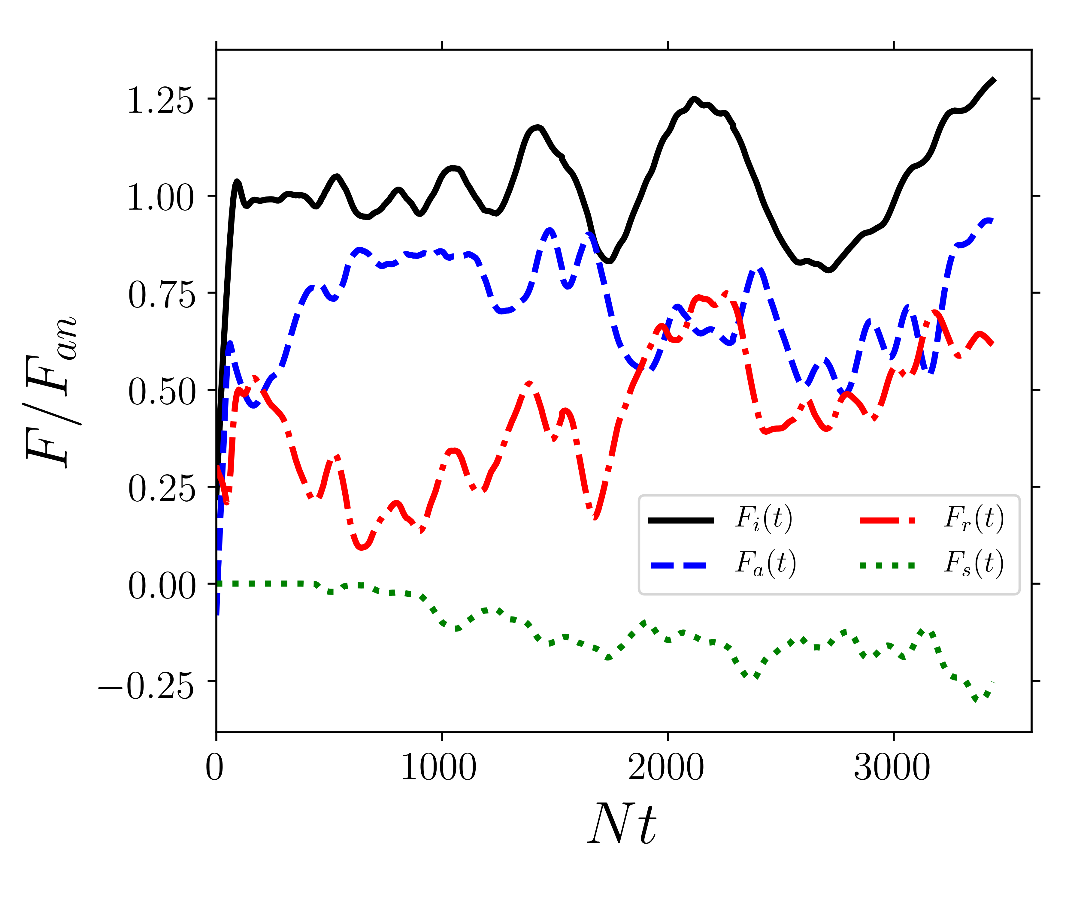
where $F_{i}$ is the incident flux, $F_{a}$ is the absorbed flux, $F_{r}$ is the reflected flux, and $F_{s}$ is some “redistribution” flux above the critical layer, responsible for momentum redistribution within the synchronized upper layer. Careful accounting of $F_{s}$ turns out to be important to obtain the correct $F_{a}$ and resulting critical layer propagation. A more specific physical interpretation of $F_{s}$ is unclear; it is somewhat tempting but unfounded to identify $F_{s}$ with the transmitted flux. In these simulations, we find $F_{s}<0$, corresponding to net momentum transport into the critical layer from the synchronized layer above it.

After measuring $z_{c}$ (see Section 6.4) and $F(z)$ (Eq. (11)) at each time step, we determine each of $F_{i}$, $F_{a}$, $F_{r}$, $F_{s}$ as follows:

$$F_{i}(t) =F_{an}A_{i}^{2}(t),$$ (35)

$$F_{r}(t) =F_{i}(t)-\frac{1}{H}\int\limits_{z_{c}-\Delta z-H}^{z_{c}-\Delta z}F(z,t)\;\mathrm{d}z,$$ (36)

$$F_{s}(t) =\frac{1}{\Delta z}\int\limits_{z_{c}}^{z_{c}+\Delta z}\min(F(z,t),0)\;\mathrm{d}z,$$ (37)

$$F_{a}(t) =F_{i}-F_{r}-F_{s}.$$ (38)

Fig. 6 depicts the four components of this flux decomposition. Below the critical layer, we average over an interval of length $H$, also the vertical wavelength. The offset $\Delta z$ is necessary to make the measurement of the incident flux unaffected by the turbulence within the critical layer itself. The width of the critical layer is limited by $\mathrm{Ri}\lesssim 1$ (see Section 6.2), which bounds its vertical extent $\sim\frac{1}{\left|k_{z}\right|}$. We empirically found an offset of $\Delta z=\frac{3}{\left|k_{z}\right|}$ was necessary to be sufficiently far from strong fluctuations near the critical layer.

Above the critical layer, we observe that the $F_{s}$ feature has varying width (compare e.g. the $t=1171.4/N$ and $t=3437.8/N$ lines in the bottom panel of Fig. 4) but contributes significantly to the total flux budget. We average only where $F<0$ so that $F_{s}$ is robust to such width variations. We find that this is an accurate way of measuring $F_{s}$ and determining $F_{a}$.

Figure 6: Momentum flux decomposition calculated from the simulation. Plotted are the four components of the horizontal momentum flux budget over time (see Eq. (34)), in units of the analytical estimate for the incident wave flux $F_{an}$ (Eq. (12)): $F_{i}$, the flux incident on the critical layer; $F_{a}$, the flux absorbed by the critical layer; $F_{r}$, the flux reflected at the critical layer; and $F_{s}$, the flux inside the synchronized layer.

6.4 Critical Layer Propagation

With a careful determination of $F_{a}$, we can make predictions for the propagation of $z_{c}(t)$ and compare to the measured propagation in the simulation. In principle, $z_{c}$ is the location where the incident flux significantly attenuates. In the simulation, shear turbulence causes $F$ to have significant spatial and temporal fluctuations that translate to large temporal fluctuations in $z_{c}(t)$. To minimize these spurious fluctuations, we measure the location of the critical layer using a spatial average of where flux deposition occurs:

$$z_{c,\min}(t) \equiv\min_{z}\left\{z:F(z,t)>0.3F_{an}\right\},$$ (39)

$$z_{c,\max}(t) \equiv\max_{z}\left\{z:F(z,t)<0.3F_{an}\right\},$$ (40)

$$z_{c}(t) \equiv\frac{z_{c,\min}(t)+z_{c,\max}(t)}{2}.$$ (41)

Measuring $z_{c}$ in other ways does not significantly change the results of the analysis.

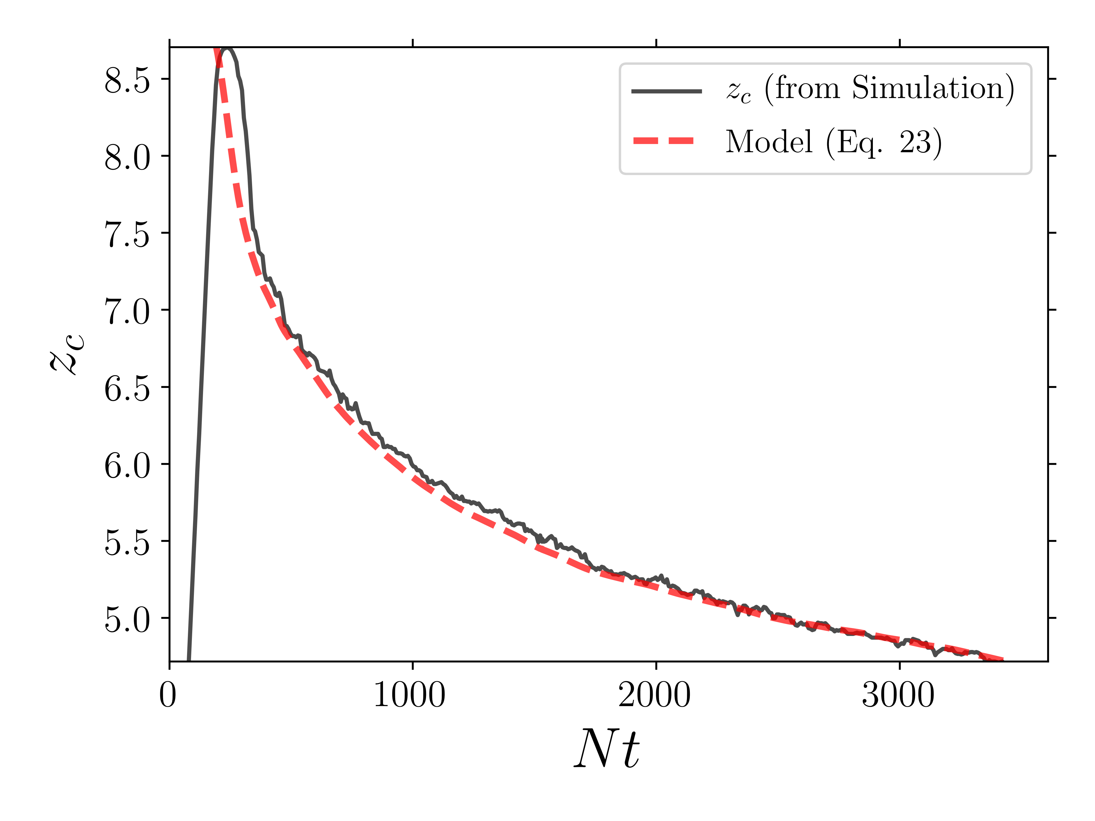
In Fig. 7 we plot the numerically measured $z_{c}$ against numerical integration of Eq. (23) using the measured $F_{a}(t)$. Since the critical layer is still forming at early times, we solve Eq. (23) by integrating backwards from the end of the simulation ($t=t_{f}$), using $z_{c}(t_{f})$ as the initial condition. From Fig. 7, we see that the agreement between the measured $z_{c}(t)$ and its estimate via $F_{a}(t)$ is excellent.

By time-averaging the numerically measured $F_{a}$, we find $\left\langle F_{a}\right\rangle_{t}\approx 0.71F_{an}$. Note that $F_{a}<F_{an}$, so momentum flux absorption at the critical layer is incomplete. This is due to reflection of waves off the critical layer, which carry momentum downward.

Figure 7: Propagation of the critical layer over time. Shown are: (solid black) $z_{c}(t)$ from simulation data, and (dashed red) model for $z_{c}(t)$ using direct integration of Eq. (23) for $F_{a}(t)$ measured from simulation data (described in Eq. (38)). The model uses the end of the simulation as its initial condition and integrates backwards, as the critical layer is still forming at earlier times. The agreement of the model with the simulation shows Eq. (23) is a good description of the evolution of $z_{c}$.

6.5 Non-absorption at Critical Layer

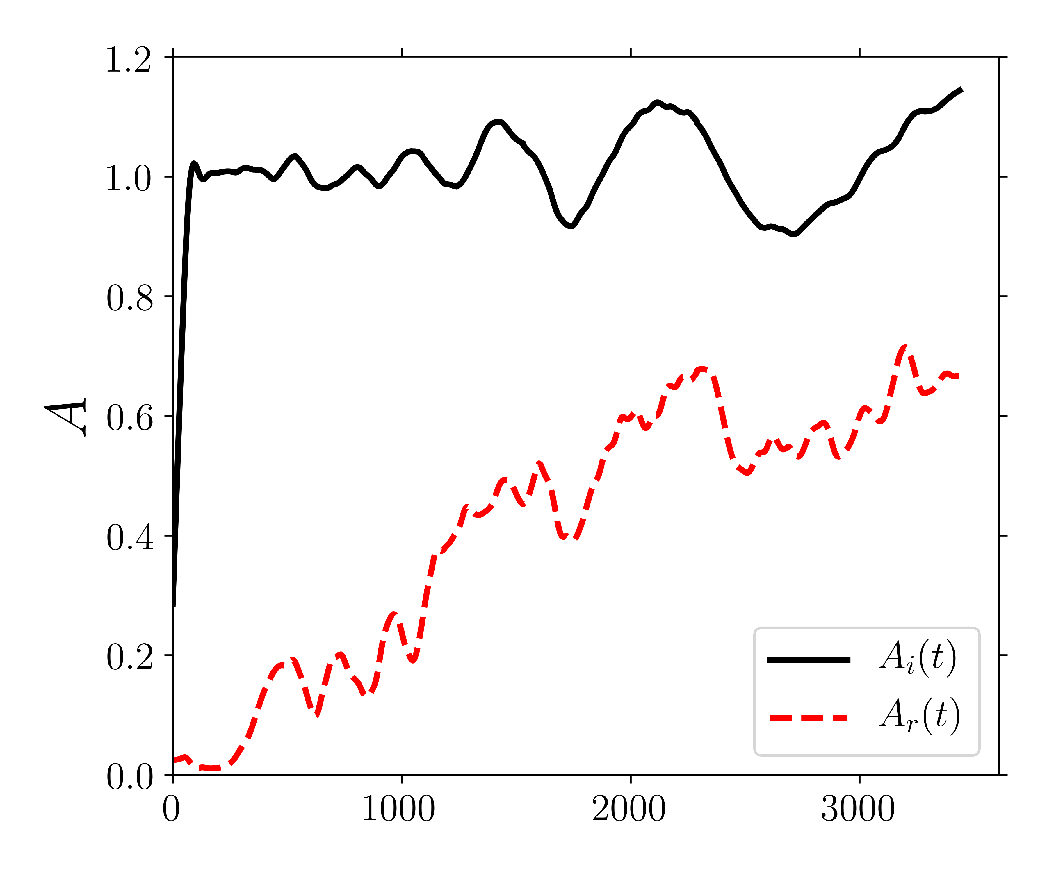
To further understand the behavior at the critical layer, we compare two reflective behaviors observed in the simulation: (i) the presence of a reflected wave with the same frequency as the incident wave (i.e. with wave vector $\mathbf{k}_{r}=k_{x}\hat{\mathbf{x}}-k_{z}\hat{\mathbf{z}}$), and (ii) the reflected flux $F_{r}$. The reflected wave amplitude and flux need not agree exactly if some reflected flux is in higher-order modes, which is indeed the case in our simulations. Both are of physical interest, however: the reflected wave amplitude is essential for setting up standing modes in a realistic star, while the flux is important for accurately tracking angular momentum transfer during synchronization.

To measure the reflected wave amplitude $A_{r}(t)$, we use an approach similar to the calculation of $A_{i}(t)$ (Eq. (28)):

$$A_{r}(t)=\max_{\delta x}\frac{\int\limits_{z_{b}}^{z_{t}}\int\limits_{0}^{L_{x}}\overline{\rho}\left(\mathbf{u}\cdot\left.\mathbf{u}_{an,\mathbf{k}_{r}}\right|_{x=x+\delta x}\right)\;\mathrm{d}x\mathrm{d}z}{\int\limits_{z_{b}}^{z_{t}}\int\limits_{0}^{L_{x}}\overline{\rho}\left|\mathbf{u}_{an}\right|^{2}\;\mathrm{d}x\mathrm{d}z},$$ (42)

where $z_{b}=z_{0}+3\sigma$ and $z_{t}=z_{b}+H$ as before. The primary difference from Eq. (28) is the introduction of free parameter $\delta x$, the horizontal phase offset of the reflected wave. Since $\delta x$ is unknown a priori, we choose $\delta x\in[0,2\pi]$ that maximizes $A_{r}(t)$. In our simulation, the phase offset $\phi_{r}(t)\equiv k_{x}\delta x(t)$ is consistent with reflection off a moving boundary at $z_{c}$, i.e. $\left|\partial\phi_{r}/\partial t\right|\simeq 2\left|\partial(k_{z}z_{c})/\partial t\right|$.

Fig. 8 illustrates the behaviors of $A_{i}$ and $A_{r}$. Both vary significantly in time but their mean values appear to converge towards the end of the simulation.

Figure 8: The incident wave amplitude $A_{i}(t)$ (solid black) and the reflected wave amplitude $A_{r}(t)$ (dashed red) just above the forcing zone.

Since $A_{i}(t),A_{r}(t)$ vary somewhat over time, we perform time averaging over interval of four wave periods, denoted by angle brackets. We can then define the amplitude reflectivity

$$\mathcal{R}_{A}(t)\equiv\frac{\left\langle A_{r}\right\rangle(t)}{\left\langle A_{i}\right\rangle(t)}.$$ (43)

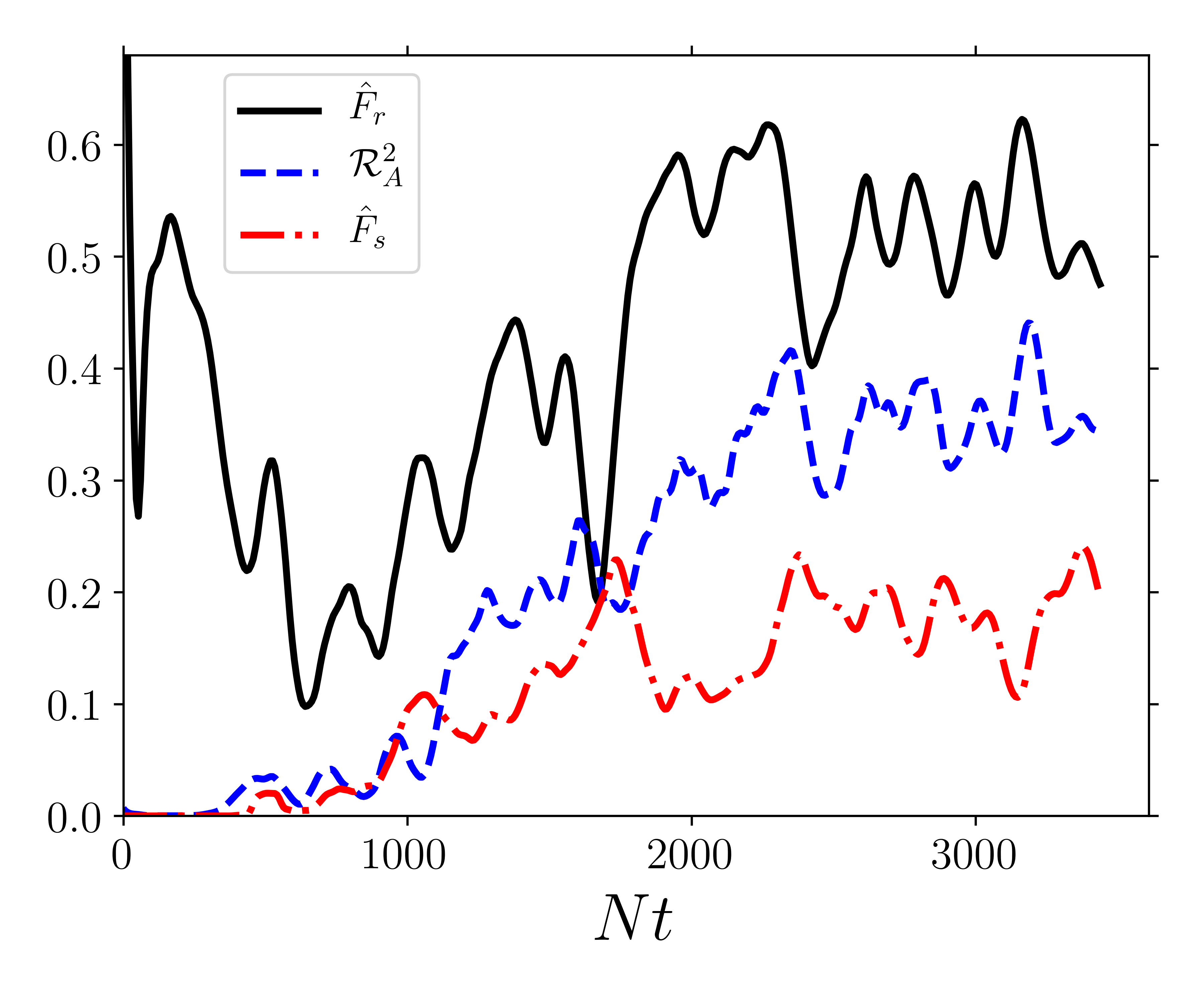
We compare the square of the reflectivity to the ratios of $F_{r}$ and $-F_{s}$ to $F_{i}$, as $F\propto A^{2}$ (Eq. (12)). We define

$$\hat{F}_{r} \equiv\frac{\left\langle F_{r}\right\rangle(t)}{\left\langle F_{i}\right\rangle(t)},$$ (44)

$$\hat{F}_{s} \equiv-\frac{\left\langle F_{s}\right\rangle(t)}{\left\langle F_{i}\right\rangle(t)}.$$ (45)

Fig. 9 shows $\mathcal{R}_{A}^{2}$, $\hat{F}_{r}$, and $\hat{F}_{s}$ as functions of time. The three quantities appear to be roughly stationary for $t\gtrsim 2500/N$. Modest fluctuations ($\sim 20\%$) in $A_{i}$ do not affect our reflectivity results thanks to the time averaging used in Eqs. (43)–(45).We see that in general $\hat{F}_{r}\gtrsim\mathcal{R}_{A}^{2}$, conforming with the expectation that the reflected flux consists of the simple reflected mode and higher order modes as well.

Figure 9: $\mathcal{R}_{A}^{2}$, $\hat{F}_{r}$, and redistribution flux $\hat{F}_{s}$ [Eqs. (43–45)] as a function of time (in units of $N^{-1}$). These quantities seem to become comparatively stable past about $t=2500/N$, indicating that an asymptotic value may have been reached. That $\hat{F}_{r}\gtrsim\mathcal{R}_{A}^{2}$ implies a substantial fraction of reflected flux is in higher-order modes than the reflected IGW.

6.6 Resolution Study

Although throughout this paper we focused on our fiducial simulation with $\mathrm{Re}=1024$ and resolution $N_{x}=768$, $N_{z}=3072$, we also ran a suite of simulations varying the resolution and corresponding Reynolds number (Tab. 1). We find that our global, quantitative measurements in the simulations ($\mathcal{R}_{A}^{2}$, $F_{r}$, $F_{s}$, and $\mathrm{Ri}$) are very similar for our highest Reynolds numbers (1024 and 2048).

For each simulation in Tab. 1, we compute the median values of $\mathcal{R}_{A}^{2}$, $\hat{F}_{r}$, $\hat{F}_{s}$, and $\mathrm{Ri}$ [Eqs. (43–45) and (21) respectively] over the last $1/4$ of the simulation time, when these quantities have reached their asymptotic values. These results are shown in Fig. 10.

Figure 10: Convergence of the median $\hat{F}_{r}$, $\mathcal{R}_{A}^{2}$, $\hat{F}_{s}$, and $\mathrm{Ri}$ (Eqs. (43)–(45) and (21) respectively) in simulations with varying resolution and viscosity as given in Tab. 1. Vertical bars show the temporal variation of each measurement between the $16\%$ and $84\%$ range. Small horizontal displacements are made for data points at identical $\mathrm{Re}$ for readability. Note that simulations with larger $\mathrm{Re}$ correspond to smaller viscosity and are more physically realistic. At the smallest $\mathrm{Re}$ value, $\mathrm{Ri}\approx 50$ is too large to fit on the plot.

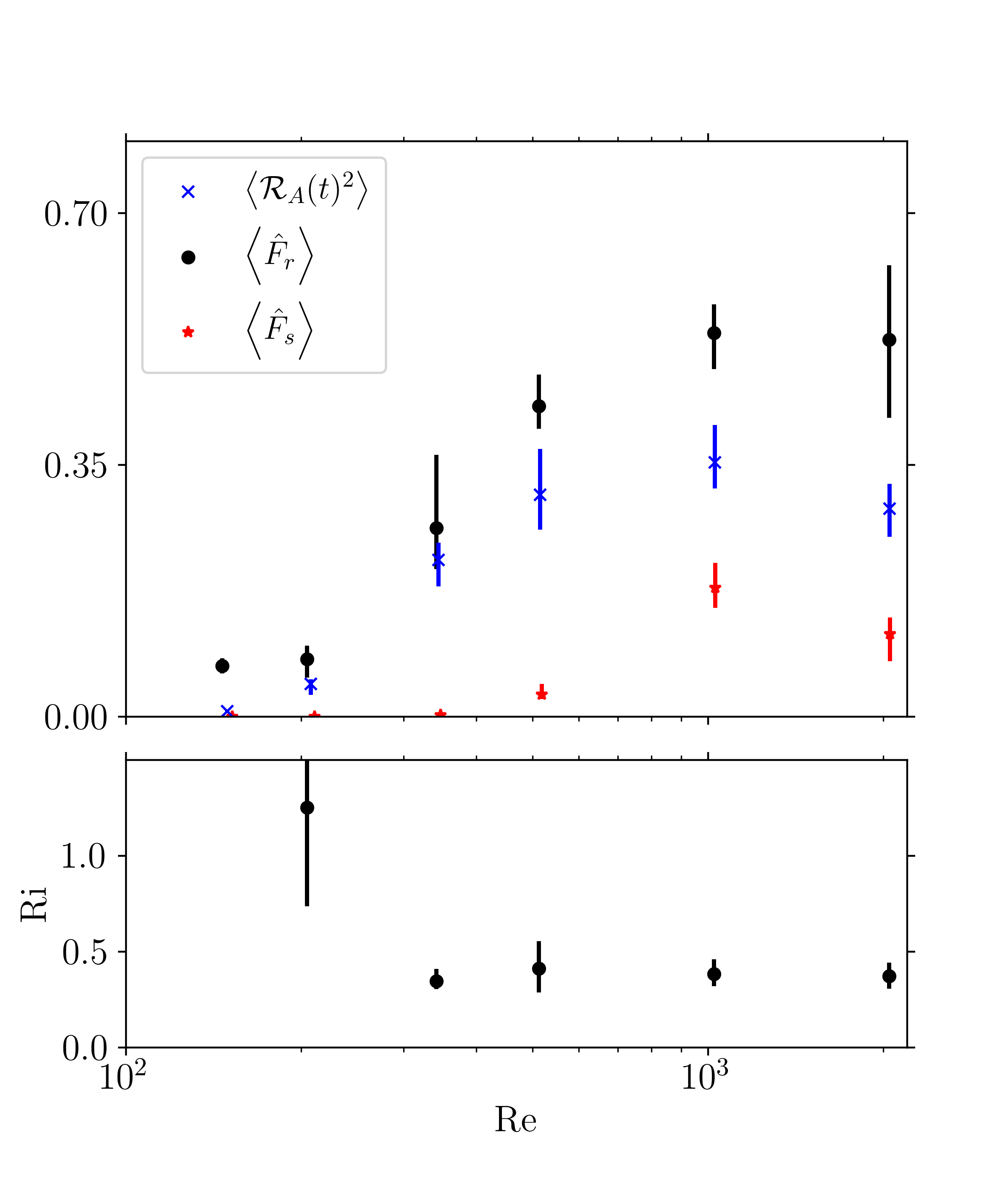
As the simulation resolution increases and the viscosity decreases, we find that the Richardson number decreases, while the reflection and redistribution fluxes increase. The Richardson number is roughly constant for $\mathrm{Re}>200$ with a value of $\mathrm{Ri}\sim 0.4$. The behavior of the fluxes is more complicated. While the fraction of reflected and redistributed flux is similar for our simulations with $\mathrm{Re}=1024$ and $2048$, higher resolution simulations would be required to determine these flux fractions in the limit $\mathrm{Re}\rightarrow\infty$.

Nevertheless, the difference in behavior of $\mathrm{Ri}$ and the flux reflectivity as $\mathrm{Re}$ is varied is in tension with Eq. (20). This tension is natural: Eq. (20) is derived from a linear theory, while fluid motion within the critical layer is turbulent, so reflection at the critical layer cannot be captured by the linear theory.

7 Summary and Discussion

7.1 Key Results

In this paper, we have performed numerical simulations of nonlinear breaking of IGWs in a stratified isothermal atmosphere. Such a setup represents the plane-parallel idealization of the outer stellar envelope. Our simulations use the spectral code Dedalus (Burns et al., 2016; Burns et al., 2019), and are carried out in 2D. We observe spontaneous formation of a critical layer that separates a “synchronized” upper layer of fluid and a lower layer with no mean horizontal flow. This critical layer then propagates downwards as incident IGWs break and deposit horizontal momentum to the fluid (see Fig. 3 for snapshots from our fiducial simulation). Our primary conclusions regarding the evolution of the critical layer are as follows:

1. The width of the turbulent critical layer is determined by requiring the local Richardson number (Eq. (21)) $\mathrm{Ri}\sim 0.5$ (see Fig. 5).

2. The location of the critical layer $z_{c}(t)$ can be predicted by careful measurement of the absorbed horizontal momentum flux at the critical layer (see Eq. (23) and Fig. 7).

3. The absorption of IGW momentum flux at the critical layer is incomplete. The critical layer only absorbs $\sim 70\%$ of the incident flux in our highest resolution simulations (see Fig. 10). The reflected flux is carried away from the critical layer as both lowest-order reflected waves and waves with larger $z$ wavenumbers.

7.2 Discussion

In this paper, we have studied the nonlinear behavior of IGWs with $\left|k_{x}/k_{z}\right|\sim 1/(2\pi)$ in a plane-parallel geometry. Tidally excited IGWs in binary stars have horizontal wavenumber $k_{\perp}\sim 1/R$ (where $R$ is the stellar radius) much smaller than the radial wavenumber $k_{r}$. While our simulations do not satisfy $\left|k_{x}/k_{z}\right|\ll 1$, the qualitative behavior is likely to be similar, as the turbulence driving the critical layer dynamics occurs at scales significantly smaller than either $1/k_{x}$ or $1/\left|k_{z}\right|$. Simulating IGWs with $k_{x}\ll\left|k_{z}\right|$ is more challenging numerically and we defer its exploration to future work.

It is interesting to compare our work with that of Barker & Ogilvie (2010), who studied inward-propagating IGWs in solar-type stars and their nonlinear breaking due to geometric focusing. In their numerical simulations in a 2D polar geometry, they found no evidence for reflected waves, contrary to our result. Note that their simulations were run with substantially higher viscosity, or lower resolution, than explored here, and their effective Reynolds number (equal to $1/\lambda$ in their notation) is of order $10$. We also find at low Reynolds numbers that there is negligible wave reflection.

Regardless of the limitations inherent in our simulations (e.g. plane-parallel geometry), our results shed light on the physical mechanism of tidal heating in close binaries. In particular, our simulations indicate that energy dissipation occurs in a narrow critical layer. The star heats up from outside-in as the critical layer propagates inwards. This tidal heating profile differs flom that used by Fuller & Lai (2012b). We plan to study this issue in a future work.

8 Acknowledgements

This work has been supported in part by the NSF grant AST-17152. YS is supported by the NASA FINESST grant 19-ASTRO19-0041.DL is supported by the Princeton Center for Theoretical Sciences and Lyman Spitzer Jr fellowships. Computations were conducted with support by the NASA High End Computing (HEC) Program through the NASA Advanced Supercomputing (NAS) Division at Ames Research Center on Pleiades with allocation GID s1647.

Appendix A Derivation of Fluid Equations

We aim to model wave dynamics over multiple density and pressure scaleheights. Start with the compressible Euler equations.

$$\partial_{t}\rho+\left(\mathbf{u}\cdot\mathbf{\nabla}\right)\rho+\rho\mathbf{\nabla}\cdot\mathbf{u}=\, 0,$$ (46)

$$\partial_{t}s+\left(\mathbf{u}\cdot\mathbf{\nabla}\right)s=\, 0,$$ (47)

$$\partial_{t}\mathbf{u}+\left(\mathbf{u}\cdot\mathbf{\nabla}\right)\mathbf{u}+\frac{1}{\rho}\mathbf{\nabla}p= \,\mathbf{g},$$ (48)

where $s$ is the entropy. The pressure is calculated from the entropy and density using the equation of state

$$\frac{s}{c_{p}}=\log\frac{p^{1/\gamma}}{\rho},$$ (49)

where $c_{p}$ is the specific heat at constant pressure, and $\gamma$ is the ratio of specific heats. For computational ease, it is convenient to filter out the fast sound waves from these equations. One approach is to assume pressure perturbations are small (yielding the “pseudo-incompressible” equations, Vasil et al., 2013), or that all thermodynamic perturbations are small (yielding the “anelastic” equations, Brown et al., 2012). In these approximations, one of the thermodynamic equations is replaced by a constraint equation: $\mathbf{\nabla}\cdot\left(p_{0}^{1/\gamma}\mathbf{u}\right)=0$ for pseudo-incompressible; $\mathbf{\nabla}\cdot\left(\rho_{0}\mathbf{u}\right)=0$ for anelastic. Here $p_{0}$ and $\rho_{0}$ are the background density and pressure profiles. The pressure in the momentum equation can be interpreted as a Lagrange multiplier which enforces the constraint (Vasil et al., 2013). Upon linearization, both approximations conserve a wave energy

$$E_{w}=\frac{1}{2}\rho_{0}\left|\mathbf{u}\right|^{2}+\frac{1}{2}\frac{g^{2}}{N^{2}}\frac{(\rho^{\prime})^{2}}{\rho_{0}}=\frac{1}{2}\rho_{0}\left|\mathbf{u}\right|^{2}+\frac{1}{2}\rho_{0}N^{2}\frac{(s^{\prime})^{2}}{\left|\mathbf{\nabla}s_{0}\right|^{2}},$$ (50)

where $\rho^{\prime}$ and $s^{\prime}$ represent the density and entropy perturbations.

Rather than assume thermodynamic perturbations are small, we instead filter out sound waves by taking the limit $\gamma\rightarrow\infty$. Then the entropy and log density are proportional to each other, and the entropy equation becomes

$$\partial_{t}\log\rho+\left(\mathbf{u}\cdot\mathbf{\nabla}\right)\log\rho=0.$$ (51)

Together with mass conservation, this implies

$$\mathbf{\nabla}\cdot\mathbf{u}=0.$$ (52)

We solve these equations together with the normal momentum equation.

Although these equations are non-standard, they have various desirable properties. They conserve mass and momentum, and the linearized equations conserve the wave energy $E_{w}$ [Eq. (50) above] similar to the pseudo-incompressible equations and anelastic equations. Our equations also satisfy the same linear dispersion relation as the fully compressible equations in the limit of large sound speed (this is also true for the anelastic equations, but not pseudo-incompressible, Brown et al., 2012; Vasil et al., 2013). Thus, the vertical propagation of internal gravity waves is similar to the pseudo-incompressible equations and anelastic equations.

In this work we are interested in waves which reach large amplitudes and break. For breaking waves, Achatz et al. (2010) suggests that the anelastic equations may miss important effects. Although the pseudo-incompressible equations may capture wave-breaking more accurately, they are more complicated, and do not satisfy the correct dispersion relation to order $(k_{z}H)^{-2}$ (Vasil et al., 2013). In the absence of a clear choice to study this wave breaking problem, we have elected to use these simple equations derived in the $\gamma\rightarrow\infty$ limit.

Appendix B Forcing Solution

To solve for the linear excited IGW amplitude due to bulk forcing (see Eq. (13)), we consider the linearized system of equations, with all dynamical variables having dependence $u_{z}(x,z,t)=\tilde{u_{z}}(z)e^{ik_{x}x-i\omega t}$. Thus, $\partial/\partial t\to-i\omega t$, $\frac{\partial}{\partial x}\to ik_{x}$, and the dynamical fluid equations become (see Eqs. (2) and (5)):

$$\frac{\mathrm{d}u_{z}}{\mathrm{d}z}+ik_{x}u_{x} =0,$$

$$-i\omega u_{x}+ik_{x}\varpi+gHik_{x}\Upsilon =0,$$

$$-i\omega u_{z}+\frac{\mathrm{d}\varpi}{\mathrm{d}z}+gH\frac{\mathrm{d}\Upsilon}{\mathrm{d}z}-\frac{\varpi}{H} =0,$$

$$-i\omega\Upsilon-\frac{u_{z}}{H} =C\exp\left[-\frac{(z-z_{0})^{2}}{2\sigma^{2}}\right]\equiv\mathcal{C}(z).$$

These can be recast solely in terms of $u_{z}$ as

$$\frac{\mathrm{d}^{2}u_{z}}{\mathrm{d}z^{2}}-k_{x}^{2}u_{z}-\frac{1}{H}\frac{\mathrm{d}u_{z}}{\mathrm{d}z}+u_{z}\frac{N^{2}k_{x}^{2}}{\omega^{2}} =-\frac{gk_{x}^{2}}{\omega^{2}}\mathcal{C}(z)..$$

The homogeneous solutions are of form $u_{z,\pm}(z)=\exp\left[\left(\frac{1}{2H}\pm ik_{z}\right)\left(z-z_{0}\right)\right]$ where $k_{z}$ satisfies the dispersion relation (Eq. (7)). We compute the solution to the inhomogeneous ODE by the method of variation of parameters. The Wronskian is

$$W\equiv\det\begin{vmatrix}u_{z,+}&u_{z,-}\\[4.0pt] \mathrm{d}u_{z,+}/\mathrm{d}z&\mathrm{d}u_{z,-}/\mathrm{d}z\end{vmatrix}=-2ik_{z}e^{z/H}.$$ (53)

The general solution is then

$$u_{z}=-u_{z,+}\int\frac{1}{W}u_{z,-}\left(-\frac{gk_{x}^{2}}{\omega^{2}}\mathcal{C}(z)\right)\;\mathrm{d}z+u_{z,-}\int\frac{1}{W}u_{z,+}\left(-\frac{gk_{x}^{2}}{\omega^{2}}\mathcal{C}(z)\right)\;\mathrm{d}z.$$ (54)

Taking these integrals and applying the boundary conditions $u_{z}\left(z\to\infty\right)=u_{z,+}$, $u_{z}\left(z\to-\infty\right)=u_{z,-}$ give the exact solution:

$$u(z) =\frac{\sqrt{\pi}C\sigma}{2^{3/2}ik_{z}}\frac{gk_{x}^{2}}{\omega^{2}}\exp\left[\frac{\left(\frac{\sigma^{2}}{2H}\pm ik_{z}\sigma^{2}\right)^{2}}{2\sigma^{2}}\right]\left[-u_{z,+}\left(1+\operatorname*{erf}\left(\xi_{+}\right)\right)+u_{z,-}\left(\operatorname*{erf}\left(\xi_{-}\right)-1\right)\right],$$ (55)

$$\xi_{\pm} \equiv\left[\frac{z-z_{0}}{\sqrt{2\sigma^{2}}}+\frac{\sigma}{2^{3/2}H}\pm\frac{ik_{z}\sigma}{\sqrt{2}}\right]$$ (56)

Here, the error function is defined $\operatorname*{erf}(z)\equiv\left(2/\sqrt{\pi}\right)\int\limits_{0}^{z}\exp\left(-t^{2}\right)\;\mathrm{d}t$. If we are concerned with only $z$ scales significantly larger than $\sigma$, then we may take $\operatorname*{erf}(\xi_{\pm})\approx\Theta(z-z_{0})$ (the Heaviside step function). If we further assume $\left|k_{z}H\right|\gg 1$ and restore the $e^{ik_{x}x-i\omega t}$ factor, we recover Eq. (14) in the main text

$$u_{z}(x,z,t)=-\frac{C}{2ik_{z}}\frac{gk_{x}^{2}}{\omega^{2}}e^{-k_{z}^{2}\sigma^{2}/2}\sqrt{2\pi\sigma^{2}}e^{ik_{x}x-i\omega t}\times\begin{cases}\exp\left[\left(\frac{1}{2H}+ik_{z}\right)\left(z-z_{0}\right)+i\frac{k_{z}\sigma^{2}}{2H}\right]&\text{for }z>z_{0},\\[5.0pt] \exp\left[\left(\frac{1}{2H}-ik_{z}\right)\left(z-z_{0}\right)-i\frac{k_{z}\sigma^{2}}{2H}\right]&\text{for }z>z_{0}.\end{cases}$$ (57)

Note that in the main text, this approximate form is used to compute $\mathbf{u}_{an}$, as it is easier to work with and sufficiently accurate in the regions of interest (many $\sigma$ away from $z_{0}$).

Appendix C Equation Implementation

The system of equations we wish to simulate consists of Eqs. (2a), (5b), and (13). The nonlinear terms in the these equations will transfer energy from lower wavenumbers to higher wavenumbers. Since spectral codes have no numerical diffusion, explicit diffusion must be added. To ensure the non-ideal system conserves horizontal momentum exactly, we begin by adding diffusion terms to the flux-conservative form of the Euler fluid equations (equivalent to Eqs. 2):

$$\mathbf{\nabla}\cdot\mathbf{u} =0,$$ (58a)

$$\partial_{t}\rho+\mathbf{\nabla}\cdot(\rho\mathbf{u}-\nu\mathbf{\nabla}(\rho-\overline{\rho})) =0,$$ (58b)

$$\partial_{t}(\rho\mathbf{u})+\mathbf{\nabla}\cdot(\rho\mathbf{u}\mathbf{u}+\mathrm{diag}(\rho\varpi)-\nu\rho\mathbf{\nabla}\mathbf{u})+\rho g\hat{\mathbf{z}} =0.$$ (58c)

For simplicity, we use the same diffusivity $\nu$ for both the momentum and mass diffusivities. Although mass diffusivity is not physical, we include it for numerical stability. We choose the mass diffusion term to conserve mass, and not to affect the background density profile.

It is necessary to mask out nonlinear terms in the forcing zone using a form similar to Eq. (27). In the absence of this mask, a nonphysical mean flow localized to the forcing zone develops. We use the mask

$$\Gamma_{NL}(z)=\frac{1}{2}\left[2+\tanh\frac{z-(z_{0}+8\sigma)}{\sigma}-\tanh\frac{z-z_{B}}{\sigma}\right].$$ (59)

Including the damping zones and forcing terms as described in Section 4, and again making change of variables to $\Upsilon,\varpi$, we finally obtain the full system of equations as simulated in Dedalus:

$$\mathbf{\nabla}\cdot\mathbf{u}={} 0,$$ (60a)

$$\partial_{t}\Upsilon-\frac{u_{z}}{H}={} -\Gamma(z)\Upsilon+\frac{F}{\overline{\rho}(z)}e^{-\frac{(z-z_{0})^{2}}{2\sigma^{2}}}\cos\left(k_{x}x-\omega t\right)$$

$$+\Gamma_{NL}\bigg{[}-\left(\mathbf{u}\cdot\mathbf{\nabla}\right)\Upsilon+\nu\left(\nabla^{2}\Upsilon+\left(\mathbf{\nabla}\Upsilon\right)\cdot\left(\mathbf{\nabla}\Upsilon\right)-\frac{2}{H}\partial_{z}\Upsilon+\frac{1-e^{-\Upsilon}}{H^{2}}\right)\bigg{]},$$ (60b)

$$\frac{\partial u_{x}}{\partial t}+\frac{\partial\varpi^{\prime}}{\partial x}+gH\frac{\partial\Upsilon}{\partial x}={} -\Gamma(z)u_{x}+\Gamma_{NL}\bigg{[}\nu\nabla^{2}u_{x}-u_{x}\nu\left(\nabla^{2}\Upsilon+\left(\mathbf{\nabla}\Upsilon\right)\cdot\left(\mathbf{\nabla}\Upsilon\right)-\frac{2}{H}\partial_{z}\Upsilon+\frac{1-e^{-\Upsilon}}{H^{2}}\right)$$

$$+2\nu\left(\left(\left(\mathbf{\nabla}\Upsilon\right)\cdot\mathbf{\nabla}\right)u_{x}-\frac{1}{H}\partial_{z}u_{x}\right)-\left(\mathbf{u}\cdot\mathbf{\nabla}\right)u_{x}-\varpi^{\prime}\frac{\partial\Upsilon}{\partial x}\bigg{]},$$ (60c)

$$\frac{\partial u_{z}}{\partial t}+\frac{\partial\varpi^{\prime}}{\partial z}+gH\frac{\partial\Upsilon}{\partial z}-\frac{\varpi^{\prime}}{H}={} -\Gamma(z)u_{z}+\Gamma_{NL}\bigg{[}\nu\nabla^{2}u_{z}-u_{z}\nu\left(\nabla^{2}\Upsilon+\left(\mathbf{\nabla}\Upsilon\right)\cdot\left(\mathbf{\nabla}\Upsilon\right)-\frac{2}{H}\partial_{z}\Upsilon+\frac{1-e^{-\Upsilon}}{H^{2}}\right)$$

$$+2\nu\left(\left(\left(\mathbf{\nabla}\Upsilon\right)\cdot\mathbf{\nabla}\right)u_{z}-\frac{1}{H}\partial_{z}u_{z}\right)-\left(\mathbf{u}\cdot\mathbf{\nabla}\right)u_{z}-\varpi^{\prime}\frac{\partial\Upsilon}{\partial z}\bigg{]}.$$ (60d)

References

- Achatz et al. (2010) Achatz U., Klein R., Senf F., 2010, Journal of fluid mechanics, 663, 120
- Ascher et al. (1997) Ascher U. M., Ruuth S. J., Spiteri R. J., 1997, Applied Numerical Mathematics, 25, 151
- Baldwin et al. (2001) Baldwin M., et al., 2001, Reviews of Geophysics, 39, 179
- Barker & Ogilvie (2010) Barker A. J., Ogilvie G. I., 2010, MNRAS, 404, 1849
- Booker & Bretherton (1967) Booker J. R., Bretherton F. P., 1967, J. Fluid Mech, 27, 513–539
- Boyd (2001) Boyd J. P., 2001, Chebyshev and Fourier spectral methods. Courier Corporation
- Brown & Stewartson (1982) Brown S., Stewartson K., 1982, Journal of Fluid Mechanics, 115, 217
- Brown et al. (2012) Brown B. P., Vasil G. M., Zweibel E. G., 2012, The Astrophysical Journal, 756, 109
- Burkart et al. (2013) Burkart J., Quataert E., Arras P., Weinberg N. N., 2013, Monthly Notices of the Royal Astronomical Society, 433, 332
- Burns et al. (2016) Burns K. J., Vasil G. M., Oishi J. S., Lecoanet D., Brown B., 2016, Dedalus: Flexible framework for spectrally solving differential equations, Astrophysics Source Code Library (ascl:1603.015)
- Burns et al. (2019) Burns K. J., Vasil G. M., Oishi J. S., Lecoanet D., Brown B. P., 2019, arXiv preprint arXiv:1905.10388
- Couston et al. (2018) Couston L.-A., Lecoanet D., Favier B., Le Bars M., 2018, Phys. Rev. Lett., 120, 244505
- Dosser & Sutherland (2011a) Dosser H. V., Sutherland B. R., 2011a, J. Atmos. Chem., 68, 2844
- Dosser & Sutherland (2011b) Dosser H., Sutherland B., 2011b, Physica D: Nonlinear Phenomena, 240, 346
- Drazin (1977) Drazin P., 1977, Proc. R. Soc. Lond. A, 356, 411
- Essick & Weinberg (2015) Essick R., Weinberg N. N., 2015, The Astrophysical Journal, 816, 18
- Fuller & Lai (2011) Fuller J., Lai D., 2011, MNRAS, 412, 1331
- Fuller & Lai (2012a) Fuller J., Lai D., 2012a, MNRAS, 421, 426
- Fuller & Lai (2012b) Fuller J., Lai D., 2012b, ApJL, 756, L17
- Fuller & Lai (2013) Fuller J., Lai D., 2013, MNRAS, 430, 274
- Goldreich & Nicholson (1989) Goldreich P., Nicholson P. D., 1989, ApJ, 342, 1079
- Goodman & Dickson (1998) Goodman J., Dickson E. S., 1998, The Astrophysical Journal, 507, 938
- Hazel (1967) Hazel P., 1967, J. Fluid Mech, 30, 775–783
- Holton (1983) Holton J. R., 1983, Journal of the Atmospheric Sciences, 40, 2497
- Klostermeyer (1991) Klostermeyer J., 1991, Geophysical & Astrophysical Fluid Dynamics, 61, 1
- Lecoanet et al. (2014) Lecoanet D., Brown B. P., Zweibel E. G., Burns K. J., Oishi J. S., Vasil G. M., 2014, The Astrophysical Journal, 797, 94
- Lecoanet et al. (2016) Lecoanet D., Vasil G. M., Fuller J., Cantiello M., Burns K. J., 2016, Monthly Notices of the Royal Astronomical Society, 466, 2181
- Lindzen (1981) Lindzen R. S., 1981, Journal of Geophysical Research: Oceans, 86, 9707
- Lindzen & Holton (1968) Lindzen R. S., Holton J. R., 1968, Journal of the Atmospheric Sciences, 25, 1095
- Livio & Mazzali (2018) Livio M., Mazzali P., 2018, Physics Reports, 736, 1
- Ogilvie (2014) Ogilvie G. I., 2014, Annual Review of Astronomy and Astrophysics, 52, 171
- Ogura & Phillips (1962) Ogura Y., Phillips N. A., 1962, Journal of the atmospheric sciences, 19, 173
- Shu (1991) Shu F. H., 1991, The Physics of Astrophysics: Gas Dynamics. Vol. 2, University Science Books
- Toloza et al. (2019) Toloza O., et al., 2019, arXiv preprint arXiv:1903.04612
- Vasil et al. (2013) Vasil G. M., Lecoanet D., Brown B. P., Wood T. S., Zweibel E. G., 2013, The Astrophysical Journal, 773, 169
- Vick et al. (2017) Vick M., Lai D., Fuller J., 2017, Monthly Notices of the Royal Astronomical Society, 468, 2296
- Winters & D’Asaro (1994) Winters K. B., D’Asaro E. A., 1994, J. Fluid Mech, 272, 255–284
- Zahn (1975) Zahn J.-P., 1975, A&A, 41, 329
- Zahn (1977) Zahn J.-P., 1977, Astronomy and Astrophysics, 57, 383