The interior and atmosphere of the habitable-zone exoplanet K2-18b

Abstract

Exoplanets orbiting M dwarfs present a valuable opportunity for their detection and atmospheric characterisation. This is evident from recent inferences of H₂O in such atmospheres, including that of the habitable-zone exoplanet K2-18b. With a bulk density between Earth and Neptune, K2-18b may be expected to possess a H/He envelope. However, the extent of such an envelope and the thermodynamic conditions of the interior remain unexplored. In the present work, we investigate the atmospheric and interior properties of K2-18b based on its bulk properties and its atmospheric transmission spectrum. We constrain the atmosphere to be H₂-rich with a H₂O volume mixing ratio of $0.02-14.8$%, consistent with previous studies, and find a depletion of CH₄ and NH₃, indicating chemical disequilibrium. We do not conclusively detect clouds/hazes in the observable atmosphere. We use the bulk parameters and retrieved atmospheric properties to constrain the internal structure and thermodynamic conditions in the planet. The constraints on the interior allow multiple scenarios between rocky worlds with massive H/He envelopes and water worlds with thin envelopes. We constrain the mass fraction of the H/He envelope to be $\lesssim 6$%; spanning $\lesssim 10^{-5}$ for a predominantly water world to $\sim 6$% for a pure iron interior. The thermodynamic conditions at the surface of the H₂O layer range from the super-critical to liquid phases, with a range of solutions allowing for habitable conditions on K2-18b. Our results demonstrate that the potential for habitable conditions is not necessarily restricted to Earth-like rocky exoplanets.

1 Introduction

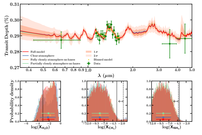
Figure 1: Atmospheric retrieval from the transmission spectrum of K2-18b. Top: Observations (green) and retrieved model spectra for the four different model considerations in Table  1. Shaded regions represent 1$\sigma$ and 2$\sigma$ confidence intervals for the full model, with yellow points showing the model binned to the data resolution. The observations were adopted from Benneke et al. (2019). Bottom: Posterior distributions for the retrieved volume mixing ratios of H₂O, CH₄, and NH₃. The 99% upper limits for the full model on CH₄ and NH₃ are shown by the arrows and dashed lines. Equilibrium solar values are shown by solid black lines.

Recent exoplanet detection surveys have revealed high occurrence rates of low-mass planets orbiting M Dwarfs (Dressing & Charbonneau, 2015; Mulders et al., 2015). The low masses, sizes and temperatures of M Dwarfs also mean that the planet-star contrast is favourable for planetary detection and characterisation. This ‘small-star opportunity’ has led to several detections of low-mass planets ($<10M_{\oplus}$) in the habitable-zones of M Dwarf hosts such as Trappist-1 (Gillon et al., 2017), Proxima Centauri (Anglada-Escudé et al., 2016), K2-18 (Montet et al., 2015; Foreman-Mackey et al., 2015), and LHS 1140 (Dittmann et al., 2017).

The habitable-zone transiting exoplanet K2-18b is a particularly good example (Foreman-Mackey et al., 2015; Montet et al., 2015). The close proximity and small size of its host star make precise measurements of the planetary mass, radius, and atmospheric spectra viable (Benneke et al., 2017; Cloutier et al., 2019), as exemplified by the recent detection of H₂O in its atmosphere (Tsiaras et al., 2019; Benneke et al., 2019). The habitable-zone temperature of K2-18b provides further impetus for detailed characterisation of its interior and atmosphere.

Given its mass ($M_{p}$ = 8.63 $\pm$ 1.35 $M_{\oplus}$, Cloutier et al. 2019) and radius ($R_{p}$ = 2.610 $\pm$ 0.087 $R_{\oplus}$, Benneke et al. 2019), K2-18b has a bulk density (2.67${}^{+0.52}_{-0.47}$ g/cm³, Benneke et al. 2019). This density, between that of Earth and Neptune, may be thought to preclude a purely rocky or icy interior and require a hydrogen-rich outer envelope. However, the extent of such an envelope and the conditions at the interface between the envelope and the underlying interior have not been explored. We note that the mass and radius of the planet have recently been revised (Benneke et al., 2019), which may have impacted inferences made using previous values (Cloutier et al., 2017; Tsiaras et al., 2019).

Previous studies of planets with similar masses and radii, such as GJ 1214b, suggested envelope mass fractions $\lesssim$7% (Rogers & Seager, 2010; Nettelmann et al., 2011; Valencia et al., 2013). GJ 1214b is expected to host super-critical H₂O below the envelope at pressures and temperatures too high to be conducive for life (Rogers & Seager, 2010). However, while GJ 1214b has an equilibrium temperature ($T_{eq}$) of $\sim 500$ K, K2-18b may be more favourable given its lower $T_{eq}\sim 250-300$ K.

In the present work, we conduct a systematic study to constrain both the atmospheric and interior composition of K2-18b based on extant data along with detailed atmospheric retrievals and internal structure models.

Table 1: Retrieved atmospheric properties from the transmission spectrum of K2-18b.

Model	$\log$(X${}_{\text{H}_{2}\text{O}}$)	$\log$(X${}_{\text{CH}_{4}}$)	$\log$(X${}_{\text{NH}_{3}}$)	$\ln$($\mathcal{Z}$)	Detection Significance (DS)
Case 1: Full model, inhomogenous clouds and hazes	$-2.11^{+1.06}_{-1.19}$	$-8.20^{+2.53}_{-2.34}$	$-8.64^{+2.15}_{-2.06}$	$179.15$	Reference
No H2O	N/A	$-1.11^{+0.53}_{-1.22}$	$-7.27^{+2.91}_{-2.92}$	$175.30$	$3.25$
Case 2: Clear atmosphere	$-2.18^{+1.35}_{-1.44}$	$-8.27^{+2.59}_{-2.42}$	$-8.60^{+2.19}_{-2.16}$	$179.05$	$1.20$
Case 3: Opaque cloud deck	$-1.80^{+0.81}_{-1.22}$	$-8.13^{+2.64}_{-2.41}$	$-8.57^{+2.30}_{-2.17}$	$179.09$	$1.06$
Case 4: Inhomogenous clouds	$-2.10^{+1.07}_{-1.28}$	$-8.26^{+2.56}_{-2.34}$	$-8.61^{+2.18}_{-2.10}$	$179.41$	N/A

Note. — Four models are considered with different treatments of clouds and hazes. For each model, the volume mixing ratios ($\log$(X${}_{\text{H}_{2}\text{O}}$), $\log$(X${}_{\text{CH}_{4}}$), and $\log$(X${}_{\text{NH}_{3}}$)) are shown along with the Bayesian evidence ($\ln$($\mathcal{Z}$)) and detection significance (DS). The DS is derived from the Bayesian evidence and a value below 2.0$\sigma$ is considered weak (Trotta, 2008). The preference of the reference model (case 1) over other models is quantified by the DS. For example, the DS for case 2 implies that case 1 is preferred over case 2 at 1.2$\sigma$. H₂O is detected at 3.25$\sigma$ and clouds/hazes at only $\sim$1$\sigma$.

2 Atmospheric Properties

We retrieve the atmospheric properties of K2-18b using its broadband transmission spectrum reported by Benneke et al. (2019). The data include observations from the HST WFC3 G141 grism (1.1-1.7 $\mu$m), photometry in the Spitzer IRAC 3.6 $\mu$m and 4.5 $\mu$m bands, and optical photometry in the K2 band (0.4-1.0 $\mu$m). We perform the atmospheric retrieval using an adaptation of the AURA retrieval code (Pinhas et al., 2019; Welbanks & Madhusudhan, 2019). Our model solves line-by-line radiative transfer in a plane-parallel atmosphere in transmission geometry. The model assumes hydrostatic equilibrium and considers prominent opacity sources in the observed spectral bands as well as homogeneous/inhomogeneous cloud/haze coverage. Clouds are included through a gray cloud deck with cloud-top pressure ($\text{P}_{\text{c}}$) as a free parameter. Hazes are included as a modification to Rayleigh-scattering through parameters for the scattering slope ($\gamma$) and a Rayleigh-enhancement factor ($a$). The opacity sources include H₂O (Rothman et al., 2010), CH₄ (Yurchenko & Tennyson, 2014), NH₃ (Yurchenko et al., 2011), CO₂ (Rothman et al., 2010), HCN (Barber et al., 2014), and collision-induced absorption due to H₂-H₂ and H₂-He (Richard et al., 2012).

The model comprises 16 free parameters: abundances of 5 molecules, 6 parameters for the pressure-temperature ($P$-$T$) profile, 4 cloud/haze parameters, and 1 parameter for the reference pressure $P_{\text{ref}}$ at $R_{p}$ (e.g., Welbanks et al., 2019). The Bayesian parameter estimation is conducted using the Nested Sampling algorithm MultiNest (Feroz et al., 2009) through PyMultiNest (Buchner et al., 2014). We conduct retrievals for four model configurations: (1) a full model including inhomogeneous clouds and hazes, (2) a clear atmosphere, (3) an atmosphere with an opaque cloud deck but no hazes, and (4) an atmosphere with inhomogeneous clouds but no hazes. The atmospheric constraints are shown in Figure 1 and Table  1.

We confirm the high-confidence detection of H₂O in a H₂-rich atmosphere as reported by Benneke et al. (2019) and Tsiaras et al. (2019). Our abundance estimates are consistent to within 1$\sigma$ between all four model configurations and with Benneke et al. (2019). The derived H₂O volume mixing ratio ranges between 0.02-14.80%, with median values of 0.7-1.6% between the 4 model cases, as shown in Table 1. The case with an opaque cloud deck (a clear atmosphere) retrieves slightly higher (lower) H₂O abundances as expected (Welbanks & Madhusudhan, 2019). Our derived H₂O abundance range corresponds to an O/H ratio of 0.2-176.8$\times$solar, assuming all the oxygen is in H₂O as expected in H₂-rich atmospheres at such low temperatures (Burrows & Sharp, 1999). The median H₂O abundance is 9.3$\times$solar for the full model, case 1. We cannot compare our results with Tsiaras et al. (2019) as their retrievals were based on only the HST WFC3 data and used older measurements of the planetary mass and radius which could have biased their inferences.

We find a depletion of CH₄ and NH₃ in the atmosphere. For a H₂-rich atmosphere at $\sim$300 K, CH₄ and NH₃ are expected to be dominant carriers of carbon and nitrogen, respectively, in chemical equilibrium (Burrows & Sharp, 1999), as also seen for the gas and ice giants in the solar system (Atreya et al., 2018). Assuming solar elemental ratios (i.e., C/O = 0.55, N/O = 0.14), the CH₄/H₂O (NH₃/H₂O) ratio is expected to be $\sim$0.5 ($\sim$0.1). However, we do not detect CH₄ or NH₃ despite their strong absorption in the HST WFC3 and/or Spitzer 3.6 $\mu$m bands. As shown in Figure 1, the retrieved posteriors of the CH₄ and NH₃ abundances are largely sub-solar, with 99% upper limits of 3.47$\times 10^{-2}$ and 5.75$\times 10^{-5}$, respectively. These sub-solar values are in contrast to the largely super-solar H₂O, arguing against chemical equilibrium at solar elemental ratios.

We do not find strong evidence for clouds/hazes in the atmosphere. Our model preference for clouds/hazes, relative to the cloud-free case, is marginal (1.2$\sigma$) compared to Benneke et al. (2019) (2.6$\sigma$). Our retrieved cloud-top pressure ($P_{c}$) for the full case is weakly constrained to 0.1 mbar to 2 bar, close to the observable photosphere. Finally, we retrieve $P_{\text{ref}}$ for the full case to be $12-174$ mbar corresponding to $R_{p}$. The median value of 0.05 bar is used as the surface boundary condition, pressure $P_{0}$, for the internal structure models in section 3.1.

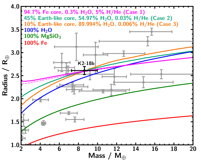
Figure 2: Model mass-radius (M-R) relations for planets with different compositions. The mass fractions are shown in the legend. The solid magenta, teal, and orange curves show cases with three representative compositions, discussed in section 4.1, that all fit the mass and radius of K2-18b equally well. The dashed magenta line represents the same composition as the solid magenta line, but with a mixed H₂O-H/He envelope. Also shown are exoplanets whose masses and radii are known to $\geq 3\sigma$ with $T_{eq}<$ 1000 K, from TEPCat (Southworth, 2011).

$\begin{array}[]{cc}\includegraphics[width=216.81pt]{k2_ternary.pdf}\includegraphics[width=216.81pt]{core_gas.pdf}\end{array}$

Figure 3: Left: Ternary diagram showing best-fitting ($\leq 1\sigma$) interior compositions allowed by the mass and radius of K2-18b for two end-member core compositions and interior temperatures. Right: Envelope vs core mass fraction for model solutions. The dark red and blue shaded regions show the same cases as in the ternary diagram. The pale blue region shows an additional case with $T_{\rm int}=25K$ and an Earth-like core for comparison. The black lines in each case show the loci of the best-fit solutions. The magenta square, teal triangle and orange circle represent the rocky world, intermediate and water world scenarios discussed in section 4. The H/He mass fraction ($x_{\rm env}$) is constrained to be $<$3.3% ($<$6.2%) for models with an Earth-like (33% Fe) core and a pure (100%) Fe core, respectively.

3 Internal Structure and Composition

In this section we use the observed bulk properties of K2-18b, namely the planetary mass ($M_{p}$), radius ($R_{p}$), and its atmospheric properties, to constrain its internal structure and thermodynamic conditions.

3.1 Internal structure model

We model the interior of the planet with a canonical four-layer structure. The model comprises a two-component Fe+rock core consisting of an inner Fe layer and an outer silicate layer, a layer of H₂O, and an outer H/He envelope. Such a model spans the possible internal structures and compositions of super-Earths and mini-Neptunes (e.g. Valencia et al., 2010, 2013; Rogers et al., 2011; Lopez & Fortney, 2014), as well as terrestrial planets and ice giants in the solar system (Guillot & Gautier, 2015). The mass fractions of the different components ($x_{\rm Fe}$, $x_{\rm rock}$, $x_{\rm H_{2}O}$, $x_{\rm env}$) are free parameters in the model and sum to unity. Our present model is adapted from a three-layer model for super-Earths from Madhusudhan et al. (2012) comprising of Fe, rock, and H₂O, with the H/He envelope added in the present work.

The model solves the standard internal structure equations of hydrostatic equilibrium and mass continuity assuming spherical symmetry. The equation of state (EOS) for each of the two inner layers is adopted from Seager et al. (2007) who use the Birch-Murnaghan EOS (Birch, 1952) for Fe (Ahrens, 1995) and MgSiO₃ perovskite (Karki et al., 2000). For the H₂O layer we use the temperature-dependent H₂O EOS compiled by Thomas & Madhusudhan (2016) from French et al. (2009); Sugimura et al. (2010); Fei et al. (1993); Seager et al. (2007) and Wagner & Pruß (2002). For the gaseous envelope we use the latest H/He EOS from Chabrier et al. (2019) for a solar helium mass fraction ($Y=0.275$).

The EOS in the H/He and H₂O layers can have a significant temperature dependence which we consider in our model. Past studies (Rogers et al., 2011; Valencia et al., 2013) considered analytic $P$-$T$ profiles for irradiated atmospheres derived using double gray approximations (Hansen, 2008; Guillot, 2010) with the internal and external fluxes and opacities as free parameters. We calculate self-consistent dayside $P$-$T$ profiles for K2-18b in the H/He envelope using the GENESIS code (Gandhi & Madhusudhan, 2017). GENESIS solves line-by-line radiative transfer under assumptions of hydrostatic, radiative-convective and thermochemical equilibrium. We include opacity due to H₂O (Rothman et al., 2010), as detected in the transmission spectrum (section 2), H₂ Rayleigh scattering, clouds and H₂-H₂ and H₂-He collision-induced absorption. We use a H₂O abundance of 10$\times$solar (see section 2) and also use 10$\times$solar abundances for the cloud species. We include KCl, ZnS and Na₂S clouds (Morley et al., 2013), for which we obtain opacities from Pinhas & Madhusudhan (2017). We further include water ice clouds using opacities from Budaj et al. (2015).

The $P$-$T$ profile also depends on the planetary internal flux, which is characterised by the internal temperature $T_{\mathrm{int}}$. We consider values of $T_{\mathrm{int}}$ which span the range expected for a planet with the mass and radius of K2-18b and an age of $1-10$ Gyr, with envelope compositions from solar to water-rich. We choose end-member cases of $T_{\mathrm{int}}=25\text{K}$ and $50\text{K}$, consistent with previous studies on planets of similar mass and radius, e.g., GJ 1214b (e.g., Valencia et al., 2013). The GENESIS models are calculated between pressures of $10^{-5}-10^{3}$ bar, and assume full redistribution of the incident stellar irradiation. We explore a range of $P$-$T$ profiles and choose two representative cases, with different $T_{\mathrm{int}}$, discussed further in sections 3.2 and 3.3. Where required by the internal structure model, the bottom of the $P$-$T$ profile of the H/He envelope is continued to deeper pressures using the adiabatic gradient from Chabrier et al. (2019). We also employ an adiabatic temperature profile in the H₂O layer, following Thomas & Madhusudhan (2016).

3.2 Constraints on interior composition

Figure 2 shows mass-radius relations for models with different interior compositions. We explore the full range of plausible interior compositions in three components: $x_{\rm core}=x_{\rm Fe}+x_{\rm rock}$, $x_{\rm H_{2}O}$, and $x_{\rm env}$, where $x_{i}$ = $M_{i}/M_{p}$ is the mass fraction of each component $i$. For each atmospheric $P$-$T$ profile considered, we explore two different core compositions: (1) an Earth-like core made of 33% Fe, 67% rock by mass, and (2) a pure Fe core, the densest possible composition. Here, we discuss results from two end-member cases: (1) a pure Fe core with $T_{\rm int}=25$K, and (2) an Earth-like (33% Fe) core with $T_{\rm int}=50$K. Solutions for all other cases lie between these two cases.

As shown in Figure 3, while a wide range of core and H₂O mass fractions are permitted, we place a stringent upper limit on the mass fraction of the H/He envelope: $x_{\rm env}=6.2$%. This maximal $x_{\rm env}$ corresponds to the case of a pure Fe core, with $x_{\rm core}\sim 94$%, underlying the H/He envelope with no $x_{\rm H_{2}O}$; here it is assumed that the atmospheric H₂O is not mixed in the envelope. However, if the retrieved atmospheric H₂O abundance is assumed to be well mixed in the envelope then the maximal $x_{\rm env}=6$% with $x_{\rm H_{2}O}=0.4$% by mass; low, but still significantly higher than that of the Earth’s oceans ($\sim$0.02%).

We find that a substantial gaseous H/He envelope is not necessary to explain the density of K2-18b. Figure 3 shows the $x_{\rm env}$ required for different $x_{\rm core}$. At one extreme, a $\sim$100% H₂O interior with no rocky core can explain the data with an $x_{\rm env}$ of just $\sim$10^-6, comparable to the mass fraction of the Earth’s atmosphere. The presence of a rocky core would necessitate at least a thin H/He envelope. However, even considering a reasonable $x_{\rm core}=10-50$% still requires $x_{\rm env}$ of only $\sim 10^{-5}-10^{-2}$, as shown in Figure 3. Model solutions with the hotter $P$-$T$ profile and/or lower Fe content in the core require smaller $x_{\rm env}$ for a given $x_{\rm core}$.

We have also considered models with miscible H₂O and H/He envelopes. We follow the approach of Soubiran & Militzer (2015), using an additive volume law for mixtures. Assuming that the median H₂O mixing ratio in the atmosphere is representative of the mixed (H₂O-H/He) envelope, we find that the difference in radius between the mixed and non-mixed models is less than half of the measured uncertainty (see Figure 2). The constraint on the envelope mass fraction from this mixed case is $x_{\rm env}=2.5-6.4$%, consistent with, and a subset of, the constraints discussed above. Note that in this case $x_{\rm env}$ includes both the H/He and H₂O mass fraction.

$\begin{array}[]{cc}\includegraphics[width=216.81pt]{profile.pdf}\includegraphics[width=216.81pt]{phase_diagram.pdf}\end{array}$

Figure 4: Left: Pressure-density profiles for three possible compositions of K2-18b discussed in Section 4. The transitions between components are marked. Right: Thermodynamic conditions at the H₂O-H/He boundary (HHB). The red lines indicate the range of possible pressures and temperatures at the HHB for two values of $T_{\rm int}$ considered. They trace the two model $P$-$T$ profiles in the H/He layer. For each case the models span both Earth-like and Fe-only core compositions. The phase diagram of H₂O is shown in the background. The square, circle and triangle correspond to the representative cases from the left-hand panel with the same color. We only show solutions with reasonable core mass fractions ($\geq$10%); less massive cores lead to lower $P$ and $T$ at the HHB. The blue lines show the adiabatic temperature profiles in the H₂O layer below the HHB for the three examples.

3.3 Atmosphere-Ocean Boundary

Our constraints on the interior compositions of K2-18b result in a wide range of thermodynamic conditions at the H₂O-H/He boundary (HHB). The pressure ($P_{\rm HHB}$) and Temperature ($T_{\rm HHB}$) at the HHB for the model solutions are shown in Figure 4. Each point on the HBB loci denotes the transition from the $P$-$T$ profile in the H/He envelope to the corresponding H₂O adiabat. The $P_{\rm HHB}$ and $T_{\rm HHB}$ depend on the H/He envelope mass fraction. For a given $P$-$T$ profile, larger envelopes result in higher $P_{\rm HHB}$ and $T_{\rm HHB}$. For example, solutions with $x_{\rm env}\gtrsim 1$% lead to $P_{\rm HHB}$ and $T_{\rm HHB}$ corresponding to the super-critical phase of H₂O. As shown in Figure 3, solutions with higher $x_{\rm env}$ correspond to higher $x_{\rm core}$ and lower $x_{\rm H_{2}O}$.

Conversely, solutions with lower $x_{\rm core}$, and hence lower $x_{\rm env}$ and higher $x_{\rm H_{2}O}$, lead to lower $P_{\rm HHB}$ and $T_{\rm HHB}$ with H₂O in vapour or liquid phases at the HHB. For example, an $x_{\rm core}\lesssim$ 30% leads to a $P_{\rm HHB}$ and $T_{\rm HHB}$ corresponding to the liquid phase of H₂O, for the cooler $P$-$T$ profile (with $T_{\rm int}=25$K). For $x_{\rm core}\sim$10% or less, the $P_{\rm HHB}$ and $T_{\rm HHB}$ approach STP conditions for liquid H₂O. Below the HHB, H₂O is found in increasingly dense phases spanning liquid, vapour, super-critical, and ice states depending on the location of the HHB and the extent of the H₂O layer, as shown in Figure 4. In the case of a mixed H₂O-H/He envelope, the HHB is undefined as it corresponds to an extreme case with no pure H₂O layer.

4 Discussion

Our constraints on the interior and atmospheric properties of K2-18b provide insights into its physical conditions, origins, and potential habitability.

4.1 Possible Compositions and Origins

Here we discuss three representative classes that span the range of possible compositions, as indicated in Figures 2, 3 and 4. The specific cases chosen here fit the $M_{\rm p}$ and $R_{\rm p}$ exactly, as shown in figure 2. A wider range of solutions exist in each of these classes within the 1$\sigma$ uncertainties.

Case 1: Rocky World. One possible scenario is a massive rocky interior overlaid by a H/He envelope. For example, a pure Fe core of 94.7% by mass with an almost maximal H/He envelope of 5% explains the data with minimal $x_{\rm H_{2}O}=0.3\%$, consistent with our retrieved H₂O abundance in the atmosphere. The HHB in this case is at $\sim 10^{6}$ bar, yielding supercritical H₂O close to the ice X phase. It is also possible in this case that the H₂O and H/He are mixed, meaning the HHB is not well-defined. Such a scenario is consistent with either H₂ outgassing from the interior (Elkins-Tanton & Seager, 2008; Rogers & Seager, 2010) or accretion of an H₂-rich envelope during formation (Lee & Chiang, 2016).

Case 2: Mini-Neptune. There are a range of plausible compositions consisting of a non-negligible H/He envelope in addition to significant H₂O and core mass fractions, akin to canonical models for Neptune and Uranus (Guillot & Gautier, 2015). One such example is a 45% Earth-like core with $x_{\rm env}=0.03\%$ and $x_{\rm H_{2}O}=54.97\%$. In this case the HHB is at $P_{\rm HHB}=700$bar and $T_{\rm HHB}=1500$K, with H₂O in the supercritical phase.

Case 3: Water World. A $\sim$100% water world with a minimal H₂-rich atmosphere ($x_{\rm env}\sim 10^{-6}$) is permissible by the data. However, such an extreme case is implausible from a planet formation perspective; some amount of rocky core is required to initiate further ice and gas accretion (Léger et al., 2004; Rogers et al., 2011; Lee & Chiang, 2016). For example, a planet with $x_{\rm core}=10\%,x_{\rm H_{2}O}=89.994\%$ and a thin H/He envelope ($x_{\rm env}=0.006\%$) can explain the data. For this case, $P_{\rm HHB}=130$bar and $T_{\rm HHB}=560$K, corresponding to liquid H₂O. For the same core fraction, solutions with even smaller H/He envelopes are admissible within the 1$\sigma$ uncertainties on $M_{p}$ and $R_{p}$, leading to $P_{\rm HHB}$ and $T_{\rm HHB}$ approaching habitable STP conditions.

4.2 Potential Habitability

A notional definition of habitability argues for a planetary surface with temperatures and pressures conducive to liquid H₂O (e.g., Kasting et al., 1993; Meadows & Barnes, 2018). Living organisms are known to thrive in Earth’s extreme environments (extremophiles). Their living conditions span the phase space of liquid H₂O up to $\sim$1000 bar pressures at the bottom of the Marianas Trench and $\sim$400 K temperatures near hydrothermal vents (e.g., Merino et al., 2019).

Whether or not habitable conditions prevail on K2-18b depends on the extent of the H/He envelope. The thermodynamic conditions at the surface of the H₂O layer span a wide range in the H₂O phase diagram. While most of these solutions lie in the super-critical phase, many others lie in the liquid and vapour phases. Model solutions with core mass fractions $<$15% and H/He envelopes $\lesssim 10^{-3}$ allow for liquid H₂O at Earth-like habitable conditions discussed above. One plausible scenario is an ocean world, as discussed in section 4.1, with liquid water approaching STP conditions (e.g., 300 K, $\sim$1-10 bar) underneath a thin H/He atmosphere ($x_{\rm env}\lesssim$10^-5).

A number of studies in the past have argued for potential habitability on planets with H/He-rich atmospheres orbiting M Dwarfs (e.g., Pierrehumbert & Gaidos, 2011; Seager et al., 2013; Koll & Cronin, 2019). Given our constraints above, we find that K2-18b has a realistic chance of being habitable. Furthermore, our constraints on CH₄ and NH₃ suggest chemical disequilibrium. Among other possibilities for chemical disequilibrium, e.g. photochemistry, the potential influence of biochemical processes may not be entirely ruled out. Future observations, e.g. with the James Webb Space Telescope, will have the potential to refine our findings. We argue that planets such as K2-18b can indeed have the potential to approach habitable conditions and searches for biosignatures should not necessarily be restricted to smaller rocky planets.

References

- Ahrens (1995) Ahrens, T. J., ed. 1995, Mineral Physics & Crystallography: A Handbook of Physical Constants (American Geophysical Union), doi: 10.1029/rf002
- Anglada-Escudé et al. (2016) Anglada-Escudé, G., Amado, P. J., Barnes, J., et al. 2016, Nature, 536, 437, doi: 10.1038/nature19106
- Atreya et al. (2018) Atreya, S. K., Crida, A., Guillot, T., et al. 2018, The Origin and Evolution of Saturn, with Exoplanet Perspective in, Saturn in the 21st Century, ed. K. H. Baines et al. (Cambridge: Cambridge Univ. Press), 5–43, doi: 10.1017/9781316227220.002
- Barber et al. (2014) Barber, R. J., Strange, J. K., Hill, C., et al. 2014, MNRAS, 437, 1828, doi: 10.1093/mnras/stt2011
- Benneke et al. (2017) Benneke, B., Werner, M., Petigura, E., et al. 2017, ApJ, 834, 187, doi: 10.3847/1538-4357/834/2/187
- Benneke et al. (2019) Benneke, B., Wong, I., Piaulet, C., et al. 2019, ApJ, 887, L14, doi: 10.3847/2041-8213/ab59dc
- Birch (1952) Birch, F. 1952, J. Geophys. Res., 57, 227, doi: 10.1029/JZ057i002p00227
- Buchner et al. (2014) Buchner, J., Georgakakis, A., Nandra, K., et al. 2014, A&A, 564, A125, doi: 10.1051/0004-6361/201322971
- Budaj et al. (2015) Budaj, J., Kocifaj, M., Salmeron, R., & Hubeny, I. 2015, MNRAS, 454, 2, doi: 10.1093/mnras/stv1711
- Burrows & Sharp (1999) Burrows, A., & Sharp, C. M. 1999, ApJ, 512, 843, doi: 10.1086/306811
- Chabrier et al. (2019) Chabrier, G., Mazevet, S., & Soubiran, F. 2019, ApJ, 872, 51, doi: 10.3847/1538-4357/aaf99f
- Cloutier et al. (2017) Cloutier, R., Astudillo-Defru, N., Doyon, R., et al. 2017, A&A, 608, A35, doi: 10.1051/0004-6361/201731558
- Cloutier et al. (2019) —. 2019, A&A, 621, A49, doi: 10.1051/0004-6361/201833995
- Dittmann et al. (2017) Dittmann, J. A., Irwin, J. M., Charbonneau, D., et al. 2017, Nature, 544, 333, doi: 10.1038/nature22055
- Dressing & Charbonneau (2015) Dressing, C. D., & Charbonneau, D. 2015, ApJ, 807, 45, doi: 10.1088/0004-637X/807/1/45
- Elkins-Tanton & Seager (2008) Elkins-Tanton, L. T., & Seager, S. 2008, ApJ, 685, 1237, doi: 10.1086/591433
- Fei et al. (1993) Fei, Y., Mao, H., & Hemley, R. J. 1993, The Journal of Chemical Physics, 99, 5369, doi: 10.1063/1.465980
- Feroz et al. (2009) Feroz, F., Hobson, M. P., & Bridges, M. 2009, MNRAS, 398, 1601, doi: 10.1111/j.1365-2966.2009.14548.x
- Foreman-Mackey et al. (2015) Foreman-Mackey, D., Montet, B. T., Hogg, D. W., et al. 2015, ApJ, 806, 215, doi: 10.1088/0004-637X/806/2/215
- French et al. (2009) French, M., Mattsson, T. R., Nettelmann, N., & Redmer, R. 2009, Phys. Rev. B, 79, 054107, doi: 10.1103/PhysRevB.79.054107
- Gandhi & Madhusudhan (2017) Gandhi, S., & Madhusudhan, N. 2017, MNRAS, 472, 2334, doi: 10.1093/mnras/stx1601
- Gillon et al. (2017) Gillon, M., Triaud, A. H. M. J., Demory, B.-O., et al. 2017, Nature, 542, 456, doi: 10.1038/nature21360
- Guillot (2010) Guillot, T. 2010, A&A, 520, A27, doi: 10.1051/0004-6361/200913396
- Guillot & Gautier (2015) Guillot, T., & Gautier, D. 2015, in Treatise on Geophysics, 2nd edn., ed. G. Schubert (Oxford: Elsevier), 529 – 557, doi: https://doi.org/10.1016/B978-0-444-53802-4.00176-7
- Hansen (2008) Hansen, B. M. S. 2008, ApJS, 179, 484, doi: 10.1086/591964
- Karki et al. (2000) Karki, B. B., Wentzcovitch, R. M., de Gironcoli, S., & Baroni, S. 2000, Phys. Rev. B, 62, 14750, doi: 10.1103/PhysRevB.62.14750
- Kasting et al. (1993) Kasting, J. F., Whitmire, D. P., & Reynolds, R. T. 1993, Icarus, 101, 108, doi: 10.1006/icar.1993.1010
- Koll & Cronin (2019) Koll, D. D. B., & Cronin, T. W. 2019, ApJ, 881, 120, doi: 10.3847/1538-4357/ab30c4
- Lee & Chiang (2016) Lee, E. J., & Chiang, E. 2016, ApJ, 817, 90, doi: 10.3847/0004-637X/817/2/90
- Léger et al. (2004) Léger, A., Selsis, F., Sotin, C., et al. 2004, Icarus, 169, 499, doi: 10.1016/j.icarus.2004.01.001
- Lopez & Fortney (2014) Lopez, E. D., & Fortney, J. J. 2014, ApJ, 792, 1, doi: 10.1088/0004-637X/792/1/1
- Madhusudhan et al. (2012) Madhusudhan, N., Lee, K. K. M., & Mousis, O. 2012, ApJ, 759, L40, doi: 10.1088/2041-8205/759/2/L40
- Meadows & Barnes (2018) Meadows, V. S., & Barnes, R. K. 2018, Factors Affecting Exoplanet Habitability (Springer International Publishing), 57, doi: 10.1007/978-3-319-55333-7_57
- Merino et al. (2019) Merino, N., Aronson, H. S., Bojanova, D. P., et al. 2019, Frontiers in Microbiology, 10, 780, doi: 10.3389/fmicb.2019.00780
- Montet et al. (2015) Montet, B. T., Morton, T. D., Foreman-Mackey, D., et al. 2015, ApJ, 809, 25, doi: 10.1088/0004-637X/809/1/25
- Morley et al. (2013) Morley, C. V., Fortney, J. J., Kempton, E. M. R., et al. 2013, ApJ, 775, 33, doi: 10.1088/0004-637X/775/1/33
- Mulders et al. (2015) Mulders, G. D., Pascucci, I., & Apai, D. 2015, ApJ, 814, 130, doi: 10.1088/0004-637X/814/2/130
- Nettelmann et al. (2011) Nettelmann, N., Fortney, J. J., Kramm, U., & Redmer, R. 2011, ApJ, 733, 2, doi: 10.1088/0004-637X/733/1/2
- Pierrehumbert & Gaidos (2011) Pierrehumbert, R., & Gaidos, E. 2011, ApJ, 734, L13, doi: 10.1088/2041-8205/734/1/L13
- Pinhas & Madhusudhan (2017) Pinhas, A., & Madhusudhan, N. 2017, MNRAS, 471, 4355, doi: 10.1093/mnras/stx1849
- Pinhas et al. (2019) Pinhas, A., Madhusudhan, N., Gandhi, S., & MacDonald, R. 2019, MNRAS, 482, 1485, doi: 10.1093/mnras/sty2544
- Richard et al. (2012) Richard, C., Gordon, I. E., Rothman, L. S., et al. 2012, J. Quant. Spec. Radiat. Transf., 113, 1276, doi: 10.1016/j.jqsrt.2011.11.004
- Rogers et al. (2011) Rogers, L. A., Bodenheimer, P., Lissauer, J. J., & Seager, S. 2011, ApJ, 738, 59, doi: 10.1088/0004-637X/738/1/59
- Rogers & Seager (2010) Rogers, L. A., & Seager, S. 2010, ApJ, 716, 1208, doi: 10.1088/0004-637X/716/2/1208
- Rothman et al. (2010) Rothman, L. S., Gordon, I. E., Barber, R. J., et al. 2010, J. Quant. Spec. Radiat. Transf., 111, 2139, doi: 10.1016/j.jqsrt.2010.05.001
- Seager et al. (2013) Seager, S., Bains, W., & Hu, R. 2013, ApJ, 777, 95, doi: 10.1088/0004-637X/777/2/95
- Seager et al. (2007) Seager, S., Kuchner, M., Hier-Majumder, C. A., & Militzer, B. 2007, ApJ, 669, 1279, doi: 10.1086/521346
- Soubiran & Militzer (2015) Soubiran, F., & Militzer, B. 2015, ApJ, 806, 228, doi: 10.1088/0004-637X/806/2/228
- Southworth (2011) Southworth, J. 2011, MNRAS, 417, 2166, doi: 10.1111/j.1365-2966.2011.19399.x
- Sugimura et al. (2010) Sugimura, E., Komabayashi, T., Hirose, K., et al. 2010, Phys. Rev. B, 82, 134103, doi: 10.1103/PhysRevB.82.134103
- Thomas & Madhusudhan (2016) Thomas, S. W., & Madhusudhan, N. 2016, MNRAS, 458, 1330, doi: 10.1093/mnras/stw321
- Trotta (2008) Trotta, R. 2008, Contemporary Physics, 49, 71, doi: 10.1080/00107510802066753
- Tsiaras et al. (2019) Tsiaras, A., Waldmann, I. P., Tinetti, G., Tennyson, J., & Yurchenko, S. N. 2019, NatAs, 3, 1086, doi: 10.1038/s41550-019-0878-9
- Valencia et al. (2013) Valencia, D., Guillot, T., Parmentier, V., & Freedman, R. S. 2013, ApJ, 775, 10, doi: 10.1088/0004-637X/775/1/10
- Valencia et al. (2010) Valencia, D., Ikoma, M., Guillot, T., & Nettelmann, N. 2010, A&A, 516, A20, doi: 10.1051/0004-6361/200912839
- Wagner & Pruß (2002) Wagner, W., & Pruß, A. 2002, Journal of Physical and Chemical Reference Data, 31, 387, doi: 10.1063/1.1461829
- Welbanks & Madhusudhan (2019) Welbanks, L., & Madhusudhan, N. 2019, AJ, 157, 206, doi: 10.3847/1538-3881/ab14de
- Welbanks et al. (2019) Welbanks, L., Madhusudhan, N., Allard, N. F., et al. 2019, ApJ, 887, L20, doi: 10.3847/2041-8213/ab5a89
- Yurchenko et al. (2011) Yurchenko, S. N., Barber, R. J., & Tennyson, J. 2011, MNRAS, 413, 1828, doi: 10.1111/j.1365-2966.2011.18261.x
- Yurchenko & Tennyson (2014) Yurchenko, S. N., & Tennyson, J. 2014, MNRAS, 440, 1649, doi: 10.1093/mnras/stu326