Parton showers beyond leading logarithmic accuracy

Abstract

Parton showers are among the most widely used tools in collider physics. Despite their key importance, none so far has been able to demonstrate accuracy beyond a basic level known as leading logarithmic (LL) order, with ensuing limitations across a broad spectrum of physics applications. In this letter, we propose criteria for showers to be considered next-to-leading logarithmic (NLL) accurate. We then introduce new classes of shower, for final-state radiation, that satisfy the main elements of these criteria in the widely used large-$N_{C}$ limit. As a proof of concept, we demonstrate these showers’ agreement with all-order analytical NLL calculations for a range of observables, something never so far achieved for any parton shower.

High-energy particle collisions produce complex hadronic final states. Understanding these final states is of crucial importance in order to extract maximal information about the underlying energetic scattering processes and the fundamental Lagrangian of particle physics. To do so, there is ubiquitous reliance on general purpose Monte Carlo (GPMC) event generators Buckley et al. (2011), which provide realistic simulations of full events. A core component of GPMCs is the parton shower, a subject of much recent research Sjostrand and Skands (2005); Giele et al. (2008); Nagy and Soper (2007); Schumann and Krauss (2008); Platzer and Gieseke (2011); Jadach et al. (2010); Nagy and Soper (2012, 2014, 2015); Hoeche and Prestel (2015); Li and Skands (2017); Jadach et al. (2016); Fischer et al. (2016); Nagy and Soper (2016); Fischer et al. (2017); Hoeche et al. (2017); Hoeche and Prestel (2017); Nagy and Soper (2018); Cabouat and Sjöstrand (2018); Dulat et al. (2018); Plaetzer et al. (2018); Ángeles Martínez et al. (2018); Isaacson and Prestel (2019); Brooks and Skands (2019); Forshaw et al. (2019); Nagy and Soper (2019); Hoeche and Reichelt (2020). Partons refer to quarks and gluons, and a shower aims to encode the dynamics of parton production between the high-energy scattering (e.g. production of electroweak or new-physics states) and the low scale of hadronic Quantum Chromodynamics (QCD), at which experimental observations are made.

Typically parton showers are built using a simple Markovian algorithm that takes an $n$-parton state and stochastically maps it to an $n+1$-parton state. The iteration of this procedure, e.g. starting from a 2-parton state, builds up events with numerous partons. A further step, hadronisation, then maps the partons onto a set of hadrons. Even though this last step involves modelling Buckley et al. (2010); Skands (2010), many of the features of the resulting events are driven by the parton shower component which is, in principle, within the realm of calculations in perturbative QCD. This is because the showering occurs at momentum scales where the strong coupling, $\alpha_{s}$ is small.

Much of collider physics, experimental and theoretical Keith Ellis and Zanderighi (2019); Azzi et al. (2019); Cepeda et al. (2019); Cid Vidal et al. (2019), is moving towards high precision, especially in view of large volumes of data collected so far at CERN’s Large Hadron Collider (LHC). On the theoretical front many of the advances either involve approximations with a small number of partons, or else are specific to individual observables. Parton showers, in contrast, use a single algorithm to describe arbitrary observables of any complexity. This versatility comes at a cost: lesser accuracy for any specific observable and, quite generally, at best only limited knowledge Marchesini and Webber (1984); Banfi et al. (2007); Dasgupta et al. (2018); Bewick et al. (2019) of what the accuracy even is for a given observable. In fact there is currently no readily accepted criterion for categorising the accuracy of parton showers. One novel element that we introduce in this paper is therefore a set of criteria for doing so.

The role of showers is to reproduce emissions across disparate scales. Our first criterion for accuracy starts by structuring this phase space: there are three phase space variables per emission, and two of them (e.g. energy and angle) are associated with logarithmic divergences in the product of squared matrix element and phase space. We define LL accuracy to include a condition that the shower should generate the correct effective squared tree-level matrix element in a limit where every pair of emissions has distinctly different values for both logarithmic variables. At NLL accuracy, we further require that the shower generate the correct squared tree-level matrix element in a limit where every pair of emissions has distinctly different values for at least one of the logarithmic variables (or some linear combination of their logarithms). Beyond NLL accuracy we would consider configurations with a pair of emissions (or multiple pairs) both of whose logarithmic variables are similar.

To help make this discussion concrete, let us consider showers that are not NLL accurate according to this criterion: angular ordered showers Marchesini and Webber (1988); Corcella et al. (2001); Bahr et al. (2008) do not reproduce the matrix element for configurations ordered in energy, but with commensurate angles, and this is associated with their inability to correctly predict $\alpha_{s}^{n}L^{n}$ (NLL) effects for non-global observables Banfi et al. (2007). Transverse-momentum ($k_{t}$) ordered showers with dipole-local recoil Gustafson and Pettersson (1988); Lonnblad (1992); Sjostrand and Skands (2005); Giele et al. (2008); Schumann and Krauss (2008); Hoeche and Prestel (2015) do not reproduce matrix elements for configurations ordered in angle but with commensurate transverse momenta, because of the way they assign transverse recoil Dasgupta et al. (2018). As a result they fail to reproduce NLL effects in global observables such as jet broadenings. Showers that omit spin correlations fail to reproduce (the azimuthal structure of) matrix elements for configurations ordered in angle but with commensurate energies Webber (1986); Collins (1988); Catani and Grazzini (2011), and associated NLL terms.

Our second criterion for logarithmic accuracy tests, among other things, the overall correctness of virtual corrections. For showers that intertwine real and virtual corrections directly through unitarity, once the generation of tree-level matrix elements is set, there is only one (single-emission) degree of freedom that remains, namely the choice of scale and scheme for the strong coupling for each emission, as a function of its kinematics. To claim NLL accuracy, we will require the resulting shower to reproduce known analytical NLL resummations across recursively infrared and collinear safe (rIRC) Banfi et al. (2005) global and non-global two-scale observables as well as (subjet) multiplicities.

The challenge that we concentrate on here is to formulate showers that can handle each of two regions correctly: the energy-ordered, commensurate-angle region; and the angular-ordered, commensurate $k_{t}$ region. Recall that existing $k_{t}$ and angular-ordered showers can each handle one of these limits, but not both. Strictly, full NLL accuracy also requires attention to the angular-ordered, commensurate energy region. However, given that general solutions for the required spin correlations are known to exist Collins (1988); Knowles (1990); Nagy and Soper (2008); Richardson and Webster (2020), and that they affect only a small subset of observables, we postpone their study to future work. For now, we also restrict our attention to final-state showers (i.e. lepton-lepton collisions), massless quarks and the large-$N_{C}$ limit. Our guiding principle will be that soft emissions should not affect, or be affected by, subsequent emissions at disparate rapidities.

The two classes of shower that we develop both consider emissions from colour dipoles. We consider a continuous family of shower evolution variables $v$, parameterised by a quantity $\beta$ in the range $0\leq\beta<1$, where $\beta=0$ corresponds to transverse-momentum ordering. The phase space involves two further variables besides $v$: a pseudorapidity-like variable within the dipole, $\bar{\eta}$, and an azimuthal angle $\phi$.

We start with a shower with dipole-local recoil (the PanLocal shower). Its mapping for emission of momentum $p_{k}$ from a dipole $\{{\widetilde{p}}_{i},{\widetilde{p}}_{j}\}$ is

$$p_{k} =a_{k}\tilde{p}_{i}+b_{k}\tilde{p}_{j}+k_{\perp}\,,$$ (1a)

$$p_{i} =a_{i}\tilde{p}_{i}+b_{i}\tilde{p}_{j}-fk_{\perp}\,,$$ (1b)

$$p_{j} =a_{j}\tilde{p}_{i}+b_{j}\tilde{p}_{j}-(1-f)k_{\perp}\,,$$ (1c)

where $k_{\perp}=k_{t}\left[{n}_{\perp,1}\cos\phi+{n}_{\perp,2}\sin\phi\right]$, with ${n}_{\perp,m}^{2}=-1$, ${n}_{\perp,m}\cdot{\widetilde{p}}_{i/j}=0$ ($m=1,2$), ${n}_{\perp,1}\cdot{n}_{\perp,2}=0$ and

$$k_{t}=\rho ve^{\beta|\bar{\eta}|}\,,\qquad\rho=\left(\frac{s_{{\tilde{\imath}}}s_{{\tilde{\jmath}}}}{Q^{2}s_{{\tilde{\imath}}{\tilde{\jmath}}}}\right)^{\frac{\beta}{2}}\,.$$ (2)

Here $s_{{\tilde{\imath}}{\tilde{\jmath}}}=2{\widetilde{p}}_{i}\cdot{\widetilde{p}}_{j}$, $s_{{\tilde{\imath}}}=2{\widetilde{p}}_{i}\cdot Q$, and $Q$ is the total event momentum. The light-cone components of $p_{k}$ are given by

$$a_{k}\equiv\sqrt{\frac{s_{{\tilde{\jmath}}}}{s_{{\tilde{\imath}}{\tilde{\jmath}}}s_{{\tilde{\imath}}}}}\,k_{t}{e}^{+\bar{\eta}}\,,\qquad b_{k}\equiv\sqrt{\frac{s_{{\tilde{\imath}}}}{s_{{\tilde{\imath}}{\tilde{\jmath}}}s_{{\tilde{\jmath}}}}}\,k_{t}{e}^{-\bar{\eta}}\,,$$ (3)

The quantity $f$ in Eq. (1) determines how transverse recoil is shared between $p_{i}$ and $p_{j}$, cf. below. The $a_{i},b_{i},a_{j},b_{j}$ are fully specified by the requirements $p^{2}_{i/j}=0$, $(p_{i}+p_{j}+p_{k})=({\widetilde{p}}_{i}+{\widetilde{p}}_{j})$ and $p_{i}=\tilde{p}_{i}$ for $k_{t}\to 0$ and are given explicitly in Ref. Dasgupta et al. (2020)§.1.

In the event centre-of-mass frame, $\bar{\eta}=0$ corresponds to a direction equidistant in angle from ${\widetilde{p}}_{i}$ and ${\widetilde{p}}_{j}$. For soft-collinear emissions, the physical pseudorapidity, $\eta=-\ln\tan\frac{\theta}{2}$, with respect to the emitter is $\eta=|\bar{\eta}|+\frac{1}{\beta}\ln\rho$. Soft-collinear emissions from distinct dipoles but with the same $\ln v$ fall onto common contours in the Lund plane Andersson et al. (1989), $k_{t}=ve^{\beta|\eta|}$.

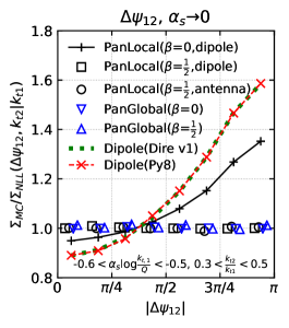
Figure 1: Left: distribution for the difference in azimuthal angle between the two highest-$k_{t}$ primary Lund declusterings in the Pythia8 dipole shower algorithm, normalised to the NLL result Banfi et al. (2002), Dasgupta et al. (2020)§.4; successively smaller $\alpha_{s}$ values keep fixed $\alpha_{s}\ln k_{t1}$. Middle: the same for the PanGlobal($\beta=0$) shower. Right: the $\alpha_{s}\to 0$ limit of the ratio for multiple showers. This observable directly tests part of our NLL (squared) matrix-element correctness condition. A unit value for the ratio signals success.

For $e^{+}e^{-}\to\text{hadrons}$, the shower starts from a 2-parton $q\bar{q}$ state, $\mathcal{S}_{2}$. The probability of evolving from $\mathcal{S}_{n}\to\mathcal{S}_{n+1}$ in a given slice $d\ln v$ of evolution variable is

$$\frac{d\mathcal{P}_{n\to n+1}}{d\ln v}=\sum_{\text{dipoles }\{{\tilde{\imath}},{\tilde{\jmath}}\}}\int d\bar{\eta}\frac{d\phi}{2\pi}\frac{\alpha_{s}(k_{t})+K\alpha_{s}^{2}(k_{t})}{\pi}\\ \times\left[g(\bar{\eta})a_{k}P_{{\tilde{\imath}}\to ik}(a_{k})+g(-\bar{\eta})b_{k}P_{{\tilde{\jmath}}\to jk}(b_{k})\right],$$ (4)

with a function $g(\bar{\eta})$ that satisfies $g(\bar{\eta})+g(-\bar{\eta})=1$, has $g(\bar{\eta})=0$ ($1$) for sufficiently negative (positive) $\bar{\eta}$, and smoothly transitions around $\bar{\eta}=0$. The $P_{{\tilde{\imath}}\to ik}(z)$ are first-order splitting functions Gribov and Lipatov (1972); Altarelli and Parisi (1977); Dokshitzer (1977), normalised so that $\lim_{z\to 0}zP_{{\tilde{\imath}}\to ik}(z)=2\,C$ with $C=C_{F}=C_{A}/2=\frac{4}{3}$ (our large-$N_{C}$ approximation, augmented Behring et al. (2019) with $n_{f}=5$). The specific choice of $g(\bar{\eta})$ is not critical here, while the splitting functions are standard. Both are detailed in Ref. Dasgupta et al. (2020)§.1. The $\overline{\text{MS}}$ coupling, $\alpha_{s}(k_{t})$, needs at least 2-loop running, and $K=\frac{1}{2\pi}\left[\left(\frac{67}{18}-\frac{\pi^{2}}{6}\right)C_{A}-\frac{5}{9}n_{f}\right]$ Catani et al. (1991a).

The PanLocal shower comes in two variants. In a dipole variant, inspired by many earlier dipole showers Schumann and Krauss (2008); Sjostrand and Skands (2005); Hoeche and Prestel (2015), the $P_{{\tilde{\imath}}\to ik}(a_{k})$ ($P_{{\tilde{\jmath}}\to jk}(b_{k})$) term of Eq. (4) is associated with the choice $f=1$ ($f=0$) in Eq. (1). In an antenna variant, inspired by Refs. Lonnblad (1992); Giele et al. (2008), we take a common $f(\bar{\eta})$ for both terms and set $f(\bar{\eta})=g(\bar{\eta})$.

A key difference relative to earlier showers is that our transition in transverse recoil assignment between $i$ and $j$ takes place at $\bar{\eta}\simeq 0$, i.e. equal angles between the ${\widetilde{p}}_{i}$ and ${\widetilde{p}}_{j}$ directions in the event centre-of-mass frame (note similarities with Deductor Nagy and Soper (2014)). This differs from the common choice of a transition in the middle of the dipole centre-of-mass frame. Our choice ensures that a given emission will not induce transverse recoil in earlier, lower-rapidity emissions. Additionally, we require $\beta>0$ in the definition of the ordering variable, Eq. (2). This causes emissions at commensurate $k_{t}$ and widely separated in $|\eta|$ to be effectively produced in order of increasing $|\eta|$, so that any significant $k_{t}$ recoil is always taken from the extremities of a (hard) $qg\{\ldots\}g\bar{q}$ dipole chain. Together, these two elements provide a solution to the problem observed in Ref. Dasgupta et al. (2018), i.e. that recoil assignment in common dipole showers causes multi-gluon emission matrix elements to be incorrect in the limit of similar $k_{t}$’s and disparate angles, starting from $\alpha_{s}^{2}$, leading to incorrect NLL terms.

Note that with dipole-local recoil, NLL correctness also requires $\beta<1$, because with $\beta\geq 1$ the kinematic constraint associated with fixed dipole mass means that a first emission cuts out regions of phase space for a second emission at similar $\ln v$.

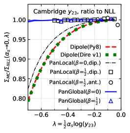
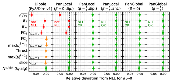
Figure 2: Left: ratio of the cumulative $y_{23}$ distribution from several showers divided by the NLL answer, as a function of $\alpha_{s}\ln y_{23}/2$, for $\alpha_{s}\to 0$. Right: summary of deviations from NLL for many shower/observable combinations (either $\Sigma_{\text{shower}}(\alpha_{s}\to 0,\alpha_{s}L=-0.5)/\Sigma_{\text{NLL}}-1$ or $(N^{\text{subjet}}_{\text{shower}}(\alpha_{s}\to 0,\alpha_{s}L^{2}=5)/N^{\text{subjet}}_{\text{NLL}}-1)/\sqrt{\alpha_{s}}$). Red squares indicate clear NLL failure; amber triangles indicate NLL fixed-order failure that is masked at all orders; green circles indicate that all NLL tests passed.

A second class of shower can be constructed with global, i.e. event-wide recoil (the PanGlobal shower). It can be formulated in largely the same terms as the dipole-local recoil shower, but with a two-step recoil procedure. In the first step one sets

$$\bar{p}_{k} =a_{k}\tilde{p}_{i}+b_{k}\tilde{p}_{j}+k_{\perp}\,,$$ (5a)

$$\bar{p}_{i} =(1-a_{k})\tilde{p}_{i}\,,$$ (5b)

$$\bar{p}_{j} =(1-b_{k})\tilde{p}_{j}\,.$$ (5c)

The second step is to apply a boost and rescaling to the full event (including the $\bar{p}_{i,j,k}$ momenta) so as to obtain final momenta $\{p\}$ whose sum gives $Q$. This approach assigns transverse recoil dominantly to the most energetic particles in the event. Thus emission from a hard $qg\{\ldots\}g\bar{q}$ dipole string transfers its recoil mostly to the hard $q$ and $\bar{q}$ ends. This ensures that one reproduces a pattern of independent emission for commensurate-$k_{t}$ and angular-ordered gluons, while also retaining the correct (dipole) pattern for energy-ordered, commensurate angles. This holds even for $\beta=0$, i.e. with $k_{t}$ ordering. Values of $\beta\geq 1$ remain problematic, however. Note that the PanGlobal shower has power-suppressed routes to highly collimated events. These compete with normal Sudakov suppression, as observed also for Pythia8 Dasgupta et al. (2018). We have verified that such effects are small even at the very edges of future (FCC-hh Abada et al. (2019)) phenomenologically accessible regions. Nevertheless, ultimately one may wish to explore alternative global recoil schemes.

The next step is to compare our showers to NLL observables. Relative to earlier attempts at such comparisons Hoeche et al. (2018), a critical novel aspect is how we isolate the structure of NLL terms $\alpha_{s}^{n}L^{n}$. For each given observable $v$, with $L=\ln v$, we consider the ratio to the true NLL result in the limit $\alpha_{s}\equiv\alpha_{s}(Q)\to 0$ with fixed $\alpha_{s}L$. This helps us isolate the NLL terms from yet higher-order contributions, which vanish in that limit. Numerically, a parton shower cannot be run in the $\alpha_{s}\to 0$ limit for fixed $\alpha_{s}L$. However, with suitable techniques Dasgupta et al. (2020)§.6, Hida et al. (2000); Lipowski and Lipowska (2011); Kleiss and Verheyen (2016), one can run multiple small values of $\alpha_{s}$ and extrapolate to $\alpha_{s}=0$. We examine not just our showers, but also our implementations of two typical $k_{t}$-ordered shower algorithms with dipole-local recoil, those of Pythia8 Sjostrand and Skands (2005) and Dire v1 Hoeche and Prestel (2015) (with the $\alpha_{s}+K\alpha_{s}^{2}$ choice as in Eq. (4)).

A first test concerns the multiple-emission matrix element. We have constructed our showers specifically so that they reproduce the squared matrix elements in the limits discussed above that are relevant for NLL accuracy. A simple observable for testing this is to consider the two highest-$k_{t}$ Lund-plane primary declusterings Dreyer et al. (2018); Andrews et al. (2018) with transverse momenta $k_{t1}$ and $k_{t2}$ (originally defined for hadronic collisions, the $e^{+}e^{-}$ analogue is given in Ref. Dasgupta et al. (2020)§.4 and implemented with FastJet Cacciari et al. (2012)). The $\alpha_{s}\to 0$ limit for fixed $\alpha_{s}L$ ($L=\ln k_{t1}/Q$), ensures that the two declusterings are soft and widely separated in Lund-plane pseudorapidity $\eta$ (which spans $|\eta|\lesssim|L|\sim 1/\alpha_{s}$). In this limit the full matrix element reduces to independent emission and so the difference of azimuthal angles between the two emissions, $\Delta\psi_{12}$, should be uniformly distributed, for any ratio $k_{t2}/k_{t1}$ (recall that strongly angular-ordered soft emission is not affected by spin correlations). We consider the $\Delta\psi_{12}$ distribution in Fig. 1.

The left-hand plot of Fig. 1 shows the Pythia8 dipole algorithm (not designed as NLL accurate), while the middle plot shows our PanGlobal shower with $\beta=0$. The dipole result is clearly not independent of $\Delta\psi_{12}$ for $\alpha_{s}\to 0$, with over $60\%$ discrepancies, extending the fixed-order conclusions of Ref. Dasgupta et al. (2018). The discrepancy is only $\simeq 30\%$ for $gg$ events (not shown in Fig. 1), and the difference would, e.g., skew machine learning Larkoski et al. (2020) for quark/gluon discrimination. PanGlobal is independent of $\Delta\psi_{12}$. The right-hand plot shows the $\alpha_{s}\to 0$ limit for multiple showers. The overall pattern is as expected: PanLocal works for $\beta=0.5$, but not $\beta=0$, demonstrating that with $k_{t}$ ordering it is not sufficient just to change the dipole partition to get NLL accuracy. PanGlobal works for $\beta=0$ and $\beta=0.5$. (Showers that coincide for $\alpha_{s}\to 0$, e.g. Dire v1 and Pythia8, typically differ at finite $\alpha_{s}$, reflecting NNLL differences.)

Next, we consider a range of more standard observables at NLL accuracy. They include the Cambridge $\sqrt{y_{23}}$ resolution scale Dokshitzer et al. (1997); two jet broadenings, $B_{T}$ and $B_{W}$ Catani et al. (1992a); fractional moments, $\text{FC}_{1-\beta_{\text{obs}}}$, of the energy-energy correlations Banfi et al. (2005); the thrust Brandt et al. (1964); Farhi (1977), and the maximum $u_{i}=k_{ti}/Qe^{-\beta_{\text{obs}}|\eta_{i}|}$ among primary Lund declusterings $i$. Each of these is sensitive to soft-collinear radiation as $k_{t}/Qe^{-\beta_{\text{obs}}|\eta|}$, with the $\beta_{\text{obs}}$ values shown in Fig. 2 (right). Additionally, the scalar sum of the transverse momenta in a rapidity slice Dasgupta and Salam (2002), of full-width $2$, is useful to test non-global logarithms (NGLs). These observables all have the property that their distribution at NLL can be written as Banfi et al. (2002); Dokshitzer et al. (1998); Banfi et al. (2005); Catani et al. (1993); Dasgupta and Salam (2002)

$$\Sigma(\alpha_{s},\alpha_{s}L)=\exp\!\left[\alpha_{s}^{\!-1}g_{1}(\alpha_{s}L)+g_{2}(\alpha_{s}L)+{\cal O}\!\left(\alpha_{s}^{n}L^{n-1}\right)\right]\!,$$ (6)

where $\Sigma$ is the fraction of events where the observable is smaller than $e^{L}$ ($g_{1}=0$ for the rapidity slice $k_{t}$). We also consider the $k_{t}$-algorithm Catani et al. (1991b) subjet multiplicity Catani et al. (1992b), Dasgupta et al. (2020)§.5.

Fig. 2 (left) illustrates our all-order tests of the shower for one observable, $\sqrt{y_{23}}$. It shows the ratio of the $\Sigma$ as calculated with the shower to the NLL result, as a function of $\alpha_{s}\ln\sqrt{y_{23}}$ in the limit of $\alpha_{s}\to 0$. The standard dipole algorithms disagree with the NLL result, by up to $20\%$. This is non-negligible, though smaller than the disagreement in Fig. 1, because of the azimuthally averaged nature of the $\sqrt{y_{23}}$ observable. In contrast the PanGlobal and PanLocal($\beta=0.5$) showers agree with the NLL result to within statistical uncertainties.

Fig. 2 (right) shows an overall summary of our tests. The position of each point shows the result of $\Sigma_{\text{shower}}(\alpha_{s}\to 0,\alpha_{s}L=-0.5)/\Sigma_{\text{NLL}}-1$ or $(N^{\text{subjet}}_{\text{shower}}(\alpha_{s}\to 0,\alpha_{s}L^{2}=5)/N^{\text{subjet}}_{\text{NLL}}-1)/\sqrt{\alpha_{s}}$. If it differs from $0$, the point is shown as a red square. In some cases (amber triangles) it agrees with $0$, though an additional fixed-order analysis in a fixed-coupling toy shower Dasgupta et al. (2018) Dasgupta et al. (2020)§.2 reveals issues affecting NLL accuracy, all involving hitherto undiscovered spurious super-leading logarithmic terms.

Green circles in Fig. 2 (right) indicate that the shower/observable combination passes all of our NLL tests, both at all orders and in fixed-order expansions. The four shower algorithms designed to be NLL accurate pass all the tests. These are the PanLocal shower (dipole and antenna variants) with $\beta=\frac{1}{2}$ and the PanGlobal shower with $\beta=0$ and $\beta=\frac{1}{2}$.

To conclude, we have identified two routes towards NLL parton shower accuracy. One involves a modification of the evolution variable and dipole partition, while maintaining dipole-local recoil; the other replaces dipole-local recoil with event-wide recoil. While further work is needed towards phenomenology, the results shown here represent the first time that individual parton showers are demonstrated to be able to reproduce NLL accuracy simultaneously for both non-global and a wide set of global observables. It is our hope that these results, together with our NLL criteria and validation framework, can provide the solid foundations needed for future development of logarithmically accurate showers.

Acknowledgements. We are grateful to Fabrizio Caola, Silvia Ferrario Ravasio, Basem El-Menoufi, Alexander Karlberg, Paolo Nason, Ludovic Scyboz, Rob Verheyen, Bryan Webber and Giulia Zanderighi for helpful discussions and comments on the manuscript. We thank each other’s institutions for hospitality while this work was being carried out. This work has been funded by a Marie Skłodowska Curie Individual Fellowship contract number 702610 Resummation4PS (PM), by a Royal Society Research Professorship (RP$\backslash$R1$\backslash$180112) (GPS), by the European Research Council (ERC) under the European Union’s Horizon 2020 research and innovation programme (grant agreement No. 788223, PanScales) (MD, KH, GPS, GS) and by the Science and Technology Facilities Council (STFC) under grants ST/P000770/1 (FD), ST/P000274/1 (KH) and ST/P000800/1 (MD).

Supplemental material

The main purpose of this supplement is to summarise material that, while not critical to the message and understanding of the results of the manuscript, may be of benefit to those wishing to reproduce our results or consult additional evidence beyond the summary plot, Fig. 2.

Section .1 gives the fully worked out kinematic maps and the specific choices we made for the transition functions $g(\bar{\eta})$ in Eq. (4). Section .2 outlines a toy version of the (standard) dipole and new parton showers. It provides a useful additional diagnostic tool for understanding transverse recoil effects and their impact on logarithmic accuracy. Note that the results presented in the main text have been obtained with full showers, not the toy versions. The toy versions serve mainly to demonstrate that we have fully understood the origin of the standard dipole-shower deviations from NLL. The toy versions are directly relevant to the results presented in the main text only insofar as they provide the basis for the amber colouring of 5 entries in Fig. 2 right. Section .3 explains the origin of the super-leading logarithmic terms found with that toy shower for standard dipole recoil. Section .4 outlines how we have adapted the hadron-collider definition of the Lund declustering Dreyer et al. (2018) to the $e^{+}e^{-}$ case, including the expected result for the normalisation of the $\Delta\psi_{12}$ distribution. One of our test observables, the subjet multiplicity, differs in the structure of the logarithms from other observables, so that is summarised in Section .5. Finally, section .6 summarises technical challenges that arise when taking $\alpha_{s}$ towards zero with finite $\alpha_{s}L$ and solutions we adopted, which may be of interest to others who wish to embark on a similar path.

.1 Explicit formulae for the PanLocal and PanGlobal showers

In this section we report the explicit equations for the kinematic maps and the branching probabilities of the two NLL showers given in the letter. All Jacobian factors associated with the kinematic maps given in this section have the property that they tend to unity in singular regions of the phase space. For this reason, we omit them in our phase space parametrisation.

.1.1 The PanLocal dipole shower

The kinematic map for the emission of $p_{k}$ off the dipole $\{{\widetilde{p}}_{i},{\widetilde{p}}_{j}\}$ is defined in Eq. (1), where $f=1\,(0)$ for the $P_{{\tilde{\imath}}\to ik}(a_{k})$ ($P_{{\tilde{\jmath}}\to jk}(b_{k})$) term in Eq. (4). The difference with the common dipole-local recoil scheme is that the transition takes place at $\bar{\eta}=0$, which corresponds to equal angles between ${\widetilde{p}}_{i}$ and ${\widetilde{p}}_{j}$ in the event centre-of-mass frame.

For simplicity, we give explicit formulas just for the $f=1$ case, corresponding physically to a situation where $p_{k}$ is emitted from ${\widetilde{p}}_{i}$. The extension to $f=0$ is straightforward. The coefficients $a_{i,j}$ and $b_{i,j}$ are given by

$$a_{i}=1-a_{k}\,;\quad b_{i}=\frac{a_{k}b_{k}}{a_{i}}\,;\quad a_{j}=0\,;\quad b_{j}=\frac{a_{i}-b_{k}}{a_{i}}\,,$$ (7)

where the coefficients $a_{k}$ and $b_{k}$ are defined in Eq. (3). The phase space boundaries, requiring the conservation of the dipole invariant mass and that all partons remain on shell, map to the following condition,

$$a_{k}+b_{k}<1\,.$$ (8)

The splitting functions $P_{{\tilde{\imath}}\to ik}(z)$ of the evolution equation (4) describe the splitting of the parton ${\widetilde{p}}_{i}$ into the partons $p_{i}$ and $p_{k}$. If ${\widetilde{p}}_{i}$ is a gluon, in the large-$N_{C}$ limit its splitting function is shared between two contiguous dipoles such that

$$P_{g\rightarrow\text{X}}(z)=\frac{1}{2}P^{\text{asym.}}_{g\rightarrow\text{X}}(z)+\frac{1}{2}P^{\text{asym.}}_{g\rightarrow\text{X}}(1-z)\,,$$ (9)

and ${\widetilde{p}}_{i}$ emits according to $\frac{1}{2}P^{\text{asym.}}_{g\rightarrow\text{X}}$ in each of the two dipoles. The splitting functions are given by

$$P_{q\rightarrow q+g}(z)=C_{F}\frac{1+(1-z)^{2}}{z}\,;\quad\frac{1}{2}P^{\text{asym.}}_{g\rightarrow q+\overline{q}}(z)=n_{F}T_{R}\,(1-z)^{2}\,;\quad\frac{1}{2}P^{\text{asym.}}_{g\rightarrow g+g}(z)=\frac{C_{A}}{2}\frac{1+(1-z)^{3}}{z}\,,$$ (10)

where $z$ is the momentum fraction (i.e. $a_{k}$ or $b_{k}$) of the emitted parton. The asymmetric versions of the splitting functions that we adopt are one of a continuous class of choices that we could have made that are positive definite and satisfy Eq. (9).

We finally comment on the function $g(\bar{\eta})$ in Eq. (4). The main constraint that one has is that $g(\bar{\eta})+g(-\bar{\eta})=1$, and $g(\bar{\eta})=0$ ($1$) for sufficiently negative (positive) $\bar{\eta}$, while smoothly transitioning around $\bar{\eta}=0$. Several choices are of course possible, and we adopt the following one,

$$\bar{\eta}<-1:~{}g(\bar{\eta})=0\,;\qquad-1<\bar{\eta}<1:~{}g(\bar{\eta})=\frac{15}{16}\left(\frac{\bar{\eta}^{5}}{5}-\frac{2\bar{\eta}^{3}}{3}+\bar{\eta}+\frac{8}{15}\right)\,;\qquad\bar{\eta}>+1:~{}g(\bar{\eta})=1\,.$$ (11a)

We have in particular opted for a function that saturates (smoothly) at $|\bar{\eta}|=1$, so as to avoid unphysical recoil assignments leaking far in rapidity.

.1.2 The PanLocal antenna shower

The antenna variant of the PanLocal shower differs from the dipole version just described in the distribution of the transverse recoil across the dipole, parametrised by the function $f$ in Eq. (1). Specifically, we adopt the choice

$$f\equiv f(\bar{\eta})=\frac{e^{2\bar{\eta}}}{1+e^{2\bar{\eta}}}\,.$$ (12)

As a result, the explicit form of the mapping is considerably more involved than that for the PanLocal dipole shower. For an emission $p_{k}$ off the dipole $\{{\widetilde{p}}_{i},{\widetilde{p}}_{j}\}$, the coefficients $a_{i,j}$ and $b_{i,j}$ of Eq. (1) are

$$a_{i} =\frac{(\sqrt{\lambda_{1}}+\sqrt{\lambda_{2}})^{2}+4f^{2}}{4(1-b_{k})}\,a_{k}b_{k}\,,$$ (13a)

$$b_{i} =\frac{(\sqrt{\lambda_{1}}-\sqrt{\lambda_{2}})^{2}+4f^{2}}{4(1-a_{k})}\,a_{k}b_{k}\,,$$ (13b)

$$a_{j} =\frac{(\sqrt{\lambda_{1}}-\sqrt{\lambda_{2}})^{2}+4(1-f)^{2}}{4(1-b_{k})}\,a_{k}b_{k}\,,$$ (13c)

$$b_{j} =\frac{(\sqrt{\lambda_{1}}+\sqrt{\lambda_{2}})^{2}+4(1-f)^{2}}{4(1-a_{k})}\,a_{k}b_{k}\,,$$ (13d)

where $a_{k}$, $b_{k}$ are given in Eq. (3), and

$$\lambda_{1}=(1-a_{k}-b_{k})/(a_{k}b_{k})\,;\qquad\lambda_{2}=\lambda_{1}+4f(1-f)\,.$$ (14a)

For $f=1$ the above equations reproduce the map adopted for the PanLocal dipole shower (7). Moreover, analogously to the PanLocal dipole shower, the phase space boundaries are obtained by requiring

$$a_{k}+b_{k}<1\,.$$ (15)

The splitting functions are those defined in the previous section for the PanLocal dipole shower, while the function $g(\bar{\eta})$ for the PanLocal antenna shower is chosen as $g(\bar{\eta})=1-g(-\bar{\eta})=f(\bar{\eta})$.

.1.3 The PanGlobal shower

The PanGlobal shower differs from the PanLocal design in that only the longitudinal recoil is distributed locally among the dipole ends as in Eq. (5). The transverse recoil is handled as follows. Having constructed the intermediate post-branching momenta as in Eq. (5), we evaluate their sum,

$$\bar{Q}\,=\,\sum_{i\in\text{event}}\bar{p}_{i}\,=\,Q+k_{\perp}\,,$$ (16)

and then rescale each momentum in the event by a factor

$$r=\sqrt{\frac{Q^{2}}{\bar{Q}^{2}}}\,,$$ (17)

to yield

$$p_{k}^{\prime} =ra_{k}\tilde{p}_{i}+rb_{k}\tilde{p}_{j}+rk_{\perp}\,,$$ (18a)

$$p_{i}^{\prime} =r(1-a_{k})\tilde{p}_{i}\,,$$ (18b)

$$p_{j}^{\prime} =r(1-b_{k})\tilde{p}_{j}\,,$$ (18c)

$$p_{l}^{\prime} =r\tilde{p}_{l}\text{ }\forall\text{ }\tilde{p}_{l}\notin\{\tilde{p}_{i},\tilde{p}_{j}\}\,.$$ (18d)

Finally we construct the following Lorentz boost

$$\mathbb{B}_{\text{ }\nu}^{\mu}=\left[g_{\text{ }\nu}^{\mu}+\frac{2Q^{\mu}Q_{\nu}^{\prime}}{Q^{2}}-\frac{2\left(Q+Q^{\prime}\right)^{\mu}\left(Q+Q^{\prime}\right)_{\nu}}{\left(Q+Q^{\prime}\right)^{2}}\right]\,,\qquad Q^{\prime}=r\,\bar{Q}\,,$$ (19)

and apply it to the latter, primed momenta to obtain the post branching kinematics:

$$p_{k} =\mathbb{B}\left[ra_{k}\tilde{p}_{i}+rb_{k}\tilde{p}_{j}+rk_{\perp}\right]\,,$$ (20a)

$$p_{i} =\mathbb{B}\left[r(1-a_{k})\tilde{p}_{i}\right]\,,$$ (20b)

$$p_{j} =\mathbb{B}\left[r(1-b_{k})\tilde{p}_{j}\right]\,,$$ (20c)

$$p_{l} =\mathbb{B}\left[r\tilde{p}_{l}\right]\text{ }\forall\text{ }\tilde{p}_{l}\notin\{\tilde{p}_{i},\tilde{p}_{j}\}\,.$$ (20d)

The phase space boundaries are simply set by imposing

$$a_{k}<1\,,\quad b_{k}<1\,.$$ (21)

The splitting functions are given in Eq. (10), while for the $g(\bar{\eta})$ function we adopt the same choice as for the PanLocal antenna shower, namely $g(\bar{\eta})=1-g(-\bar{\eta})=f(\bar{\eta})$, with $f(\bar{\eta})$ given in Eq. (12).

.2 Toy shower formulation and results

The toy shower is intended to provide a simple way to determine expectations for logarithmic effects in showers with dipole-local recoil. The shower functions in a soft approximation, and uses a fixed coupling. Moreover, it only considers the emission of primary radiation, while neglecting any secondary branchings. These approximations help make the toy model sufficiently simple that it becomes a powerful tool for examining and understanding the interplay between event-shape type observables and parton showers.

Rather than storing 4-momenta, for each particle one stores a 2-dimensional transverse momentum and a rapidity and determines observables directly from those variables. The rapidity is to be understood in a primary Lund-declustering sense, i.e. as related to the opening angle of the emission from its emitter.

.2.1 Shower definitions

Our notation is as follows: $\boldsymbol{p}_{\perp,i}$ and $\eta_{i}$ are, respectively, the (two-dimensional) vector transverse momentum and the rapidity of particle $i$ at a given stage of the evolution. We will use quantities with a hat, $\boldsymbol{\hat{p}}_{\perp,i}$ and $\hat{\eta}_{i}$, to denote the values when the particle was first created. When discussing the effect of a specific branching on other emissions, $\widetilde{\boldsymbol{p}}_{\perp,i}$ and $\widetilde{\eta}_{i}$ will be the values before the branching, while $\boldsymbol{p}_{\perp,i}$ and $\eta_{i}$ will be those after the branching. Emissions are maintained in a dipole chain that is ordered in increasing $\hat{\eta}_{i}$. When we write a dipole as $[ab]$ it is implicit that $\hat{\eta}_{a}<\hat{\eta}_{b}$.

We start from a $q\bar{q}$ system, where $q$ ($\bar{q}$) has infinite positive (negative) rapidity and zero transverse momentum, and an evolution scale $\ln v=0$ (we implicitly have a centre of mass energy set to $Q=1$). The evolution variable $v$ maps to $\ln\hat{p}_{\perp}$ and $\hat{\eta}$ as $\ln v=\ln\hat{p}_{\perp}-\beta|\hat{\eta}|$, where the $\beta$-dependent term is relevant only for the PanLocal and PanGlobal showers. This form matches the kinematic pattern of primary-emission generation for the full showers, both dipole and PanLocal / PanGlobal. The probability of evolving from $\mathcal{S}_{n}\to\mathcal{S}_{n+1}$ in a given slice $d\ln v$ of evolution variable is

$$\frac{d\mathcal{P}_{n\to n+1}}{d\ln v}={\bar{\alpha}}\int_{-\eta_{\text{max}}}^{+\eta_{\text{max}}}d\hat{\eta}_{n+1}\frac{d\hat{\phi}_{n+1}}{2\pi}\,,\qquad\eta_{\max}=-\frac{\ln v}{1+\beta}\,,\qquad{\bar{\alpha}}\equiv\frac{2\alpha_{s}C_{F}}{\pi}.$$ (22)

Given an $\ln v$ for emission $n+1$, the same phase space allows one to select $\hat{\eta}_{n+1}$ and $\hat{\phi}_{n+1}$ and then one inserts the emission into the dipole chain, by identifying the partons that have $\hat{\eta}$ immediately below and above $\hat{\eta}_{n+1}$. This structure applies to all our toy showers and they differ only through the recoil prescription that is adopted when inserting an emission.

Recoil for dipole showers.

For $k_{t}$ ordered showers with dipole-local recoil (the toy analogue is as given already in Appendix B of Ref.Dasgupta et al. (2018)), like Dire and Pythia8, emission $n+1$ will induce recoil in either the left or right-hand member of the dipole into which it is inserted. Generically we encode the recoil as $(k,s)$ where $k$ is the index of the recoiling parton and $s$ the sign of its rapidity modification. The recoiling parton is modified as

$$\boldsymbol{p}_{\perp,k}=\widetilde{\boldsymbol{p}}_{\perp,k}-\hat{\boldsymbol{p}}_{\perp,n+1};\qquad\eta_{k}=\widetilde{\eta}_{k}+s\ln\frac{|\widetilde{\boldsymbol{p}}_{\perp,k}-\hat{\boldsymbol{p}}_{\perp,n+1}|}{|\widetilde{\boldsymbol{p}}_{\perp,k}|}\,.\\$$ (23)

If $k$ is quark or anti-quark, the rapidities are infinite and so the rapidity modification is irrelevant. For any given dipole, we define a mid-rapidity point

$$[\bar{q}g_{i}] \quad\eta_{\text{mid}}=\frac{1}{2}\left(\ln\hat{p}_{\perp,i}+\hat{\eta}_{i}\right),$$ dipole: (24a)

$$[g_{i}g_{j}] \quad\eta_{\text{mid}}=\frac{1}{2}\left(\ln\frac{{\hat{p}}_{\perp,j}}{{\hat{p}}_{\perp,i}}+{\hat{\eta}}_{i}+{\hat{\eta}}_{j}\right),$$ dipole: (24b)

$$[g_{i}q] \quad\eta_{\text{mid}}=\frac{1}{2}\left(-\ln{\hat{p}}_{\perp,i}+{\hat{\eta}}_{i}\right).$$ dipole: (24c)

If $\hat{\eta}_{n+1}$ is below (above) $\eta_{\text{mid}}$ then we take $k$ in Eq. (23) to be the index of the dipole member at smaller (larger) rapidity and $s=+1$ ($s=-1$). Note that we have made an explicit choice to use the $\hat{p}$ variables in defining the midpoints in Eq. (24). The full shower is arguably closer to choosing the $\tilde{p}$ variables instead. However in terms of probing single-logarithmic effects, both choices should give equivalent answers (they differ only in a region of logarithmic width ${\cal O}\!\left(1\right)$ close to the midpoint), and $\hat{p}$ variables are a little simpler computationally. Note also that we have a discrete transition in the recoil being assigned to one parton or the other, whereas full dipole showers have a smooth transition (though the Pythia8 and Dire algorithms implement that smooth transition differently). Again the difference is a sub-leading logarithmic effect, because it affects a region of rapidity width of order $1$, i.e. without logarithmic enhancements.

Recoil for the PanLocal showers.

If the emission has positive (negative) $\hat{\eta}$, the recoil is assigned to the dipole member with more positive (negative) $\hat{\eta}$, and with $s=-1$ ($s=+1$). In the full shower this is equivalent to saying that if the emission is forward (backward) in the event frame, the recoil is assigned to the more forward (backward) of the two dipole members. This is the same for both the dipole and antenna variants of the PanLocal shower.

Recoil for the PanGlobal shower.

In the soft limit of the PanGlobal shower, transverse recoil from any given emission is assigned in equal fractions to the quark and anti-quark.

Recoil for the CAESAR reference.

It will be useful to compare results to known resummations from the CAESAR approach Banfi et al. (2005). The CAESAR reference results for recursively infrared and collinear safe global observables can be obtained by setting $k$ to be the anti-quark (quark) for $\hat{\eta}_{n+1}<0$ ($\hat{\eta}_{n+1}>0$).

.2.2 Observables

We have two main classes of observables, each parameterised by a quantity $\beta$ which determines their angular dependence. (In the main text we have used $\beta_{\text{obs}}$, to distinguish this parameter from the $\beta$ used in the shower evolution variable; in this section, to keep the notation more compact, we drop the “obs” subscript, but with the understanding that $\beta$ here, when used in the context of an observable, always means $\beta_{\text{obs}}$.) One class, $S_{\beta}$, is additive in the contributions from different emissions and at NLL accuracy it is equivalent to the energy-correlation moments $FC_{1-\beta}$ (Appendix I of Ref. Banfi et al. (2005))

$$FC_{1-\beta}=S_{\beta}=\sum_{i\notin q\bar{q}}p_{\perp,i}e^{-\beta|\eta_{i}|}\,.$$ (25)

The thrust is equivalent to $S_{\beta=1}$ at NLL accuracy. The other class takes the maximum across all emissions

$$M_{\beta}=\max_{i\notin q\bar{q}}\left\{p_{\perp,i}e^{-\beta|\eta_{i}|}\right\},$$ (26)

and at NLL accuracy the angular-ordered Durham (or Cambridge) $\sqrt{y_{23}}=M_{\beta=0}$. We have also defined left (right) hemisphere versions of these observables, $S_{L,\beta}$ and $M_{L,\beta}$ ($S_{R,\beta}$ and $M_{R,\beta}$), where we restrict the sum or maximum to particles with $\eta_{i}<0$ ($\eta_{i}>0$). Additionally, defining a hemisphere vector transverse sum $V_{L,0}$

$$V_{L,0}=\left|\sum_{i\notin q\bar{q}}\boldsymbol{p}_{\perp,i}\,\Theta(-\eta_{i})\right|\,,$$ (27)

and analogously for $V_{R,0}$, we can write the jet broadenings Catani et al. (1992a) as

$$B_{X}=\frac{1}{2}\left(S_{X,0}+V_{X,0}\right)\text{ [for }X=L,R]\,,\qquad B_{T}=B_{L}+B_{R}\,,\qquad B_{W}=\max\{B_{L},B_{R}\}\,.$$ (28)

Finally we define the scalar transverse momentum sum in a slice of half-width $\Delta$ centred at zero rapidity

$$S^{\text{slice}}_{\beta,\Delta}=\sum_{i\notin q\bar{q}}p_{\perp,i}e^{-\beta|\eta_{i}|}\Theta(\Delta-|\eta_{i}|)\,,$$ (29)

evaluated with $\beta=0$.

Note that the toy shower does not capture non-global logarithms for slice and hemisphere observables, since the non-global logarithms are induced by secondary emissions (which, we recall, are not included in the toy shower). However, it is still of interest for these observables, because it can diagnose the presence of at least some classes of super-leading logarithms in showers with dipole-local recoil, as discussed below.

.2.3 All-order results

The toy showers can be used as simplified models of the full showers, to derive quantitative expectations for their logarithmic accuracy. As an example, in Fig. 3 we show a comparison between some toy showers (the PanLocal shower with $\beta=0$ and $\beta=1/2$, and the Dipole shower) and the corresponding full showers for three observables: the angular-ordered Durham $\sqrt{y_{23}}$ resolution scale (left plot), the wide jet broadening $B_{W}$ (middle plot), and a moment of energy-energy correlation $\text{FC}_{1}$ (right plot). Specifically, the three plots show the ratio $\Sigma_{\text{shower}}/\Sigma_{\text{NLL}}$ in the limit $\alpha_{s}\to 0$ as a function of $\lambda=\alpha_{s}L$. $\Sigma_{\text{NLL}}$ stands for the correct NLL prediction for each observable. In the toy shower case, NLL is to be understood in a sense that includes neither running coupling, nor hard-collinear effects, while it does include transverse recoil effects. The NLL prediction is obtained with the toy shower itself using the CAESAR-type recoil described above, though we have also checked that it is consistent with analytical calculations that use the same simplifications.

Given that the toy shower doesn’t include running coupling, a translation is needed between $\alpha_{s}L$ in the full shower and that in the toy shower. For global observables with $\beta_{\text{obs}}=0$, as shown in Fig. 3, that translation is unambiguous and is given by

$$\alpha_{s}L^{\text{toy}}=\frac{\alpha_{s}L^{\text{full}}}{1-2b_{0}\alpha_{s}L^{\text{full}}}\,,$$ (30)

where $b_{0}=\frac{11C_{A}-2n_{f}}{12\pi}$.

In all cases in Fig. 3 we observe that the prediction of the toy shower agrees well with the full shower result. An exception is given by the small $|\lambda|$ region where some small ($0.5\%$) discrepancies between the toy and full shower are due to the fact that, for some of the $\alpha_{s}$ values used in the $\alpha_{s}\to 0$ extrapolation, the value of $|L|$ is not sufficiently large for non-logarithmic effects to be entirely negligible in this region (e.g. relative $e^{L}$ contributions).

We have carried out analogous tests for all of the observable/shower combinations analysed in this article. For the $\beta_{\text{obs}}=0$ cases, one can perform a direct comparison between the full shower and the toy shower using Eq. (30) and one obtains good agreement. For $\beta_{\text{obs}}>0$, there is no direct translation for running-coupling effects, however these cases all show agreement with NLL, both in the full and toy showers.

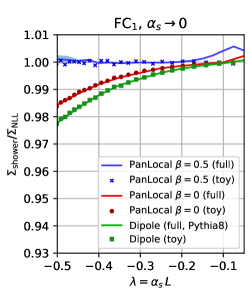
Figure 3: Comparison of the ratio $\Sigma_{\text{shower}}/\Sigma_{\text{NLL}}$ between the toy shower and the full shower for three reference observables ($\sqrt{y_{23}}$, $B_{W}$ and $\text{FC}_{1}$), in the limit $\alpha_{s}\to 0$, as a function of $\alpha_{s}L$. For the full showers the figure shows the ratio of the shower prediction to the full NLL result, while for the toy shower it shows the ratio to the CAESAR-like toy shower. Three full showers are shown in each plot, each compared to the corresponding toy shower. The PanLocal full showers are shown in their dipole variants (identical conclusions hold for the antenna variant). Small $(0.5\%$) issues at $\lambda\gtrsim-0.1$ are a consequence of the fact that for the largest of the $\alpha_{s}$ values used in the extrapolation, the corresponding $L$ values do not quite satisfy $e^{L}\ll 1$.

.2.4 Fixed-order results

In all-order results, whether for the full shower or the toy shower, a key difficulty is to unambiguously sort through different logarithmic orders. The limit $\alpha_{s}\to 0$ that we use is essential in this respect, but the accessible range of $\alpha_{s}$ values remains limited, and a fixed-order expansion provides an alternative way of identifying parametrically dominant logarithmic terms that might come with a small coefficient.

The expansion of the cross section $\Sigma(L)=\sum_{n=0}{\bar{\alpha}}^{n}\Sigma_{n}(L)$ for an observable $V$ to be below some threshold $e^{L}$ can be written as follows

$$\Sigma(L)=\sum_{m,n}\left[\frac{1}{m!}\prod_{i=1}^{m}\left({\bar{\alpha}}\,\int d\Phi_{i}^{\text{real}}\right)\right]\left[\frac{1}{n!}\prod_{i=1}^{n}\left(-{\bar{\alpha}}\,\int d\Phi_{i}^{\text{virt}}\right)\right]\Theta(L-\ln V(\mathcal{I}(p_{1}^{\text{real}},\ldots,p_{m}^{\text{real}})))\,,$$ (31)

where $d\Phi_{i}$ is given by

$$d\Phi_{i}\equiv d\hat{\eta}_{i}\frac{1}{2\pi}\frac{d^{2}\hat{\boldsymbol{p}}_{\perp,i}}{{\hat{p}}_{\perp,i}^{2}}\Theta(-\ln\hat{p}_{\perp,i}>|\hat{\eta}_{i}|)\,.$$ (32)

The insertion operator $\mathcal{I}(p_{1}^{\text{real}},\ldots,p_{m}^{\text{real}})$ in Eq. (31) inserts the emissions in order of decreasing $\ln v=\ln\hat{p}_{\perp,i}-\beta|\hat{\eta}_{i}|$ with the appropriate recoil prescription for the given shower, e.g. Eq. (23) for dipole showers.

A direct evaluation of Eq. (31) leads to terms with up to $2n$ logarithms for the coefficient of ${\bar{\alpha}}^{n}$, from the exponentiation of ${\bar{\alpha}}L^{2}$ structures. For observables that exponentiate, and at fixed coupling, these terms disappear in $\ln\Sigma(L)$, leaving at most terms ${\bar{\alpha}}^{n}L^{m}$ with $m\leq n$. In a numerical (Monte Carlo) calculation of $\ln\Sigma$, one could evaluate individual terms at different orders in the ${\bar{\alpha}}$ expansion of $\Sigma(L)$ and then combine them to obtain the expansion of $\ln\Sigma(L)$. However this would lead to large cancellations between ${\bar{\alpha}}^{n}L^{2n}$ terms coming from Monte Carlo calculations at distinct orders, with uncorrelated statistical errors.

Instead, we take the approach of directly evaluating the expansion of

$$F\equiv\exp(-{\bar{\alpha}}\Sigma_{1}(L))\Sigma(L)\,,$$ (33)

where $\Sigma_{1}(L)$ is the coefficient of ${\bar{\alpha}}$ in the ${\bar{\alpha}}$ series expansion of $\Sigma(L)$. A necessary (but not sufficient) condition for an NLL-correct shower, in the fixed-coupling approximation of our toy model, is that $F$ should only have terms ${\bar{\alpha}}^{n}L^{m}$ with $m\leq n$, like $\ln\Sigma(L)$. Note that with running coupling there would be terms ${\bar{\alpha}}^{n}L^{n+1}$, and it would make more sense to use an analogue of $F$ in which the exponential pre-factor was adjusted for running coupling effects. The non-trivial result starts at second order, and writing $F=\sum_{n}{\bar{\alpha}}^{n}F_{n}$, the first few terms are

$$F_{2}(L)\equiv[\exp(-{\bar{\alpha}}\Sigma_{1}(L))\Sigma(L)]_{2} =\frac{1}{2!}\int d\Phi_{1}d\Phi_{2}\left(\Theta_{12}-\Theta_{1}\Theta_{2}\right),$$ (34a)

$$F_{3}(L)\equiv[\exp(-{\bar{\alpha}}\Sigma_{1}(L))\Sigma(L)]_{3} =\frac{1}{3!}\int d\Phi_{1}d\Phi_{2}d\Phi_{3}\left(\Theta_{123}-\Theta_{12}\Theta_{3}-\Theta_{23}\Theta_{1}-\Theta_{13}\Theta_{2}+2\Theta_{1}\Theta_{2}\Theta_{3}\right),$$ (34b)

$$F_{4}(L)\equiv[\exp(-{\bar{\alpha}}\Sigma_{1}(L))\Sigma(L)]_{4} =\frac{1}{4!}\int d\Phi_{1}d\Phi_{2}d\Phi_{3}d\Phi_{4}(\Theta_{1234}-\Theta_{123}\Theta_{4}-\Theta_{124}\Theta_{3}-\Theta_{134}\Theta_{2}-\Theta_{234}\Theta_{1}$$

$$\qquad\qquad\qquad\qquad\qquad\quad+\Theta_{12}\Theta_{3}\Theta_{4}+\Theta_{13}\Theta_{2}\Theta_{4}+\Theta_{14}\Theta_{2}\Theta_{3}+\Theta_{23}\Theta_{1}\Theta_{4}$$

$$\qquad\qquad\qquad\qquad\qquad\quad+\Theta_{24}\Theta_{1}\Theta_{3}+\Theta_{34}\Theta_{1}\Theta_{2}-3\Theta_{1}\Theta_{2}\Theta_{3}\Theta_{4}),$$ (34c)

where we have introduced the shorthand

$$\Theta_{i\ldots n}\equiv\Theta[L-\ln V(\mathcal{I}(p_{i},\ldots,p_{n}))]\,.$$ (35)

In practice we evaluate the difference between a given shower and the CAESAR result $\delta F_{n}(L)\equiv F_{n}^{\text{shower}}(L)-F_{n}^{\text{CAESAR}}(L)$, so as to remove known NLL terms. In a NLL-correct shower, the $\delta F$ should at most have contributions ${\bar{\alpha}}^{n}L^{m}$ with $m<n$. It will be convenient to study $\delta F_{n}/L^{n}$, which should go to zero for NLL-accurate showers for large negative $L$. If it tends to a non-zero constant, that will signal NLL failure.

Figure 4: Fixed order results from the toy implementation of the standard dipole showers. The plots show the difference between the toy dipole shower and the (NLL-correct) CAESAR results for the $F_{n}$ coefficient of ${\bar{\alpha}}^{n}$ in the expansion of Eq. (33), divided by $L^{n}$. For an NLL-correct shower, the results should tend to zero for large negative $L$. The first row shows the result of $n=3$, the second row that of $n=4$. The columns correspond to different observables (thrust, slice transverse momentum and hemisphere $\sqrt{y_{23}}$). Observe how the results tend to constants (NLL discrepancy) or demonstrate a linear or even quadratic dependence on $L$ (super-leading logarithms). The coefficients have been fitted taking into account correlations between points, and we include powers down to $L^{-3}$ in the fit of $\delta F_{n}/L^{n}$. The fit range is from $-100$ to $-5$ and the quoted error includes both the (statistical) fit uncertainty and the difference in coefficients obtained with the range $[-100,-10]$ (added in quadrature).

A subset of results for dipole showers is shown in Fig. 4. The left-hand column of plots is for the thrust observable and shows $\delta F_{3}(L)/L^{3}$ (top) and $\delta F_{4}(L)/L^{4}$ (bottom) as a function of $L$. At order $\alpha_{s}^{3}$ one sees that the result tends to a constant, signifying an $\alpha_{s}^{3}L^{3}$ term and NLL failure (as reported in the revised version of Ref. Dasgupta et al. (2018)). Rather surprising, however, is that $\delta F_{4}/L^{4}$ (lower-left plot of Fig. 4) appears to have a linear behaviour at large negative $L$, signalling a term $\alpha_{s}^{4}L^{5}$. Such terms are super-leading, in the sense they are larger than any term that should be present in $F(L)$ (or in $\ln\Sigma$) for rIRC safe Banfi et al. (2005) observables in our fixed-coupling approximation. We have found such terms to be present for dipole showers for all global observables with $\beta_{\text{obs}}>0$ and there is strong reason to believe that they are related to sub-leading terms $\alpha_{s}^{2}L$ being enhanced by powers of $\alpha_{s}L^{2}$, giving $\alpha_{s}^{n}L^{2n-3}$. The toy shower cannot accurately predict the coefficients of all such terms in the full shower, because they are affected also by secondary radiation (while the toy model has only primary radiation). However the conclusion that there are such terms is, we believe, robust.

Let us now examine two non-global observables: the transverse momentum in a slice ($S^{\text{slice}}_{\beta=0,\Delta=1}$) and a hemisphere $\sqrt{y_{23}}$ (angular-ordered Durham) jet resolution parameter ($M_{R,\beta=0}$). The toy-shower $F_{n}(L)/L^{n}$ results are shown in the middle and right-hand columns, respectively, of Fig. 4. The slice looks similar to the thrust case, with $\alpha_{s}^{3}L^{3}$ and $\alpha_{s}^{4}L^{5}$ terms. The hemisphere $\sqrt{y_{23}}$ ($M_{R,\beta=0}$) observable has $\alpha_{s}^{3}L^{4}$ and $\alpha_{s}^{4}L^{6}$ terms. The fact that this observable has one additional logarithm makes its analytical calculation somewhat easier (cf. section .3 below). Note that the toy shower is not, in general, suitable for evaluating single-logarithmic ($\alpha_{s}^{n}L^{n}$) terms for non-global observables. However, once again, the existence of such terms in the toy model signals their existence also in the full shower.

It is natural to ask why we do not see the impact of super-leading logarithms in our all-order results. This will be easier to discuss below, once we have explained their origin in detail.

We close this section by illustrating the kind of result that one expects to obtain for a NLL-correct shower. This is shown in Fig. 5 for the PanLocal $\beta=1/2$ shower, again at third and fourth order. In all cases, $\delta F_{n}/L^{n}$ tends to zero for large negative $L$, as required for NLL correctness.

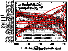
Figure 5: Analogue of Fig. 4, demonstrating the absence of NLL (or super-leading) issues at fixed order in the toy version of the PanLocal $\beta=0.5$ shower. At order ${\bar{\alpha}}^{4}$, we include fit terms down to $L^{-4}$.

.3 Super-leading logarithms

.3.1 Hemisphere max $p_{\perp}$

The simplest observable with which to understand super-leading logarithms is $M_{R,\beta=0}$ (or just $M_{R,0}$ for brevity), the maximum $p_{\perp}$ of emissions in the right hemisphere, because the super-leading terms are visible already from order $\alpha_{s}^{3}$. In the toy-model approach involving only soft primary emissions and fixed-coupling, the correct all-orders result for this observable is $\Sigma=e^{-{\bar{\alpha}}L^{2}/2}$, amounting to exponentiation of the leading-order result. The full QCD NLL result would additionally require inclusion of hard-collinear single-logarithmic corrections, a resummation of non-global logarithms, and running coupling effects. Such contributions are not included in our toy shower and so do not enter into our discussion below.

We are interested here in the fixed-order results for the difference, $\delta F$, between dipole showers and the correct NLL result (i.e. the CAESAR result from section .2). Recall that $F$ was defined in Eq. (33) and that for $n\leq 3$ $\delta F_{n}$ is equivalent to $\delta(\ln\Sigma)_{n}$. A NLL discrepancy between the dipole shower and the correct result would reveal itself via single-logarithmic terms $\alpha_{s}^{n}L^{n}$ in $\delta F$, while for a NLL correct shower $\delta F$ should contain terms that are at most ${\cal O}\!\left(\alpha_{s}^{n}L^{n-1}\right)$.

We start by examining order $\alpha_{s}^{2}$, where $M_{R,0}$ already reveals a NLL discrepancy, due to the recoil issue, i.e. one finds an $\alpha_{s}^{2}L^{2}$ term in the difference between the dipole shower and the correct NLL result. To calculate the coefficient of this $\alpha_{s}^{2}L^{2}$ term we use the method we introduced in Ref. Dasgupta et al. (2018) and examine dipole showers with evolution variable $v=p_{\perp}$. We consider two emissions with values of the shower evolution variable $\hat{p}_{\perp,1}$ and $\hat{p}_{\perp,2}$ respectively, with $\hat{p}_{\perp,1}>\hat{p}_{\perp,2}=\zeta\hat{p}_{\perp,1}$. The NLL order $\alpha_{s}^{2}$ discrepancy arises from a situation where the first emission has $\hat{\eta}_{1}>0$, i.e. is emitted in the right hemisphere $\cal{H}_{R}$, and has its transverse momentum modified by receiving recoil from the second emission also emitted in the right hemisphere. (The contribution from $p_{2}$ in the left-hand hemisphere vanishes after azimuthal integration.) The second emission then must have rapidity $\hat{\eta}_{2}<\frac{1}{2}(\hat{\eta}_{1}-\ln\hat{p}_{\perp 1})$ (cf. Eq. (24)), and the transverse momentum for the first emission is modified so that $\hat{p}_{\perp,1}\to p_{\perp,1}=\hat{p}_{\perp,1}\sqrt{1+\zeta^{2}-2\zeta\cos\phi}$. We then obtain, for the difference between the dipole shower and the correct result,

$${\bar{\alpha}}^{2}\delta F_{2}={\bar{\alpha}}^{2}\int_{0}^{1}\frac{d\hat{p}_{\perp,1}}{\hat{p}_{\perp,1}}\int_{0}^{\ln 1/\hat{p}_{\perp,1}}d\hat{\eta}_{1}\int_{0}^{1}\frac{d\zeta}{\zeta}\int_{0}^{\frac{1}{2}\left(\hat{\eta}_{1}+\ln 1/\hat{p}_{\perp,1}\right)}d\hat{\eta}_{2}\int_{0}^{2\pi}\frac{d\phi}{2\pi}\times\\ \times\left[\Theta\left(v-{\max}(p_{\perp,1},\zeta\hat{p}_{\perp,1}\right))-\Theta\left(v-\hat{p}_{\perp,1}\right)\right],$$ (36)

where $\bar{\alpha}=2C_{F}\alpha_{s}/\pi$ and $v$ is the maximum allowed value of $M_{R,0}$. There are also configurations where $\hat{p}_{1}$ is close to the hemisphere boundary, and gets pulled in/out by an emission $\hat{p}_{2}$ in the unmeasured hemisphere. This could contribute at $\alpha_{s}^{2}L^{2}$, but after azimuthal averaging yields zero. Defining $f_{\text{max}}=\max\left(\zeta,\sqrt{1+\zeta^{2}-2\zeta\cos\phi}\right)$ and $L=\ln v$ and carrying out the required integrals gives the result

$${\bar{\alpha}}^{2}\delta F_{2}=-\frac{3}{4}\bar{\alpha}^{2}L^{2}\int\frac{d\phi}{2\pi}\frac{d\zeta}{\zeta}\ln f_{\text{max}}+\mathcal{O}\left(\bar{\alpha}^{2}L\right)=-0.0685389\,\bar{\alpha}^{2}L^{2}+\mathcal{O}({\bar{\alpha}}^{2}L).$$ (37)

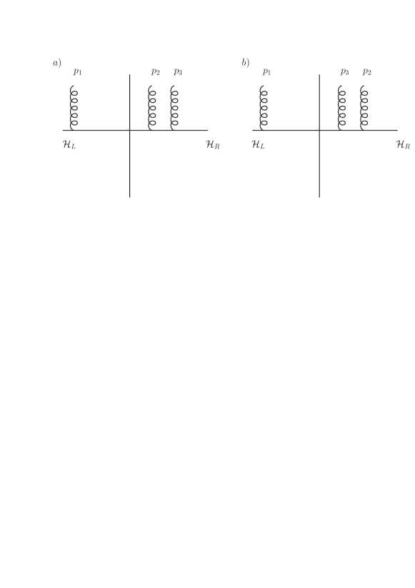
Figure 6: Figure showing emission $p_{1}$ in the left hemisphere and emissions $p_{2}$ and $p_{3}$ in the right hemisphere. On the left we show region a) where $\eta_{3}>\eta_{2}$ while on the right we show region b) where $\eta_{2}>\eta_{3}>0$. In region b) the condition for $p_{3}$ to give recoil to $p_{2}$ depends on $p_{\perp,1}$ and $\eta_{1}$, which gives rise to a mismatch with the case where $p_{1}$ is virtual, resulting in a super-leading logarithm as explained in the text.

Now we turn to order $\alpha_{s}^{3}$. To obtain $\delta\ln\Sigma_{3}$ we need to consider $p_{\perp}$ ordered parton configurations with three real emissions as well as those with two real emissions and a virtual emission. At this order we have

$${\bar{\alpha}}^{3}\delta F_{3}={\bar{\alpha}}^{3}(\delta\Sigma_{3}-\Sigma_{1}\,\delta F_{2})={\bar{\alpha}}^{3}\delta\Sigma_{3}-\frac{3}{8}\bar{\alpha}^{3}L^{4}\int\frac{d\zeta}{\zeta}\frac{d\phi}{2\pi}\ln f_{\mathrm{max}}+\mathcal{O}\left(\bar{\alpha}^{3}L^{3}\right),$$ (38)

where we note the presence of an $\bar{\alpha}^{3}L^{4}$ term which arises from the product of the double-logarithmic leading-order term, ${\bar{\alpha}}\Sigma_{1}=-\frac{1}{2}\bar{\alpha}L^{2}+\mathcal{O}\left(\bar{\alpha}L\right)$, and the recoil discrepancy ${\bar{\alpha}}^{2}\delta\Sigma_{2}$ in Eq. (37). For the discrepancy between dipole showers and the NLL result to be at most single-logarithmic, we should see that this $\bar{\alpha}^{3}L^{4}$ term cancels against a similar term in ${\bar{\alpha}}^{3}\delta\Sigma_{3}$.

In order to obtain the $\bar{\alpha}^{3}L^{4}$ term from ${\bar{\alpha}}^{3}\delta\Sigma_{3}$ we first consider the same two-parton configuration that gives the $\bar{\alpha}^{2}L^{2}$ term for ${\bar{\alpha}}^{2}\delta\Sigma_{2}$, alongside an additional virtual emission. We label the virtual emission $p_{1}$, the two real emissions $p_{2}$ and $p_{3}$ and consider the ordering $\hat{p}_{\perp,1}\gg\hat{p}_{\perp,2}>\hat{p}_{\perp,3}$ so that $p_{2}$ absorbs recoil from the emission of $p_{3}$. Integrating over the full rapidity range $\ln 1/\hat{p}_{\perp,1}>\hat{\eta}_{1}>-\ln 1/\hat{p}_{\perp,1}$ and over $\hat{p}_{\perp,1}$ in the range $1>\hat{p}_{\perp,1}>\hat{p}_{\perp,2}$, produces a factor $-\ln^{2}\hat{p}_{\perp,2}$, with the minus sign accounting for unitarity. It is simple to repeat the calculation that yields $\delta\Sigma_{2}$, using emissions $p_{2}$ and $p_{3}$ and multiplied by this additional factor accounting for the virtual emission, to obtain

$${\bar{\alpha}}^{3}\delta\Sigma^{p_{1}\,\text{virtual}}_{3}=-{\bar{\alpha}}L^{2}\delta\Sigma_{2}=\frac{3}{4}\bar{\alpha}^{3}L^{4}\int\frac{d\phi}{2\pi}\frac{d\zeta}{\zeta}\ln f_{\text{max}}+\mathcal{O}\left(\bar{\alpha}^{3}L^{3}\right).$$ (39)

Next we consider the situation where emission $p_{1}$ is real. To produce the $\bar{\alpha}^{3}L^{4}$ term we require that emission $p_{1}$, which has the largest transverse momentum and is emitted first in the shower, should not affect the observable, which is the case when $p_{1}\in\mathcal{H}_{L}$ i.e. $\hat{\eta}_{1}<0$. We also require that $p_{3}$ gives recoil to $p_{2}$ rather than to $p_{1}$, since we are again examining situations that lead to a difference between dipole showers and the correct result.

There are then two distinct regions to be considered. In region a) we have the situation shown on the left in Fig. 6, where $\hat{\eta}_{3}>\hat{\eta}_{2}$. In this situation $p_{3}$ can only give recoil to $p_{2}$ and one is free to integrate over $\hat{\eta}_{1}$ and $\hat{p}_{\perp,1}$ such that $p_{1}$ is in $\mathcal{H}_{L}$. The integral over $\hat{\eta}$ of all emissions and over $\hat{p}_{\perp,1}$ gives

$$\mathcal{V}_{\text{a}}=\int_{\hat{p}_{\perp,2}}^{1}\frac{d\hat{p}_{\perp,1}}{\hat{p}_{\perp,1}}\int_{-\ln 1/\hat{p}_{\perp,1}}^{0}d\hat{\eta}_{1}\int_{0}^{\ln 1/\hat{p}_{\perp,2}}d\hat{\eta}_{2}\int_{\hat{\eta}_{2}}^{\frac{1}{2}\left(\hat{\eta}_{2}+\ln 1/\hat{p}_{\perp,2}\right)}d\hat{\eta}_{3}=\frac{1}{8}\ln^{4}\hat{p}_{\perp,2}.$$ (40)

On the other hand for region b) shown on the right of Fig. 6, the condition that $p_{2}$ receives recoil from $p_{3}$ is affected by the presence of $p_{1}$. In this region the rapidity constraints are more involved and the integral over $\hat{\eta}_{1},\hat{p}_{\perp,1}$ cannot be performed independently as was the case in region a) and also for the virtual correction. The integral over $\hat{\eta}$ of all emissions and over $\hat{p}_{\perp,1}$ now gives

$$\mathcal{V}_{\text{b}}=\int_{\hat{p}_{\perp,2}}^{1}\frac{d\hat{p}_{\perp,1}}{\hat{p}_{\perp,1}}\int_{-\ln 1/\hat{p}_{\perp,1}}^{0}d\hat{\eta}_{1}\int_{0}^{\ln 1/\hat{p}_{\perp,2}}d\hat{\eta}_{2}\int_{0}^{\hat{\eta}_{2}}d\hat{\eta}_{3}\,\Theta\left(\hat{\eta}_{3}-\frac{1}{2}\left(\hat{\eta}_{1}+\hat{\eta}_{2}+\ln\frac{\hat{p}_{\perp,2}}{\hat{p}_{\perp,1}}\right)\right)=\frac{11}{48}\ln^{4}\hat{p}_{\perp,2}.$$ (41)

Combining the contributions from Eqs. (40) and (41) we can perform the remaining integrals over $\hat{p}_{\perp,2}$, $\zeta$ and $\phi$ to obtain

$${\bar{\alpha}}^{3}\delta\Sigma_{3}^{\text{all real}}=\frac{17}{48}\int\frac{d\phi}{2\pi}\frac{d\zeta}{\zeta}\int_{0}^{1}\frac{d\hat{p}_{\perp,2}}{\hat{p}_{\perp,2}}\ln^{4}{\hat{p}_{\perp,2}}\left[\Theta\left(v-\hat{p}_{\perp,2}f_{\mathrm{max}}\right)-\Theta\left(v-\hat{p}_{\perp,2}\right)\right]=-\frac{17}{48}\bar{\alpha}^{3}L^{4}\int\frac{d\phi}{2\pi}\frac{d\zeta}{\zeta}\ln f_{\text{max}}+\mathcal{O}\left(\bar{\alpha}^{3}L^{3}\right).$$ (42)

Adding together real and virtual contributions, neglecting any $\mathcal{O}\left(\bar{\alpha}^{3}L^{3}\right)$ terms, we then have $\delta\Sigma_{3}=\delta\Sigma_{3}^{\text{all real}}+\delta\Sigma^{p_{1}\,\text{virtual}}_{3}$ and using Eq. (38) we are left with a surviving super-leading logarithmic contribution:

$${\bar{\alpha}}^{3}\delta F_{3}=\frac{1}{48}\bar{\alpha}^{3}L^{4}\int\frac{d\phi}{2\pi}\frac{d\zeta}{\zeta}\ln f_{\text{max}}=0.00190386\,\bar{\alpha}^{3}L^{4}+{\cal O}\!\left({\bar{\alpha}}^{3}L^{3}\right),$$ (43)

in agreement with the fit in Fig. 4, to within errors. At next order in $\alpha_{s}$, one needs to consider up to two emissions in the unobserved hemisphere, each of which brings a factor $\alpha_{s}L^{2}$, leading to the $\alpha_{s}^{4}L^{6}$ term seen in Fig. 4.

.3.2 Considerations at all orders

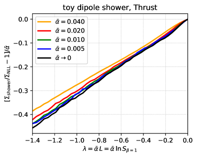
Figure 7: Toy-shower all-order result for the thrust ($S_{\beta=1}$, Eq. (25)). Left: $\Sigma_{\text{dipole}}/\Sigma_{\text{NLL}}$, where the NLL result is given by running the CAESAR version of the shower. Four values of ${\bar{\alpha}}$ are shown, together with the extrapolation to ${\bar{\alpha}}=0$, showing that the all-order dipole-shower result (in our usual limit of fixed ${\bar{\alpha}}L$ and ${\bar{\alpha}}\to 0$) is consistent with the NLL result, despite the super-leading logarithmic terms that are visible in Fig. 4. Right: $(\Sigma_{\text{dipole}}/\Sigma_{\text{NLL}}-1)/{\bar{\alpha}}$, again for three values of ${\bar{\alpha}}$ and the extrapolation to ${\bar{\alpha}}=0$. The fact that these curves converge is a sign that the all-order (toy) dipole-shower discrepancy with respect to NLL behaves as a term that vanishes proportionally to ${\bar{\alpha}}$, i.e. as an NNLL term. The results here involve fixed coupling, i.e. they do not include a correction of the form of Eq. (30).

It is perhaps surprising that observables with super-leading logarithms in the toy shower should resum to give apparent good agreement with NLL in the full shower (cf. amber triangles in Fig. 2 right). Fig. 7 shows the toy-shower all-order result for one of these observables, the thrust, so that we can compare fixed-order and all-order results within a single framework (using the same underlying shower insertion code, as described in section .2). The left-hand plot shows the usual $\Sigma_{\text{dipole}}/\Sigma_{\text{NLL}}$ ratio as a function of ${\bar{\alpha}}L$ for several ${\bar{\alpha}}$ values, together with its extrapolation to ${\bar{\alpha}}=0$. The extrapolation is consistent with unity, i.e. apparent all-order agreement with the NLL result, as in the full shower. Note that for ${\bar{\alpha}}L=-1.5$, the ${\bar{\alpha}}^{3}L^{3}$ and ${\bar{\alpha}}^{4}L^{5}$ terms from Fig. 4 would respectively contribute $-0.054$ and $-0.87$ to the ${\bar{\alpha}}=0.01$ ($L=-150$) line in Fig. 7 (left). The all-order results undoubtedly have the statistical power to resolve such effects, yet do not show any sign of them.

The right-hand plot of the same figure shows $(\Sigma_{\text{dipole}}/\Sigma_{\text{NLL}}-1)/{\bar{\alpha}}$ and its extrapolation to ${\bar{\alpha}}=0$. This serves as a verification that in this specific limit (i.e. ${\bar{\alpha}}L$ fixed and ${\bar{\alpha}}\to 0$, implying ${\bar{\alpha}}L^{2}\to\infty$) any all-order discrepancies with respect to the NLL result mimic a standard NNLL, or even higher order, correction.

The presence of super-leading logarithms that evade detection at all orders is a particularly unpleasant characteristic of dipole showers, because it risks giving a false sense of security as to the validity of the underlying logarithmic structure. An analytic study of the all-order resummation of the super-leading logarithms is beyond the scope of this manuscript. However, a reader wishing to understand how an apparently large effect at fixed order seemingly vanishes at all orders, could consider the following argument. For all the amber triangles in Fig. 2, one contribution to the super-leading logarithms comes from an ${\bar{\alpha}}^{2}L$ (NNLL) contribution promoted by additional factors of ${\bar{\alpha}}L^{2}$. The ${\bar{\alpha}}^{2}L$ term arises when a first emission $a$, contributing a factor ${\bar{\alpha}}$, absorbs recoil from a second, unresolved, emission $b$ with commensurate $p_{\perp}$. Integrating over the rapidity of the second emission yields a factor ${\bar{\alpha}}L$, giving the overall ${\bar{\alpha}}^{2}L$. The ${\bar{\alpha}}L^{2}$ enhancement factor that arises at next order comes about because there is a double logarithmic region for an emission $c$ with $\hat{p}_{\perp,c}\gg\hat{p}_{\perp,a}$ that alters whether $b$ can induce recoil for $a$ (for example if $\hat{\eta}_{c}<\hat{\eta}_{b}$, then one has a dipole chain $(a-c-b)$ and $a$ will not receive recoil from $b$). At all orders, the typical rapidity extent ($|\hat{\eta}_{a}-\hat{\eta}_{b}|$) in which one can have an $a-b$ dipole without any other higher-$p_{\perp}$ particles in between can become of order either $1/\sqrt{{\bar{\alpha}}}$ or $1$, depending on the context. This causes the original ${\bar{\alpha}}^{2}L$ factor to have $L$ replaced at all orders by $1/\sqrt{{\bar{\alpha}}}$ or $1$ respectively, giving ${\bar{\alpha}}^{3/2}$ or ${\bar{\alpha}}^{2}$, i.e. even smaller than NNLL (which itself can arise from a multitude of sources).

.4 Lund-plane declustering for $e^{+}e^{-}$ collisions and $\Delta\psi$ resummation

In this section we introduce the definition of the azimuthal separation between two Lund-plane declusterings Dreyer et al. (2018) in $e^{+}e^{-}\to\text{ jets}$ events. This observable has been used in the letter to test the azimuthal dependence of the effective double-soft strongly angular-ordered squared amplitude in different showers. A proper definition of the azimuthal angle $\psi$ of a declustering $p_{i}\to p_{j}+p_{k}$ requires the introduction of a dynamic reference axis such that $\psi$ is always defined with respect to the direction of $p_{i}$. We introduce the reference axes $\vec{n}_{x}=(1,0,0)$, $\vec{n}_{y}=(0,1,0)$, and $\vec{n}_{z}=(0,0,1)$. We denote a generic rotation matrix $R$, which rotates the $z$ axis to a direction $\vec{d}$ that has an inclination $\theta$ and an azimuth $\phi$,

$$R(\vec{d}\,)\equiv R(\theta,\phi)=\left(\begin{array}[]{ccc}\cos(\phi)&-\sin(\phi)&0\\ \sin(\phi)&\cos(\phi)&0\\ 0&0&1\end{array}\right)\left(\begin{array}[]{ccc}\cos(\theta)&0&\sin(\theta)\\ 0&1&0\\ -\sin(\theta)&0&\cos(\theta)\\ \end{array}\right)\left(\begin{array}[]{ccc}\cos(\phi)&+\sin(\phi)&0\\ -\sin(\phi)&\cos(\phi)&0\\ 0&0&1\end{array}\right)\,.$$ (44)

We start with a configuration with two hard jets $j_{1}$ and $j_{2}$ in the event, and we set the initial reference direction as $\vec{d}_{\text{ev}}\propto\vec{j}_{1}-\vec{j}_{2}$, with $j_{1}$ being the jet with the larger (positive) value of $p_{z}$, and we normalise $|\vec{d}_{\text{ev}}|=1$. We define the initial rotation matrix $\mathcal{R}_{0}=R(\vec{d}_{\text{ev}})$, and we assign a sign $s=1$ to the direction of the jet $j_{1}$ (with the larger $z$ component), and a sign $s=-1$ to the direction of $j_{2}$.

Consider a declustering $p_{i}\to p_{j}+p_{k}$, primary or secondary, which we label as being step $n$ in the declustering sequence constructed with the Cambridge algorithm Dokshitzer et al. (1997) (four momenta are combined according to the standard $E$ scheme, i.e. a $4$-vector sum Cacciari et al. (2012)). We introduce the reference directions of the declustering,

$$\vec{u}_{i}=\frac{\vec{p}_{i}}{|\vec{p}_{i}|}\,,\qquad\delta\vec{u}_{kj}=\vec{u}_{k}-\vec{u}_{j}.$$ (45)

We then determine an updated rotation matrix as

$$\mathcal{R}_{n}=R(\mathcal{R}_{n-1}^{-1}(su_{i}))\cdot\mathcal{R}_{n-1},$$ (46)

where $\mathcal{R}_{n-1}$ is the rotation matrix relative to the previous declustering stage. We finally evaluate $\psi$ for this declustering as

$$\psi=\text{atan2}(\delta\vec{u}_{kj}.\mathcal{R}_{n}.\vec{n}_{y},\,\delta\vec{u}_{kj}.\mathcal{R}_{n}.\vec{n}_{x})\,.$$ (47)

The Lund-plane declustering technology allows the inspection of the structure of the primary and secondary radiation in the event. We consider the two highest-$p_{\perp}$ primary Lund declusterings as an IRC safe proxy for the two leading (i.e. highest-$p_{\perp}$) primary emissions, which are the main element of NLL resummations for global observables. The azimuthal separation $|\Delta\psi_{12}|$ used in Fig. 1 is simply defined as the absolute value of the difference between the $\psi$ angles of the two leading declusterings.

Specifically, we show the $|\Delta\psi_{12}|$ distribution for a given bin of the leading declustering ($k_{t1}$), with an additional constraint on the next highest $p_{\perp}$ primary declustering ($k_{t2}$) of the form

$$k_{t,12}^{\rm min}<\frac{k_{t2}}{k_{t1}}<k_{t,12}^{\rm max};\quad k_{t,12}^{\rm min}=0.3\,,\quad k_{t,12}^{\rm max}=0.5\,.$$ (48)

We consider the distribution normalised to the NLL vetoed cross section $\Sigma(k_{t1})$ given in refs. Banfi et al. (2002). The NLL prediction for this observable reads

$$\Sigma(\Delta\psi_{12},k_{t2}|k_{t1})\equiv\frac{\Sigma(k_{t1},k_{t2},|\Delta\psi_{12}|)}{\Sigma(k_{t1})}=\frac{1}{\pi}\left(e^{R^{\prime}(\lambda)\ln k_{t,12}^{\rm max}}-e^{R^{\prime}(\lambda)\ln k_{t,12}^{\rm min}}\right)\,,\qquad R^{\prime}(\lambda)\equiv\frac{4C_{F}}{\pi}\frac{\lambda}{1-2\beta_{0}\lambda}\,,$$ (49)

where $\lambda=\alpha_{s}\ln(Q/k_{t1})$, and $\beta_{0}=(11C_{A}-2n_{F})/(12\pi)$.

.5 Subjet multiplicities

The scaling of particle multiplicities with centre-of-mass energy is one of the few observables that has long been included among the logarithmic structure tests routinely carried out for parton showers Marchesini and Webber (1984). Relative to the infrared collinear-safe global (shape-like) observables and the non-global slice observable that we have concentrated on for NLL accuracy tests here, it has the interesting feature of being sensitive to the full nested soft-collinear multiple branching structure. Multiplicity itself is not infrared and collinear safe, however subjet multiplicities for specific jet algorithms are. We therefore concentrate on the latter. They are known to NLL accuracy Catani et al. (1992b) for the $e^{+}e^{-}$ Durham ($k_{t}$) jet algorithm Catani et al. (1991b). Whereas for global shape-like observables NLL implies control of terms $\alpha_{s}^{n}L^{n}$ in $\ln\Sigma$, NLL for multiplicities implies control of terms $\alpha_{s}^{n}L^{2n-1}$ in the multiplicity itself. Accordingly we take the limit $\alpha_{s}\to 0$ for fixed $\alpha_{s}L^{2}$ (rather than fixed $\alpha_{s}L$). Therefore, for an N^pLL result, we should control terms suppressed by $\alpha_{s}^{p/2}$ relative to the LL result. With $L=\frac{1}{2}\ln y_{\text{cut}}$, we consider

$$\frac{N^{\text{subjet}}_{\text{shower}}(\alpha_{s},\alpha_{s}L^{2})/N^{\text{subjet}}_{\text{NLL}}(\alpha_{s},\alpha_{s}L^{2})-1}{\sqrt{\alpha_{s}}}\,$$ (50)

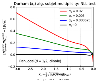
Figure 8: Checks of the $k_{t}$ algorithm subjet multiplicity. Left: the multiplicity as a function of $\frac{1}{2}\sqrt{\alpha_{s}(Q)}\ln y_{cut}$, comparing the PanLocal $\beta=0.5$ shower (dipole variant) with the NLL prediction, for two choices of $\alpha_{s}$. Right: Eq. (50) for the same shower, for several $\alpha_{s}$ values, together with the $\alpha_{s}\to 0$ limit.

and in particular take its $\alpha_{s}\to 0$ limit while keeping $\alpha_{s}L^{2}$ fixed. Eq. (50) should vanish as $\sqrt{\alpha_{s}}$ if the shower is NLL accurate. Fig. 8 (left) illustrates the multiplicity as a function of $\frac{1}{2}\sqrt{\alpha_{s}(Q)}\ln y_{cut}$ for two values of $\alpha_{s}$, comparing the PanLocal $\beta=0.5$ shower (in its dipole variant) to the NLL result. The right-hand plot shows Eq. (50) for the same shower, for three values of $\alpha_{s}$ as well as the extrapolation to $\alpha_{s}=0$. It illustrates the good agreement across the range of $\frac{1}{2}\sqrt{\alpha_{s}(Q)}\ln y_{cut}$ values (with the usual exception of the region close to $0$, which is not sufficiently asymptotic). Other showers give similar results. Note that the $\alpha_{s}\to 0$ extrapolation is more delicate for the multiplicity than for other observables, because of the effective expansion in powers of $\sqrt{\alpha_{s}}$ rather than $\alpha_{s}$. This implies a need for a broader range of $\alpha_{s}$ values in order to obtain reliable results.

.6 Considerations for $\alpha_{s}\to 0$ limits of showers

To reach a conclusion about NLL correctness of showers, it has been crucial for us to be able to disentangle NLL terms from NNLL and yet higher-order contributions. This was achieved by considering the $\alpha_{s}\to 0$ limit of

$$\frac{\Sigma_{\text{shower}}^{\text{obs}}(\alpha_{s},\alpha_{s}L)}{\Sigma_{\text{NLL}}^{\text{obs}}(\alpha_{s},\alpha_{s}L)}\,,$$ (51)

for each given observable at fixed $\alpha_{s}L$. The requirement of small $\alpha_{s}$ implies large $L$. Other than for the subjet multiplicity studies discussed in the previous section, the smallest $\alpha_{s}$ values used in producing Fig. 2 were either $0.005$ or $0.01$, depending on the specific observable and shower.

Consider for now the smallest value, $\alpha_{s}=0.005$. To achieve $\alpha_{s}L=-0.5$, one needs $L=-100$. In practice we typically add an event generation buffer of $B=18$ units of the logarithm below the value of interest for the observable. The limit on the precision on the observable distribution is then expected to be proportional to $e^{-B}$. The logarithm of the span of scales in the event generation, roughly $-118$, takes us into a regime that is far beyond that needed for parton showers in normal phenomenological contexts and introduces a number of challenges. In what follows, we outline some of those challenges and the main solutions we have adopted.

.6.1 The challenges

Particle multiplicities. The logarithm of the particle multiplicity $N$ in an event scales as $\sqrt{\alpha_{s}L^{2}}$. As we take $\alpha_{s}\to 0$ with $\alpha_{s}L$ fixed, $\alpha_{s}L^{2}=(\alpha_{s}L)^{2}/\alpha_{s}$ grows large and particle multiplicities become huge. With $\alpha_{s}=0.005$ and generation down to $\ln k_{t}/Q=-118$, the average multiplicity, $\langle N\rangle$, is of the order of $10^{5}$. For computational strategies in event generation and subsequent analysis that scale as $N$ this is at the edge of accessibility. Where they scale as $N^{2}$ (or worse) it can well be beyond it.

Numerical precision. Covering a range of momenta that stretches from $1$ (in units of the centre-of-mass energy $Q$) down to $e^{-118}\simeq 6\cdot 10^{-52}$ poses challenges. This is particularly the case for the calculation of the dot products that arise, for example, in Eqs. (2),(3). Normal double-precision evaluations can fail already when $k_{t}/Q\sim\sqrt{\epsilon}$, where $\epsilon\sim 10^{-16}$ is machine precision.

Size of cross sections. The cross section $\Sigma(L)$ for (say) the $\sqrt{y_{23}}$ observable to be below $e^{L}$ scales as $\Sigma(L)\simeq\exp[-2C_{F}\alpha_{s}L^{2}/\pi]$ at fixed coupling. Including full LL and NLL terms with running coupling, for $\alpha_{s}=0.005$ and $\alpha_{s}L=-0.5$ one obtains $\Sigma(L)\sim 10^{-29}$. If one uses unweighted events, then a precision determination of $\Sigma(L)$ requires that one needs to generate substantially more than $1/\Sigma(L)$ events. This is simply not feasible.

.6.2 Solutions adopted

We have taken a hybrid approach to these challenges. Firstly, insofar as possible, we have attempted to limit the challenge. For example we use techniques similar to those of Ref. Kleiss and Verheyen (2016) supplemented with a Roulette Wheel Lipowski and Lipowska (2011) choice of dipole to eliminate the $N^{2}$ scaling for all showers except the PanGlobal one. (We believe $N^{2}$ scaling for the PanGlobal showers could perhaps also be eliminated with suitable caching, but so far this wasn’t a critical necessity).

To address the precision issue, in the small-angle limit we use cross-products rather than dot products, which generically remain viable down to angles of $\epsilon$ rather than $\sqrt{\epsilon}$. A further improvement is to align the initial $q\bar{q}$ event along the $z$ axis. Then there is almost no limit on the smallest angle that can be calculated with respect to the original $q\bar{q}$ direction, and when the shower produces an emitter at an angle $\theta$ with respect to the $z$ axis, the smallest angle that can subsequently be calculated with respect to that emitter is $\epsilon\theta$. When these techniques reach their limit, we switch to the use of dd_real and qd_real types Hida et al. (2000), though thanks to other advances below, this was necessary mainly for code testing and for the runs used to determine average multiplicities. One could also envisage techniques to handle arbitrarily small angles fully in double precision.

A second element of our approach is to avoid generating emissions in regions that are of no relevance to a given study. We make an estimate for each emission of the most it could contribute to that observable ($L_{\text{approx}}=\ln k_{t}-\beta_{\text{obs}}|\eta|$ with $\eta=\bar{\eta}+\frac{1}{\beta}\ln\rho$ for the PanScales showers, ignoring distinctions between primary and secondary emissions) and then avoid generating emissions whose contributions would be below $e^{-B}$ times the largest contribution so far in the shower. This dynamic cutoff reduces multiplicities to a manageable level and also keeps us in a regime where we can carry out calculations in double precision rather than dd_real and qd_real.

One potential concern about the dynamic cutoff is that while it is safe from the point of view of the global observables (because they are rIRC safe), it does cut out phase-space regions associated with the generation of super-leading logarithms in dipole showers. However the fact that our full-shower results (with the dynamic cutoff) agree with the toy-shower results (which use the full primary phase space, i.e. no dynamic cutoff) gives us some reassurance that the dynamic cutoff is not generating misleading all-order conclusions in Fig. 2. Ultimately part of the reason that there is no issue here is that the super-leading logarithms are anyway strongly reduced by all-order resummation effects. This parametrically suppresses their effect in the $\alpha_{s}\to 0$ limit and restricts the relevant phase-space region to a band of width $1/\sqrt{\alpha_{s}}$ below the observable boundary, a width that we account for by the generation buffer $B$.

The final element that we bring to the problem is weighted event generation. When $\beta_{\text{PS}}=\beta_{\text{obs}}$, this is fairly straightforward (to avoid ambiguity in this paragraph, we add a “PS” subscript to the $\beta$ used in the parton shower ordering variable). We split event generation into bins of the first-emission $\ln v$. For a given bin we include an event weight proportional to the Sudakov above the upper edge of the $\ln v$ bin. When $\beta_{\text{PS}}=\beta_{\text{obs}}$ there is a strong correlation between the shower variable $\ln v$ for the first emission and the value of the observable and so the weight distribution for a given observable bin is relatively compact. This approach works less well when $\beta_{\text{PS}}\neq\beta_{\text{obs}}$ and in some challenging cases (notably $\beta_{\text{PS}}=\frac{1}{2}$, $\beta_{\text{obs}}=0$) further refinements are needed. There, we choose a bin for the highest $L_{\text{approx}}$ that we will accept, start the shower with the least negative $\ln v$ that can be in that bin (with an appropriate Sudakov weight) and then immediately reject an event if at any stage in its showering one produces an emission with an $L_{\text{approx}}$ that is larger than the upper edge of the bin. This rejection tends to happen in the early stages of the generation, so there is a limited cost to generating the (many) events that ultimately get rejected. It is conceivable that there might be more sophisticated approaches, but this one was sufficient in order to reach the few-per-mil precisions needed on the $\alpha_{s}\to 0$ extrapolations at fixed $\alpha_{s}L$ for Fig. 2, though it only just allowed us to explore the region down to $\alpha_{s}L=-0.5$ for $\beta_{\text{PS}}=0.5$ showers.

Note that extrapolations to $\alpha_{s}=0$ are performed using a polynomial of degree $n-1$ for $n$ values of $\alpha_{s}$.

References

- Buckley et al. (2011) A. Buckley et al., Phys. Rept. 504, 145 (2011), arXiv:1101.2599 [hep-ph] .
- Sjostrand and Skands (2005) T. Sjostrand and P. Z. Skands, Eur. Phys. J. C39, 129 (2005), arXiv:hep-ph/0408302 [hep-ph] .
- Giele et al. (2008) W. T. Giele, D. A. Kosower, and P. Z. Skands, Phys. Rev. D78, 014026 (2008), arXiv:0707.3652 [hep-ph] .
- Nagy and Soper (2007) Z. Nagy and D. E. Soper, JHEP 09, 114 (2007), arXiv:0706.0017 [hep-ph] .
- Schumann and Krauss (2008) S. Schumann and F. Krauss, JHEP 03, 038 (2008), arXiv:0709.1027 [hep-ph] .
- Platzer and Gieseke (2011) S. Platzer and S. Gieseke, JHEP 01, 024 (2011), arXiv:0909.5593 [hep-ph] .
- Jadach et al. (2010) S. Jadach, A. Kusina, M. Skrzypek, and M. Slawinska, Proceedings, 10th DESY Workshop on Elementary Particle Theory: Loops and Legs in Quantum Field Theory: Woerlitz, Germany, April 25-30, 2010, Nucl. Phys. Proc. Suppl. 205-206, 295 (2010), arXiv:1007.2437 [hep-ph] .
- Nagy and Soper (2012) Z. Nagy and D. E. Soper, JHEP 06, 044 (2012), arXiv:1202.4496 [hep-ph] .
- Nagy and Soper (2014) Z. Nagy and D. E. Soper, JHEP 06, 097 (2014), arXiv:1401.6364 [hep-ph] .
- Nagy and Soper (2015) Z. Nagy and D. E. Soper, JHEP 07, 119 (2015), arXiv:1501.00778 [hep-ph] .
- Hoeche and Prestel (2015) S. Hoeche and S. Prestel, Eur. Phys. J. C75, 461 (2015), arXiv:1506.05057 [hep-ph] .
- Li and Skands (2017) H. T. Li and P. Skands, Phys. Lett. B771, 59 (2017), arXiv:1611.00013 [hep-ph] .
- Jadach et al. (2016) S. Jadach, A. Kusina, W. Placzek, and M. Skrzypek, JHEP 08, 092 (2016), arXiv:1606.01238 [hep-ph] .
- Fischer et al. (2016) N. Fischer, S. Prestel, M. Ritzmann, and P. Skands, Eur. Phys. J. C76, 589 (2016), arXiv:1605.06142 [hep-ph] .
- Nagy and Soper (2016) Z. Nagy and D. E. Soper, JHEP 10, 019 (2016), arXiv:1605.05845 [hep-ph] .
- Fischer et al. (2017) N. Fischer, A. Lifson, and P. Skands, Eur. Phys. J. C77, 719 (2017), arXiv:1708.01736 [hep-ph] .
- Hoeche et al. (2017) S. Hoeche, F. Krauss, and S. Prestel, JHEP 10, 093 (2017), arXiv:1705.00982 [hep-ph] .
- Hoeche and Prestel (2017) S. Hoeche and S. Prestel, Phys. Rev. D96, 074017 (2017), arXiv:1705.00742 [hep-ph] .
- Nagy and Soper (2018) Z. Nagy and D. E. Soper, Phys. Rev. D98, 014034 (2018), arXiv:1705.08093 [hep-ph] .
- Cabouat and Sjöstrand (2018) B. Cabouat and T. Sjöstrand, Eur. Phys. J. C78, 226 (2018), arXiv:1710.00391 [hep-ph] .
- Dulat et al. (2018) F. Dulat, S. Hoeche, and S. Prestel, Phys. Rev. D98, 074013 (2018), arXiv:1805.03757 [hep-ph] .
- Plaetzer et al. (2018) S. Plaetzer, M. Sjodahl, and J. Thorén, JHEP 11, 009 (2018), arXiv:1808.00332 [hep-ph] .
- Ángeles Martínez et al. (2018) R. Ángeles Martínez, M. De Angelis, J. R. Forshaw, S. Plaetzer, and M. H. Seymour, JHEP 05, 044 (2018), arXiv:1802.08531 [hep-ph] .
- Isaacson and Prestel (2019) J. Isaacson and S. Prestel, Phys. Rev. D99, 014021 (2019), arXiv:1806.10102 [hep-ph] .
- Brooks and Skands (2019) H. Brooks and P. Skands, Phys.Rev.D 100, 076006 (2019), arXiv:1907.08980 [hep-ph] .
- Forshaw et al. (2019) J. R. Forshaw, J. Holguin, and S. Plaetzer, (2019), 10.1007/JHEP08(2019)145, [JHEP08,145(2019)], arXiv:1905.08686 [hep-ph] .
- Nagy and Soper (2019) Z. Nagy and D. E. Soper, Phys. Rev. D100, 074005 (2019), arXiv:1908.11420 [hep-ph] .
- Hoeche and Reichelt (2020) S. Hoeche and D. Reichelt, (2020), arXiv:2001.11492 [hep-ph] .
- Buckley et al. (2010) A. Buckley, H. Hoeth, H. Lacker, H. Schulz, and J. E. von Seggern, Eur. Phys. J. C65, 331 (2010), arXiv:0907.2973 [hep-ph] .
- Skands (2010) P. Z. Skands, Phys. Rev. D82, 074018 (2010), arXiv:1005.3457 [hep-ph] .
- Keith Ellis and Zanderighi (2019) R. Keith Ellis and G. Zanderighi, in From My Vast Repertoire …: Guido Altarelli’s Legacy, edited by A. Levy, S. Forte, and G. Ridolfi (World Scientific, Singapore, 2019) pp. 31–52.
- Azzi et al. (2019) P. Azzi et al., CERN Yellow Rep. Monogr. 7, 1 (2019), arXiv:1902.04070 [hep-ph] .
- Cepeda et al. (2019) M. Cepeda et al., CERN Yellow Rep. Monogr. 7, 221 (2019), arXiv:1902.00134 [hep-ph] .
- Cid Vidal et al. (2019) X. Cid Vidal et al., CERN Yellow Rep. Monogr. 7, 585 (2019), arXiv:1812.07831 [hep-ph] .
- Marchesini and Webber (1984) G. Marchesini and B. R. Webber, Nucl. Phys. B238, 1 (1984).
- Banfi et al. (2007) A. Banfi, G. Corcella, and M. Dasgupta, JHEP 03, 050 (2007), arXiv:hep-ph/0612282 [hep-ph] .
- Dasgupta et al. (2018) M. Dasgupta, F. A. Dreyer, K. Hamilton, P. F. Monni, and G. P. Salam, JHEP 09, 033 (2018), arXiv:1805.09327 [hep-ph] .
- Bewick et al. (2019) G. Bewick, S. Ferrario Ravasio, P. Richardson, and M. H. Seymour, (2019), arXiv:1904.11866 [hep-ph] .
- Marchesini and Webber (1988) G. Marchesini and B. R. Webber, Nucl. Phys. B310, 461 (1988).
- Corcella et al. (2001) G. Corcella, I. G. Knowles, G. Marchesini, S. Moretti, K. Odagiri, P. Richardson, M. H. Seymour, and B. R. Webber, JHEP 01, 010 (2001), arXiv:hep-ph/0011363 [hep-ph] .
- Bahr et al. (2008) M. Bahr et al., Eur. Phys. J. C58, 639 (2008), arXiv:0803.0883 [hep-ph] .
- Gustafson and Pettersson (1988) G. Gustafson and U. Pettersson, Nucl. Phys. B306, 746 (1988).
- Lonnblad (1992) L. Lonnblad, Comput. Phys. Commun. 71, 15 (1992).
- Webber (1986) B. R. Webber, Ann. Rev. Nucl. Part. Sci. 36, 253 (1986).
- Collins (1988) J. C. Collins, Nucl. Phys. B304, 794 (1988).
- Catani and Grazzini (2011) S. Catani and M. Grazzini, Nucl. Phys. B845, 297 (2011), arXiv:1011.3918 [hep-ph] .
- Banfi et al. (2005) A. Banfi, G. P. Salam, and G. Zanderighi, JHEP 03, 073 (2005), arXiv:hep-ph/0407286 [hep-ph] .
- Knowles (1990) I. G. Knowles, Comput. Phys. Commun. 58, 271 (1990).
- Nagy and Soper (2008) Z. Nagy and D. E. Soper, JHEP 07, 025 (2008), arXiv:0805.0216 [hep-ph] .
- Richardson and Webster (2020) P. Richardson and S. Webster, Eur. Phys. J. C80, 83 (2020), arXiv:1807.01955 [hep-ph] .
- Dasgupta et al. (2020) M. Dasgupta, F. A. Dreyer, K. Hamilton, P. F. Monni, G. P. Salam, and G. Soyez, Supplemental material to this letter (2020).
- Andersson et al. (1989) B. Andersson, G. Gustafson, L. Lonnblad, and U. Pettersson, Z. Phys. C43, 625 (1989).
- Banfi et al. (2002) A. Banfi, G. P. Salam, and G. Zanderighi, JHEP 01, 018 (2002), arXiv:hep-ph/0112156 [hep-ph] .
- Gribov and Lipatov (1972) V. N. Gribov and L. N. Lipatov, Sov. J. Nucl. Phys. 15, 438 (1972), [Yad. Fiz.15,781(1972)].
- Altarelli and Parisi (1977) G. Altarelli and G. Parisi, Nucl. Phys. B126, 298 (1977).
- Dokshitzer (1977) Y. L. Dokshitzer, Sov. Phys. JETP 46, 641 (1977), [Zh. Eksp. Teor. Fiz.73,1216(1977)].
- Behring et al. (2019) A. Behring, K. Melnikov, R. Rietkerk, L. Tancredi, and C. Wever, Phys.Rev.D 100, 114034 (2019), arXiv:1910.10059 [hep-ph] .
- Catani et al. (1991a) S. Catani, B. R. Webber, and G. Marchesini, Nucl. Phys. B349, 635 (1991a).
- Abada et al. (2019) A. Abada et al. (FCC), Eur. Phys. J. ST 228, 755 (2019).
- Hoeche et al. (2018) S. Hoeche, D. Reichelt, and F. Siegert, JHEP 01, 118 (2018), arXiv:1711.03497 [hep-ph] .
- Hida et al. (2000) Y. Hida, X. S. Li, and D. H. Bailey, in 15th IEEE Symposium on Computer Arithmetic (2000) pp. 155–162.
- Lipowski and Lipowska (2011) A. Lipowski and D. Lipowska, CoRR abs/1109.3627 (2011), arXiv:1109.3627 .
- Kleiss and Verheyen (2016) R. Kleiss and R. Verheyen, Eur. Phys. J. C76, 359 (2016), arXiv:1605.09246 [hep-ph] .
- Dreyer et al. (2018) F. A. Dreyer, G. P. Salam, and G. Soyez, JHEP 12, 064 (2018), arXiv:1807.04758 [hep-ph] .
- Andrews et al. (2018) H. A. Andrews et al., (2018), arXiv:1808.03689 [hep-ph] .
- Cacciari et al. (2012) M. Cacciari, G. P. Salam, and G. Soyez, Eur. Phys. J. C72, 1896 (2012), arXiv:1111.6097 [hep-ph] .
- Larkoski et al. (2020) A. J. Larkoski, I. Moult, and B. Nachman, Phys. Rept. 841, 1 (2020), arXiv:1709.04464 [hep-ph] .
- Dokshitzer et al. (1997) Y. L. Dokshitzer, G. D. Leder, S. Moretti, and B. R. Webber, JHEP 08, 001 (1997), arXiv:hep-ph/9707323 [hep-ph] .
- Catani et al. (1992a) S. Catani, G. Turnock, and B. R. Webber, Phys. Lett. B295, 269 (1992a).
- Brandt et al. (1964) S. Brandt, C. Peyrou, R. Sosnowski, and A. Wroblewski, Phys. Lett. 12, 57 (1964).
- Farhi (1977) E. Farhi, Phys. Rev. Lett. 39, 1587 (1977).
- Dasgupta and Salam (2002) M. Dasgupta and G. P. Salam, JHEP 03, 017 (2002), arXiv:hep-ph/0203009 [hep-ph] .
- Dokshitzer et al. (1998) Y. L. Dokshitzer, A. Lucenti, G. Marchesini, and G. P. Salam, JHEP 01, 011 (1998), arXiv:hep-ph/9801324 [hep-ph] .
- Catani et al. (1993) S. Catani, L. Trentadue, G. Turnock, and B. R. Webber, Nucl. Phys. B407, 3 (1993).
- Catani et al. (1991b) S. Catani, Y. L. Dokshitzer, M. Olsson, G. Turnock, and B. R. Webber, Phys. Lett. B269, 432 (1991b).
- Catani et al. (1992b) S. Catani, Y. L. Dokshitzer, F. Fiorani, and B. R. Webber, Nucl. Phys. B377, 445 (1992b).
- Brown and Stirling (1990) N. Brown and W. J. Stirling, Phys. Lett. B252, 657 (1990).
- Forshaw et al. (2006) J. R. Forshaw, A. Kyrieleis, and M. H. Seymour, JHEP 08, 059 (2006), arXiv:hep-ph/0604094 [hep-ph] .
- Catani et al. (2012) S. Catani, D. de Florian, and G. Rodrigo, JHEP 07, 026 (2012), arXiv:1112.4405 [hep-ph] .